testing of peak demand- limiting using … of peak demand-limiting using thermal mass at a small...
TRANSCRIPT
TESTING OF PEAK DEMAND-LIMITING USING THERMAL MASS AT A SMALL COMMERCIAL BUILDING
Submitted to the: Demand Response Research Center
Prepared by Kyoung-Ho Lee and James E. Braun Purdue University
Steve Fredrickson Southern California Edison
Kyle Konis and Edward Arens University of California at Berkeley
July 2007
ACKNOWLEDGEMENTS This work was coordinated by the Demand Response Research Center and funded by
the California Energy Commission, Public Interest Energy Research Program.
EXECUTIVE SUMMARY This report presents results from field testing and comfort surveys designed to
evaluate peak demand-limiting strategies that utilize both precooling and adjustments of
zone cooling setpoints. The testing was performed over a two-week period at a small
bank building in Palm Desert, California. During the first week test, three kinds of
control strategies were considered:
1) conventional night setup control as a baseline case,
2) a simple linear-rise demand-limiting strategy that involved precooling during the
morning and linear setpoint adjustments during an afternoon demand-limiting
period, and
3) a simple step-up demand-limiting strategy that included precooling in the
morning and resetting of setpoint during the demand-limiting period.
During the second week of testing, a demand-limiting strategy was tested for four days
with setpoint trajectories determined using a weighted-averaging method developed at
Purdue University. Precooling of the building was performed at 70ºF setpoint from 6am
to 12pm and setpoints during the on-peak period from 12pm to 6pm were modulated
from 70 to 78ºF following a trajectory that attempted to minimize peak cooling load.
(The measured temperature at the polling station was a minimum of 1.5 degrees F above
the thermostat setpoint (see figures 24 to 29 in appendix). The baseline was conventional
night-setup control with a 72ºF cooling setpoint temperature during the occupied period.
The demand-limiting tests resulted in greater than 30% reduction of peak air conditioner
power on average for the four tested days which accounted for 0.76W/ft2 peak savings.
The comfort survey revealed that the response of occupants was highly variable at
any given indoor temperature. Statistical analysis of all the data collected, including
baseline days and test days, indicated a significant probability that a given occupant will
vote that the temperature is ‘cool’ at the low setpoint temperature of 70 degrees (between
30 and 50 percent), and ‘warm’ at the upper setpoint of 78 degrees (between 37 and 52
percent) (figure 21). However, only half of these votes are at the level where the
ii
respondent says it ‘bothers’ them. The probability of a given occupant being bothered by
the ‘cool’ temperature at the low setpoint is estimated to be 17 percent and the
probability of a given occupant being bothered by the ‘warm’ temperature at at the upper
setpoint is estimated to be 23 percent. (figure 22). If we assume the neutral temperature
to be between 74 and 75 degrees F, the probability of dissatisfaction (both ‘Too warm! It
bothers me’ and ‘Too cool! It bothers me’) is estimated to be 20 percent.

iii
TABLE OF CONTENTS
ACKNOWLEDGEMENTS................................................................................................. i
EXECUTIVE SUMMARY ................................................................................................. i
INTRODUCTION .............................................................................................................. 4
Background..................................................................................................................... 4
Objectives ....................................................................................................................... 4
Accomplishments............................................................................................................ 4
DESCRIPTION OF TEST FACILITY AND PROCEDURES .......................................... 5
Test Building................................................................................................................... 5
Air Conditioning Equipment .......................................................................................... 8
Data Measurement .......................................................................................................... 8
Setpoint Schedule ........................................................................................................... 9
TEST AND SURVEY RESULTS .................................................................................... 15
Peak Demand Reduction............................................................................................... 15
Comfort Survey Results................................................................................................ 21
Results........................................................................................................................... 21
Visual Analysis of the data ........................................................................................... 22
Logit Regression of Comfort Data................................................................................ 26
CONCLUSIONS............................................................................................................... 30
ACRONYMS.................................................................................................................... 32
REFERENCES ................................................................................................................. 32
Appendix........................................................................................................................... 33
4
INTRODUCTION
Background There have been a few simulated and experimental studies that have demonstrated
potential for reducing peak cooling demand using building thermal mass through control
of zone temperatures for small commercial buildings. Lee and Braun (2006a) developed
a model-based demand-limiting method that relies on a detailed inverse model. The
method was trained using data from the Energy Resource Station building that houses the
Iowa Energy Center and validated experimentally by Lee and Braun (2006b). The test
results showed 30% reductions in peak cooling loads with setpoint adjustments from 70
to 76°F for a 5-hour demand-limiting. These results are consistent with simulation results
that were determined for this facility. Lee and Braun (2006c,d) also developed a more
simplified method, which is termed the weighted-averaging method (WA method) for
determining demand-limiting setpoint trajectories using short-term measurements. The
method doesn’t require a building model and weather data but only requires cooling load
or associated power data. The method was evaluated for different buildings using trained
inverse building models and simulations. Simulation results showed that the method is
effective for peak load reduction compared to optimal control assuming perfect
knowledge of building thermal response and perfect prediction of weather conditions.
Objectives The goal of the current project was to perform field testing to demonstrate peak
cooling demand reduction for a small commercial building using a demand-limiting
control strategy based on the weighted-averaging method of Lee and Braun (2006c) and
to evaluate comfort of occupants. The demand-limiting control strategy in this study
involves precooling a building in the morning at a lower bound of comfort, i.e. 70ºF and
then warming up the building by modulating the cooling setpoint temperatures up to an
upper bound of comfort temperature, i.e. 78ºF.
Accomplishments The resulting demand-limiting strategy was tested for four days in October with clear
sky conditions and a maximum outdoor temperature between 80 and 85ºF. The baseline
was conventional night-setup control with a 72ºF cooling setpoint temperature during the
5
occupied period from 6am to 7pm. The demand-limiting control was performed with
precooling at 70ºF from 6am to 12pm and setpoint adjustment up to 78ºF during an on-
peak period from 12pm to 6pm. The demand-limiting setpoint trajectory was determined
with the WA method developed by Lee and Braun (2006c). The test results showed a
peak air conditioning power reduction of more than 30% or 0.76W/ft2. The comfort
survey showed that the range of precooling and setpoint setups in this test did not affect
the customers significantly, regardless of indoor-outdoor temperature differences. The
bank employees are more likely to be the limiting factor, since their exposure is far
longer. Setpoint limits for employees under precooling conditions have been studied in a
large commercial building located in Visalia (Xu, Brown 2007).
DESCRIPTION OF TEST FACILITY AND PROCEDURES
Test Building The selection criteria for the small commercial building site included:
• a building representative of common construction design of buildings of this
size
• wire-to-wire compatible retrofit for new page-able thermostats
• a building occupancy typical of small commercial facilities in this size range
• located in a hot climate
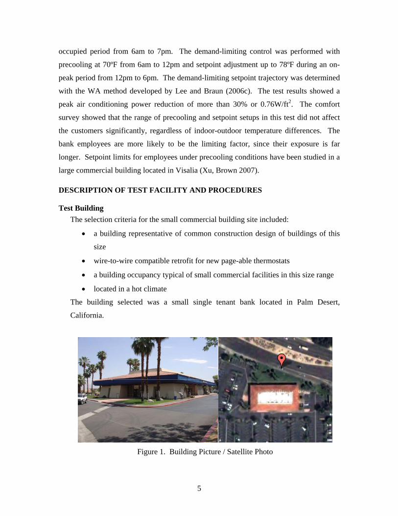
The building selected was a small single tenant bank located in Palm Desert,
California.
Figure 1. Building Picture / Satellite Photo
6
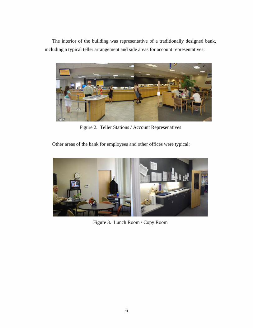
The interior of the building was representative of a traditionally designed bank,
including a typical teller arrangement and side areas for account representatives:
Figure 2. Teller Stations / Account Represenatives
Other areas of the bank for employees and other offices were typical:
Figure 3. Lunch Room / Copy Room
7
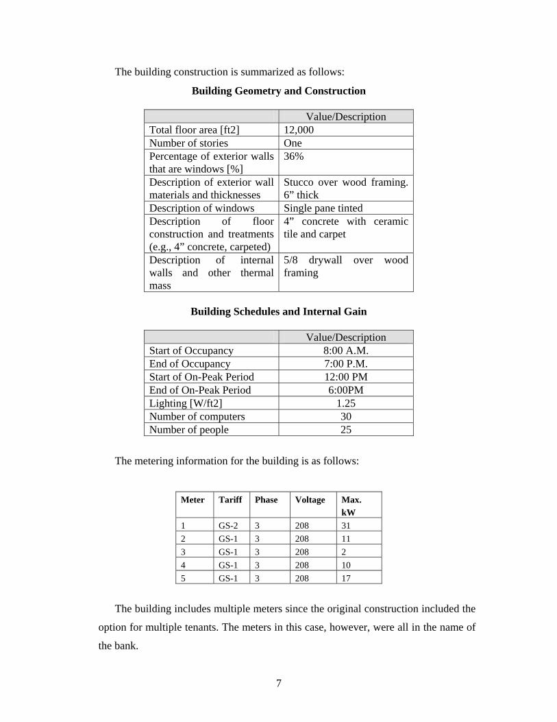
The building construction is summarized as follows:
Building Geometry and Construction
Value/Description Total floor area [ft2] 12,000 Number of stories One Percentage of exterior walls that are windows [%]
36%
Description of exterior wall materials and thicknesses
Stucco over wood framing. 6” thick
Description of windows Single pane tinted Description of floor construction and treatments (e.g., 4” concrete, carpeted)
4” concrete with ceramic tile and carpet
Description of internal walls and other thermal mass
5/8 drywall over wood framing
Building Schedules and Internal Gain
Value/Description
Start of Occupancy 8:00 A.M. End of Occupancy 7:00 P.M. Start of On-Peak Period 12:00 PM End of On-Peak Period 6:00PM Lighting [W/ft2] 1.25 Number of computers 30 Number of people 25
The metering information for the building is as follows:
Meter Tariff Phase Voltage Max. kW
1 GS-2 3 208 31 2 GS-1 3 208 11 3 GS-1 3 208 2 4 GS-1 3 208 10 5 GS-1 3 208 17
The building includes multiple meters since the original construction included the
option for multiple tenants. The meters in this case, however, were all in the name of
the bank.
8
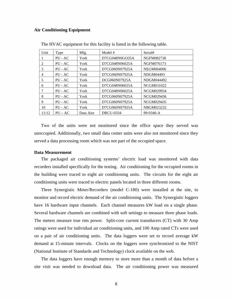
Air Conditioning Equipment
The HVAC equipment for this facility is listed in the following table.
Unit Type Mfg. Model # Serial# 1 PU - AC York D7CG048N0GO35A NGFM082738 2 PU - AC York D7CG048N06025A NGFM076173 3 PU - AC York D7CG060N07925A NEGM064006 4 PU - AC York D7CG060N07925A NDGM04493 5 PU - AC York DCG060N07925A NDGM044492 6 PU - AC York D7CG048N06025A NCGM031022 7 PU - AC York D7CG048N06025A NCGM029934 8 PU - AC York D7CG060N07925A NCGM029436 9 PU - AC York D7CG060N07925A NCGM029435 10 PU - AC York D7CG060N07925A NBGM023232 11/12 PU – AC Data Aire DRCU-0334 99-0346-A
Two of the units were not monitored since the office space they served was
unoccupied. Additionally, two small data center units were also not monitored since they
served a data processing room which was not part of the occupied space.
Data Measurement The packaged air conditioning systems’ electric load was monitored with data
recorders installed specifically for the testing. Air conditioning for the occupied rooms in
the building were traced to eight air conditioning units. The circuits for the eight air
conditioning units were traced to electric panels located in three different rooms.
Three Synergistic Meter/Recorders (model C-180) were installed at the site, to
monitor and record electric demand of the air conditioning units. The Synergistic loggers
have 16 hardware input channels. Each channel measures kW load on a single phase.
Several hardware channels are combined with soft settings to measure three phase loads.
The meters measure true rms power. Split-core current transducers (CT) with 30 Amp
ratings were used for individual air conditioning units, and 100 Amp rated CTs were used
on a pair of air conditioning units. The data loggers were set to record average kW
demand at 15-minute intervals. Clocks on the loggers were synchronized to the NIST
(National Institute of Standards and Technology) clock available on the web.
The data loggers have enough memory to store more than a month of data before a
site visit was needed to download data. The air conditioning power was measured
9
separately using hand-held instruments, to validate the logger data. Total air
conditioning power was determined during post processing as the sum of the individual
recorded data channels.
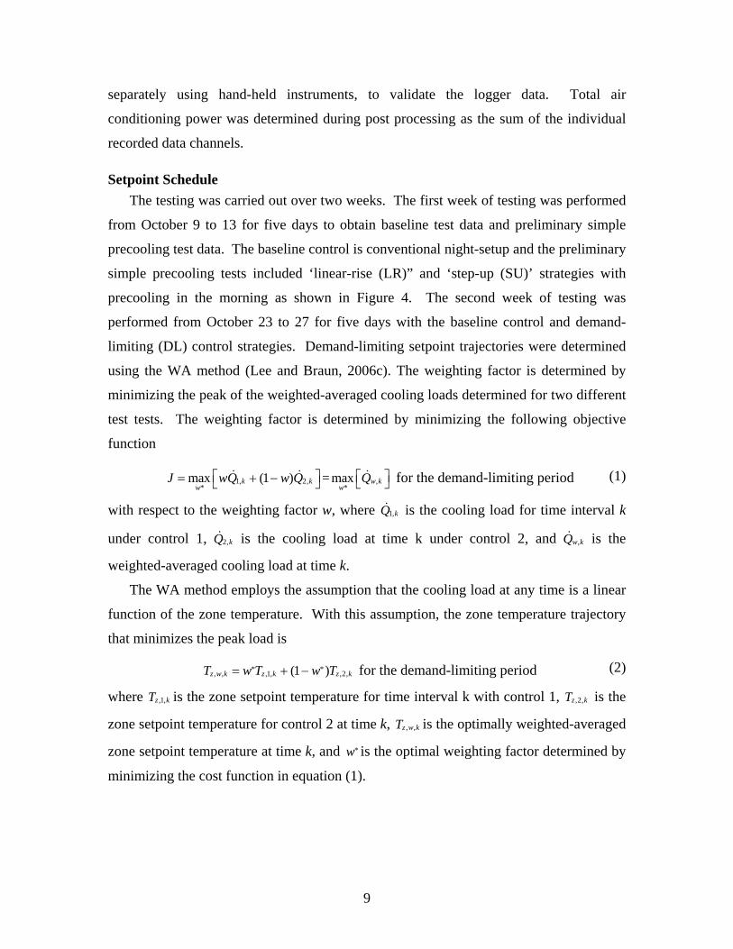
Setpoint Schedule The testing was carried out over two weeks. The first week of testing was performed
from October 9 to 13 for five days to obtain baseline test data and preliminary simple
precooling test data. The baseline control is conventional night-setup and the preliminary
simple precooling tests included ‘linear-rise (LR)” and ‘step-up (SU)’ strategies with
precooling in the morning as shown in Figure 4. The second week of testing was
performed from October 23 to 27 for five days with the baseline control and demand-
limiting (DL) control strategies. Demand-limiting setpoint trajectories were determined
using the WA method (Lee and Braun, 2006c). The weighting factor is determined by
minimizing the peak of the weighted-averaged cooling loads determined for two different
test tests. The weighting factor is determined by minimizing the following objective
function
1, 2, ,* *
max (1 ) = maxk k w kw w
J wQ w Q Q⎡ ⎤ ⎡ ⎤= + −⎣ ⎦ ⎣ ⎦& & & for the demand-limiting period (1)
with respect to the weighting factor w, where 1,kQ& is the cooling load for time interval k
under control 1, 2,kQ& is the cooling load at time k under control 2, and ,w kQ& is the
weighted-averaged cooling load at time k.
The WA method employs the assumption that the cooling load at any time is a linear
function of the zone temperature. With this assumption, the zone temperature trajectory
that minimizes the peak load is
* *, , ,1, ,2,(1 )z w k z k z kT w T w T= + − for the demand-limiting period (2)
where ,1,z kT is the zone setpoint temperature for time interval k with control 1, ,2,z kT is the
zone setpoint temperature for control 2 at time k, , ,z w kT is the optimally weighted-averaged
zone setpoint temperature at time k, and *w is the optimal weighting factor determined by
minimizing the cost function in equation (1).
10
The setpoint trajectory of equation (2) that is obtained from the weighted-averaging is
then adjusted using the following equation (Lee and Braun, 2006c).
, , , , ,z dl k z w k adj kT T T= + Δ (3)
, ,, ,max
, ,maxw k w avg
adj k adjw k w avg
Q QT TQ Q−
Δ =−
& &
& & (4)
where ,w kQ& is the weighted-averaged cooling load using 1,kQ& and 2,kQ& at time k, ,maxadjT is
the maximum allowable adjustment temperature for a given hour (1.0°F in this testing),
and ,w avgQ& is the average of the weighted-averaged cooling load ,w kQ& over the demand-
limiting period which is assumed to be the target peak cooling load.
On-peak
Occupied period
Set
poin
t te
mpe
ratu
re
Time
85oF
6am 12pm 6pm 7pm
72oF
On-peak
Occupied period
Set
poin
t te
mpe
ratu
re
Time
85oF
6am 12pm 6pm 7pm
72oF
(a)
Precooling On-peak
Occupied period
Setp
oint
te
mpe
ratu
re
Time
Step-up
Linear-rise70oF
78oF
85oF
6am 12pm 6pm 7pm
Demand-limiting
Precooling On-peak
Occupied period
Setp
oint
te
mpe
ratu
re
Time
Step-up
Linear-rise70oF
78oF
85oF
6am 12pm 6pm 7pm
Demand-limiting
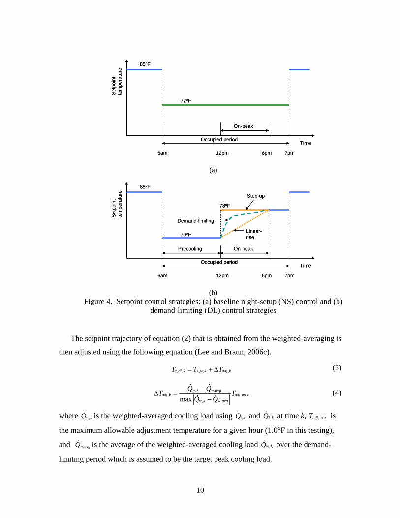
(b) Figure 4. Setpoint control strategies: (a) baseline night-setup (NS) control and (b)
demand-limiting (DL) control strategies
11
The occupied cooling period was from 6am in the morning to 7pm in the evening.
The on-peak period or demand-limiting period was from 12 pm to 6pm for the tests. For
the unoccupied period from 7pm to 6am, the setpoint temperature was setup at 85ºF for
all control strategies.
For the other periods except the two week test period during the summer, the night-
setup control was employed for building cooling.
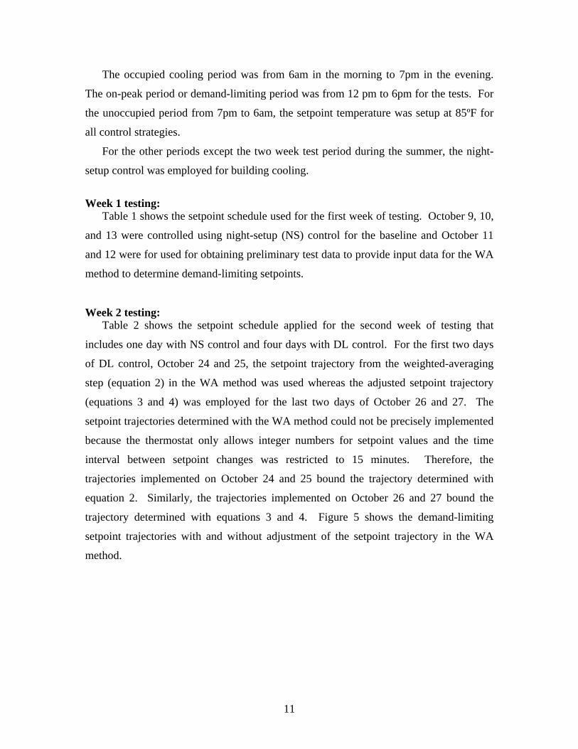
Week 1 testing:
Table 1 shows the setpoint schedule used for the first week of testing. October 9, 10,
and 13 were controlled using night-setup (NS) control for the baseline and October 11
and 12 were for used for obtaining preliminary test data to provide input data for the WA
method to determine demand-limiting setpoints.
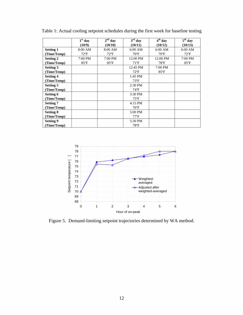
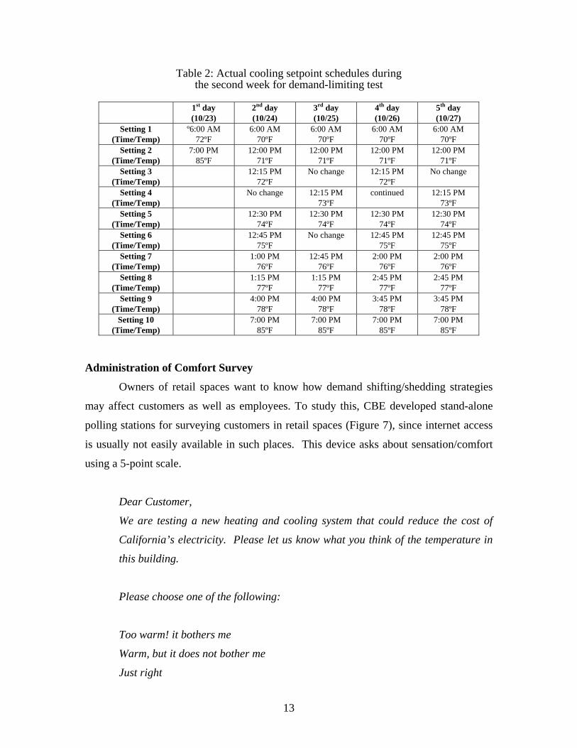
Week 2 testing: Table 2 shows the setpoint schedule applied for the second week of testing that
includes one day with NS control and four days with DL control. For the first two days
of DL control, October 24 and 25, the setpoint trajectory from the weighted-averaging
step (equation 2) in the WA method was used whereas the adjusted setpoint trajectory
(equations 3 and 4) was employed for the last two days of October 26 and 27. The
setpoint trajectories determined with the WA method could not be precisely implemented
because the thermostat only allows integer numbers for setpoint values and the time
interval between setpoint changes was restricted to 15 minutes. Therefore, the
trajectories implemented on October 24 and 25 bound the trajectory determined with
equation 2. Similarly, the trajectories implemented on October 26 and 27 bound the
trajectory determined with equations 3 and 4. Figure 5 shows the demand-limiting
setpoint trajectories with and without adjustment of the setpoint trajectory in the WA
method.
12
Table 1: Actual cooling setpoint schedules during the first week for baseline testing
1st day (10/9)
2nd day (10/10)
3rd day (10/11)
4th day (10/12)
5th day (10/13)
Setting 1 (Time/Temp)
8:00 AM 72ºF
8:00 AM 72ºF
6:00 AM 70ºF
6:00 AM 70ºF
6:00 AM 72ºF
Setting 2 (Time/Temp)
7:00 PM 85ºF
7:00 PM 85ºF
12:00 PM 71ºF
12:00 PM 78ºF
7:00 PM 85ºF
Setting 3 (Time/Temp)
12:45 PM 72ºF
7:00 PM 85ºF
Setting 4 (Time/Temp)
1:45 PM 73ºF
Setting 5 (Time/Temp)
2:30 PM 74ºF
Setting 6 (Time/Temp)
3:30 PM 75ºF
Setting 7 (Time/Temp)
4:15 PM 76ºF
Setting 8 (Time/Temp)
5:00 PM 77ºF
Setting 9 (Time/Temp)
5:30 PM 78ºF
686970717273747576777879
0 1 2 3 4 5 6
Hour of on-peak
Set
poin
t tem
pera
ture
[ �]
Weighted-averagedAdjusted afterweighted-averaged
Figure 5. Demand-limiting setpoint trajectories determined by WA method.
13
Table 2: Actual cooling setpoint schedules during the second week for demand-limiting test
1st day
(10/23) 2nd day (10/24)
3rd day (10/25)
4th day (10/26)
5th day (10/27)
Setting 1 (Time/Temp)
º6:00 AM 72ºF
6:00 AM 70ºF
6:00 AM 70ºF
6:00 AM 70ºF
6:00 AM 70ºF
Setting 2 (Time/Temp)
7:00 PM 85ºF
12:00 PM 71ºF
12:00 PM 71ºF
12:00 PM 71ºF
12:00 PM 71ºF
Setting 3 (Time/Temp)
12:15 PM 72ºF
No change
12:15 PM 72ºF
No change
Setting 4 (Time/Temp)
No change
12:15 PM 73ºF
continued
12:15 PM 73ºF
Setting 5 (Time/Temp)
12:30 PM 74ºF
12:30 PM 74ºF
12:30 PM 74ºF
12:30 PM 74ºF
Setting 6 (Time/Temp)
12:45 PM 75ºF
No change 12:45 PM 75ºF
12:45 PM 75ºF
Setting 7 (Time/Temp)
1:00 PM 76ºF
12:45 PM 76ºF
2:00 PM 76ºF
2:00 PM 76ºF
Setting 8 (Time/Temp)
1:15 PM 77ºF
1:15 PM 77ºF
2:45 PM 77ºF
2:45 PM 77ºF
Setting 9 (Time/Temp)
4:00 PM 78ºF
4:00 PM 78ºF
3:45 PM 78ºF
3:45 PM 78ºF
Setting 10 (Time/Temp)
7:00 PM 85ºF
7:00 PM 85ºF
7:00 PM 85ºF
7:00 PM 85ºF
Administration of Comfort Survey
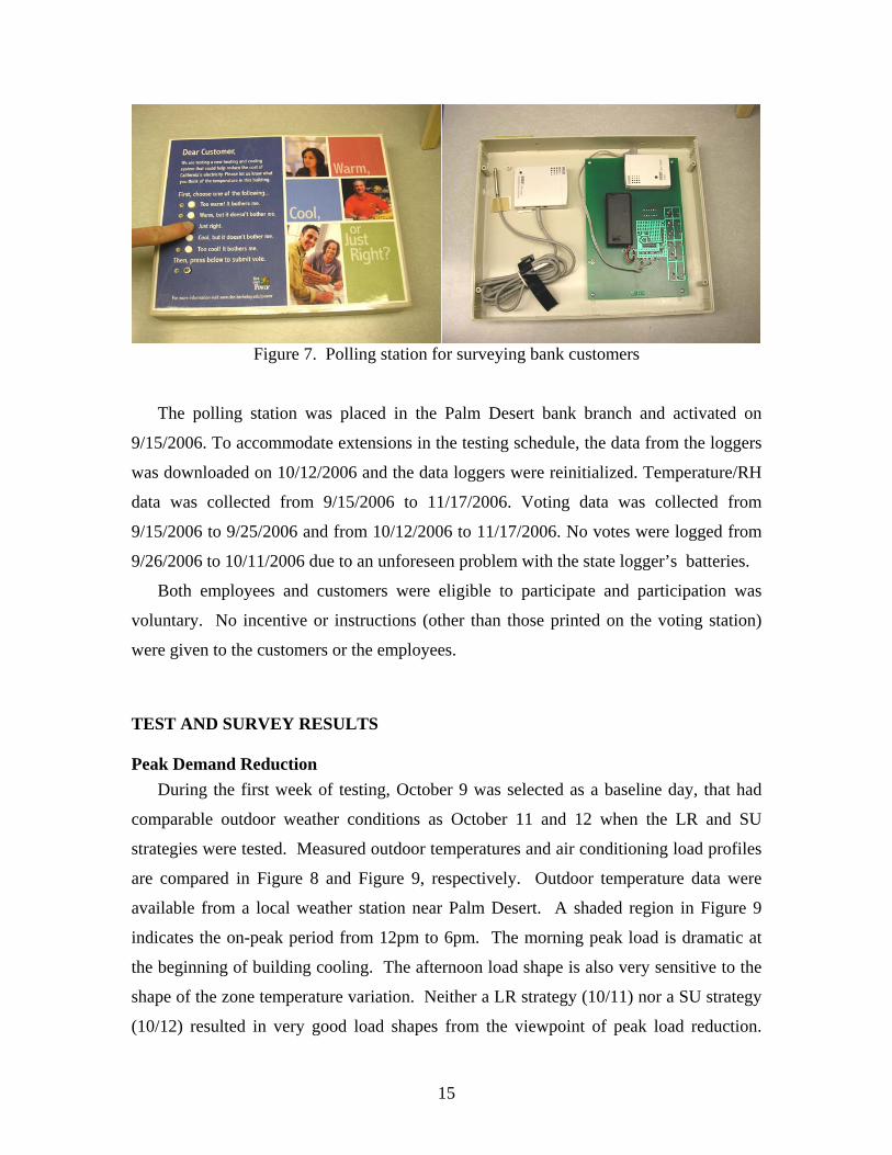
Owners of retail spaces want to know how demand shifting/shedding strategies
may affect customers as well as employees. To study this, CBE developed stand-alone
polling stations for surveying customers in retail spaces (Figure 7), since internet access
is usually not easily available in such places. This device asks about sensation/comfort
using a 5-point scale.
Dear Customer,
We are testing a new heating and cooling system that could reduce the cost of
California’s electricity. Please let us know what you think of the temperature in
this building.
Please choose one of the following:
Too warm! it bothers me
Warm, but it does not bother me
Just right
14
Cool, but it does not bother me
Too Cool! it bothers me
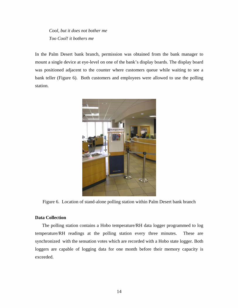
In the Palm Desert bank branch, permission was obtained from the bank manager to
mount a single device at eye-level on one of the bank’s display boards. The display board
was positioned adjacent to the counter where customers queue while waiting to see a
bank teller (Figure 6). Both customers and employees were allowed to use the polling
station.
Figure 6. Location of stand-alone polling station within Palm Desert bank branch
Data Collection
The polling station contains a Hobo temperature/RH data logger programmed to log
temperature/RH readings at the polling station every three minutes. These are
synchronized with the sensation votes which are recorded with a Hobo state logger. Both
loggers are capable of logging data for one month before their memory capacity is
exceeded.
15
Figure 7. Polling station for surveying bank customers
The polling station was placed in the Palm Desert bank branch and activated on
9/15/2006. To accommodate extensions in the testing schedule, the data from the loggers
was downloaded on 10/12/2006 and the data loggers were reinitialized. Temperature/RH
data was collected from 9/15/2006 to 11/17/2006. Voting data was collected from
9/15/2006 to 9/25/2006 and from 10/12/2006 to 11/17/2006. No votes were logged from
9/26/2006 to 10/11/2006 due to an unforeseen problem with the state logger’s batteries.
Both employees and customers were eligible to participate and participation was
voluntary. No incentive or instructions (other than those printed on the voting station)
were given to the customers or the employees.
TEST AND SURVEY RESULTS
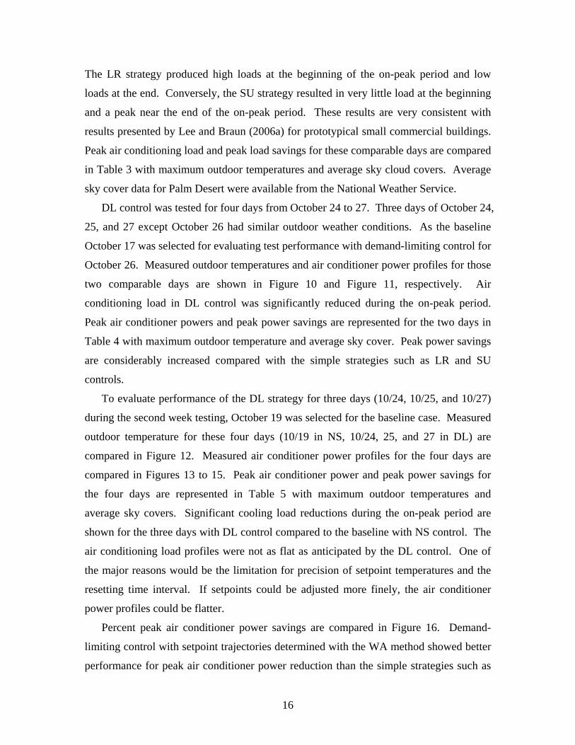
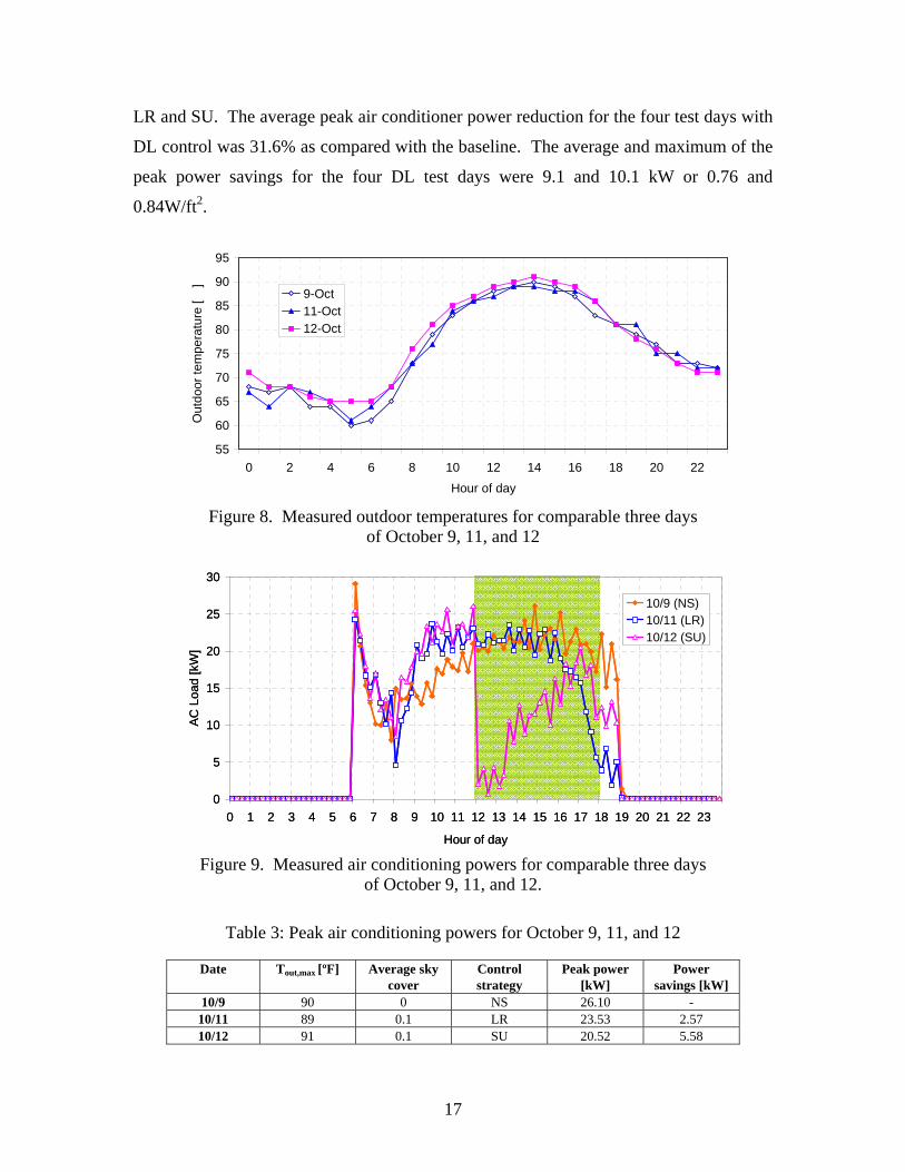
Peak Demand Reduction During the first week of testing, October 9 was selected as a baseline day, that had
comparable outdoor weather conditions as October 11 and 12 when the LR and SU
strategies were tested. Measured outdoor temperatures and air conditioning load profiles
are compared in Figure 8 and Figure 9, respectively. Outdoor temperature data were
available from a local weather station near Palm Desert. A shaded region in Figure 9
indicates the on-peak period from 12pm to 6pm. The morning peak load is dramatic at
the beginning of building cooling. The afternoon load shape is also very sensitive to the
shape of the zone temperature variation. Neither a LR strategy (10/11) nor a SU strategy
(10/12) resulted in very good load shapes from the viewpoint of peak load reduction.
16
The LR strategy produced high loads at the beginning of the on-peak period and low
loads at the end. Conversely, the SU strategy resulted in very little load at the beginning
and a peak near the end of the on-peak period. These results are very consistent with
results presented by Lee and Braun (2006a) for prototypical small commercial buildings.
Peak air conditioning load and peak load savings for these comparable days are compared
in Table 3 with maximum outdoor temperatures and average sky cloud covers. Average
sky cover data for Palm Desert were available from the National Weather Service.
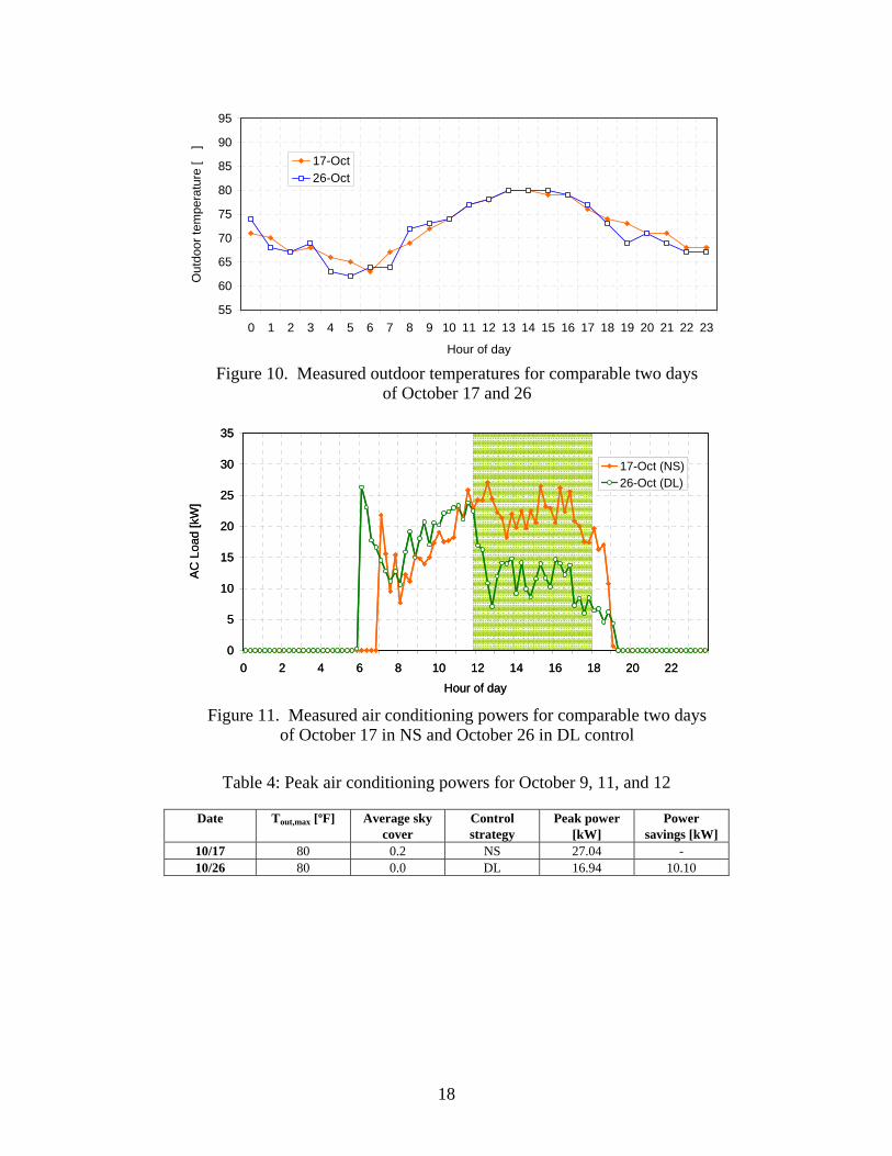
DL control was tested for four days from October 24 to 27. Three days of October 24,
25, and 27 except October 26 had similar outdoor weather conditions. As the baseline
October 17 was selected for evaluating test performance with demand-limiting control for
October 26. Measured outdoor temperatures and air conditioner power profiles for those
two comparable days are shown in Figure 10 and Figure 11, respectively. Air
conditioning load in DL control was significantly reduced during the on-peak period.
Peak air conditioner powers and peak power savings are represented for the two days in
Table 4 with maximum outdoor temperature and average sky cover. Peak power savings
are considerably increased compared with the simple strategies such as LR and SU
controls.
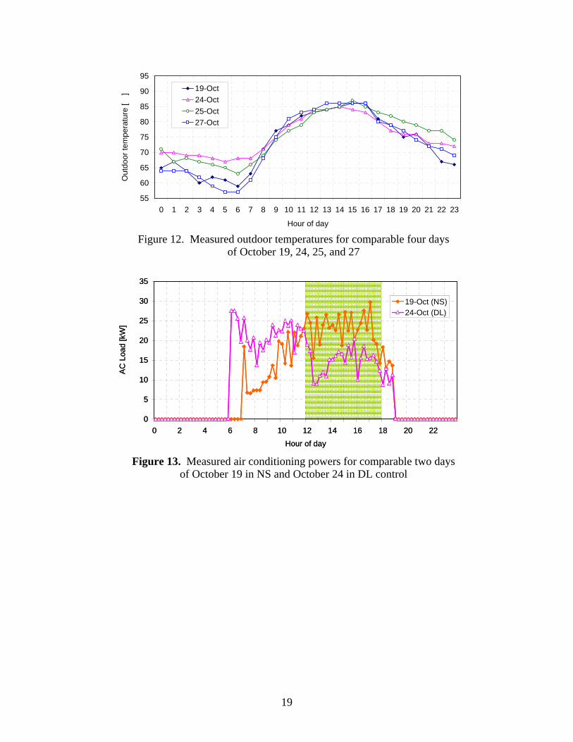
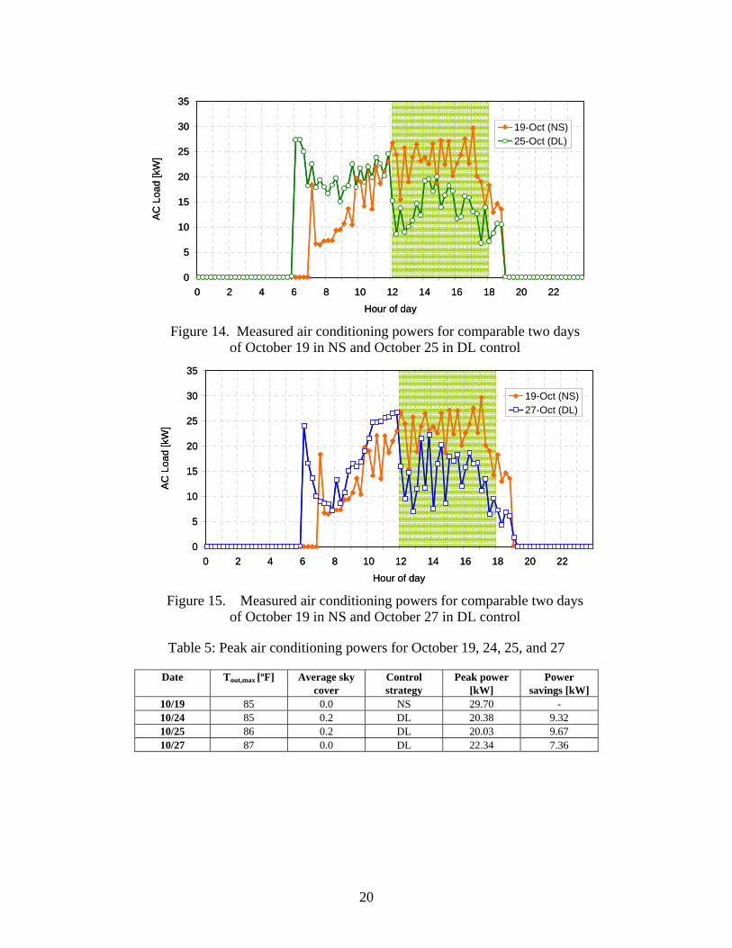
To evaluate performance of the DL strategy for three days (10/24, 10/25, and 10/27)
during the second week testing, October 19 was selected for the baseline case. Measured
outdoor temperature for these four days (10/19 in NS, 10/24, 25, and 27 in DL) are
compared in Figure 12. Measured air conditioner power profiles for the four days are
compared in Figures 13 to 15. Peak air conditioner power and peak power savings for
the four days are represented in Table 5 with maximum outdoor temperatures and
average sky covers. Significant cooling load reductions during the on-peak period are
shown for the three days with DL control compared to the baseline with NS control. The
air conditioning load profiles were not as flat as anticipated by the DL control. One of
the major reasons would be the limitation for precision of setpoint temperatures and the
resetting time interval. If setpoints could be adjusted more finely, the air conditioner
power profiles could be flatter.
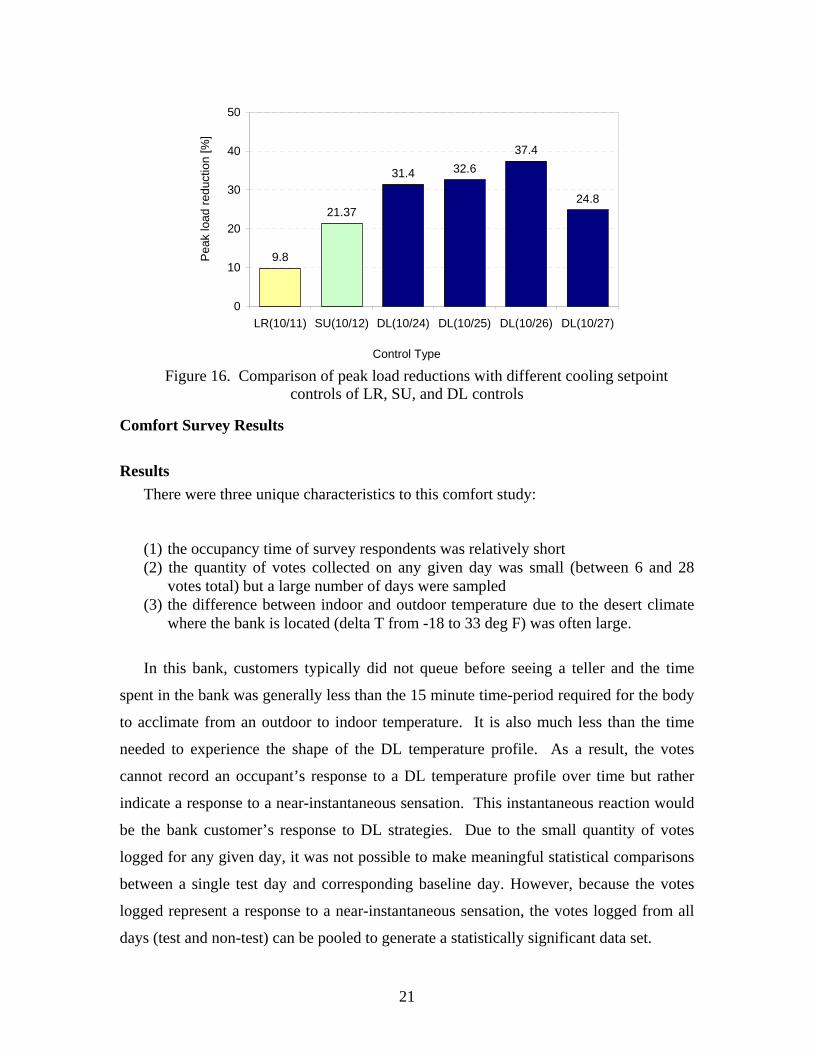
Percent peak air conditioner power savings are compared in Figure 16. Demand-
limiting control with setpoint trajectories determined with the WA method showed better
performance for peak air conditioner power reduction than the simple strategies such as
17
LR and SU. The average peak air conditioner power reduction for the four test days with
DL control was 31.6% as compared with the baseline. The average and maximum of the
peak power savings for the four DL test days were 9.1 and 10.1 kW or 0.76 and
0.84W/ft2.
55
60
65
70
75
80
85
90
95
0 2 4 6 8 10 12 14 16 18 20 22
Hour of day
Out
door
tem
pera
ture
[ �]
9-Oct11-Oct12-Oct
Figure 8. Measured outdoor temperatures for comparable three days
of October 9, 11, and 12
0
5
10
15
20
25
30
0 1 2 3 4 5 6 7 8 9 10 11 12 13 14 15 16 17 18 19 20 21 22 23
Hour of day
AC L
oad
[kW
]
10/9 (NS)10/11 (LR)10/12 (SU)
0
5
10
15
20
25
30
0 1 2 3 4 5 6 7 8 9 10 11 12 13 14 15 16 17 18 19 20 21 22 23
Hour of day
AC L
oad
[kW
]
10/9 (NS)10/11 (LR)10/12 (SU)
Figure 9. Measured air conditioning powers for comparable three days
of October 9, 11, and 12.
Table 3: Peak air conditioning powers for October 9, 11, and 12
Date Tout,max [ºF] Average sky cover
Control strategy
Peak power [kW]
Power savings [kW]
10/9 90 0 NS 26.10 - 10/11 89 0.1 LR 23.53 2.57 10/12 91 0.1 SU 20.52 5.58
18
55
60
65
70
75
80
85
90
95
0 1 2 3 4 5 6 7 8 9 10 11 12 13 14 15 16 17 18 19 20 21 22 23
Hour of day
Out
door
tem
pera
ture
[ �]
17-Oct26-Oct
Figure 10. Measured outdoor temperatures for comparable two days
of October 17 and 26
0
5
10
15
20
25
30
35
0 2 4 6 8 10 12 14 16 18 20 22Hour of day
AC
Loa
d [k
W]
17-Oct (NS)26-Oct (DL)
0
5
10
15
20
25
30
35
0 2 4 6 8 10 12 14 16 18 20 22Hour of day
AC
Loa
d [k
W]
17-Oct (NS)26-Oct (DL)
Figure 11. Measured air conditioning powers for comparable two days
of October 17 in NS and October 26 in DL control
Table 4: Peak air conditioning powers for October 9, 11, and 12
Date Tout,max [ºF] Average sky cover
Control strategy
Peak power [kW]
Power savings [kW]
10/17 80 0.2 NS 27.04 - 10/26 80 0.0 DL 16.94 10.10
19
55
60
65
70
75
80
85
90
95
0 1 2 3 4 5 6 7 8 9 10 11 12 13 14 15 16 17 18 19 20 21 22 23
Hour of day
Out
door
tem
pera
ture
[ �] 19-Oct
24-Oct25-Oct27-Oct
Figure 12. Measured outdoor temperatures for comparable four days
of October 19, 24, 25, and 27
0
5
10
15
20
25
30
35
0 2 4 6 8 10 12 14 16 18 20 22Hour of day
AC L
oad
[kW
]
19-Oct (NS)24-Oct (DL)
0
5
10
15
20
25
30
35
0 2 4 6 8 10 12 14 16 18 20 22Hour of day
AC L
oad
[kW
]
19-Oct (NS)24-Oct (DL)
Figure 13. Measured air conditioning powers for comparable two days
of October 19 in NS and October 24 in DL control
20
0
5
10
15
20
25
30
35
0 2 4 6 8 10 12 14 16 18 20 22Hour of day
AC L
oad
[kW
]
19-Oct (NS)25-Oct (DL)
0
5
10
15
20
25
30
35
0 2 4 6 8 10 12 14 16 18 20 22Hour of day
AC L
oad
[kW
]
19-Oct (NS)25-Oct (DL)
Figure 14. Measured air conditioning powers for comparable two days
of October 19 in NS and October 25 in DL control
0
5
10
15
20
25
30
35
0 2 4 6 8 10 12 14 16 18 20 22Hour of day
AC L
oad
[kW
]
19-Oct (NS)27-Oct (DL)
0
5
10
15
20
25
30
35
0 2 4 6 8 10 12 14 16 18 20 22Hour of day
AC L
oad
[kW
]
19-Oct (NS)27-Oct (DL)
Figure 15. Measured air conditioning powers for comparable two days
of October 19 in NS and October 27 in DL control
Table 5: Peak air conditioning powers for October 19, 24, 25, and 27
Date Tout,max [ºF] Average sky cover
Control strategy
Peak power [kW]
Power savings [kW]
10/19 85 0.0 NS 29.70 - 10/24 85 0.2 DL 20.38 9.32 10/25 86 0.2 DL 20.03 9.67 10/27 87 0.0 DL 22.34 7.36
21
9.8
21.37
31.4 32.637.4
24.8
0
10
20
30
40
50
LR(10/11) SU(10/12) DL(10/24) DL(10/25) DL(10/26) DL(10/27)
Control Type
Pea
k lo
ad re
duct
ion
[%]
Figure 16. Comparison of peak load reductions with different cooling setpoint
controls of LR, SU, and DL controls
Comfort Survey Results
Results There were three unique characteristics to this comfort study:
(1) the occupancy time of survey respondents was relatively short (2) the quantity of votes collected on any given day was small (between 6 and 28
votes total) but a large number of days were sampled (3) the difference between indoor and outdoor temperature due to the desert climate
where the bank is located (delta T from -18 to 33 deg F) was often large.
In this bank, customers typically did not queue before seeing a teller and the time
spent in the bank was generally less than the 15 minute time-period required for the body
to acclimate from an outdoor to indoor temperature. It is also much less than the time
needed to experience the shape of the DL temperature profile. As a result, the votes
cannot record an occupant’s response to a DL temperature profile over time but rather
indicate a response to a near-instantaneous sensation. This instantaneous reaction would
be the bank customer’s response to DL strategies. Due to the small quantity of votes
logged for any given day, it was not possible to make meaningful statistical comparisons
between a single test day and corresponding baseline day. However, because the votes
logged represent a response to a near-instantaneous sensation, the votes logged from all
days (test and non-test) can be pooled to generate a statistically significant data set.
22
Goal
The goal of our analysis was to define setpoint boundaries for an acceptable
percentage of thermal discomfort for comparison with the upper and lower setpoint
bounds implemented in the DL tests (pre-cool to 70 deg F, warming to upper bound of 78
deg F). A further goal was to examine if the difference between indoor and outdoor
temperature influenced customers’ tolerance of the indoor temperature.
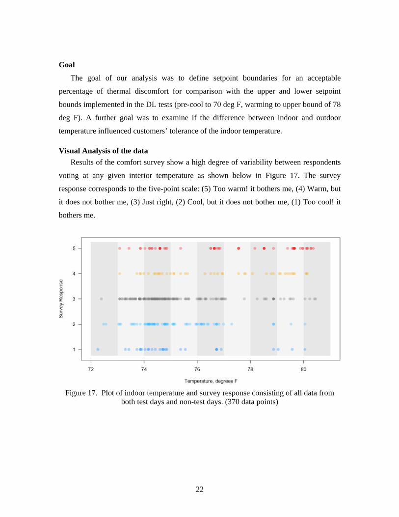
Visual Analysis of the data Results of the comfort survey show a high degree of variability between respondents
voting at any given interior temperature as shown below in Figure 17. The survey
response corresponds to the five-point scale: (5) Too warm! it bothers me, (4) Warm, but
it does not bother me, (3) Just right, (2) Cool, but it does not bother me, (1) Too cool! it
bothers me.
Figure 17. Plot of indoor temperature and survey response consisting of all data from
both test days and non-test days. (370 data points)
23
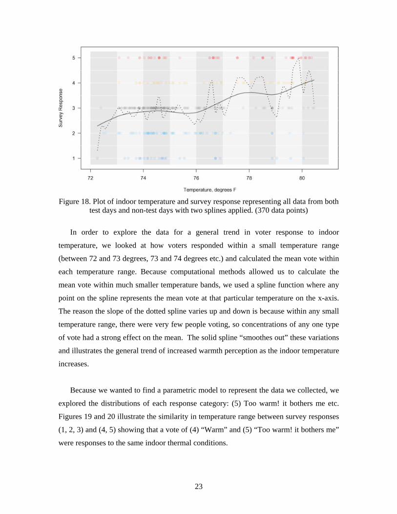
Figure 18. Plot of indoor temperature and survey response representing all data from both
test days and non-test days with two splines applied. (370 data points)
In order to explore the data for a general trend in voter response to indoor
temperature, we looked at how voters responded within a small temperature range
(between 72 and 73 degrees, 73 and 74 degrees etc.) and calculated the mean vote within
each temperature range. Because computational methods allowed us to calculate the
mean vote within much smaller temperature bands, we used a spline function where any
point on the spline represents the mean vote at that particular temperature on the x-axis.
The reason the slope of the dotted spline varies up and down is because within any small
temperature range, there were very few people voting, so concentrations of any one type
of vote had a strong effect on the mean. The solid spline “smoothes out” these variations
and illustrates the general trend of increased warmth perception as the indoor temperature
increases.
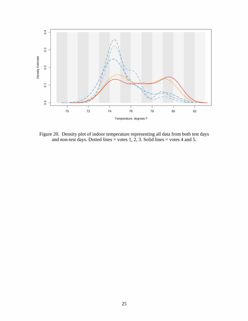
Because we wanted to find a parametric model to represent the data we collected, we
explored the distributions of each response category: (5) Too warm! it bothers me etc.
Figures 19 and 20 illustrate the similarity in temperature range between survey responses
(1, 2, 3) and (4, 5) showing that a vote of (4) “Warm” and (5) “Too warm! it bothers me”
were responses to the same indoor thermal conditions.
24
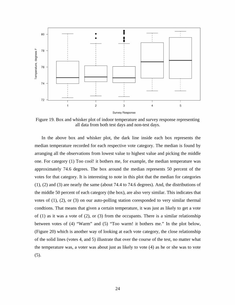
Figure 19. Box and whisker plot of indoor temperature and survey response representing
all data from both test days and non-test days.
In the above box and whisker plot, the dark line inside each box represents the
median temperature recorded for each respective vote category. The median is found by
arranging all the observations from lowest value to highest value and picking the middle
one. For category (1) Too cool! it bothers me, for example, the median temperature was
approximately 74.6 degrees. The box around the median represents 50 percent of the
votes for that category. It is interesting to note in this plot that the median for categories
(1), (2) and (3) are nearly the same (about 74.4 to 74.6 degrees). And, the distributions of
the middle 50 percent of each category (the box), are also very similar. This indicates that
votes of (1), (2), or (3) on our auto-polling station coresponded to very similar thermal
condtions. That means that given a certain temperature, it was just as likely to get a vote
of (1) as it was a vote of (2), or (3) from the occupants. There is a similar relationship
between votes of (4) “Warm” and (5) “Too warm! it bothers me.” In the plot below,
(Figure 20) which is another way of looking at each vote category, the close relationship
of the solid lines (votes 4, and 5) illustrate that over the course of the test, no matter what
the temperature was, a voter was about just as likely to vote (4) as he or she was to vote
(5).
25
Figure 20. Density plot of indoor temperature representing all data from both test days and non-test days. Dotted lines = votes 1, 2, 3. Solid lines = votes 4 and 5.
26
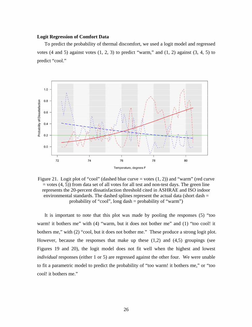
Logit Regression of Comfort Data To predict the probability of thermal discomfort, we used a logit model and regressed
votes (4 and 5) against votes (1, 2, 3) to predict “warm,” and (1, 2) against (3, 4, 5) to
predict “cool.”
Figure 21. Logit plot of “cool” (dashed blue curve = votes (1, 2)) and “warm” (red curve
= votes (4, 5)) from data set of all votes for all test and non-test days. The green line represents the 20-percent dissatisfaction threshold cited in ASHRAE and ISO indoor environmental standards. The dashed splines represent the actual data (short dash =
probability of “cool”, long dash = probability of “warm”)
It is important to note that this plot was made by pooling the responses (5) “too
warm! it bothers me” with (4) “warm, but it does not bother me” and (1) “too cool! it
bothers me,” with (2) “cool, but it does not bother me.” These produce a strong logit plot.
However, because the responses that make up these (1,2) and (4,5) groupings (see
Figures 19 and 20), the logit model does not fit well when the highest and lowest
individual responses (either 1 or 5) are regressed against the other four. We were unable
to fit a parametric model to predict the probability of “too warm! it bothers me,” or “too
cool! it bothers me.”
27
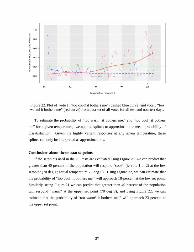
Figure 22. Plot of vote 1: “too cool! it bothers me” (dashed blue curve) and vote 5 “too warm! it bothers me” (red curve) from data set of all votes for all test and non-test days.
To estimate the probability of “too warm! it bothers me,” and “too cool! it bothers
me” for a given temperature, we applied splines to approximate the mean probability of
dissatisfaction. Given the highly variant responses at any given temperature, these
splines can only be interpreted as approximations.
Conclusions about thermostat setpoints
If the setpoints used in the DL tests are evaluated using Figure 21, we can predict that
greater than 40-percent of the population will respond “cool”, (ie vote 1 or 2) at the low
setpoint (70 deg F; actual temperature 72 deg F). Using Figure 22, we can estimate that
the probability of “too cool! it bothers me,” will approach 18-percent at the low set point.
Similarly, using Figure 21 we can predict that greater than 40-percent of the population
will respond “warm” at the upper set point (78 deg F), and using Figure 22, we can
estimate that the probability of “too warm! it bothers me,” will approach 23-percent at
the upper set point.
28
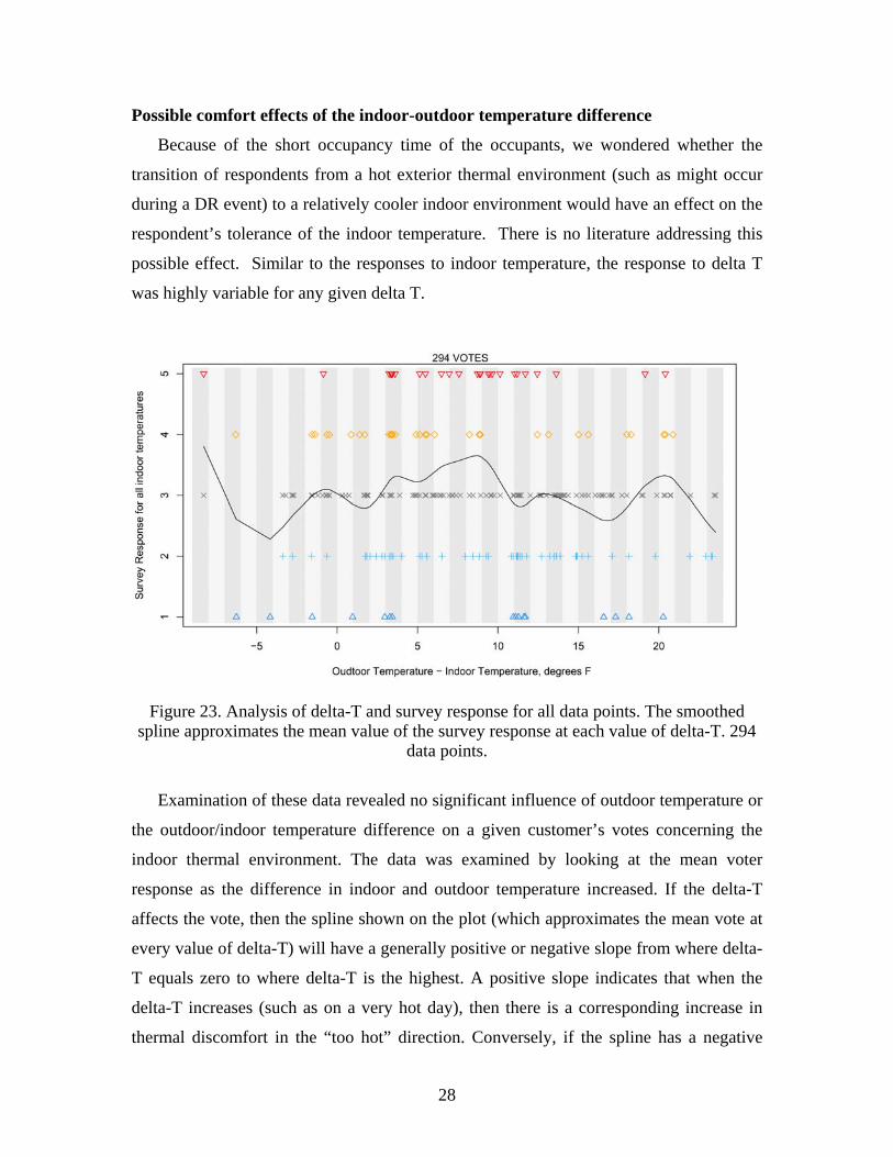
Possible comfort effects of the indoor-outdoor temperature difference
Because of the short occupancy time of the occupants, we wondered whether the
transition of respondents from a hot exterior thermal environment (such as might occur
during a DR event) to a relatively cooler indoor environment would have an effect on the
respondent’s tolerance of the indoor temperature. There is no literature addressing this
possible effect. Similar to the responses to indoor temperature, the response to delta T
was highly variable for any given delta T.
Figure 23. Analysis of delta-T and survey response for all data points. The smoothed
spline approximates the mean value of the survey response at each value of delta-T. 294 data points.
Examination of these data revealed no significant influence of outdoor temperature or
the outdoor/indoor temperature difference on a given customer’s votes concerning the
indoor thermal environment. The data was examined by looking at the mean voter
response as the difference in indoor and outdoor temperature increased. If the delta-T
affects the vote, then the spline shown on the plot (which approximates the mean vote at
every value of delta-T) will have a generally positive or negative slope from where delta-
T equals zero to where delta-T is the highest. A positive slope indicates that when the
delta-T increases (such as on a very hot day), then there is a corresponding increase in
thermal discomfort in the “too hot” direction. Conversely, if the spline has a negative
29
slope, then as the delta-T increases there is a corresponding increase in thermal
discomfort in the “too cold” direction.
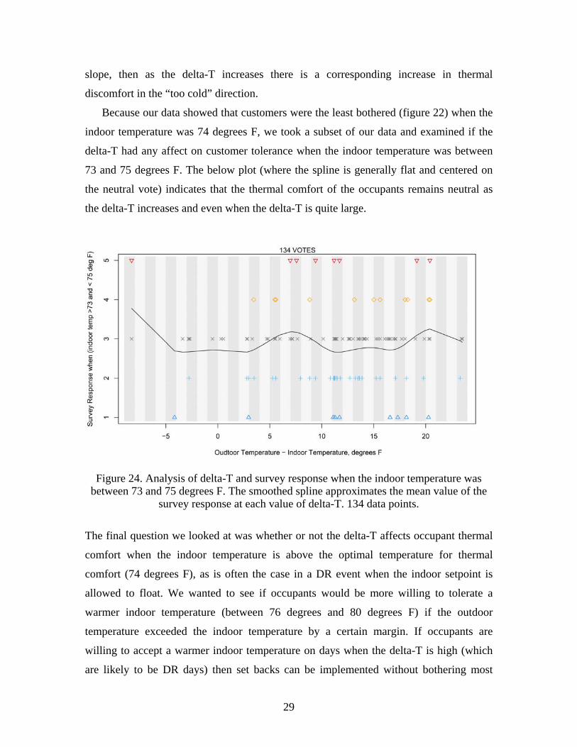
Because our data showed that customers were the least bothered (figure 22) when the
indoor temperature was 74 degrees F, we took a subset of our data and examined if the
delta-T had any affect on customer tolerance when the indoor temperature was between
73 and 75 degrees F. The below plot (where the spline is generally flat and centered on
the neutral vote) indicates that the thermal comfort of the occupants remains neutral as
the delta-T increases and even when the delta-T is quite large.
Figure 24. Analysis of delta-T and survey response when the indoor temperature was
between 73 and 75 degrees F. The smoothed spline approximates the mean value of the survey response at each value of delta-T. 134 data points.
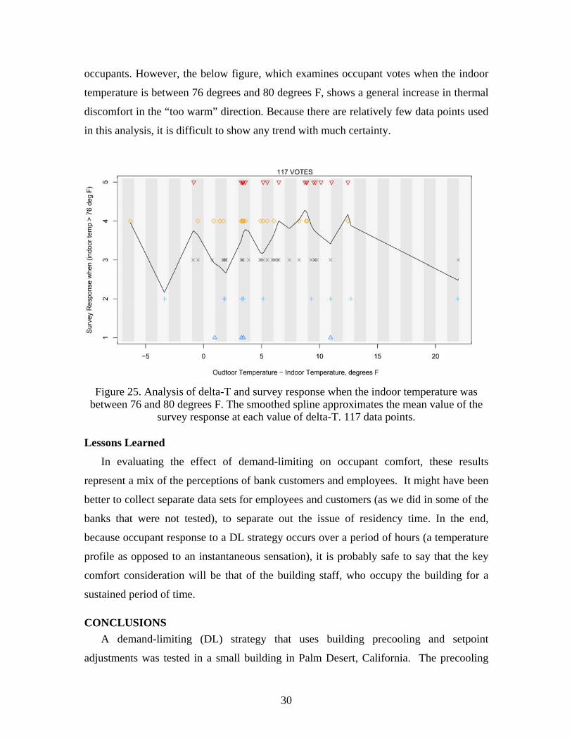
The final question we looked at was whether or not the delta-T affects occupant thermal
comfort when the indoor temperature is above the optimal temperature for thermal
comfort (74 degrees F), as is often the case in a DR event when the indoor setpoint is
allowed to float. We wanted to see if occupants would be more willing to tolerate a
warmer indoor temperature (between 76 degrees and 80 degrees F) if the outdoor
temperature exceeded the indoor temperature by a certain margin. If occupants are
willing to accept a warmer indoor temperature on days when the delta-T is high (which
are likely to be DR days) then set backs can be implemented without bothering most
30
occupants. However, the below figure, which examines occupant votes when the indoor
temperature is between 76 degrees and 80 degrees F, shows a general increase in thermal
discomfort in the “too warm” direction. Because there are relatively few data points used
in this analysis, it is difficult to show any trend with much certainty.
Figure 25. Analysis of delta-T and survey response when the indoor temperature was
between 76 and 80 degrees F. The smoothed spline approximates the mean value of the survey response at each value of delta-T. 117 data points.
Lessons Learned
In evaluating the effect of demand-limiting on occupant comfort, these results
represent a mix of the perceptions of bank customers and employees. It might have been
better to collect separate data sets for employees and customers (as we did in some of the
banks that were not tested), to separate out the issue of residency time. In the end,
because occupant response to a DL strategy occurs over a period of hours (a temperature
profile as opposed to an instantaneous sensation), it is probably safe to say that the key
comfort consideration will be that of the building staff, who occupy the building for a
sustained period of time.
CONCLUSIONS A demand-limiting (DL) strategy that uses building precooling and setpoint
adjustments was tested in a small building in Palm Desert, California. The precooling
31
temperature was set to 70ºF from 6am to 12pm and setpoint temperatures during an on-
peak period from 12pm to 6pm were adjusted from 70ºF to 78ºF. The DL control was
tested for four days in October. The test results indicated that more than 30% reduction
in peak air conditioner load was possible for a 6-hour demand-limiting. The average
peak load savings was 0.76W/ft2 for the test building.
Comfort evaluations were performed for the facility during the field tests, and
baseline data was collected during the days between the tests. The comfort survey
illustrated a highly variable response to the indoor environment on base days as well as
test days. This might be characteristic of buildings such as banks that have a relatively
short customer occupancy time, although this is a new finding. The difference between
outdoor and indoor temperature did not significantly affect customers’ perception of the
indoor temperature. In future studies of buildings that have relatively short customer
occupancy time, it would be useful to collect data from employees rather than customers,
as the employee response to thermal sensation over an extended period of time will better
describe the affect of the thermal profile generated by the DL strategy.
This field test demonstrated that small commercial buildings can be good candidates
for utilization of thermal storage in building mass to reduce peak demands. Additional
work is necessary to thoroughly evaluate the impacts of the strategy on peak load
reduction and comfort of occupants. It would be useful to study the effects of precooling
duration, precooling temperature, comfort temperature range, time interval of setpoint
temperature resetting, and ambient temperature conditions. Furthermore, more small
commercial buildings that have diverse thermal load characteristics should be tested.
In particular, it is important to consider hotter weather. None of the test days
included really hot weather where the cooling loads were high relative to the equipment
cooling capacity. It is expected that hot days would result in similar absolute reductions
in peak power consumption, but lower percentage reductions for use of building thermal
mass as compared with cooler days. It also important to consider comfort impacts for
thermal strategies implemented on hotter days.
Peak power reduction associated with control of building thermal mass could also be
sensitive to the number of air conditioners and stages of capacity control at the site. The
power consumption associated with air conditioning has larger short-term fluctuations
when there are fewer capacity steps due to compressor cycling. Power fluctuations due
32
to on/off cycling of single-stage equipment are evident in the 15-minute data presented in
Figures 9, 11, 13, 14, and 15. Smaller fluctuations would be expected for a larger
building with more air conditioners or if each of the units had multiple stages of control.
Furthermore, lower peak power could be achieved if the run times of the air conditioners
were coordinated.
ACRONYMS
DL demand limiting delta-T temperature difference LR linear rise NS night setup RH relative humidity SU step up WA weighted averaging
REFERENCES
Lee, K.H. and Braun, J.E., 2006a, Model-Based Demand-Limiting Control of Building Thermal Mass, Proceedings of the 2006 System Simulation in Buildings Conference at University of Liege, Liege, Belgium.
Lee, K.-H. and Braun, J.E., 2006b, An Experimental Evaluation of Demand-Limiting Using Building Thermal Mass in a Small Commercial Building, ASHRAE Transactions, vol. 112, pt. 1.
Lee, K.H. and Braun, J.E., 2006c, Development of Methods for Determining Demand-Limiting Setpoint Trajectories in Commercial Buildings Using Short-Term Data Analysis, Proceedings of the 2006 IBPSA-USA Conference at MIT, Boston, MA.
Lee, K.H. and Braun, J.E., 2006d, Evaluation of Methods for Determining Demand-Limiting Setpoint Trajectories in Commercial Buildings Using Short-Term Data Analysis,” Proceedings of the 2006 IBPSA-USA Conference at MIT, Boston, MA.
33
APPENDIX
ENVIRONMENTAL CONDITIONS AND OCCUPANT RESPONSES ON ALL TEST DAYS AND RESPECTIVE BASELINE DAYS
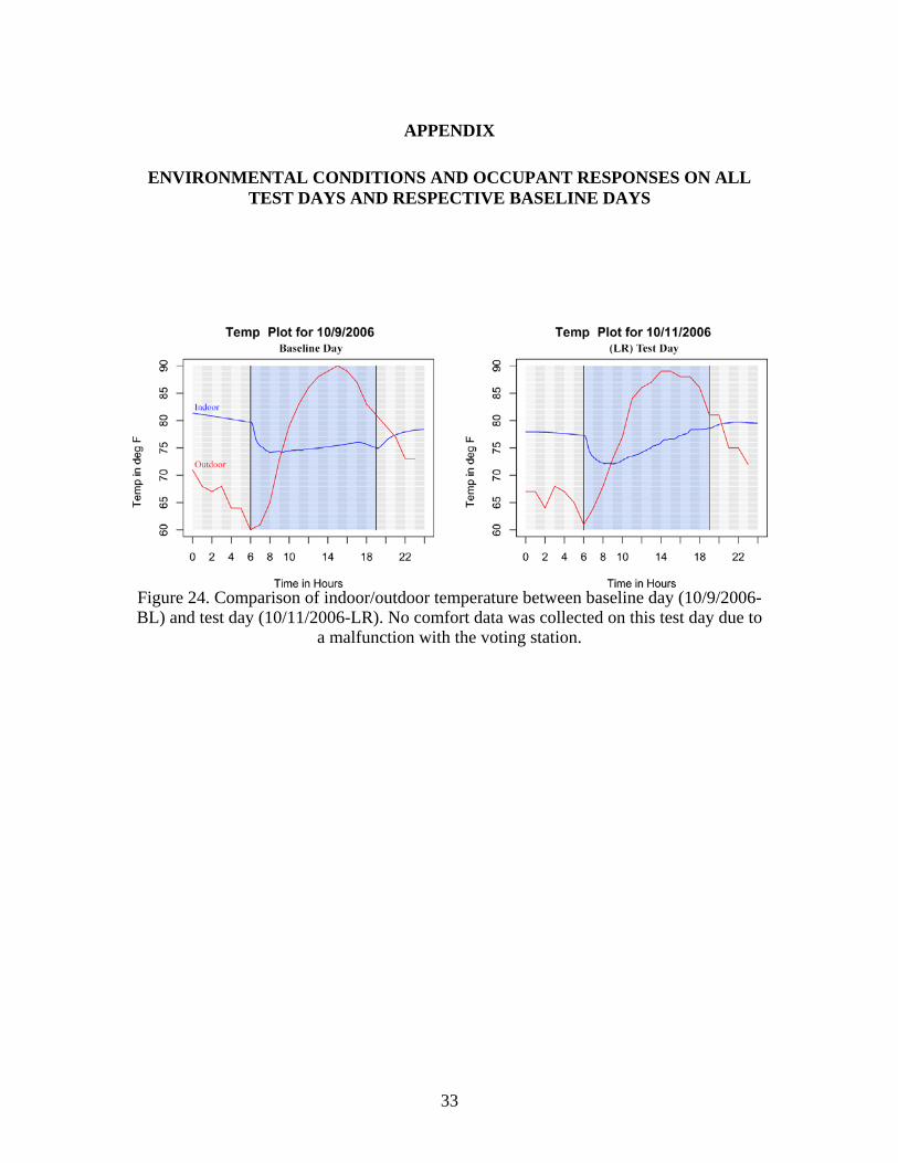
Figure 24. Comparison of indoor/outdoor temperature between baseline day (10/9/2006-BL) and test day (10/11/2006-LR). No comfort data was collected on this test day due to
a malfunction with the voting station.
34
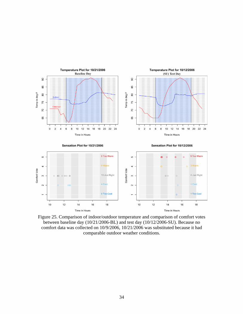
Figure 25. Comparison of indoor/outdoor temperature and comparison of comfort votes
between baseline day (10/21/2006-BL) and test day (10/12/2006-SU). Because no comfort data was collected on 10/9/2006, 10/21/2006 was substituted because it had
comparable outdoor weather conditions.
35
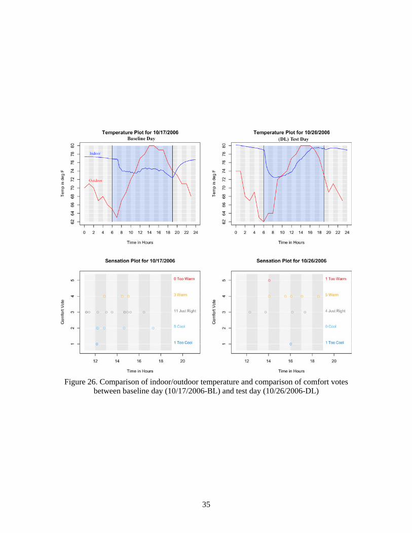
Figure 26. Comparison of indoor/outdoor temperature and comparison of comfort votes
between baseline day (10/17/2006-BL) and test day (10/26/2006-DL)
36
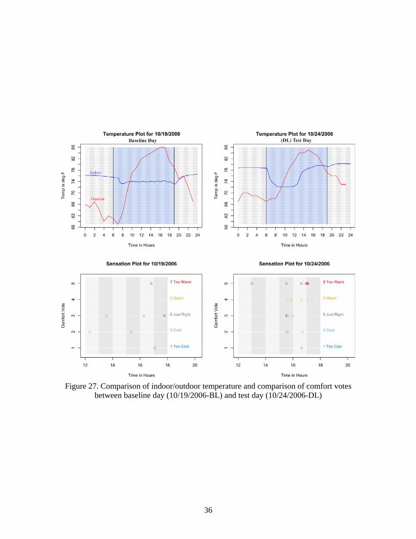
Figure 27. Comparison of indoor/outdoor temperature and comparison of comfort votes
between baseline day (10/19/2006-BL) and test day (10/24/2006-DL)
37
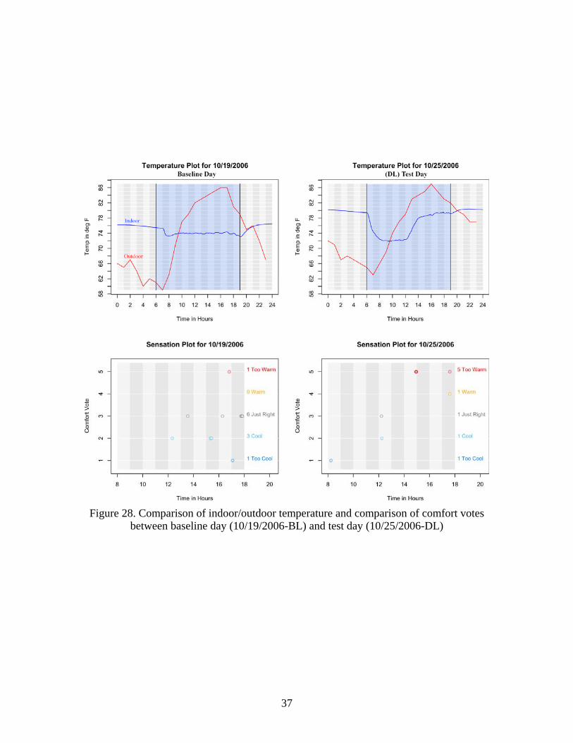
Figure 28. Comparison of indoor/outdoor temperature and comparison of comfort votes
between baseline day (10/19/2006-BL) and test day (10/25/2006-DL)
38
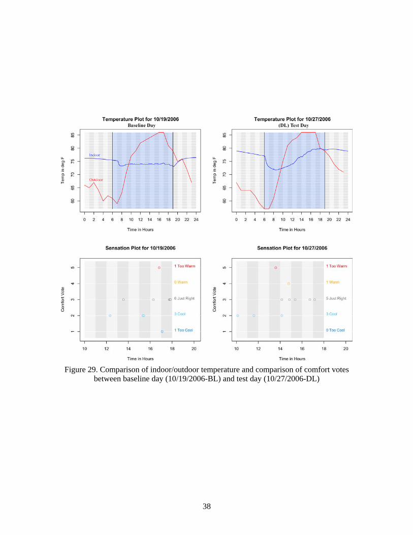
Figure 29. Comparison of indoor/outdoor temperature and comparison of comfort votes
between baseline day (10/19/2006-BL) and test day (10/27/2006-DL)