testing cometary ejection models to fit the 1999 leonids and to predict future showers

Mon. Not. R. Astron. Soc. 317, L1±L5 (2000)

Testing cometary ejection models to fit the 1999 Leonids and to predictfuture showers

C. GoÈckel and R. Jehnw

ESA/ESOC, Robert-Bosch-Str. 5, 64293 Darmstadt, Germany

Accepted 2000 June 9. Received 2000 May 24; in original form 2000 April 19

A B S T R A C T

Brown & Jones have discussed four models for the ejection velocities of cometary material

during the perihelion passage of a comet. The ejection velocities depend on the heliocentric

distance, density and mass of the ejected particle and on the size of the comet. For the

density of the particles, they assumed three values, 100, 800 and 4000 kg m23, which give a

possible combination of 12 cometary ejection models. This paper tests whether these models

can be applied to explain the Leonid phenomenon for which Comet 55P/Tempel±Tuttle is

responsible. The ejection is simulated of 61 000 particles during each of the last four

apparitions of Tempel±Tuttle, and flux rates on Earth are derived. The results prove that the

models with a particle density of 4000 kg m23 provide the best fit to the observed Leonid

rates in 1999. Based on the ejection velocity model that gives the smallest root-mean-square

error for the year 1999, noticeable displays of the Leonids are predicted for 2000 and 2001

November.

Key words: comets: individual: 55P/Tempel±Tuttle ± meteors, meteoroids ± Solar system:

general.

1 I N T R O D U C T I O N

The Leonids are small dust particles which enter the upper

atmosphere of the Earth with a very high velocity of about

71 km s21. They are the result of the passage of the Earth through

dust trails of Comet 55P/Tempel±Tuttle. The meteor activity

associated with Comet Tempel±Tuttle is called a `Leonid' event

because the meteors appear to be coming from the direction of the

constellation Leo. There is evidence that this comet has created

meteor showers and meteor storms for more than 1000 years.

Tempel±Tuttle, named after Ernst Tempel and Horace Tuttle who

first discovered the comet in 1865 and 1866, has a nuclear radius of

about 2 km (Hainaut et al. 1998) and orbits the Sun with a period of

just over 33 yr. At its perihelion it passes close to the orbit of the

Earth. The last perihelion passage occurred on 1998 February 28.

Until recently the capabilities of predicting the time and the

intensity of the Leonids were quite poor. However, new research

studies, especially those performed by Kondrat'eva & Reznikov

(1985), Kondrat'eva, Murav'eva & Reznikov (1997), McNaught

& Asher (1999) and Brown (2000), have provided a better

understanding of the phenomenon of the Leonids. McNaught &

Asher claim that the time of maximum is now predictable to 10-

min accuracy or better.

In this paper the cometary ejection models of Brown & Jones

(1998) are applied in order to simulate the dust population of

Tempel±Tuttle released since 1866 (Section 2). The dust particles

are propagated with a Stumpff±Weiss orbit propagator (Section 3),

and encounters with the Earth in the year 1999 are analysed for all

models (Section 4). Finally in Section 5, predictions for the years

2000 and 2001 are made, based on the model, that best fit the

observational data on the 1999 Leonids.

2 C O M E TA RY E J E C T I O N M O D E L S

When a comet approaches the Sun, sublimation of volatiles

(primarily water ice) sets in, and particles are caused by

momentum transfer to leave the parent comet. Reflecting the

considerable uncertainty about the ejection process, four different

models have been developed by Brown & Jones (1998) to describe

the initial formation of the meteoroid stream. They are based on

Whipple's (1951) `icy snowball' model:

veject � 8:03r21:125r21=3r1=2c m21=6f ;

where r is the heliocentric distance in au, r and m are the density

and mass of the grain, respectively, rc is the radius of the cometary

nucleus and f is the fraction of incident solar radiation used in

sublimation; the latter is set to 1 throughout.

The Whipple formula was slightly changed by (among others)

Jones (1995) to correct the assumption of a blackbody-limited

nucleus temperature as well as the neglect of the adiabatic expansion

of the gas. This corrected formula is chosen as the first model:

veject � 10:2r21:038r21=3r1=2c m21=6:

To allow, furthermore, grains of the same mass but with

q 2000 RAS

w E-mail: [email protected]

different shapes to reach different velocities, a parabolic

distribution is added for the second model:

P�v 2 veject� � 1 2v

veject

2 1

� �2

in the range of 0 , v , 2veject:The Whipple-derived theories, as do many others, suggest a

variation of ejection velocity with heliocentric distance that is of the

form veject / rn; where in the above cases n is close to 21. Since

from observations of coma ejection/halo expansions a value of 20.5

can also be deduced, this possibility is adopted in the third model:

veject � 10:2r20:5r21=3r1=2c m21=6:

For the fourth model a different approach is used. Besides the

surface as the source of meteoroid grains, sublimation and meteoroid

production are now considered to occur throughout the coma. This

concept of `distributed' production in the coma was investigated

by Crifo (1995) in his physicochemical model of the inner coma.

The ejection process can thus be expressed by the formula

log10 v � 22:143 2 0:605 log10�rgrain�2 0:5 log10r;

where rgrain is the radius of the meteoroid grain. Furthermore, the

escape velocity of the particle from the comet has to be subtracted

to obtain the final ejection velocity, which is then used together

with Crifo's distribution for the differential flux:

P�v 2 veject�

� 1

e3:7exp

3:7 2 10:26�v 2 veject� � 4:12�v 2 veject�21 2 1:03�v 2 veject� � 0:296�v 2 veject�2

" #:

A summary of the employed ejection models is given in Table 1.

As can be seen in the above-presented formulae, the ejection

velocity varies as a function of the density and mass of the grains.

To complete the modelling of the ejection process, it is thus

necessary to have a closer look at these parameters. Estimates

regarding the density of meteoroids are widespread and vary

between 100 and 4000 kg m23. To cover this range, Brown &

Jones (1998) used three distinct values of 100, 800 and 4000

kg m23. This means that, instead of the original four models, 12

model variants are now examined. The density is denoted by a

second number appended to the model number: for example,

models 11, 12 and 13 denote the first model with meteoroid

densities of 100, 800 and 4000 kg m23, respectively.

To simulate the ejection of dust grains of different sizes, the

masses of the meteoroids are varied between 1025 and 10 g. Over

this range, 61 mass categories are used, each being 0.1 greater in

log m than the previous one. In each mass category the ejection of

1000 meteoroids is simulated (assuming a logarithmic distribution

in the absence of a better mass function), totalling 61 000 particles

per model and per perihelion passage.

For the ejection activity a limit of 4 au is chosen, accounting for

more volatile compounds than water, since water sublimation fails

at distances of more than 3 au. Hence the ejection process is

considered to start when the comet approaches the Sun to a

distance of less than 4 au. The number of ejected particles depends

upon the amount of incoming solar energy and is thus proportional

to r22. On the other hand, from Kepler's second law it is evident

that the probability for the comet to be at a heliocentric distance r

is proportional to r2. This implies that the number of ejected

particles is uniformly distributed for all values of true anomaly

within the active segment of the cometary orbit.

Additionally, sublimation occurs only on the sunward side of

the cometary surface, and the activity reaches its maximum in the

direction of the Sun, whereas the ejection process decreases

towards the edge of the sunlit area. This is modelled by a cosafactor, where the direction of the ejected particle is described by

its angle a to the comet±Sun line.

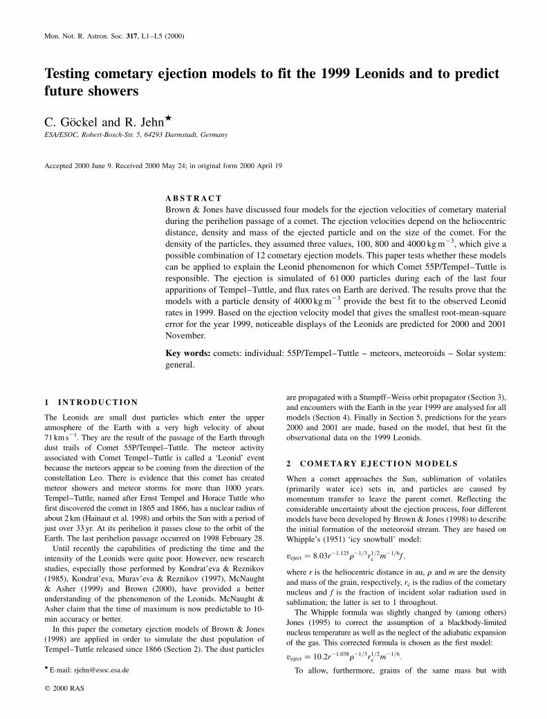
In Fig. 1 the ejection velocity according to the four models is

plotted as function of the heliocentric distance. For this plot, 1000

meteoroids with a density of 800 kg m23 and a mass of 0.01 g

were simulated.

3 T H E N U M E R I C A L I N T E G R AT O R

In order to integrate thousands of particles over more than 100 yr,

a fast but still reliable orbit propagator is needed. Therefore a

Table 1. The formulae for the ejection velocity according to the four model variants. The units are �rgrain� � cm; �r� � au; �rc� � km; �r� � g cm23 and�m� � g to get the ejection velocity in m s21 (Brown & Jones 1998).

Model Name Ejection formulano.

1 Jones ejection distribution veject � 10:2r21:038r21=3r1=2c m21=6

2 Jones ejection distribution with parabolic probability distribution veject � 10:2r21:038r21=3r1=2c m21=6

P�v 2 veject� � 1 2 vveject

2 1� �2

for 0 , v , 2veject

3 Jones ejection distribution with modified heliocentric velocity dependence veject � 10:2r20:5r21=3r1=2c m21=6

4 Crifo distributed production log10�veject � v0� � 22:143 2 0:605 log10�rgrain�2 0:5 log10r

with v20 � 2m=rc and m � GM

P�v 2 veject� � 1e3:7 exp

3:7210:26�v2veject��4:12�v2veject�2121:03�v2veject��0:296�v2veject�2h i

0

10

20

30

40

50

60

70

80

1 1.5 2 2.5 3 3.5 4

Eje

ctio

nve

loci

ty(m

/s)

r (AU)

Model 1Model 2Model 3Model 4

Figure 1. Ejection velocity distributions as a function of heliocentric

distance according to the four models. For each model, 1000 meteoroids

were simulated with a mass of 0.01 g and a density of 800 kg m23.

L2 C. GoÈckel and R. Jehn

q 2000 RAS, MNRAS 317, L1±L5

Stumpff±Weiss orbit generator was chosen (Stumpff & Weiss

1968). In the Stumpff±Weiss method the solution of the N-body

problem is computed as a linear combination of elementary

Keplerian orbits for all the possible couples of bodies, providing a

fourth-order approximation of state and a third-order approxima-

tion of velocity, although higher orders are attainable by

integrating the acceleration remainders. For this method, the

formulation is symmetrical with respect to all the bodies

irrespective of their gravitational influence and, consequently,

the concepts of sphere of influence and of central body are no

longer used and it is not necessary to reformulate the equations

during the integration.

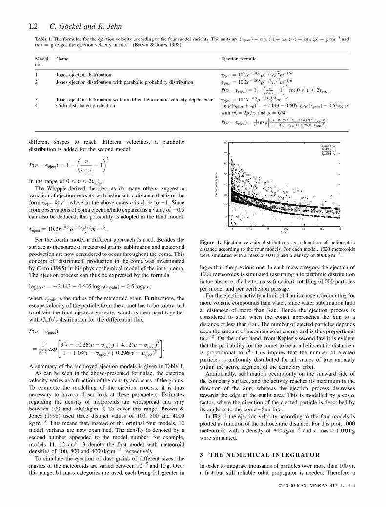
The Stumpff±Weiss orbit generator has been used to propagate

Comet Tempel±Tuttle backward in time, taking into account the

gravitational perturbations caused by Earth, Mars, Jupiter, Saturn

and Uranus. The major perturbations are due to Jupiter. Fig. 2

shows the minimum distances between the comet and the orbit of

Earth at the time of passage of the comet through its descending

node. The results are identical to those of Yeomans (1998). Close

approaches can be seen in the years 1833 and 1966. In both years

the Leonids gave a spectacular display.

The effects of solar radiation pressure, which are increasingly

dominant with decreasing particle size, are taken into account by

adjusting the position and the velocity of the particle after each

integration step (Prieto-Llanos 1985). Tests with a Runge±Kutta

integrator of order 7/8 have revealed that the inclusion of solar

radiation pressure introduces a systematic bias. GoÈckel (2000),

therefore, has introduced a size-dependent correction factor which

reduces the effect of the solar radiation pressure and reduces the

difference between the two orbit propagators to an acceptable

level.

4 B E S T M O D E L T O F I T T H E O B S E RVAT I O N S

O F 1 9 9 9

After intensive testing of the orbit propagator, the orbits of the

ejected particles have been calculated. First the comet is integrated

backward in time, so that meteoroids can be ejected during the last

perihelion passages of the comet. The last perihelion passage

occurred in 1998, and every 33 yr before that. 1866 has been

chosen as the beginning of our simulations, since the results of

Kondrat'eva et al. (1997), McNaught & Asher (1999) and Brown

(2000) have shown that previous returns did not actually

contribute to the 1999 Leonids. Thus 61 000 meteoroids per

model have been ejected around the years 1866, 1899, 1932 and

1965 under the conditions described in Section 2.

Since only very few simulated meteoroids would actually hit

the Earth, and constraints arising from computer power limit their

total number, it has been found necessary to adopt a temporal and

spatial `smearing' to get useful results. This means that particles

passing the Earth at a small distance are also regarded as hits.

Regarding the choice of this maximum miss distance, the reader is

referred to Brown (2000) who suggested a spatial deviation of

0.001 au and a temporal deviation of 0.02 yr (about 1 week) to be

appropriate. The same spatial deviation has been adopted, but the

temporal deviation has been reduced to 0.01 yr. Hence a particle

with a descending node ± which marks its minimal distance to the

Earth ± that lies within 0.001 au of the orbit of the Earth is

counted as a hit, provided that the Earth passes the descending

node of the particle within half a week before or after the particle

itself reached this point. The closer the particle passes to the Earth,

the higher weight it has in the simulated flux rate. The weight

function is

f �x; y� � �0:001 2 x��3:6524 2 y�;

where x is the spatial and y the temporal distance between the

particle and the Earth in units of au and days, respectively.

Furthermore, a triangular function is attributed to each impacting

particle, where the height of the triangle is determined by the

weight of the hit described above, and the width of its base is fixed

to 08: 05 of solar longitude. The latter causes the location of the hit

to be smeared out over a duration of 1.2 h ± which is what it takes

the Earth to pass 08: 05 of solar longitude. All hits are summed over

the time or solar longitude.

The predicted meteor rates have to be compared with the

-0.025

-0.02

-0.015

-0.01

-0.005

0

0.005

0.01

0.015

1600 1650 1700 1750 1800 1850 1900 1950 2000 2050 2100

Com

et-E

arth

Orb

italS

epar

atio

nD

ista

nce

(AU

)

Time (calendar year)

Stumpff-Weiss orbit propagatorYeomans

Figure 2. Minimum distances between Comet Tempel±Tuttle and the orbit

of the Earth at the time of the comet's passage through its descending

node. The Stumpff±Weiss orbit propagator gives identical results to those

calculated by Yeomans (1998).

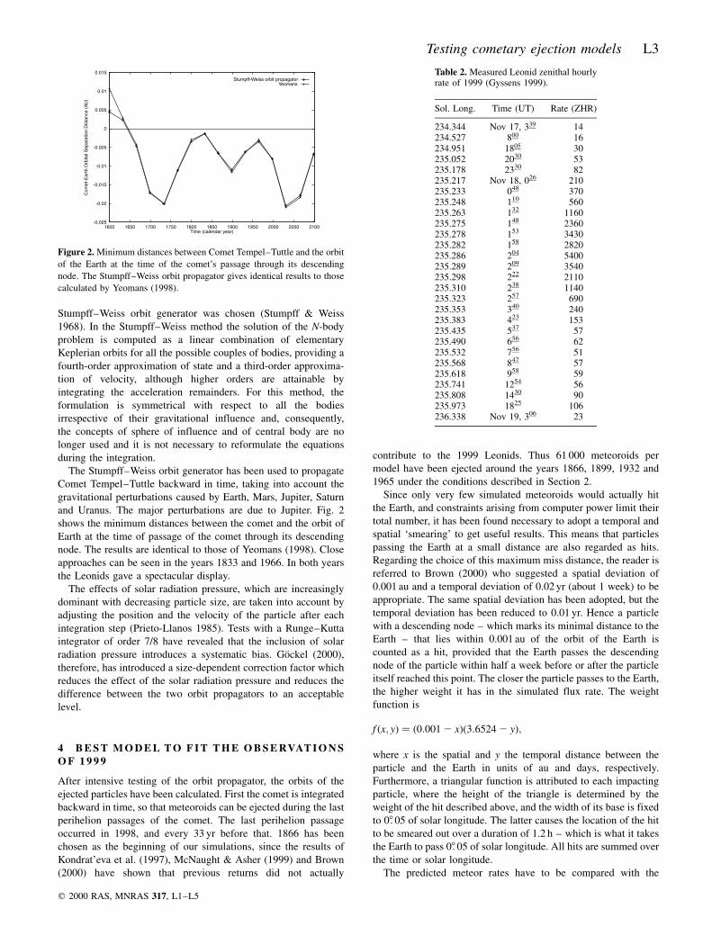
Table 2. Measured Leonid zenithal hourlyrate of 1999 (Gyssens 1999).

Sol. Long. Time (UT) Rate (ZHR)

234.344 Nov 17, 339 14234.527 800 16234.951 1805 30235.052 2030 53235.178 2330 82235.217 Nov 18, 026 210235.233 048 370235.248 110 560235.263 132 1160235.275 148 2360235.278 153 3430235.282 158 2820235.286 204 5400235.289 209 3540235.298 222 2110235.310 238 1140235.323 257 690235.353 340 240235.383 423 153235.435 537 57235.490 656 62235.532 756 51235.568 847 57235.618 958 59235.741 1254 56235.808 1430 90235.973 1825 106236.338 Nov 19, 306 23

Testing cometary ejection models L3

q 2000 RAS, MNRAS 317, L1±L5

measured Leonid rate of 1999 (Table 2), so that a ranking of the

models can be made. For this purpose the 12 simulated curves are

first scaled by a factor of 500 so that they match the order of

magnitude of the measured Leonid zenithal hourly rate, and then

the method of least squares is applied. This yields the numbers

shown in Table 3, where the models are ordered by their root-

mean-square residual between the simulated and measured Leonid

rates of 1999.

The best fit to the observed data is achieved with model 43. As

can also be seen in Table 3, the models with a higher density of the

meteoroids (end-number `3') fit better than those with lower

densities. The models assuming a particle density of 100 kg m23

(end-number `1') provide the worst fit. This means that the

ejection velocity distribution has less influence on the evolution of

the dust trails than does the particle density which dictates the

effects of the solar radiation pressure. This is confirmed by

Lyytinen's simulations (1999) which show evolution of the dust

trails that is very similar to our results, although extremely low

ejection velocities are assumed (1 m s21 and lower).

In Fig. 3 the Leonid rate is presented for the year 1999 as

simulated with model 43. A closer look reveals that the peak in the

meteor rate is caused by particles that were ejected in the periods

of 1899 and 1932, whereas the secondary peaks around a solar

longitude of 2358: 8 are due to particles ejected in 1866. This is in

agreement with the other models, too. In Fig. 4 the dust clouds of

particles ejected in different periods are plotted for the time when

they cross the ecliptic plane in 1999 mid-November, based on

model 43. The positions of the dust clouds with respect to each

other can be seen. In 1999 the Earth is going directly through the

clouds of 1899 and 1932 and ± half a day later ± through the dust

cloud ejected in 1866. This explains the spectacular high Leonid

peak observed in 1999. These results are in good agreement with

the results of McNaught & Asher (1999). A nice graphical

presentation showing the trajectory of the Earth passing through

(or by) the particle trails of the individual ejection periods is given

by Asher (2000). It can also be found on the website of Armagh

Observatory at http://www.arm.ac.uk/leonid/dustexpl.html.

5 P R E D I C T I O N S F O R T H E Y E A R S 2 0 0 0 A N D

2 0 0 1

Since the models with a high particle density give the best fit of

the observed Leonid rates in the year 1999, they are applied to

predict the date, time and activity level of the Leonid showers in

the years 2000 and 2001. The maximum in the year 2000 is

expected to take place at a solar longitude around 2358: 27. Models

13, 33 and 43 predict the peak to be between 07:30 and 08:20 ut

on 2000 November 17 with a secondary peak 24 h later. The

activity level for model 43 is nearly half as high as in 1999, as can

be seen in Fig. 5. Fig. 6 reveals that this peak at a solar longitude

of 2358: 27 is caused by particles ejected in 1932, whereas the

secondary peak is caused by `1866 particles'. The particles ejected

in 1899 which were mainly responsible for the storm in 1999 are

no longer dominant. This is in perfect agreement with the results

from Kondrat'eva et al. (1997), Lyytinen (1999) and McNaught &

Asher (1999), who included ejection of cometary material even

back to the year 1733. According to their simulations, the Earth

will pass through the cloud of `1733 particles' in the early

morning hours of 2000 November 18.

According to our simulations, the activity will further decrease

in the year 2001. Fig. 7 shows that the activity may reach less than

Table 3. Ordering of the modelsaccording to the root-mean-squareresidual between simulated andmeasured Leonid rates of 1999. Thefirst number of the model variantindicates the ejection velocity modelas described in Table 1, and thesecond number indicates the particledensity (1: 100 kg m23, 2: 800 kgm23, 3: 4000 kg m23).

Model RMS residual (�108)

1 43 1.851 91112 13 3.256 29763 33 3.341 15414 22 4.077 21935 42 4.161 13996 23 4.344 43747 32 4.634 47128 12 4.714 41949 31 4.716 2975

10 11 5.362 864311 41 5.843 830012 21 5.852 9747

0

0.5

1

1.5

2

2.5

3

3.5

4

4.5

234.4 234.6 234.8 235 235.2 235.4 235.6 235.8 236 236.2 236.4

Met

eor

rate

1999

Solar longitude (deg)

Model 43

SumEjected 1866Ejected 1899Ejected 1932

Figure 3. The simulated Leonid rate in the year 1999 for model 43. Note

that the measured Leonid peak of 1999 (Table 2) occurred at a solar

longitude of 2358: 286. The position of the maximum of the above curve

coincides perfectly with this value.

1.18e+08

1.19e+08

1.2e+08

1.21e+08

1.22e+08

1.23e+08

1.24e+08

1.25e+08

1.26e+08

1.27e+08

7.6e+07 7.8e+07 8e+07 8.2e+07 8.4e+07 8.6e+07 8.8e+07 9e+07

y(k

m)

x (km)

1999

Nov 21

Nov 20

Nov 19

Nov 17

Nov 16

Earth orbit1866189919321965

Figure 4. The descending nodes of particles crossing the ecliptic plane in

the year 1999 one week before or after the Earth passed the point of

minimum distance (as simulated with model 43). The ejection years of the

particles are indicated by different symbols, and thus it becomes clear

which ejection periods were mainly responsible for the Leonid storm in

1999. The line marks the orbit of the Earth with labels indicating the date

(midnight) when the Earth reached the corresponding position.

L4 C. GoÈckel and R. Jehn

q 2000 RAS, MNRAS 317, L1±L5

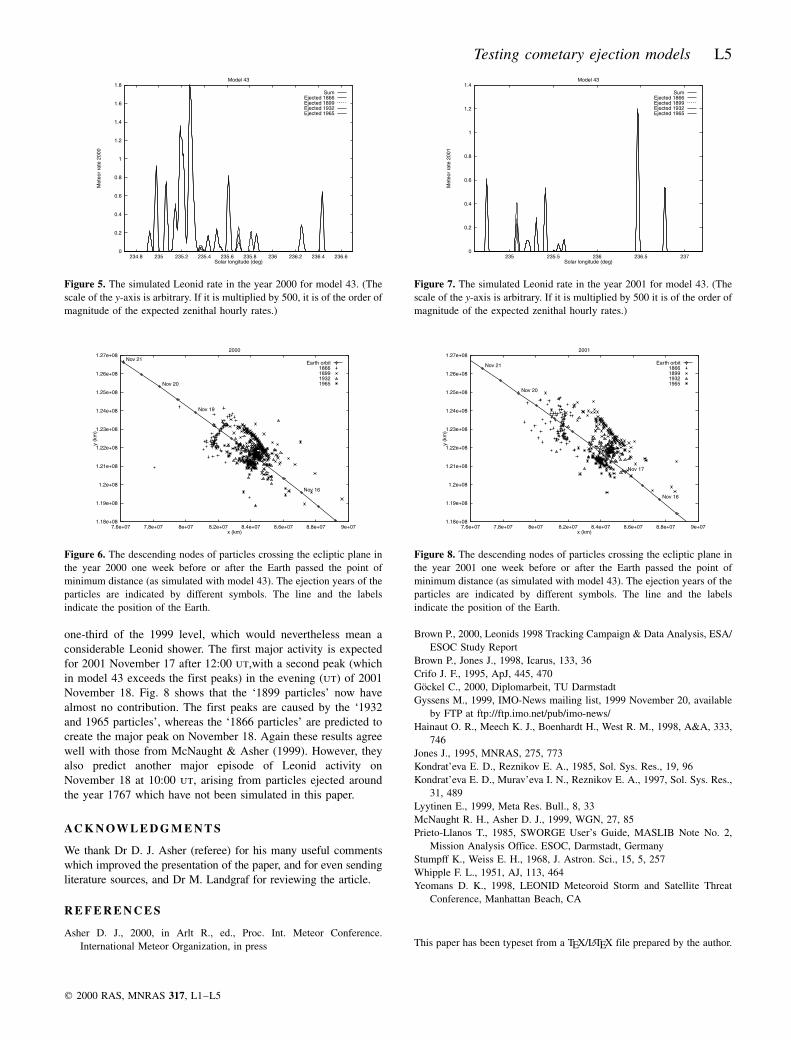
one-third of the 1999 level, which would nevertheless mean a

considerable Leonid shower. The first major activity is expected

for 2001 November 17 after 12:00 ut,with a second peak (which

in model 43 exceeds the first peaks) in the evening (ut) of 2001

November 18. Fig. 8 shows that the `1899 particles' now have

almost no contribution. The first peaks are caused by the `1932

and 1965 particles', whereas the `1866 particles' are predicted to

create the major peak on November 18. Again these results agree

well with those from McNaught & Asher (1999). However, they

also predict another major episode of Leonid activity on

November 18 at 10:00 ut, arising from particles ejected around

the year 1767 which have not been simulated in this paper.

AC K N OW L E D G M E N T S

We thank Dr D. J. Asher (referee) for his many useful comments

which improved the presentation of the paper, and for even sending

literature sources, and Dr M. Landgraf for reviewing the article.

R E F E R E N C E S

Asher D. J., 2000, in Arlt R., ed., Proc. Int. Meteor Conference.

International Meteor Organization, in press

Brown P., 2000, Leonids 1998 Tracking Campaign & Data Analysis, ESA/

ESOC Study Report

Brown P., Jones J., 1998, Icarus, 133, 36

Crifo J. F., 1995, ApJ, 445, 470

GoÈckel C., 2000, Diplomarbeit, TU Darmstadt

Gyssens M., 1999, IMO-News mailing list, 1999 November 20, available

by FTP at ftp://ftp.imo.net/pub/imo-news/

Hainaut O. R., Meech K. J., Boenhardt H., West R. M., 1998, A&A, 333,

746

Jones J., 1995, MNRAS, 275, 773

Kondrat'eva E. D., Reznikov E. A., 1985, Sol. Sys. Res., 19, 96

Kondrat'eva E. D., Murav'eva I. N., Reznikov E. A., 1997, Sol. Sys. Res.,

31, 489

Lyytinen E., 1999, Meta Res. Bull., 8, 33

McNaught R. H., Asher D. J., 1999, WGN, 27, 85

Prieto-Llanos T., 1985, SWORGE User's Guide, MASLIB Note No. 2,

Mission Analysis Office. ESOC, Darmstadt, Germany

Stumpff K., Weiss E. H., 1968, J. Astron. Sci., 15, 5, 257

Whipple F. L., 1951, AJ, 113, 464

Yeomans D. K., 1998, LEONID Meteoroid Storm and Satellite Threat

Conference, Manhattan Beach, CA

This paper has been typeset from a TEX/LATEX file prepared by the author.

0

0.2

0.4

0.6

0.8

1

1.2

1.4

1.6

1.8

234.8 235 235.2 235.4 235.6 235.8 236 236.2 236.4 236.6

Met

eor

rate

2000


Model 43

SumEjected 1866Ejected 1899Ejected 1932Ejected 1965

Figure 5. The simulated Leonid rate in the year 2000 for model 43. (The

scale of the y-axis is arbitrary. If it is multiplied by 500, it is of the order of

magnitude of the expected zenithal hourly rates.)

1.18e+08

1.19e+08

1.2e+08

1.21e+08

1.22e+08

1.23e+08

1.24e+08

1.25e+08

1.26e+08

1.27e+08

7.6e+07 7.8e+07 8e+07 8.2e+07 8.4e+07 8.6e+07 8.8e+07 9e+07

y(k

m)

x (km)

2000

Nov 21

Nov 20

Nov 19

Nov 16

Earth orbit1866189919321965




particles are indicated by different symbols. The line and the labels

indicate the position of the Earth.

0

0.2

0.4

0.6

0.8

1

1.2

1.4

235 235.5 236 236.5 237

Met

eor

rate

2001


Model 43

SumEjected 1866Ejected 1899Ejected 1932Ejected 1965

Figure 7. The simulated Leonid rate in the year 2001 for model 43. (The

scale of the y-axis is arbitrary. If it is multiplied by 500 it is of the order of

magnitude of the expected zenithal hourly rates.)

1.18e+08

1.19e+08

1.2e+08

1.21e+08

1.22e+08

1.23e+08

1.24e+08

1.25e+08

1.26e+08

1.27e+08

7.6e+07 7.8e+07 8e+07 8.2e+07 8.4e+07 8.6e+07 8.8e+07 9e+07

y(k

m)

x (km)

2001

Nov 21

Nov 20

Nov 17

Nov 16

Earth orbit1866189919321965




particles are indicated by different symbols. The line and the labels

indicate the position of the Earth.

Testing cometary ejection models L5

q 2000 RAS, MNRAS 317, L1±L5

testing cometary ejection models to fit the 1999 leonids and to predict future showers

Documents