Temporal dynamics of total organic carbon export rates in Swedish streams

Importance of discharge conditions and

seasonal effects

Nino Amvrosiadi

May, 2012

Copyright © Nino Amvrosiadi and the Department of Earth Sciences, Uppsala University

i

To my father

ii

Abstract

Temporal dynamics of total organic carbon export rates in Swedish streams – Importance of discharge conditions and seasonal effects

Nino Amvrosiadi Department of Earth Sciences, Uppsala University Villavägen 16, SE-752 36 Uppsala, Sweden

The amount of total organic carbon (TOC) in water is a rough indicator of the water quality. Driven by the question how the TOC concentration would vary across streams in Sweden under different climate conditions (e.g. more extreme discharge events), the temporal dynamics of TOC were examined for different stream subgroups with six orders of magnitude catchment area span. In addition, the relationship between dissolved inorganic carbon (DIC) export (both downstream and evasion) and discharge conditions was also studied. Another question addressed was if the amount of TOC exported can be affected by export conditions dominating the previous season. TOC export followed closely the discharge, which is in agreement with previous studies, and all 42 catchments studied across Sweden were described by this positive relationship regardless their size. A linear TOC export response to discharge was identified during extreme discharge conditions. Furthermore, the TOC export was significantly related to the antecedent TOC export conditions for approximately half of the 18 studied catchments with areas ranging between 2.5·10-3 and 67 km2.

iii

Referat Mängden organiskt material I vatten (TOC) ger en grov uppskattning av vattnets kvalitet. Med frågeställningen hur koncentrationerna av TOC kan relateras till klimatförhållanden (extrema flöden) i Sverige, undersöktes hur TOC varierade med tiden för olika vattendrag vars avrinningsområden varierade med sex storleksordningar. Utöver detta undersöktes hur borttransporten av löst oorganiskt kol (DIC) varierade med flödesförhållanden, både transporten nedströms och avgången till atmosfären från vattendraget. En ytterligare frågeställning var hurvida mängden exporterat TOC påverkas av tidigare säsongs flödesförhållanden. TOC visade sig följa flödet väl, vilket överensstämmer med tidigare studier, och alla 42 avrinningsområden som studerades uppvisade ett sådant positivt samband oavsett storlek. En linjär TOC- exportrespons på vattenföringen identifierades vid extrema flöden. Därtill visade TOC- exporten ett signifikant samband med tidigare säsongs flödesförhållanden i ungefär hälften av de 18 undersökta avrinningsområdena, vars ytor varierar mellan 2.5·10-3 och 67 km2.

iv

Acknowledgements This thesis comprises 30 ECTS credits and is the final part of the Master program in Earth Sciences, with specialization in Hydrology/ Hydrogeology. The supervisor for this work was Thomas Grabs, assistant professor at Department of Earth Sciences in Uppsala University, the subject reviewer was Kevin Bishop, professor at Department of Earth Sciences in Uppsala University, and the examiner was Allan Rodhe, professor at Department of Earth Sciences in Uppsala University.

I would like to thank from the bottom of my heart Kevin and Thomas. Probably the words are not enough to express how grateful I am for your patience, support, guidance, all the encouragement and of course all the comments. I learned many things from you, on the subject of organic carbon and life in general :)

I would also like to thank Andes Stenström and the Swedish University of Agricultural Sciences for kindly providing the data used for this project.

I am very grateful to my examiner, Allan, who very kindly commented on my work. Last but not least, many thanks to my dear friends for all their help and support!

v

Abbreviations

DIC Dissolved inorganic carbon

DOC Dissolved organic carbon

IMC Integrated monitoring catchment

KSC Krycklan study catchment

LC Large catchment

LC-N Northern large catchments

LC-S Southern large catchments

LDIC Specific flux of DIC

LTOC Specific flux of TOC

Q Discharge

q Specific discharge

q95 Very high specific discharge

qhigh High specific discharge

qlow Low specific discharge

qmed Medium specific discharge

TOC Total organic carbon

[TOC] TOC concentration

VWC Volume weighted concentration

Contents 1. Introduction ........................................................................................................................... 1

2. Materials and methods ........................................................................................................... 3

2.1 Study sites and data ......................................................................................................... 3

2.2 Discharge conditions, volume weighted concentration and double mass curves ............ 5

2.3 Quantification of errors ................................................................................................... 6

2.4 Influence of antecedent conditions on TOC export ......................................................... 8

3. Results ................................................................................................................................... 9

3.1 Discharge conditions and error analysis .......................................................................... 9

3.2 TOC export .................................................................................................................... 11

3.2.1 TOC export during different discharge conditions – KSC and IMC ...................... 11

3.2.2 TOC export during different seasons ...................................................................... 15

3.2.3 TOC export per season and per discharge condition .............................................. 18

3.3 DIC export, KSC ........................................................................................................... 19

3.4 Interseasonal dependence of TOC export ...................................................................... 21

4. Discussion ............................................................................................................................ 22

Concluding remarks ................................................................................................................ 25

Cited literature ......................................................................................................................... 26

Further reading ........................................................................................................................ 28

Appendix A ............................................................................................................................. 30

Appendix B.............................................................................................................................. 35

1

1. Introduction

Total organic carbon (TOC) is the natural product of vegetation and animal decaying, bacterial growth and metabolic activities. It is abundant in soils and sediments, as well as in surface and subsurface waters. The most common compounds of TOC are carbohydrates, proteins, fats, waxes and organic acids (Schumacher, 2002).

TOC in stream-water is allochthonous, as the main input is from wetlands and riparian peat (e.g. Dosskey and Bertsch 1994). The amount of TOC in the soil water is determined by the organic matter availability and on the conditions that could be favorable or not for decomposition (e.g. temperature, acidity, moisture). The amount of TOC in stream-water depends mainly on the discharge conditions, with large export during the high discharge events (Seibert et al., 2009) following shallow flow paths.

Dissolved inorganic carbon (DIC) from streams, both downstream export and evasion, has been reported as an important part of the carbon cycle (e.g. Wallin et al., 2010), and according to Kling et al. (1991), the terrestrial CO2 sink can be overestimated by up to 20% if not taking into account the evasion from small surface water bodies.

The streams thus have been proposed to be active aquatic conduits (Cole et al., 2007) that receive from the soil and then export towards different directions large amounts of both organic and inorganic carbon (fig.1). These vertical and lateral fluxes are still to be carefully quantified.

TOC content in water for human consumption can be a rough estimate of its quality. For example, too much TOC can trigger bacterial growth, and moreover TOC binding to other chemical compounds (e.g. heavy metals) increasing their solubility (Visco et al., 2005) results in water dangerous for human health. Due to bacterial activity CO2 is produced from TOC and released into the atmosphere. These amounts are relatively small (Öquist et al., 2009), but the importance of their contribution to the global carbon cycle is still undetermined.

Over the last years an important increase in TOC concentrations in Swedish streams was observed. The driving force for this process is suggested to be the reduction of total sulphur depositions (e.g. Oulehle et al., 2011). Due to the less acidic environment organic material decomposition is more active, and also leaching (due to remobilization) is enhanced. It seems that Northern Europe soils are returning slowly but steadily to the pre-industrial acidity levels, which is a positive fact, but at the same time there are concerns regarding how to quantify and deal with the excess carbon released during the period until the system returns back to its natural levels of carbon emissions.

2

Figure 1: Schematic representation of inland aquatic system. Inland waters seen as a passive pipe (a) and as an active member in the carbon transform system (b). The numbers indicate the carbon flux (Pg/yr). (Cole et al., 2007)

The amount of TOC in stream waters depends strongly on flow conditions, with increasing export during high flow. Therefore there is a concern whether an increase in the number or intensity of the extreme discharge events following a potential climate change would lead to over-increase of TOC input in the streams. Very high flow events are important to be examined because even though they covered only about 5% of the studied period, they were responsible for about one third of the total discharge and TOC export.

The aim of this study was (1) to quantify the TOC exports from streams across a wide range of sizes and geographic locations; (2) to quantify the DIC export during different flow conditions; (3) to identify the role of antecedent TOC export conditions on present TOC export; and (4) to identify the relationships between TOC - DIC flux and catchment characteristics.

3

2. Materials and methods

After the preparation of the data-sets, which is described below in detail, the specific flux of TOC and DIC (LTOC and LDIC respectively) was quantified. In order to describe qualitatively the dependence of LTOC and LDIC on specific discharge (q) double mass curves were plotted. Furthermore, the seasonal variations of LTOC and its dependence on several catchments’ characteristics were described, while in order to quantify the importance of antecedent conditions statistical analysis was performed.

2.1 Study sites and data

The data analyzed are coming from sites that are categorized in three different groups here: Krycklan study catchment (KSC), integrated monitoring catchments (IMC) and large catchments (LC) (fig.2).

KSC

The monitoring of KSC started during the winter 2002/2003 within the frame of Nyänget study catchment’s expansion. Located at 64o13´N 19ο46´E, and at average elevation of 132m above sea level, KSC has total area of ~67���, about 56% of which lies below the highest postglacial coastline. Krycklan consists of 15 nested subcatchments, of which were included in this study the 14 with available data (table A.1). The areas of KSCs vary from 2.5·10-2 to 67 km2. On average the catchment receives 600mm precipitation per year out of which about 35% falls as snow, and snow covered period is on average five months per year (Ågren et al., 2007).

The dataset, kindly provided by the Krycklan Catchment Study project at the Swedish University of Agricultural Sciences (SLU), covers the time period from 2006 to 2009 and consists of daily measurements of: q; [DOC]; [DIC]; LDOC; LDIC (downstream and evasion); temperature; pH; subcatchment area; stream area.

Since more than 95% of TOC in the studied streams consists of DOC, the term TOC is consistently used below instead of DOC, as it was assumed that the whole amount of TOC was dissolved.

In order to estimate DIC evasion, DIC concentration of groundwater was measured and combined with groundwater discharge modeling. Then the evasion was estimated by the difference of groundwater and stream-water DIC concentration (Öquist et al., 2009)

4

IMC

The integrated monitoring of about 15 sites in Sweden started in 1981, as a part of the national Program for Monitoring of Environmental Quality (PMK) run by the Swedish Environmental Protection Agency (http://info1.ma.slu.se/IM/IMeng.html). Currently there are four IMCs in Sweden: Gårdsjön (IMC1), Aneboda (IMC2), Kindla (IMC3) and Gammtratten (IMC4), with catchment areas ranging from 3.7·10-2 to 0.45 km2. These catchments are mostly undisturbed from land use and other anthropogenic activities. All four catchments are covered by forest, mainly Norway spruce (Picea abies) and a few small wetlands. The dominant soil type at all catchments is podzol.

The dataset consists of: daily discharge; daily specific discharge; and TOC concentration. On average there is one measurement of TOC per 15 days. The summary of IMC characteristics and the data period covered are given in tables A.2 and A.3 respectively.

LC

24 large streams, with catchment areas from 102 to 34441 km2 and outlets located at latitudes from 55oN to 66oN, had 24 years records (1987-2010) consisting of: discharge time series at varying resolution (daily, weekly, monthly); LTOC, measured in tons-exported through a specific sampling point during a month; and catchment area size. A preliminary analysis of potential trends was performed and only those sites without a trend were kept (chapt.2.3). The sites and some of their general characteristics are presented in table A.4.

Figure 2 : Locations of study catchments(black dots)

2.2 Discharge conditions,mass curves

Discharge conditions at each catchment were classified into: (1) low whole time period with the lowest stream discharge (q– 33% of the whole time period with the highest stream high discharge – not to be exceeded for the 95% of the time (q

5

Locations of study catchments. KSC (yellow square), IMC (red triangles), LC

2.2 Discharge conditions, volume weighted concentration

Discharge conditions at each catchment were classified into: (1) low whole time period with the lowest stream discharge (qlow); (2) medium (q

33% of the whole time period with the highest stream discharge (qhigh

not to be exceeded for the 95% of the time (q95). According to this

KSC (yellow square), IMC (red triangles), LC

and double

Discharge conditions at each catchment were classified into: (1) low – 33% of the ); (2) medium (qmed); (3) high

high); and (4) very ). According to this

6

definition no fixed value was set for each limit, as the limits varied depending on the discharge profile of each site (table 5). Note that the same specific discharge was assumed for all the subcatchments of Krycklan.

The volume weighted concentration was calculated as:

[ ]i ii

ii

q TOCVWC

q

⋅

=

∑

∑ , where iq = daily discharge, [ ] iTOC = TOC concentration.

The procedure followed to create double mess curves was: a) Daily and monthly specific discharge (q) data of the whole studied period were sorted in increasing order; b) The specific flux (L) data were sorted corresponding to q; c) The cumulative and normalized L and q were plotted against each-other. The same steps were followed, but only with daily data this time, in order to produce double mass curves for each discharge condition separately.

2.3 Quantification of errors

Errors due to interpolation Since only 6% of [TOC] data was available for the IMCs, linear interpolation was used to fill the gaps. The LTOC calculated in this way could, however, differ significantly from the real LTOC. Since KSC dataset was the most complete and the one with the highest time resolution, it was used to estimate the error.

The error was estimated by leaving only one measurement per 15 days in [TOC] dataset and then to apply linear interpolation to fill the gaps created, and recalculate the daily [TOC]. The measured and reconstructed LTOC data were compared, and it was examined how close to the observed daily values were the estimated ones (eq.(1)):

| [ ] [ ] |100 (%)

[ ]estimated observed

observed

TOC TOCPercErr

TOC

−= ⋅

(1)

where [ ]observedTOC is the measured daily concentration, and [ ] estimatedTOC is the

estimated daily concentration from the linearly interpolated data. Additionally, t-test was performed to compare the mean and variance of measured and estimated data, while the K-S statistics were used to test if they were belonging to the same distribution.

7

Finally, the estimated LTOC was calculated according to eq.(2) and compared to the measured LTOC.

2( / / ) ( / ) [ ]( / ) /1000TOCL g m day q mm day TOC mg L= ⋅ (2)

Errors due to different time resolutions

The effect of different resolutions of discharge time series on the calculation of discharge limits and TOC exports was assessed based on data from the KSC. First the low and high discharge limits were calculated for the daily data; next were calculated the weekly and monthly averages of Q and the low/high limits were set again. Finally, the limits set according to high and low resolution data were compared, with the percent error calculated according to eq.(3).

/| ( / ) ( / ) |100 %

( / )daily weekly monthly

daily

q low high q low highPercErr

q low high

−= ⋅

(3)

where ( )xq y is the specific discharge limit; x indicates the time resolution (daily,

weekly or monthly), and y shows which discharge limit we are referring to (low or high).

Errors due to long term trends

All discharge time series were analyzed for potential long term trends. It is possible for example that the monthly average discharge of a stream is increasing with time; in this case although the low/high discharge limits stay fixed over the whole time period, different values of Q would fall into the low/high discharge limits. This can be better seen on figure B.1, which is a plot of synthetic time-series with increasing mean and variance. It would not be a good idea to keep fixed flow limits for this case, as there is absence of high flow from the first months and of low flow from the last months, and the flow of each year is not even close to the 33%-33% definition discussed above. Simple linear regression was used to calculate the slope of annual mean, variance, maximum and minimum of discharge data. The sites with significant trends in mean were excluded from the analysis.

8

2.4 Influence of antecedent conditions on TOC export

The influence of antecedent conditions on LTOC was evaluated after removing both the LTOC variation related to q variations and a (potential) [TOC] long term trend. If for each site and season q was the only significant variable to determine LTOC, eq.(4) would satisfactory describe LTOC for any given site (with fixed values for a and b for each season and subcatchment). Otherwise the data was analyzed for potential interseasonal dependence.

LTOC= α·qb (4)

The following steps were taken to investigate the existence of an interseasonal dependence: a) It was tested if a liner equation could be used instead of eq.(4), in order to avoid bias error complications when using the exponential form; b) For the cases that this approach was acceptable, the estimated TOC export was calculated from LTOC=d·q. The coefficient d was calculated separately for each subcatchment and season, applying the above equation on the average seasonal TOC export and runoff; c) The residuals were calculated as: r=LTOC(observed) – LTOC(estimated), and depending on their distribution it was evaluated whether LTOC is well estimated by discharge; d) The seasonal TOC export of each year was compared to the average (over all years) seasonal export.

The results from all the cases (all seasons and catchments) were separated into four different subgroups: 1) LTOC was well estimated only from q data; 2) Positive dependence (e.g. high export in summer followed by higher than expected export in autumn); 3) Negative dependence (e.g. high export in summer followed by lower than expected export in autumn); 4) The estimated LTOC was significantly different from the observed, but the preceding season’s export did not differ from the average seasonal export (e.g. the export of a summer was not either significantly higher or lower than the average export of all summers).

9

3. Results

3.1 Discharge conditions and error analysis

The estimated relative errors when filling gaps of [TOC] time series indicated that the method used was accurate (table A.5). The curves of observed and estimated LTOC almost coincided (fig.3). The discharge limits calculated according to chapt.2.3 are shown in table 1.

Figure 3: Measured and estimated LTOC . KSC1, 2006-2009.

Table 1: Specific discharge limits for KSCs and IMCs (IMC1 to IMC4 correspond to Gårdsjön, Aneboda, Kindla and Gammtratten respectively). Also given is the approximate percentage of the total specific discharge that the q95 accounts for.

KSC IMC1 IMC2 IMC3 IMC4 qhigh limit (mm/day) 0.643 1.13 1.01 1.12 0.99 qlow limit (mm/day) 0.245 0.25 0.41 0.39 0.34 q95 limit (mm/day) 3.345 (33%) 6.88 (37%) 2.48 (19%) 5.39 (31%) 5.40 (32%)

10

The time resolution effects were important for the cases where only monthly discharge data were available, with the low and high discharge limits deviating about 43% and 18% from the limits set based on daily data (table 2, fig.4). The interpolated weekly discharge deviated less from the daily data (~5%), to be more accurate though only the large streams with daily discharge measurements were included in the analysis. Table 2: Difference of discharge limits (percent error) calculated from different time resolution data.

low flow limit high flow limit daily – weekly Perc.Err. (%) 5.5 5.6 daily – monthly Perc.Err. (%) 43.3 18.7

Figure 4: Cumulative distribution curves of q(mm/day), KSC 2006-2009. The daily, weekly and monthly averages are denoted with blue, green and red colors respectively, while the discharge limits as well as their values for each time resolution are indicated with circles.

Table 3 summarizes the results of trend-test for the annual mean q, as well as for the annual average of variance, minimum and maximum of q. For the streams that have no trend it is safe to set one value of low/high discharge limits over the whole study time period, while the large streams with trend were excluded from the analysis.

The KSCs, IMC2, IMC3 and IMC4 did not show any long term discharge trend during the observation period, while the annual maximum discharge of IMC1 showed increasing trend. Furthermore, six LCs average annual discharges had decreasing trend during the 24 year record.

11

Table 3: Change in time of mean, variance, minimum and maximum of specific discharge annual averages. The signs +, - , 0 indicate increase, decrease and no significant change respectively.

mean variance minimum maximum KSC 0 0 0 0 IMC1 0 0 0 + IMC2 0 0 0 0 IMC3 0 0 0 0 IMC3 0 0 0 0 LC + 0 2 4 4 LC - 6 2 5 2 LC 0 24 26 21 24

3.2 TOC export

3.2.1 TOC export during different discharge conditions – KSC and IMC

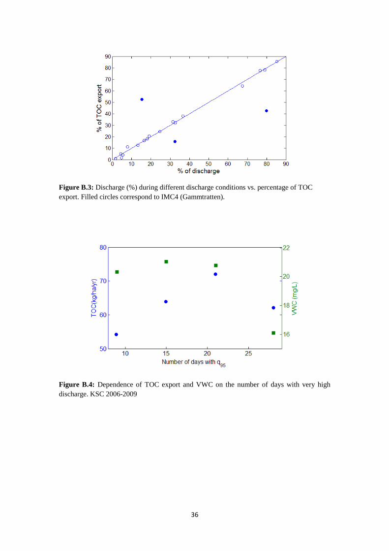
Average TOC export rates ranged from 1.1 kg/ha/yr (during low discharge conditions) to 83.1 kg/ha/yr (during high flow conditions). The VWC had a smaller range, varying from 7.5 to 43.0 mg/l (table A.5). The average LTOC had negative correlation with the percentage of forest cover and the catchment area (fig.5). TOC export varied considerably among the discharge conditions, while the VWC varied less. The slopes of both TOC and VWC vs. catchment area decreased at qhigh comparing to qlow, indicating that both export and concentration tended to become independent of the individual characteristics of each catchment (fig.6). The LTOC difference (%) between the most and least exporting catchments ranged from ~2.5% during qhigh up to ~10% during qlow (fig.B.2). For all but one catchment (IMC4) LTOC (%) vs. q (%) closely followed the 1:1 line (table A.6, fig.B.3).

12

Figure 5: TOC(kg/ha/yr) grouped according to discharge conditions, subcatchment area (a) and forest cover % (b). The whiskers are set as the closest measured value to 1.5 interquartile range. The horizontal lines denote the mean export per subcatchment, and their widths are proportional to subcatchment area and, respectively, forest cover. KSCs, 2006-2009

Figure 6: LTOC (kg/ha/yr) and VWC (mg/L) vs. catchment area (a) and percentage of forest cover (b). qlow, qmed and qhigh are plotted with solid line/ dots, dashed line/ open circles, and dotted line/stars respectively. KSCs, 2006-2009

13

In order to examine whether the change in flow patterns influences carbon export, the numbers of days per year with q95 were plotted against the annual LTOC and VWC (fig. B.4). In contrast with Krycklan, whose four years long data did not indicate any clear relationship between the above variables, for IMC there was a linearly increasing relationship (fig.7).

Figure 7: TOC export (filled circles and solid line) and VWC (open circles and dashed line) vs. number of days with extreme discharge. IMC1, 1989-2008.

The double mass curve analysis gave similar results after using daily and monthly data, with the same KSCs lying above or below the 1:1 line, as indicated on fig. 8. The slope changes were not possible to identify though when using the daily data, and also in this case the curves appeared to lie closer to the 1:1 line (fig.8b).

Figure 8: Cumulative specific TOC flux (ΣLTOC) vs. cumulative specific discharge (Σq), using monthly (a) and daily (b) data. The catchments are indicated with the corresponding figures on the legend; the thick blue line shows the 1:1 position. KSCs, 2006-2009

14

According to the analysis performed using daily data and splitting the whole time period into discharge conditions, during low flow the TOC export of all KSCs was less than can be explained by the discharge and also different from sub-catchment to sub-catchment (fig.9); during medium flow the exports were similar for all KSCs and in good agreement with the 1:1 line; during high and q95 conditions some sites lay above (with KSC3 and KSC4 being the most outstanding) and some below the 1:1 line.

Figure 9: Cumulative LTOC vs. cumulative q, based on daily data, split in four different discharge conditions. The red dashed line shows the 1:1position, while the black lines the KSCs (a) and IMCs (b). With arrows are indicated the most notable curves (see Discussion).

15

3.2.2 TOC export during different seasons KSC and IMC

The KSC seasonal exports followed closely the seasonal discharge, while the VWC followed almost the opposite trend (fig.10, table A.8). In contrast with the KSC, all but IMC4 have lower TOC export during spring compared to winter (fig.11, table A.9).

Figure 10: Seasonal average over all KSC sites TOC export and VWC

The stream in the Gårdsjön IMC dries out regularly during February and August. These drying events did not result in increased VWC during the following months (fig.11). In accordance with the flow conditions grouping, the TOC export was different from season to season and mostly discharge dependent, while the VWC values were less variable. The slopes of linear regression of TOC export and VWC vs. catchment area were almost the same across the seasons, with only spring having a smaller slope (fig. B.5), which again indicated a weaker relationship between export and catchment characteristics during high flow dominant periods.

16

Figure 11: Monthly average TOC export (kg/ha) and volume weighted concentrations for IMCs.

LCs The group of LCs consists of many rivers spread over a large area of the country, the geographic locations of which are affecting their TOC content (fig. 12). The natural logarithm of export decreased relatively consistently with increasing latitude of monitoring station, while TOC concentration had a large stepwise drop at 61.21˚N (with the exception of LC3, since Råne is not a mountain river and the catchment is forested).

Figure 12: Seasonal TOC export and concentration for different latitudes.

17

LTOC decreased with increasing catchment area as in the previous cases, but here can also be seen the separation of LC into two subgroups, the northern LC (N-LC) and the southern LC (S-LC) (fig. 13). The natural logarithm of average seasonal TOC export from S-LC showed a negative linear relationship with the natural logarithm of catchment area (R2=0.97 for spring); while N-LC were much more dispersed. Also the TOC concentration was almost independent of area in both cases but N-LCs, again with the exception of LC3, were dispersed and much smaller.

Figure 13: Average seasonal LTOC (a) and [TOC] (b) vs. catchment area. With dots and open circles are denoted the monitoring sites located north and sounth of 61˚N respectively.

All the catchments (except KSC for the subcatchments of which were assumed the same specific discharge and therefore no difference can be seen on the current plot) had increasing TOC export with increasing average discharge (fig. 14a). The S-LCs appeared to be the most sensitive to discharge increase and on average had the greatest exports per unit area. Concentration dependence on the other hand could most easily be identified for the N-LCs, while S-LC had little to negligible response (fig.14 b and d) Finally, LTOC from LCs was more strongly related to catchment area than the smaller IMCs and KSCs (fig.14 c), but generally the increasing catchment area resulted in decrease of both export and concentration for all size streams.

18

Figure 14: TOC export per unit area and concentration vs. average specific discharge and catchment area. Winter (w), spring (sp), summer (s) and autumn (a) are plotted with blue, green, red and light blue respectively.

3.2.3 TOC export per season and per discharge condition

The TOC export across KSCs varied more during low than during high discharge for all the seasons. During low and medium discharge average exports were similar during all seasons, except autumn with high export during medium discharge conditions. The largest difference among the seasonal exports was determined during high discharge (table A.10, fig.15).

19

Figure 15: TOC export (kg/ha) per season per flow condition for KSCs. The size of the circle corresponds to the catchment area.

3.3 DIC export, KSC Both downstream export and evasion of DIC had the same response to flow change (fig.16). Discharge increase could explain well the amount of DIC export increase during medium and extreme flow, while during low and high flow all the catchments deviate from the 1:1 line.

Figure 15: Cumulative LDIC (downstream export) vs. cumulative q, split in four discharge conditions. All the catchments and the 1:1 line are plotted with black curves and red dashed line respectively. KSC, 2006-2009

20

The average amount of DIC downstream export per unit area was independent of catchment area, with linear fitting p-value>0.05 (fig.17a); for evasion though (fig.17b) the stream area was important, as for small headwater streams the export per unit area is much larger (also according to Wallin et al., 2010). The DIC evasion was also dependent on stream length (fig. 18).

Figure 17: Average LDIC vs. catchment area for downstream DIC export (a) and DIC evasion (b). The p-values are given for the linear fitting of ln(LDIC) vs. ln(area). On (b) are indicated the numbers of the three subcatchments with the largest evasion.

Figure 18: LDIC (evasion) vs. stream length

21

3.4 Interseasonal dependence of TOC export

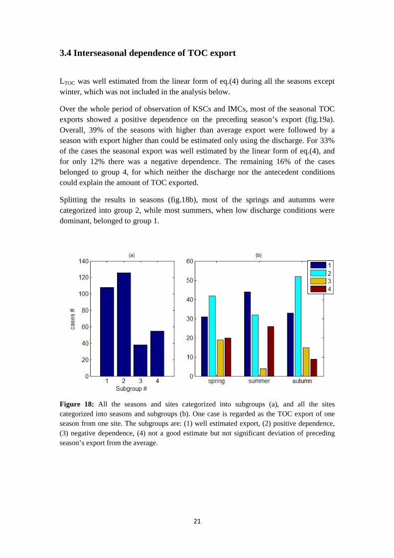
LTOC was well estimated from the linear form of eq.(4) during all the seasons except winter, which was not included in the analysis below.

Over the whole period of observation of KSCs and IMCs, most of the seasonal TOC exports showed a positive dependence on the preceding season’s export (fig.19a). Overall, 39% of the seasons with higher than average export were followed by a season with export higher than could be estimated only using the discharge. For 33% of the cases the seasonal export was well estimated by the linear form of eq.(4), and for only 12% there was a negative dependence. The remaining 16% of the cases belonged to group 4, for which neither the discharge nor the antecedent conditions could explain the amount of TOC exported.

Splitting the results in seasons (fig.18b), most of the springs and autumns were categorized into group 2, while most summers, when low discharge conditions were dominant, belonged to group 1.

Figure 18: All the seasons and sites categorized into subgroups (a), and all the sites categorized into seasons and subgroups (b). One case is regarded as the TOC export of one season from one site. The subgroups are: (1) well estimated export, (2) positive dependence, (3) negative dependence, (4) not a good estimate but not significant deviation of preceding season’s export from the average.

22

4. Discussion

The first point to be discussed is if the interpolated TOC time series was acceptable. According to the results, if there is roughly one measurement per 15 days, the interpolated export is close enough to the actual, with approximately 3.2% error. Using linear interpolation between the existing points though led to underestimation of the peak export events, and generally in smoothing the dataset. This could be one source of error, and a possible reason that the TOC export from KSCs and IMCs appeared to have fairly different responses to the discharge increase (fig.8). The cut-off of the peaks could account for the IMCs being almost identical with the 1:1 line during all except low discharge conditions.

It was chosen not to use the catchments with long term discharge trend, therefore only 24 LCs were examined. It would not have been difficult to de-trend the discharge data, in this case though the identification of a relationship between TOC export and the de-trended discharge would be misleading. It could appear for instance that the TOC export had long term variations that were not in accordance with long term discharge variations. On the other hand, de-trending TOC export data would not be possible, due to the difficulty to quantify the TOC variations resulting only from discharge variations.

The TOC export was largely dependent on discharge for all studied catchments, which is in agreement with previous studies (e.g. Hinton et al., 1998). Especially during q95 discharge conditions, TOC export was well explained from the discharge, and a close to linear relationship was seen between these variables (fig.9). The very high discharge conditions were of particular interest, as they accounted for ~30% of discharge and TOC export (for KSCs, IMC1, IMC3) while occupying only 5% of the observation period. Hence, an increase in the intensity or frequency of discharge events in a potential future climate would be expected to result in linear response of TOC export from KSCs and IMCs (fig.7).

Here must be noted though that TOC export during q95 from IMC2 and IMC4 was much smaller as compared to the other catchments (20% and 16% of the total export respectively), the TOC concentration of which were also reported not to be as much discharge dependent as the other IMCs (Winterdahl et al. 2011). For the LCs it was more difficult to identify any effect of very high discharge conditions on LTOC, because only total monthly TOC export data was available. In contrast with IMCs though, there was no significant relationship between the number of days with q95 per year and the total amount of carbon exported per year.

23

The increasing trend in TOC concentration in KSCs during the four years of study period (43% higher on 2009 than on 2006) could not be explained by long term changes in discharge, which did not show any trend and was ~7% less on 2009 than on 2006. This is in agreement with previous studies indicating an increasing trend of TOC concentration in stream and lakes of Northern Europe, including Sweden, during the last 20 years (e.g. Löfgren et al., 2010). The most supported explanation for this is that the declining of sulphur depositions and the gradually achieved less acidic environment leads to more efficient microbial activity and also to remobilization of organic carbon (e.g. Lundin et al., 2001; Oulehle et al., 2011).

Regardless of long term trend, both simple and volume weighted concentrations followed the discharge as suggested by Hinton et al. (1998) and Ågren et al. (2007): at the two KSCs with the highest percentage of wetlands (approximately 40% and 36%) the concentration followed a shortly increasing and then decreasing trend with increasing discharge, while the KSCs with higher percentage of forest cover had increasing TOC concentration with increasing discharge. This was the case for all the catchments studied, regardless their size.

The grouping of LTOC and [TOC] according to the seasons showed again that these two variables were mainly discharge driven. Also, the q – LTOC and q – [TOC] relationships was similar for all the seasons, as indicated from the fact that both export and concentration vs. discharge curves were roughly parallel across the seasons. Other parameters that could possibly influence TOC export were not taken into account, although the results would have been more accurately explained if parameters like freezing of soil in the upper layers (Haei et al., 2010), flow paths

(Dosskey and Bertsch,1994) and temperature (Winterdahl et al., 2011).

Increasing catchment area and forest cover resulted in decreasing TOC export per unit area and concentration for KSCs and IMCs, which is in agreement with previous studies (e.g. Laudon et al., 2011; Clark et al., 2010). Apart from catchment area, the LCs’ TOC exports were also dependent on the catchments’ geographical locations. The southern LCs were more TOC-rich than the northern LCs, with concentrations not deviating much from site to site and with weaker dependence on catchment area. Put together all the catchments studied (fig.14), it was possible to identify the same export/concentration – area trends for all the subgroups, but it was not easy to quantitatively describe the above relationships. Comparing all the subgroups, it was also shown that of all the catchments the LTOC of northern LCs was most sensitive to discharge increase; keeping this in mind, together with the fact that the higher latitude boreal regions will be more severely affected by the ongoing climate change (Laudon et al., 2011), it’s essential to study more extensively the northern LCs in order to best quantify the TOC cycle.

The DIC export per unit area from small head-streams was remarkably larger than from larger streams; characteristically, during the observation period, KSC5 average annual CO2 export per square meter was about 500 times larger than that of KSC15.

24

While the downstream LDIC did not vary significantly with the length of the stream, the evasion was clearly dependent on it (Wallin et al., 2010). This fact points out the need to monitor small streams in order to construct a more complete picture of the carbon cycle. Ignoring these small but important streams would lead to underestimation of CO2 input from surface waters into the atmosphere.

Regarding the interseasonal dependence of TOC exports, most of the cases studied were categorized into the ‘positive dependence’ group (38% of the cases). The positive relationship was most common during spring and autumn. Only 12 % of the cases belonged to the ‘negative dependence’ group, therefore for the discharge and catchment types examined here the cases of TOC depletion due to higher than average export were highly unlucky. During summer, when the low discharge was dominant, the export was well predicted form discharge. The fourth group included the 17% of the studied cases. For these cases the preceding season did not have too high or too low export, nevertheless the discharge was not a good estimator of the following season’s export. This seems to indicate that the perceptual accumulation and flushing model is too simple to describe the effect of antecedent conditions of the catchment. All the parameters mentioned previously to be determining TOC concentration in stream-water (e.g. soil temperature, frost history, organic matter availability) could be considered as potential causes for interseasonal TOC export dependence. An example of a catchment that could be described only by the two factors of discharge and previous season’s TOC export is IMC1. Almost every year (from 1989-2008) the stream dried out twice, around February and around August, for a duration of approximately one month (see fig.15a). On the following months there was an abrupt increase in TOC export. Possible causes for this increase might be related to the discharge condition change or also to accumulation of organic carbon in the soil during the drought, which was released afterwards. On the other hand no similarly marked increase was observed in volume weighted concentration during the following months (fig. 15b), indicating lack of negative interseasonal dependence. The same result was obtained by the method proposed here; during the 19 years long record of IMC1 only the 16% of springs and 0% of autumns following the relatively low export winters and summers indicated negative correlation.

The result from IMC1 cannot be generalized on other catchments, since there were too many unpredicted variations from case to case and the method used here was too general and simplistic. It could indicate though that for the IMC1 the event of around one month long drought is not enough to accumulate so much TOC to be detected as excess during the following month.

25

Concluding remarks

The dependence on discharge and catchment area of TOC export from streams with catchment areas varying across wide range from 2.5·10-2 to 3.4·104 km2 was found to be the same qualitatively, though it was not possible to quantify this dependence, as it varied largely among the studied catchments. Even thought TOC concentration was discharge – dependent, the long term increasing trend of concentration in all studied catchments could not be explained by any corresponding trend in discharge. The antecedent conditions effect on current TOC export was identified for 50% of the studied cases, out of which 38% suggested positive and 12% negative dependence. The existence of at least one catchment that confirmed the method used here (estimating the TOC export based only on discharge and previous season’s export) was encouraging, but this result can by no means be generalized over other catchments.

26

Cited literature Clark J.M., Bottrell S.H., Evans C.D., Monteith D.T., Bartlett R., Rose R., Newton R.J., Chapman P.J., 2010,The importance of the relationship between scale and process in understanding long-term DOC dynamics, Science of the Total Environment 408 (2010) 2768–2775 Cole J. J., Prairie Y. T., Caraco N. F., McDowell W. H., Tranvik L. J., Striegl R. G., Duarte C. M., Kortelainen P., Downing J. A., Middelburg J. J., and Melack J., 2007, Plumbing the Global Carbon Cycle: Integrating Inland Waters into the Terrestrial Carbon Budget, Ecosystems, Vol. 10, No. 1 (February, 2007), pp. 171-184 Dosskey, M. G. and Bertsch P. M., 1994. Forest sources and pathways of organic matter transport to a blackwater stream: a hydrologic approach. Biogeochemistry 24: 1 – 19 Haei M., Öquist M.G., Buffam I., Ågren A., Blomkvist P., Bishop K., Ottosson Löfvenius M., and Laudon H., 2010, Cold winter soils enhance dissolved organic carbon concentrations in soil and stream water, Geophysical Research Letters, vol. 37, L08501, doi:10.1029/2010GL042821 Kling G.W., Kipphut G.W., Miller M.C., 1991, Arctic Lakes and Streams as Gas Conduits to the Atmosphere: Implications for Tundra Carbon Budgets, Science, Vol.251 298- 301 Laudon H., Berggren M., Ågren A., Buffam I., Bishop K., Grabs T., Jansson M., and Köhler S., 2011, Patterns and Dynamics of Dissolved Organic Carbon (DOC) in Boreal, Streams: The Role of Processes, Connectivity, and Scaling; Ecosystems, doi: 10.1007/s10021-011-9452-8 Lundin L., AAstrup M., Bringmark L., Bråkenhielm S., Hultberg H., Johansson K., Kindbom K., Kvärnas H., Löfgren S., 2001, Impacts from deposition on Swedish forest ecosystems identified by integrated monitoring; Water, Air and Soil Pollution 130: 1031-1036

Löfgren S., Gustafsson J. P., Bringmark L., 2010, Decreasing DOC trends in soil solution along the hillslopes at two IM sites in southern Sweden — Geochemical modeling of organic matter solubility during acidification recovery, Science of the Total Environment 409 201–210 Hinton M.J., Schiff S.L. and English M.C., 1998, Sources and flowpaths of dissolved organic carbon during storms in two forested watersheds of the Precambrian Shield, Biogeochemistry 41: 175-197 Oulehle F., Evans C.D., Hofmeister J., Krejci R., Tahovska K., Persson T., Cudlin P. and Hruska J., 2011, Major changes in forest carbon and nitrogen cycling caused by declining sulphur deposition, Global Change Biology 17, 3115–3129, doi: 10.1111/j.1365-2486.2011.02468.x Seibert J., Grabs T., Köhler S., Laudon H., Winterdahl M., and Bishop K., 2009, Linking soil- and stream-water chemistry based on a Riparian Flow-Concentration Integration Model, Hydrol. Earth Syst. Sci., 13, 2287–2297 Schumacher B.A., April 2002, Methods for determination of total organic carbon (TOC) in soils and sediments, NCEA-C- 1282 EMASC-001

27

Visco G., Campanella L., Nobili V., 2005, Organic carbons and TOC in waters: an overview of the I nternational norm for its measurements, Microchemical Journal 79 185– 191 Wallin M., Buffam I., Öquist M., Laudon H., and Bishop K., 2010, Temporal and spatial variability of dissolved inorganic carbon in a boreal stream network: Concentrations and downstream fluxes, Journal of Geophysical Research, vol. 115, G02014, doi: 10.1029/2009JG001100 Winterdahl M., Temnerud J., Futter M.N., Löfgren S., Moldan F., Bishop K., 2011, Riparian Zone Influence on Stream Water Dissolved Organic Carbon Concentrations at the Swedish Integrated Monitoring Sites ,A Journal of the Human Environment 40(8):920-930, doi:

10.1007/s13280-011-0199-4 Öquist M.G., Wallin M., Seibert J., Bishop K., Laudon H., 2009, Dissolved Inorganic Carbon Export Across the Soil/Stream Interface and Its Fate in a Boreal Headwater Stream, Environ. Sci. Technol. 2009, 43, 7364–7369, doi: 10.1021/es900416h

Ågren A., Buffam I., Jansson M., and Laudon H., 2007, Importance of seasonality and small streams for the landscape regulation of dissolved organic carbon export, Journal of Geophysical Research, vol. 112, G03003, doi: 10.1029/2006JG000381 Ågren A., Jansson M., Ivarsson H., Bishop K. and Seibert J., 2007, Seasonal and runoff-related changes in total organic carbon concentrations in the River Öre, Northern Sweden, Aquat. Sci. 70 , 21 – 29, doi:10.1007/s00027-007-0943-9

28

Further reading Albert J. M., 2004, Hydraulic analysis and double mass curves of the Middle Rio Grande from Cochiti to San Marcial, New Mexico. Fort Collins, CO: Colorado State University. Thesis. Bishop K., Seibert J., Köhler S.and Laudon H., 2004, Resolving the Double Paradox of rapidly mobilized old water with highly variable responses in runoff chemistry, Hydrol. Process. 18, 185–189, DOI: 10.1002/hyp.5209 Bishop K., Buffam I., Erlandsson M., Fölster J., Laudon H., Seibert J. and Temnerud J., 2008, Aqua Incognita: the unknown headwaters, J., Hydrol. Process. 22, 1239–1242 Brian A. Schumacher, April 2002, Methods for the determination of total organic carbon (TOC)in soils and sediments, NCEA-C- 1282 EMASC-001 Buffam I., Laudon H., Temnerud J., Mörth C.M., and Bishop K., 2007, Landscape-scale variability of acidity and dissolved organic carbon during spring flood in a boreal stream network, Journal of Geophysical Research, vol. 112, G01022, doi:10.1029/2006JG000218 Buffam I., Laudon H., Seibert J., Mörthd C.M., Bishope K., 2008, Spatial heterogeneity of the spring flood acid pulse in a boreal stream network, Science of the Total Environment 407(2008)708–722 Butman, D. and Raymond P. A., 2011, Significant efflux of carbon dioxide from streams and rivers in the United States, Nature Geoscience, 4(12), 839-842 Eimers M. C., Buttle J., and Watmough S.A., 2008, Influence of seasonal changes in runoff and extreme events on dissolved organic carbon trends in wetland- and upland-draining streams1, Can. J. Fish. Aquat. Sci. 65: 796–808, doi:10.1139/F07-194 Grabs T., 2010, Water quality modeling based on landscape analysis: importance of riparian hydrology, Dissertations from the Department of Physical Geography and Quaternary Geology No 24 Hinton M.J., Schiff S.L. and English M.C., 1997, The significance of storms for the concentration and export of dissolved organic carbon from two Precambrian Shield catchments, Biogeochemistry 36: 67-88,

Hultberg, H., Hultengren, S., Grennfelt, P., Oskarsson, H., Kalén, C. & Pleijel, H. 2005, Air

pollution, environment and future. 30 years of research on forest, soils and water.

Gårdsjöstiftelsen and Naturcentrum AB.

Kling G.W., Kipphut G.W. & Miller M.C., 1992, The flux of CO2 and CH4 from lakes and rivers in arctic Alaska, Hydrobiologia 240: 23-36 Löfgren, S. ,2007, Integrated monitoring of the environmental status in the Swedish forest ecosystems-IM, Annual report of 2007, Department of Environmental Assessment.

Monteith D.T., Stoddard J.L., Evans C.D., de Wit H.A., Forsius M., Høgåsen T., Wilander A., Skjelkvåle B.L., Jeffries D.S., Vuorenmaa J., Keller B., Kopácek J. & Vesely J., 2007, Dissolved organic carbon trends resulting from changes in atmospheric deposition chemistry, Nature, Vol 450, doi:10.1038/nature06316

29

Payment P., M. Waite and A. Dufor, Introducing parameters for the assessment of drinking water quality (chapter 2), Assessing Microbial Safety in Drinking Water – Improving approaches and methods

Temnerud J., Seibert J., Jansson M., Bishop K., 2007,Spatial variation in discharge and concentrations of organic carbon in a catchment network of boreal streams in northern Sweden, Journal of Hydrology 342, 72– 87 Åkerblom S., Meili M., Bringmark L., Johansson K., D.B. Kleja

and Bergkvist B., 2008,Partitioning of Hg between solid and dissolved organic matter in mor layers , Water Air and Soil Pollution , Volume: 189, Issue: 1-4, Pages: 239-252, doi: 10.1007/s11270-007-9571-1

30

Appendix A Table A.1: Characteristics of KSCs site subcatchment

area size (ha) stream area (ha)

forest (%)� wetland (%)�

KSC1* 66 0.1 98.7 1.3 KSC2 13 0.02 100 0 KSC 3 2.5 10� 24 76 KSC 4 19 1.5·10� 59.6 40.4 KSC 5 95 3·10� 59 36.3 KSC 6 140 0.12 72.8 24.1 KSC 7 50 0.074 85.1 14.9 KSC 9 314 0.63 84.9 13.8 KSC 10 294 0.6 74.2 25.8 KSC 12 540 0.39 84.1 15.5 KSC 13 720 1.16 89.1 9.9 KSC 14 1285 2.9 90.4 5.1 KSC 15 1990 10.96 83.2 14 KSC 16 6700 15.35 88 8.3 a. Modified from Buffam et al., [2007] * KSC=Krycklan study catchment

Table A.2: Characteristics of IMCs

Gårdsjön (IMC1)

Aneboda (IMC2)

Kindla (IMC3)

Gammtratten (IMC4)

Catchment area (ha) 3.7 19.0 19.1 45.0 Longitude (˚) 14.90 14.50 13.18 18.13 Latitude (˚) 59.75 57.01 60.28 63.86 � �������(�)� 114-140 210-240 312-415 410-545 ������������� 90.7 96.3 91.4 92.1 ������ − ���������� �� 4.5 0 2.0 1.8 Open mire 0 0 1.3 4.3

a. Modified after Löfgren (2005)

Table A.3: IMC data available

Gårdsjön Aneboda Kindla Gammtratten Study period 01/01/89–

31/12/08 15/01/97– 31/12/08

01/01/98– 31/12/08

16/06/99– 31/12/08

Missing data - 10/04/03– 17/05/03

10/06/98-13/07/98

21/01/01-02/04/01 21/12/01-07/02/02 09/11/02-25/04/03

31

28/02/06-10/04/06

Droughts 25/06/89-28/09/89 01/10/89-15/10/89 08/06/92-2708/92 13/06/93-27/06/93 30/06/93-09/07/93 01/07/94-02/09/94 05/08/95-14/09/95 20/12/95-09/01/96 27/01/96-12/02/96 17/02/96-23/02/96 21/07/96-12/09/96 17/09/96-28/09/96 19/07/97-26/08/97 29/08/03-09/10/03 02/06/04-24/06/04 07/02/06-17/02/06 01/17/08-09/07/08 26/07/08-03/08/08

03/08/99-08/08/99

25/11/98-01/12/98 13/06/01-28/06/01

-

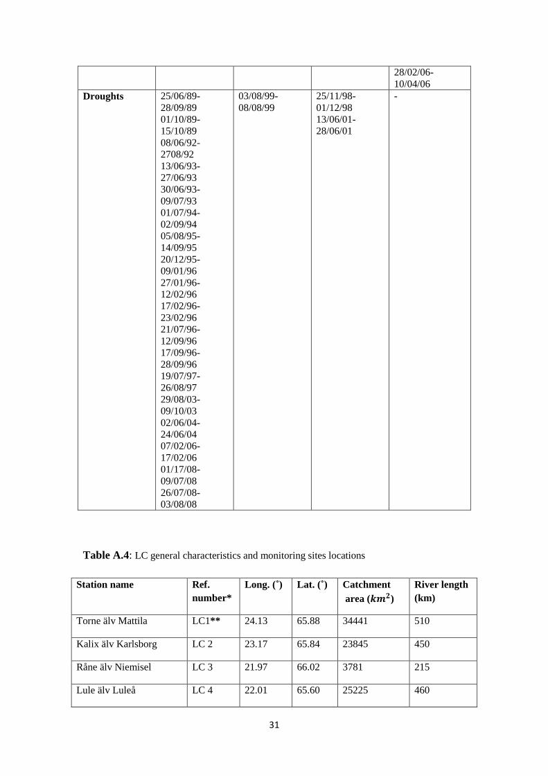
Table A.4: LC general characteristics and monitoring sites locations

Station name Ref.

number* Long. (˚) Lat. (˚) Catchment

area ( !") River length (km)

Torne älv Mattila LC1** 24.13 65.88 34441 510

Kalix älv Karlsborg LC 2 23.17 65.84 23845 450

Råne älv Niemisel LC 3 21.97 66.02 3781 215

Lule älv Luleå LC 4 22.01 65.60 25225 460

32

Pite älv Bölebyn LC 5 21.29 65.38 11285 400

Ume älv Stornorrfors LC 6 20.05 63.85 26567 465

Öre älv Torrböle LC 7 19.70 63.70 2860 240

Ångermanälven Sollefteå LC 8 17.26 63.17 30638 460

Indalsälven Bergeforsen LC 9 17.39 62.52 25767 430

Ljungan Skallböleforsen LC 10 16.96 62.36 12085 400

Delångersån Iggesund LC 11 17.09 61.63 1992 155

Ljusne Strömmar LC 12 17.08 61.21 19820 440

Gavleån Gävle LC 13 17.12 60.67 2453 130

Nyköpingsån Spånga LC 14 16.92 58.83 3589 150

Motala Ström Norrköping LC 15 16.12 58.59 1587 285

Alsterån Getebro LC 16 16.16 57.01 1333 125

Mörrumsån Mörrum LC 17 14.75 56.18 3365 185

Skivarpsån Skivarp LC 18 13.59 55.45 102 25

Råån Helsingborg LC 19 12.78 56.00 166 30

Rönneån Klippan LC 20 13.15 56.12 963 115

Nissan Halmstad LC 21 12.87 56.69 2677 200

Viskan Åsbro LC 22 12.31 57.24 2160 140

Örekilsälven Munkedal LC 23 11.69 58.46 1335 90

Enningdalsälv N.Bullaren LC 24 11.53 58.88 631 90

* This is the reference number in this project and not the real one of the station ** LC= Large Catchment

Table A.5: LTOC (kg/ha/yr) and VWC (mg/l) for different discharge conditions. KSC and IMC site LTOC (kg/ha/yr) VWC (mg/L)

qlow qmed qhigh q95 qlow qmed qhigh q95 KSC1 2.2 9.6 49.2 22.6 13.5 17.5 21.0 22.6 KSC2 2.2 8.7 47.5 22.0 13.1 15.8 20.3 22.1 KSC3 6.3 32.7 83.1 29.9 28.3 43.0 35.5 29.9

33

KSC4 5.1 19.9 67.5 23.5 31.0 36.3 28.8 23.5 KSC5 3.6 13.1 51.7 22.0 21.9 23.8 22.1 22.1 KSC6 2.3 9.9 46.4 20.6 13.7 18.1 19.8 20.6 KSC7 2.9 13.0 57.2 23.8 17.7 23.7 24.4 23.8 KSC9 1.9 8.8 43.3 19.3 12.1 16.0 18.5 19.3 KSC10 2.3 10.7 49.3 20.2 13.6 19.5 21.1 20.2 KSC12 2.1 9.8 46.6 19.8 12.6 17.8 19.9 19.9 KSC13 2.4 10.5 49.2 21.5 14.7 19.1 21.0 21.5 KSC14 1.5 6.9 35.3 14.9 8.3 11.8 14.2 14.9 KSC15 1.4 6.5 32.7 14.9 8.5 11.7 13.9 14.9 KSC16 3.3 3.3 17.8 15.2 6.4 10.4 13.7 15.2 IMC1 1.1 8.8 58.7 26.1 11.1 11.6 12.6 13.1 IMC2 7.5 16.6 43.4 13.8 29.2 21.2 19.1 20.4 IMC3 1.9 6.4 29.8 12.6 8.4 7.5 7.6 7.9 IMC4 1.5 6.3 42.6 30.7 6.7 9.2 10.6 10.6

Table A.6: The fraction of TOC exported during different discharge conditions and the corresponding discharge fraction (for Krycklan the range is given).

Table A.7: Average LTOC (kg/ha/season) and VWC (mg/l), KSC KSC: 1 2 3 4 5 6 7 9 10 12 13 14 15 16 winter LTOC 6.2 5.8 12.1 9.7 8.3 6.8 7.5 5.9 6.1 5.6 6.6 4.5 4.5 3.8

VWC 16.9 14.9 37.8 29.3 25.1 18.9 20.7 15.9 16.4 14.9 18.3 10.9 12.1 9.6 spring LTOC 26.9 25.6 36.6 29.5 28.8 25.2 27.8 22.8 23.4 22.9 24.5 18.1 17.1 17.3

VWC 20.2 19.2 27.5 22.1 21.6 18.9 20.9 17.1 17.6 17.2 18.4 12.8 12.8 12.9 summer LTOC 10.4 10.3 23.4 19.1 10.0 9.0 13.9 9.1 12.8 11.8 11.8 8.2 6.7 6.3

VWC 21.2 20.9 47.3 38.7 20.3 18.3 28.2 18.5 25.9 23.9 24.0 15.7 13.5 12.8 autumn LTOC 14.8 14.6 33.3 28.5 16.4 14.5 20.5 13.7 17.4 15.9 16.1 11.2 10.4 10.2

VWC 21.1 20.8 47.4 40.6 23.4 20.6 29.2 19.6 24.8 22.7 22.9 15.1 14.8 14.5

qlow qmed qhigh q95 KSC q (% ) 5 18 76.6 32.6

TOC (%) 3-6 15-22 73-83 25-39 IMC1 q (% ) 2 13 85 37

TOC (%) 1 13 86 38 IMC2 q (% ) 8 25 67 19

TOC (%) 11 25 64 20 IMC3 q(% ) 5 17 79 31

TOC (%) 5 17 78 33 IMC4 q (% ) 5 15 80 32

TOC (%) 2 53 43 16

34

Table A.8: Average LTOC (kg/ha/season), IMC

Table A.9: Average LTOC (kg/ha/season/discharge condition), KSC 2006-2009 season: winter spring summer autumn discharge: low med high low med high low med high low med high KSC1 0.6 1.8 4.9 0.4 1.6 24.8 0.7 1.6 8 0.5 4.1 10.3 KSC2 0.6 1.5 4.4 0.4 1.3 23.8 0.8 1.7 7.8 0.5 3.7 10.4 KSC3 2.1 4.4 10.3 1.2 4.1 31.1 2.3 4.1 16.9 1.3 9.9 22.2 KSC4 1.8 3.5 7.8 1.7 3.5 24.6 1.3 3.5 14.2 1.1 8.6 18.8 KSC5 1.4 3 6.7 0.9 2.7 25.1 1.0 1.8 7.2 0.6 4.8 11 KSC6 0.8 2.1 5.4 0.5 1.8 22.8 0.6 1.5 6.9 0.5 4 10 KSC7 0.9 2.3 5.9 0.5 2.1 25.2 1.0 2.3 10.6 0.7 5.8 14 KSC9 0.6 1.7 4.7 0.4 1.5 20.9 0.6 1.5 7 0.5 3.7 9.5 KSC10 0.6 1.8 4.8 0.4 1.7 21.2 0.8 1.9 10 0.5 4.8 12 KSC12 0.6 1.6 4.4 0.4 1.5 20.9 0.8 1.8 9.1 0.5 4.4 11.1 KSC13 0.8 2 5.3 0.4 1.8 22.1 0.8 1.8 9.1 0.5 4.3 11.3 KSC14 0.4 1.2 3.5 0.3 1.2 16.6 0.5 1.3 6.3 0.3 2.9 8 KSC15 0.4 1.2 3.7 0.3 1 15.7 0.5 1.1 5.1 0.3 2.8 7.3 KSC16 0.3 1 2.9 0.2 0.9 16.2 0.4 1 5 0.3 2.6 7.3

IMC1 IMC2 IMC3 IMC4 LTOC (kg/ha/season)

winter 20.8 18.4 11.2 3.4 spring 13.9 13.6 9.5 16.3 summer 4.9 16.4 5.9 14.7 autumn 23.6 19.8 11.8 11.6

VWC (mg/l)

winter 32.5 45.9 20.5 17.7 spring 47.5 83.4 97.3 46.9 summer 20.5 28.9 27.7 19.2 autumn 17.7 33.6 35.2 22.9

35

Appendix B

Figure B.1: Synthetic dataset of monthly average specific discharge, with increasing mean and variance. This example illustrates that if there is a trend it is not reliable to use fixed discharge limits over the whole dataset.

Figure B.2: Double mass curve ΣDOC-ΣQ for five different sites. The decreasing TOC export variation among the sites with increasing discharge is notable.

36

Figure B.3: Discharge (%) during different discharge conditions vs. percentage of TOC export. Filled circles correspond to IMC4 (Gammtratten).

Figure B.4: Dependence of TOC export and VWC on the number of days with very high discharge. KSC 2006-2009

37

Figure B.5: Volume weighted concentration and average TOC export vs. catchment area size for the four seasons, KSC 2006-2009.