Temporal and spatiotemporal coherence in

simple-cell responses: A generative model of

natural image sequences

Jarmo Hurri and Aapo Hyvärinen

Neural Networks Research Centre

Helsinki University of Technology

P.O.Box 9800, 02015 HUT, Finland

{jarmo.hurri,aapo.hyvarinen}@hut.fi

May 14, 2003

Abstract

We present a two-layer dynamic generative model of the statisticalstructure of natural image sequences. The second layer of the modelis a linear mapping from simple-cell outputs to pixel values, as inmost work on natural image statistics. The first layer models thedependencies of the activity levels (amplitudes or variances) of thesimple cells, using a multivariate autoregressive model. The secondlayer shows emergence of basis vectors that are localized, oriented andhave different scales, just like previous work. But in our new model,the first layer learns connections between the simple cells that aresimilar to complex cell pooling: connections are strong among cellswith similar preferred location, frequency and orientation. In contrastto previous work in which one of the layers needed to be fixed inadvance, the dynamic model enables us to estimate both of the layerssimultaneously from natural data.

1 Introduction

A central question in the study of sensory neural networks is how stimuli arerepresented or coded by neurons. One approach to studying the neural codeis to examine how its properties are related to the statistics of natural stimuli(Simoncelli and Olshausen, 2001). In this approach it is assumed that the

1

statistics of the natural input have affected the structure of the networks vianatural selection or during development.

In the visual system, the primary visual cortex is an area which is rel-atively well known from the point of view of neurophysiology. There is alarge amount of data on what different types of cells exist in this area, theresponses of these cells to different visual stimuli, and the connections andphysical layout of these cells (see, e.g., (Palmer, 1999)). Within the pastten years, researchers have proposed computational principles that relatethe properties of cells in this area to the statistics of natural stimuli. Themost influential of these theories have been sparse coding (Olshausen andField, 1996; Hyvärinen and Hoyer, 2001), independent component analysis(ICA) (Bell and Sejnowski, 1997; van Hateren and van der Schaaf, 1998;van Hateren and Ruderman, 1998; Hyvärinen et al., 2001b), and temporalcoherence (Földiák, 1991; Kayser et al., 2001; Wiskott and Sejnowski, 2002;Hurri and Hyvärinen, 2003). In sparse coding, the fundamental property ofthe neural code is that only a small proportion of the cells is activated by agiven stimulus. In independent component analysis, the outputs of differentcells are as independent of each other as possible. In the case of image data,these two principles are closely related (Hyvärinen et al., 2001b).

The principle of temporal coherence (Földiák, 1991; Mitchison, 1991;Stone, 1996) is based on the idea that when processing temporal input,the representation changes as little as possible over time. This principlehas been traditionally associated with complex cells (Földiák, 1991; Kayseret al., 2001; Wiskott and Sejnowski, 2002; Einhäuser et al., 2002; Berkes andWiskott, 2002), which are considered to be invariant detectors. However, ina recent paper (Hurri and Hyvärinen, 2003) we showed that a nonlinear formof temporal coherence is also related to the structure of simple-cell receptivefields. According to the results presented in (Hurri and Hyvärinen, 2003),simple-cell receptive fields are optimally temporally coherent in the sensethat the activity levels of simple cells are stable over short time intervals. Byactivity level we mean the amplitude or energy of the output of a linear filterthat models a simple cell. (The principle seems to be somewhat applicableeven in the case of non-negative, half-wave rectified cell outputs – see (Hurriand Hyvärinen, 2003) for a discussion.)

The measure of temporal activity coherence introduced in (Hurri andHyvärinen, 2003) took the sum of the temporal activity coherences of singlecells. Therefore, there was no possibility of interaction between the activitylevels of different cells. In this paper, we introduce a model which includesinter-cell activity dependencies. This is accomplished by a generative modelin which the activity levels depend on each other in an autoregressive manner.

The idea of describing natural stimuli by a generative model, and inter-

2

preting the hidden variables of this model as a neural representation, mayat first seem counterintuitive, because the stimuli are not generated by theneural network. However, if vision is considered as inverse graphics (Hintonand Ghahramani, 1997; Olshausen, 2003), the approach makes a lot of sense.A generative model can express explicitly information about the regularitiesin the stimuli as properties of hidden variables. If these regularities can beused to make inferences about the underlying real world, the visual systemwill benefit from such an internal representation of its stimuli.

The organization of this paper is as follows. In Section 2 we first give anintuitive interpretation of activity level dependencies in simple cell responsesin the case of natural stimuli. A dynamic two-layer generative model of nat-ural image sequences which captures these dependencies is then introducedin Section 3. In Section 4 we describe an algorithm for estimating the model.The validity of the algorithm is assessed using artificial (generated) data inSection 5. In Section 6, estimation of the model from natural image se-quence data is shown to yield, in one of the layers, receptive fields that havethe principal properties of simple-cell receptive fields. The other layer givesconnections between simple-cell outputs that seem to be related to both thetopographic properties of the primary visual cortex, and to the way in whichcomplex cells pool the outputs of simple cells. We conclude the paper inSection 7 by comparing our model against independent component analysis,addressing some biological considerations of the model, and discussing themerits of this work.

2 Activity-level dependencies of simple-cell-like

filters

In independent component analysis, simple cells are modeled as linear filterswhose outputs are statistically independent of each other. However, previ-ous research has already shown that the independence assumption does nothold, not even for static image input (Zetzsche and Krieger, 1999; Hyväri-nen and Hoyer, 2000; Wainwright and Simoncelli, 2000; Hyvärinen et al.,2001a; Schwartz and Simoncelli, 2001). In the case of dynamic input (im-age sequences), modeling dependencies in the resulting neural code yields anintriguing interpretation of both the structure of simple-cell receptive fieldsand the connectivity (pooling and topographic properties) of the primaryvisual cortex. In this section, we motivate such models intuitively, before theformal treatment of Section 3.

In particular, it seems that the key to modeling these dependencies is to

3

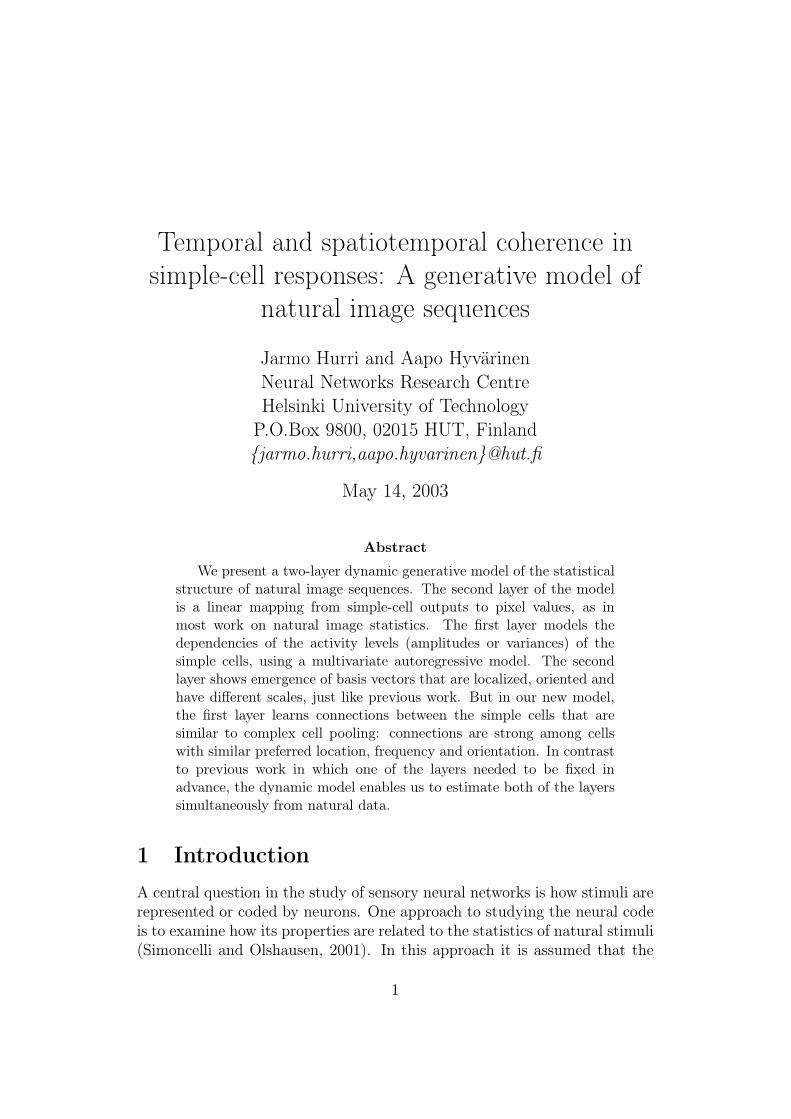
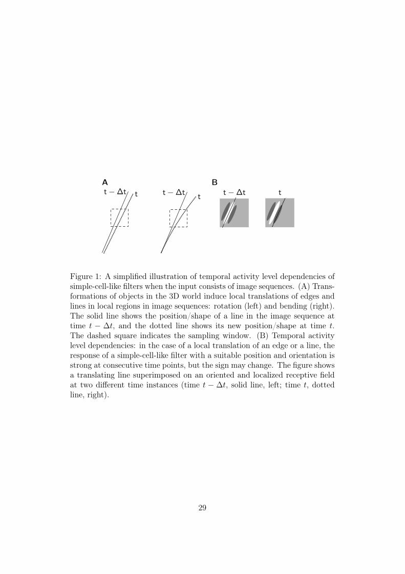
model dependencies between the activity levels – that is, amplitudes, ener-gies or variances – of the filters. We have shown in an earlier paper thatmaximization of time-correlation of output energy is an alternative to sparsecoding and independent component analysis as a computational principleunderlying simple-cell receptive field structure (Hurri and Hyvärinen, 2003).A simplified intuitive illustration of why simple-cell outputs have such strongenergy correlation over time is shown in Figure 1. Most transformations ofobjects in the 3D world result in something similar to local translations oflines and edges in image sequences. This is obvious in the case of 3D transla-tions, and is illustrated in Figure 1A for two other types of transformations:rotation and bending. In the case of a local translation, a suitably orientedsimple-cell-like filter responds strongly at consecutive time points, but thesign of the response may change (see (Hurri and Hyvärinen, 2003) for ad-ditional analysis of why the optimal filters are localized and oriented). Wecall these kinds of dependencies – dependencies over time in the outputs ofindividual filters – temporal activity level dependencies. Note that when theoutput of a filter is considered as a continuous signal, the change of signimplies that the signal reaches zero at some intermediate time point, whichcan lead to a weak measured correlation. Thus, a better model of the depen-dencies would be to consider dependencies of variances (Pham and Cardoso,2000; Valpola et al., 2003). However, for simplicity, we consider here themagnitude that is a crude approximation of the underlying variance.

[Figure 1 about here.]

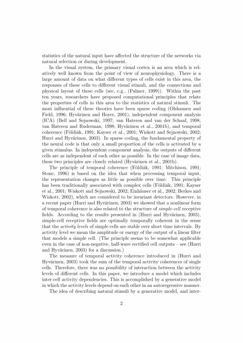
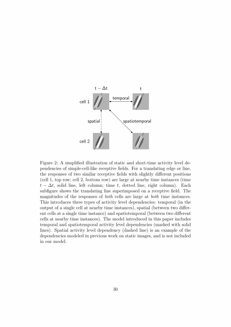
Temporal activity level dependencies, described above, are not the onlytype of activity level dependencies in a set of simple-cell-like filters. Figure 2illustrates how two different cells with similar receptive field profiles – havingthe same orientation but slightly different positions – respond at consecutivetime instances when the input is a translating line. The receptive fields areotherwise identical, except that one is a slightly translated version of theother. It can be seen that both cells are highly active at both time instances,but again, the signs of the outputs vary. This means that in addition totemporal activity dependencies (the activity of a cell is large at time t − ∆tand time t), there are two other kinds of activity level dependencies.

spatial (static) dependencies Both cells are highly active at a single timeinstance. This kind of dependency is an example of the energy depen-dencies modeled in previous research on static images (Zetzsche andKrieger, 1999; Hyvärinen and Hoyer, 2000; Wainwright and Simoncelli,2000; Hyvärinen et al., 2001a; Schwartz and Simoncelli, 2001).

4

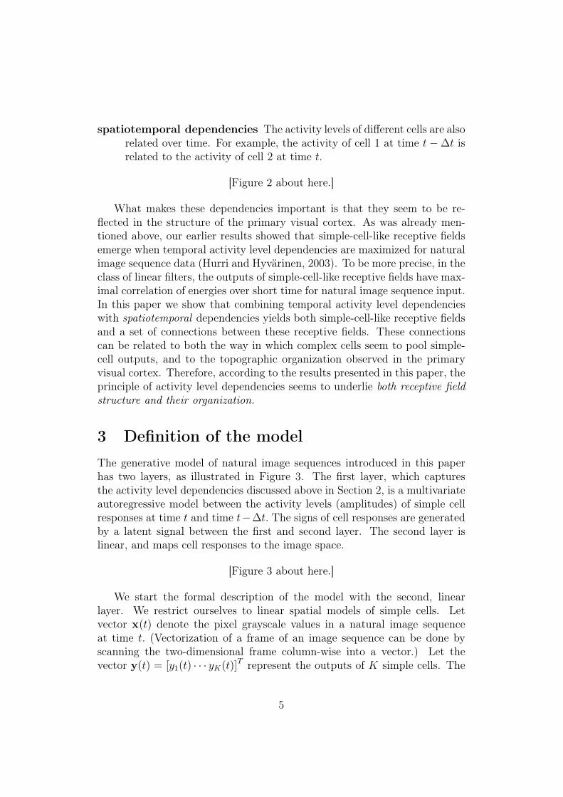
spatiotemporal dependencies The activity levels of different cells are alsorelated over time. For example, the activity of cell 1 at time t − ∆t isrelated to the activity of cell 2 at time t.

[Figure 2 about here.]

What makes these dependencies important is that they seem to be re-flected in the structure of the primary visual cortex. As was already men-tioned above, our earlier results showed that simple-cell-like receptive fieldsemerge when temporal activity level dependencies are maximized for naturalimage sequence data (Hurri and Hyvärinen, 2003). To be more precise, in theclass of linear filters, the outputs of simple-cell-like receptive fields have max-imal correlation of energies over short time for natural image sequence input.In this paper we show that combining temporal activity level dependencieswith spatiotemporal dependencies yields both simple-cell-like receptive fieldsand a set of connections between these receptive fields. These connectionscan be related to both the way in which complex cells seem to pool simple-cell outputs, and to the topographic organization observed in the primaryvisual cortex. Therefore, according to the results presented in this paper, theprinciple of activity level dependencies seems to underlie both receptive fieldstructure and their organization.

3 Definition of the model

The generative model of natural image sequences introduced in this paperhas two layers, as illustrated in Figure 3. The first layer, which capturesthe activity level dependencies discussed above in Section 2, is a multivariateautoregressive model between the activity levels (amplitudes) of simple cellresponses at time t and time t−∆t. The signs of cell responses are generatedby a latent signal between the first and second layer. The second layer islinear, and maps cell responses to the image space.

[Figure 3 about here.]

We start the formal description of the model with the second, linearlayer. We restrict ourselves to linear spatial models of simple cells. Letvector x(t) denote the pixel grayscale values in a natural image sequenceat time t. (Vectorization of a frame of an image sequence can be done byscanning the two-dimensional frame column-wise into a vector.) Let thevector y(t) = [y1(t) · · · yK(t)]T represent the outputs of K simple cells. The

5

linear generative model for x(t) is similar to the one in (Olshausen and Field,1996; Hyvärinen and Hoyer, 2001):

x(t) = Ay(t). (1)

Here A = [a1 · · · aK ] denotes a matrix which relates the image sequencegrayscale values x(t) to the outputs of simple cells y(t), so that each columnak, k = 1, ..., K, gives the feature that is coded by the corresponding simplecell. When the parameters of the model are estimated, what we obtain firstis the mapping from x(t) to y(t), denoted by

y(t) = Wx(t). (2)

The dimension of x(t) is typically larger than the dimension of y(t), sothat equation (2) is generally not invertible but an underdetermined set oflinear equations. A one-to-one correspondence between W and A can beestablished by computing the pseudoinverse solution1 A = WT (WWT )−1.

As was discussed above in Section 2, in contrast to sparse coding (Ol-shausen and Field, 1996) or independent component analysis (Hyvärinenet al., 2001b) we do not assume that the components of y(t) are independent.Instead, we assume that the activity levels (amplitudes) of the componentsof y(t) are correlated. We model these dependencies with a multivariate au-toregressive model in the first layer of our model. Let us define the activitylevels by abs (y(t)) = [|y1(t)| · · · |yK(t)|]T , and let v(t) denote a driving noisesignal (the distribution of v(t) will be discussed in more detail below). LetM denote a K ×K matrix, and let ∆t denote a time lag. Our model for theactivities is a constrained multidimensional first-order autoregressive process,defined by

abs (y(t)) = Mabs (y(t − ∆t)) + v(t), (3)

and unit energy constraints

Et

{y2

k(t)}

= 1 (4)

for k = 1, ..., K. Actually, the constraint of unit energy is not a constraintbut rather a convention. The scale of the latent variables is not well definedbecause we can arbitrarily multiply a latent variable by a constant and di-vide the corresponding column of A by the same constant without affecting

1When the solution is computed with the pseudoinverse, the solved x(t)is orthogonal to the nullspace of W, N (W) = {b ||Wb = 0} . In otherwords, that part of x(t) which would be ignored by the linear mapping inequation (2) is set to 0.

6

the model (a similar situation is found in independent component analysis).Thus, we can define the scale of the yk(t)’s as we like.

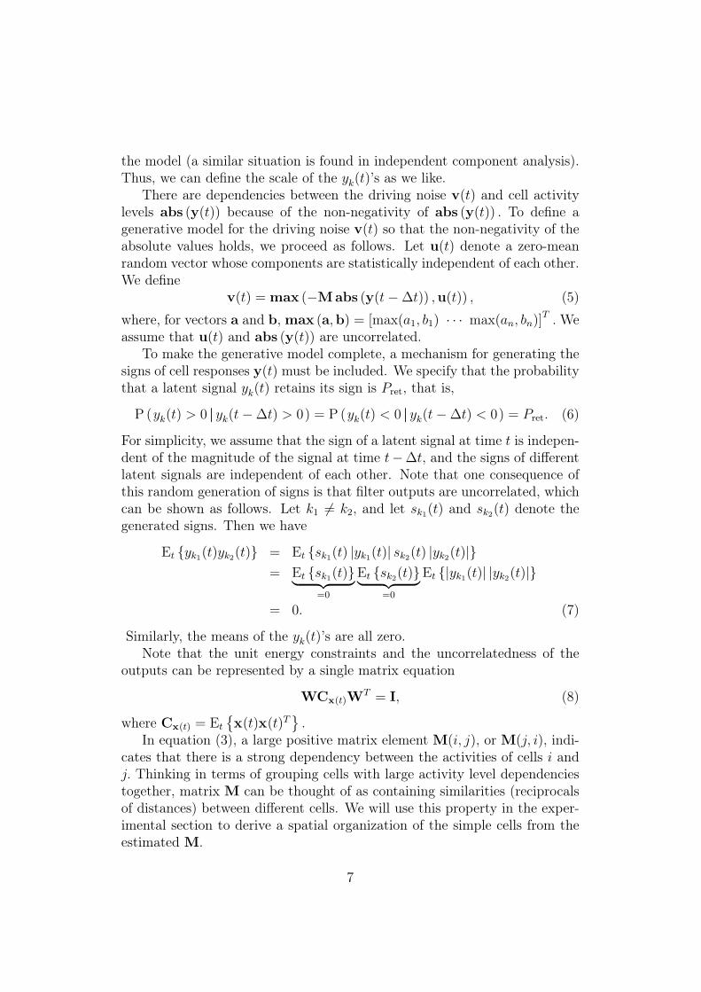
There are dependencies between the driving noise v(t) and cell activitylevels abs (y(t)) because of the non-negativity of abs (y(t)) . To define agenerative model for the driving noise v(t) so that the non-negativity of theabsolute values holds, we proceed as follows. Let u(t) denote a zero-meanrandom vector whose components are statistically independent of each other.We define

v(t) = max (−Mabs (y(t − ∆t)) ,u(t)) , (5)

where, for vectors a and b, max (a,b) = [max(a1, b1) · · · max(an, bn)]T . Weassume that u(t) and abs (y(t)) are uncorrelated.

To make the generative model complete, a mechanism for generating thesigns of cell responses y(t) must be included. We specify that the probabilitythat a latent signal yk(t) retains its sign is Pret, that is,

P (yk(t) > 0 || yk(t − ∆t) > 0) = P (yk(t) < 0 || yk(t − ∆t) < 0) = Pret. (6)

For simplicity, we assume that the sign of a latent signal at time t is indepen-dent of the magnitude of the signal at time t−∆t, and the signs of differentlatent signals are independent of each other. Note that one consequence ofthis random generation of signs is that filter outputs are uncorrelated, whichcan be shown as follows. Let k1 6= k2, and let sk1

(t) and sk2(t) denote the

generated signs. Then we have

Et {yk1(t)yk2

(t)} = Et {sk1(t) |yk1

(t)| sk2(t) |yk2

(t)|}

= Et {sk1(t)}︸ ︷︷ ︸

=0

Et {sk2(t)}︸ ︷︷ ︸

=0

Et {|yk1(t)| |yk2

(t)|}

= 0. (7)

Similarly, the means of the yk(t)’s are all zero.Note that the unit energy constraints and the uncorrelatedness of the

outputs can be represented by a single matrix equation

WCx(t)WT = I, (8)

where Cx(t) = Et

{x(t)x(t)T

}.

In equation (3), a large positive matrix element M(i, j), or M(j, i), indi-cates that there is a strong dependency between the activities of cells i andj. Thinking in terms of grouping cells with large activity level dependenciestogether, matrix M can be thought of as containing similarities (reciprocalsof distances) between different cells. We will use this property in the exper-imental section to derive a spatial organization of the simple cells from theestimated M.

7

One interpretation of the driving noise v(t) is closely related to this ideaof grouping cells with strong interdependencies together: v(t) can be consid-ered as coding for higher-order features in the dynamic data. Consider thecase in which a component of v(t), say vk(t), takes a high positive value attime t. Then the corresponding component of y(t) – that is, yk(t) – wouldalso become highly active at time t. Because of the dynamic properties ofthe autoregressive model, during consecutive time instances the activity ofyk(t) would spread to those components of y(t) for which the correspondingelements of M are large. Therefore, a large value in vk(t) codes for the ac-tivation of such a group of units with strong dependencies. In other words,vk(t) signals the occurrence of a higher-order feature that is common for thisgroup. We will see below in Section 6.2 how this interpretation relates v(t)to complex cells.

4 Estimation of the model

To estimate the model defined above we need to estimate both M and W

(the pseudoinverse of A). In this section we first show how to estimateM, given W. Then we describe an objective function which can be used toestimate W, given M. Each iteration of the estimation algorithm consistsof two steps. During the first step M is updated, and W is kept constant;during the second step these roles are reversed.

First, regarding the estimation of M, consider a situation in which W

has been fixed. It is shown in Appendix A that M can be estimated by usingan approximative method of moments. The estimate is given by

M ≈ βEt

{(abs (y(t)) − Et {abs (y(t))})

× (abs (y(t − ∆t)) − Et {abs (y(t))})T

}

× Et

{(abs (y(t)) − Et {abs (y(t))})

× (abs (y(t)) − Et {abs (y(t))})T

}−1

,

(9)

where β > 1. We will return to the role of the scalar multiplier β below.The estimation of W is more complicated. A rigorous derivation of an

objective function based on well-known estimation principles is very difficult,because the statistics involved are non-Gaussian, and the processes have dif-ficult interdependencies. Therefore, instead of deriving an objective function

8

from first principles, we derived an objective function heuristically startingfrom the least squares estimate (see Appendix B), and verified through sim-ulations that the objective function is capable of estimating the two-layermodel. The objective function is a weighted sum of the covariances of filteroutput amplitudes at times t − ∆t and t, defined by

f(W,M) =K∑

i=1

K∑

j=1

M(i, j) cov {|yi(t)| , |yj(t − ∆t)|} , (10)

which can also be expressed as

f(W,M) = Et

{(abs (y(t)) − Et {abs (y(t))})T

M

× (abs (y(t − ∆t)) − Et {abs (y(t))})

}.

(11)

(The function f depends on W through the relationship (2).) The estimationof W is thus accomplished by maximizing this objective function

W = arg maxW

f(W, M). (12)

Optimization of the objective function f over W under constraint (8) uses agradient projection approach (Hurri and Hyvärinen, 2003). The initial valueof W is selected randomly.

When the model is estimated from natural image sequence data, the valueof the scalar multiplier β in (9) can not be estimated. However, first notethat this multiplier has a constant linear effect in objective function (10).This means that the value of β does not affect the optima of (10), so thecorrect value of β is not needed to estimate W. Second, multiplier β onlyscales the elements of M with a constant value. This rescaling does not affectthe ratios of the elements, or their ordering. In addition, as was discussedabove, matrix M can be thought of as containing similarity measurementsbetween different cells. The multiplication of M with a positive scalar doesnot modify the information contained in the measurements when an intervalmeasurement scale (Borg and Groenen, 1997) is used. We will see below inSection 6.2 that in our case the interval scale is a natural measurement scalefor the measurement distances in M. Therefore, in the estimation we just setβ = 1.

Note, however, that in the validation of the estimation method this pos-sible rescaling of M must be taken into account, because we want to measurethe convergence of the algorithm quantitatively. This will be considered indetail below.

9

5 Experiments with artificial data

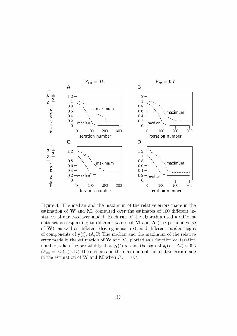
Before applying the estimation method to natural data, we verified its validityusing artificial data. We first generated 100 different matrices M and A, andused these to generate data which followed our model. The dimension of thedata was K = 10, so both M and A were 10 × 10 matrices. Input noiseu(t) was Gaussian white noise. In generating the data, care must be takenso that the the constraints are fulfilled, and that the resulting autoregressivemodel is stable. Details on how this can be done are given in Appendix C.1.

After data generation we ran our estimation algorithm 100 times, oncefor each of the data sets, to obtain estimates M and W (estimate of thepseudoinverse of A) of all the original matrices. Because of the insensitivityof the objective function (10) to a different ordering of the components of y(t),which is similar to the case of independent component analysis (Hyvärinenet al., 2001b), care had to be taken to compensate for a possible permutation;details on how this was done are described in Appendix C.2.

After compensating for the possible permutation, the effect of the un-known scalar multiplier β in equation (9) had to be accounted for. In theestimation process above we just set β = 1, because in the case of naturalimage sequence data this coefficient can be discarded as was discussed inSection 4 above. Here, however, the convergence of the algorithm is exam-ined quantitatively, so this multiplier has to be accounted for to get an exactperformance measure. This was done by using equation (9) to estimate β by

β =‖M‖F∥∥∥M

∥∥∥F

(13)

(remember that estimate M is obtained by setting β = 1 in equation (9)).Here ‖·‖F denotes the Frobenius norm, that is, ‖M‖2

F =∑

i

∑j(M(i, j))2.

To analyze the convergence of the algorithm, we examined how the rela-tive estimation errors

(∥∥M−M∥∥

F

)/ ‖M‖F and

(∥∥W−W∥∥

F

)/ ‖W‖F change

as a function of number of iterations. Figure 4 shows the resulting plots ofthe relative errors. The plots show the median and the maximum of theerrors of the estimates of M and W, computed over the whole set of 100runs. The median and maximum are plotted as a function of iteration num-ber. Two different values of Pret (see Figure 3 and equation (6)) were used intwo different sets of experiments. The results for Pret = 0.5, correspondingto perfectly temporally decorrelated data, are shown in Figures 4A and C.We also estimated the value of Pret from results obtained from natural im-age sequences, where a softer form of temporal decorrelation was used (seeSection 6). Figures 4B and D show the results obtained when the data is

10

generated using the estimated value Pret = 0.7. These results show that theestimation method is not sensitive to small variations in Pret.

[Figure 4 about here.]

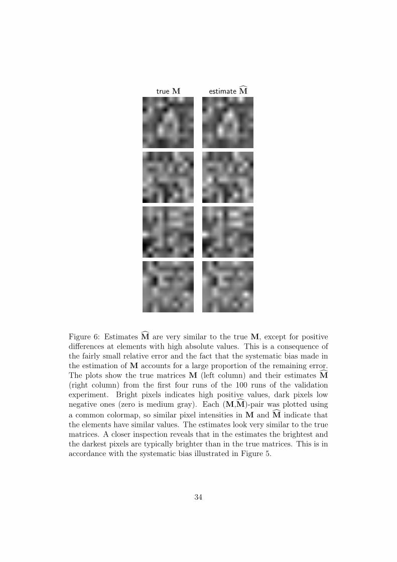
As we can see, the estimate of W converges fairly reliably to the truevalue. As for the estimation of M, the scalar multiplier β estimated as inequation (13) was consistently greater than 1, as predicted in Appendix A.The relative error of the estimate of M decreases considerably in the esti-mation, but the final estimate is not as good as in the case of W. This isprobably due to the approximation made in its estimation (see Appendix A).However, a large part of the error is caused by a simple bias in the estimate,and this bias does not seem to be critical in our analysis of the results. Thenature of the bias can be seen in Figure 5, which shows a scatter plot of thetrue elements of the 100 matrices M vs. their estimates. We can see thatthe bias is largely a nonlinear element-wise relationship between the truevalue of an element of M and its estimate. This nonlinear relationship is amonotonic convex function, characterized by larger positive deviations fromthe true value when the absolute value of the element of M is large. Remem-bering that the Frobenius norm – which is used to measure the relative error– emphasizes large errors, we can see that a large part of the relative errorresults from this bias.

[Figure 5 about here.]

In the analysis of results with real data we are mostly interested in themagnitudes of the elements of M with respect to other elements of the samematrix. These relationships are preserved by a smooth monotonic mappingof the elements of M, like the simple bias described above. In Figure 6 wehave plotted four first matrices M from the set of 100 matrices, along withtheir estimates M. Although there are some differences in some individualelements of the matrices, especially in elements with large absolute values,the structures of the true matrices and their estimates look very much alike.This is because the relative values of the elements with respect to the valuesof the other elements are similar.

[Figure 6 about here.]

11

6 Experiments with natural image sequences

6.1 Data collection and preprocessing

The data and preprocessing used in the experiments were very similar tothose in (Hurri and Hyvärinen, 2003), so we will describe them only shortlyhere, and refer the reader to (Hurri and Hyvärinen, 2003) for details.

The natural image sequences used in data collection consisted of 129image sequences, which were a subset of natural image sequences used in(van Hateren and Ruderman, 1998). The sampling rate in these sequenceswas 25 Hz. Initially 200,000 image sequences with a duration of 440 ms, andspatial size 16 × 16 pixels, were sampled from these sequences. The fairlylong duration of these initial samples was necessary because of the temporalfiltering used in preprocessing,

The preprocessing consisted of four steps: temporal decorrelation, sub-traction of local mean, normalization, and dimensionality reduction (seeSection 7.1 for an experiment in which neither temporal decorrelation nornormalization was performed). Temporal decorrelation enhances temporalchanges in the data, and differentiates our results from those obtained withstatic images (Hurri and Hyvärinen, 2003). It can also be motivated as amodel of temporal processing at the lateral geniculate nucleus (Dong andAtick, 1995). Temporal decorrelation was performed with a temporal fil-ter of length 400 ms. The length of the resulting sequences, which was alsothe time delay ∆t in our experiment, was 40 ms. That is, each preprocessedsequence consisted of two 16 × 16 frames separated by ∆t = 40 ms. Aftertemporal decorrelation, the spatial local mean (spatial DC component) wassubtracted from each of the 400,000 frames, and the frames were normalizedto unit norm. This normalization can be considered as a form of contrastgain control (Carandini et al., 1997; Heeger, 1992). Finally, to reduce theeffect of noise and aliasing artifacts (van Hateren and van der Schaaf, 1998),the dimensionality of the data was reduced to 160 using principal componentanalysis (Hyvärinen et al., 2001b).

6.2 Results

The estimation algorithm described in Section 4 was applied to the prepro-cessed natural image sequence data to obtain estimates for M and A. Figure 7shows the resulting basis vectors – that is, columns of A. As can be seen,the resulting basis vectors are localized, oriented, and have multiple scales.These are the most important defining criteria of simple-cell receptive fields(Palmer, 1999). These qualitative features are also characteristic of results

12

obtained with independent component analysis or sparse coding (Olshausenand Field, 1996; van Hateren and van der Schaaf, 1998) and purely temporalactivity coherence (Hurri and Hyvärinen, 2003). This suggests that, as faras receptive field structure is concerned, these methods are rather similar toeach other in that receptive fields with similar qualitative properties emergewhen the methods are applied to natural visual stimuli.

[Figure 7 about here.]

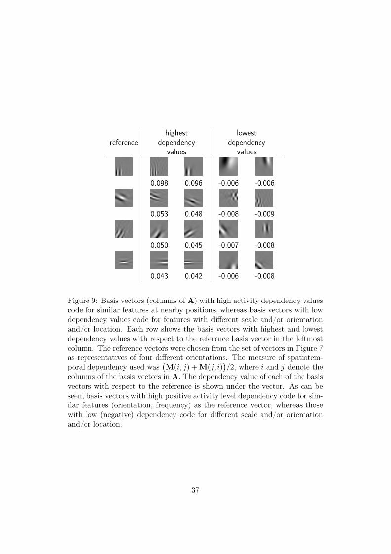
The estimated matrix M captures the temporal and spatiotemporal ac-tivity level dependencies between the basis vectors shown in Figure 7. Thediagonal elements of the estimated M were relatively large, ranging from 0.31to 0.74 with a mean of 0.44, indicating that for all the basis vectors, activitylevels at time t − ∆t and time t have considerable correlation. This is inconcordance with the results in (Hurri and Hyvärinen, 2003). A histogramof the non-diagonal elements of M, which contain the information about spa-tiotemporal dependencies between the basis vectors, is shown in Figure 8. Inorder to examine these dependencies more closely, we first plotted the basisvectors with the highest and lowest activity level dependency values for a setof representative reference vectors. The results, shown in Figure 9, suggestthat basis vectors with high positive activity level dependencies code for sim-ilar features at nearby positions, whereas basis vectors with low (negative)dependencies code for features with different scale and/or orientation and/orlocation.

[Figure 8 about here.]

[Figure 9 about here.]

To visualize the spatiotemporal dependencies of all of the basis vectors,we used the interpretation of M as a similarity matrix (see Section 3). MatrixM was first converted to a non-negative similarity matrix Ms by subtractingmini,j M(i, j) from the elements of M, and by setting the diagonal elementsto value 1. Multidimensional scaling was then applied to Ms by interpretingthe values 1 − Ms(i, j) and 1 − Ms(j, i) as distances (reciprocals of simi-larities) between cells i and j. The objective of multidimensional scaling isto map the points in a (high-dimensional) space to a two-dimensional space(a plane) so that the distances between the points in the original space arepreserved as well as possible on the plane. A central concept in the applica-tion of multidimensional scaling to a particular problem is the measurementscale (Borg and Groenen, 1997; SAS/STAT, 2000), which is a mathemat-ical description of the type of information contained in the measurements

13

of proximity. We applied multidimensional scaling to our data so that theinterval measurement scale (Borg and Groenen, 1997; SAS/STAT, 2000) wasassumed. Informally, use of the interval measurement scale means that rel-ative sizes of differences between measurements are meaningful, but there isno absolute zero. This makes sense in our case, because firstly, the differencesbetween the elements of Ms should tell us something about the differencesof strengths of spatiotemporal dependencies, and secondly, we do not knowthe maximum possible spatiotemporal dependency in natural image sequencedata (the absolute zero).

The resulting spatial layout produced by the multidimensional scalingprocedure is shown in Figure 10. Because some of the points in the pla-nar representation were very close to each other, some small distances werestretched (some of the tightest clusters were magnified) in order to be ableto show the basis vectors in a reasonable scale without overlap between thebasis patches. As in Figure 9, we can see that those basis vectors whichare very close to each other seem to be mostly coding for similarly orientedfeatures with the same frequencies at nearby spatial positions. This kind ofgrouping is characteristic of pooling of simple cell outputs at complex celllevel, as well as of the topographic organization of the visual cortex (Palmer,1999). Note that this grouping effect is not a result of the magnificationof the tightest clusters described above; in fact, the magnification reducesthe effect. In addition to the local topography described above, some globaltopography also emerges in the results: those basis vectors which code forhorizontal features are on the left in Figure 10, while those that code forvertical features are on the right.

[Figure 10 about here.]

When examining the preferred orientations of the basis vectors in Fig-ure 10, we can see that there are more vectors that prefer horizontal or verti-cal orientations than those that prefer oblique orientations. A similar imbal-ance has been observed in the visual cortex, in the number of cells preferringoblique orientations vs. the number of cells preferring horizontal/vertical ori-entations (see, e.g., (Li et al., in press)). This imbalance is thought to underliethe oblique effect, the fact that in psychophysical tests vertical and horizontalorientations are discriminated better than oblique ones. Our results suggestthat there may be a connection between the oblique effect and the statisticsof natural stimuli. We suspect that these results emerge from natural imagesequences because horizontal and vertical lines and edges are prevalent whennatural scenes are examined in an upright position, but further research isneeded to verify this.

14

It should also be noted that in Figure 10, in some cases oblique basis vec-tors whose preferred directions are orthogonal to each other are located closeto each other in the spatial layout. Note that this is not the case in Figure 9,where we can see that also in case of an oblique preferred direction, the filterswith highest dependencies have a similar orientation. Therefore, this effectdoes not seem to be a property of the extracted dependencies (matrix M);it is more likely due to distortions caused by the multidimensional scalingprocedure that forces the points to lie in a plane.

To summarize the results presented in this section, the estimation of ourtwo-layer model from natural image sequences yields, firstly, simple-cell-likereceptive fields (Figure 7), and secondly, grouping similar to the poolingof simple cell outputs and local topographic organization in the primaryvisual cortex (Figures 9 and 10). The receptive fields emerge in the secondlayer (matrix A), and cell output grouping emerges in the first layer (matrixM). Both of these layers emerge simultaneously during the estimation of themodel. This is a significant improvement on earlier statistical models of earlyvision (Hyvärinen and Hoyer, 2000; Hyvärinen and Hoyer, 2001; Wainwrightand Simoncelli, 2000), because no a priori fixing of either of these layers isneeded.

We mentioned in Section 3 that the driving noise process v(t) can codefor the occurrence of higher-order features by signalling the activation of agroup of units with strong dependencies. Statistically, a large positive valueof an element of v(t) tends to indicate the activation of such a group fora certain period of time. From Figures 9 and 10 we can now see what thehigher-order features coded by v(t) would be: short contours with a certainorientation and scale, differing in their phase and spatial position. This kindof learning of invariant features – invariant to the phase and position of anedge or line in this case – was originally associated with temporal coherenceby Földiák in his theoretical work and simulations (Földiák, 1991). In themammalian visual system, complex cells are traditionally considered to beinvariant to phase. The driving noise signal v(t) thus gives the values ofhigher-order features that could be related to complex cells.

7 Discussion

7.1 Multivariate AR model estimation vs. independent

component analysis

What happens if we try to estimate the second (linear) layer of the modelwith standard independent component analysis? Under what conditions are

15

the results different, and how? Intuitively it would seem that independentcomponent analysis would not be applicable if the activity level dependenciesbetween different components of y(t) are sufficiently strong. The strengthof these dependencies is governed by matrix M. To examine this closer wemade two experiments, one with simulated data and the other with naturalimage sequence data.

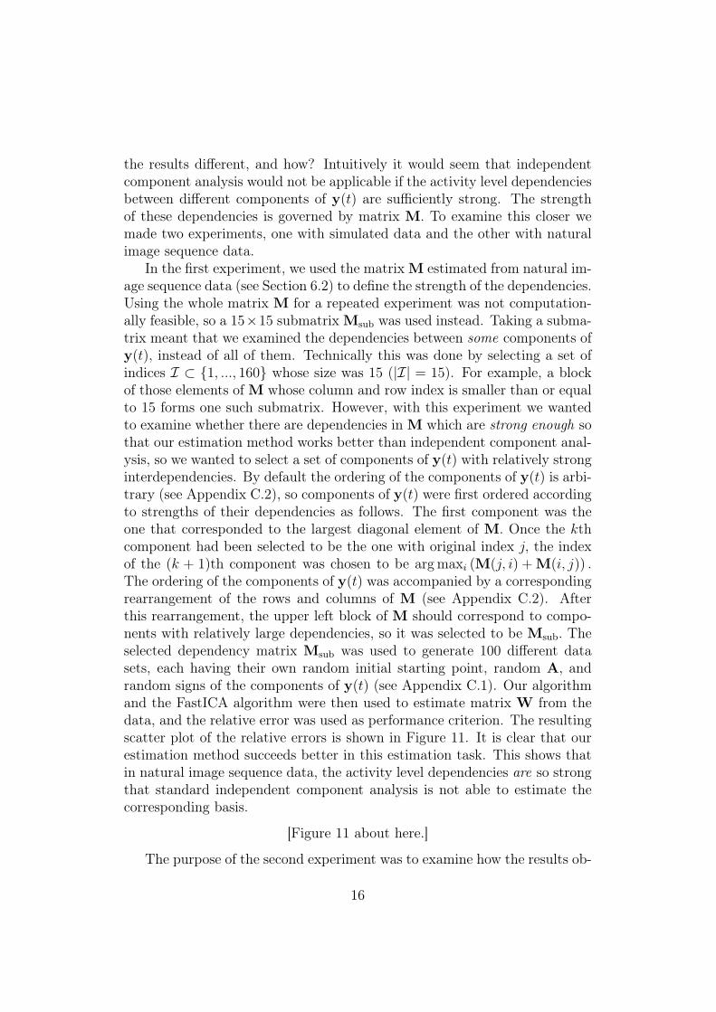
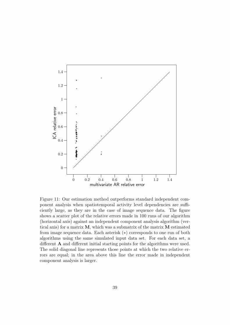
In the first experiment, we used the matrix M estimated from natural im-age sequence data (see Section 6.2) to define the strength of the dependencies.Using the whole matrix M for a repeated experiment was not computation-ally feasible, so a 15×15 submatrix Msub was used instead. Taking a subma-trix meant that we examined the dependencies between some components ofy(t), instead of all of them. Technically this was done by selecting a set ofindices I ⊂ {1, ..., 160} whose size was 15 (|I| = 15). For example, a blockof those elements of M whose column and row index is smaller than or equalto 15 forms one such submatrix. However, with this experiment we wantedto examine whether there are dependencies in M which are strong enough sothat our estimation method works better than independent component anal-ysis, so we wanted to select a set of components of y(t) with relatively stronginterdependencies. By default the ordering of the components of y(t) is arbi-trary (see Appendix C.2), so components of y(t) were first ordered accordingto strengths of their dependencies as follows. The first component was theone that corresponded to the largest diagonal element of M. Once the kthcomponent had been selected to be the one with original index j, the indexof the (k + 1)th component was chosen to be arg maxi (M(j, i) + M(i, j)) .The ordering of the components of y(t) was accompanied by a correspondingrearrangement of the rows and columns of M (see Appendix C.2). Afterthis rearrangement, the upper left block of M should correspond to compo-nents with relatively large dependencies, so it was selected to be Msub. Theselected dependency matrix Msub was used to generate 100 different datasets, each having their own random initial starting point, random A, andrandom signs of the components of y(t) (see Appendix C.1). Our algorithmand the FastICA algorithm were then used to estimate matrix W from thedata, and the relative error was used as performance criterion. The resultingscatter plot of the relative errors is shown in Figure 11. It is clear that ourestimation method succeeds better in this estimation task. This shows thatin natural image sequence data, the activity level dependencies are so strongthat standard independent component analysis is not able to estimate thecorresponding basis.

[Figure 11 about here.]

The purpose of the second experiment was to examine how the results ob-

16

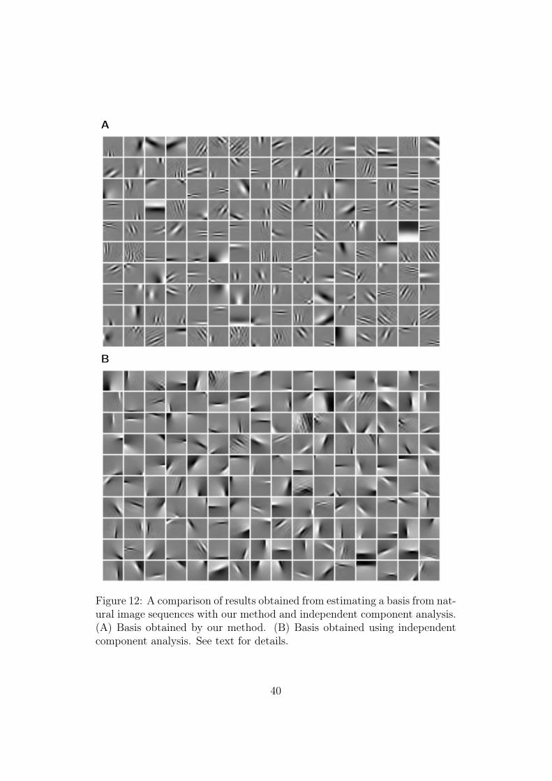
tained from natural image sequence data differ for the two methods. To makethe comparison possible, we modified the preprocessing used above (see Sec-tion 6.1) so that no temporal preprocessing or normalization was performed– that is, only the local mean was subtracted. No temporal decorrelation wasdone because it is not meaningful in the case of static independent componentanalysis, and in order for the results of the two methods to be comparablethe same data has to be used. It seems that normalization is only neces-sary as a preprocessing step when temporal decorrelation is done (probablybecause of the very large temporal changes that temporal decorrelation in-troduces into the data), so it was also left out. This experiment also servedas a control experiment to show that the qualitative properties of our originalresults (see Figure 7) were not a consequence of temporal preprocessing ornormalization. The results of both methods – our algorithm and independentcomponent analysis – are shown in Figure 12. The results are qualitativelysimilar in that in both cases the resulting filters are oriented, localized andbandpass. However, some differences can also be seen. First, the number ofsubregions (dark or light regions in the receptive fields) seems to be smallerin the ICA results. Second, most of the ICA basis vectors include a smallglobal step-like grayscale change. Thus, the difference between ICA and ourpresent algorithm can also be seen in the case of experiments on real data.

[Figure 12 about here.]

7.2 Biological considerations: underlying mechanisms,

and nonnegative simple-cell models

The theory and simulations presented in this paper model the relationshipbetween the properties of the primary visual cortex and statistics of naturalimage sequences. The underlying assumption is that the visual system hasspecialized to account for the properties of typical stimuli. In terms of bio-logical mechanisms, such specialization could be genetic, or could take placeduring development. Our model is not intended to specify at all how or whensuch specialization would take place. It only models the resulting relation-ships between an organism and its environment, not the dynamic interactionof these two, nor the role of development vs. genetic instructions.

In computational neuroscience, linear filters are typically applied as mod-els of rate coding in simple cells (Olshausen and Field, 1996; Bell and Se-jnowski, 1997; van Hateren and van der Schaaf, 1998). In reality, however,the firing rate of a cell can only be positive. This can be modeled, for exam-ple, with half-wave rectification (Heeger, 1992), in which the negative outputvalues of a linear filter are squashed to zero in the actual cell output, and

17

each output unit consists of two cells with otherwise identical receptive fieldsexcept for reversed polarities (see, e.g., (Hurri and Hyvärinen, 2003)). Theinterpretation of our model in this case is that two cell pairs, each pair con-sisting of two cells with reversed polarities, have activity level dependencies.Concerning the results obtained from natural image sequences, consider re-placing each receptive field in Figure 10 with a corresponding two-cell unit.The most important qualitative observations made from the results in Fig-ure 10 were that the receptive fields are oriented, localized and multiscale,and that connections implied by elements of matrix M are strongest betweencells with similar orientation and scale and nearby location. Replacing eachreceptive field by the corresponding two-cell unit does not change these ob-servations. The previous discussion suggests that use of a basic nonnegativesimple-cell model (half-wave rectification) should not change the qualitativenature of our results obtained from natural image sequences. However, itmust be noted that in the case of purely temporal activity level dependen-cies (horizontal direction in Figure 2), our earlier results suggest that suchdependencies are present even for individual half-wave rectified simple-cellmodels, not only for cell pairs (Hurri and Hyvärinen, 2003). Therefore, addi-tional model development and experimentation is needed before the resultsof this paper can be generalized to nonnegative cell models.

7.3 Conclusions and related work

There are two main contributions in this paper. First, to our knowledge,the generative model presented here is the first attempt to model the visualsystem using a two-layer generative model of natural image sequences. Amulti-layered description of the stimuli is important because it enables us tocapture dependencies within the different layers of sensory processing. In amulti-layered model, the processing in higher layers has an influence on theoptimality of features on the lower level and vice versa; thus joint modeling oflower and higher layer features is the only way to find out what the optimalfeatures and processing methods are. In our case, the results suggest thatsimple-cell outputs have temporal and spatiotemporal activity level depen-dencies, and that cells at the next level of processing (complex cells) poolsimple-cell outputs so that cells with high activity level dependencies arepooled together. This can provide important cues as to how different layersin the visual pathway are connected. (For on-going work on application ofanother multi-layer model of image sequences for segmentation see (Felderhofet al., 2002).)

The results obtained from natural image sequence data also suggest thatspatiotemporal activity level dependencies could also be reflected in the to-

18

pography of the primary visual cortex – that is, cells with high spatiotemporalactivity level dependencies seem to be physically located close to each otherwithin the cortex. This complements earlier research on how simultaneousactivity dependency (see Figure 2) is reflected in the organization of thecortex in a similar manner. The outputs of related wavelet filters with un-correlated outputs exhibit a similar dependency in natural images (Zetzscheand Krieger, 1999; Wainwright and Simoncelli, 2000; Schwartz and Simon-celli, 2001): the conditional variance of the output of one filter is larger whenthe output of the other filter has a large amplitude. In a more generative-model setting, dependencies between simultaneous activity levels of simplecells have been used in modeling complex cells and topography (Hyvärinenand Hoyer, 2000; Hyvärinen and Hoyer, 2001). In these models, the second(pooling) layer was fixed and only the first layer was estimated. When theseearlier results on simultaneous activity dependencies are combined with ourresults on temporal dependencies, it seems possible that “activity bubbles”(Hyvärinen et al., in press), activations of simple cells which are contiguousboth in space and time, appear on the cortical surface when a stimulus withappropriate characteristics (orientation, scale) is present in the visual field.This is an intriguing characterization of the neural code at the simple celllevel, the implications of which are a subject of future research.

Second, this paper also makes a rather different contribution, describ-ing a general-purpose two-layer model that is a generalization of the basicgenerative models used in blind source separation. The generative model de-scribed in this paper employs nonlinearities and interdependencies, resultingin a model which is difficult to solve using well-known estimation principles.Therefore, when developing the estimation algorithm, we had to resort to ap-proximation and heuristics. However, as we have shown above, the resultingalgorithm can estimate fairly well the unknown parameters from data whichfollows our model. On the average, matrix A can be estimated with verygood accuracy. Matrix M can also be recovered up to a fairly small rela-tive error, and a systematic bias which is irrelevant for most purposes. Thisgenerative model could be applied to many of those applications in whichblind source separation algorithms have been successful, such as brain imag-ing data analysis (Hyvärinen et al., 2001b). Further work on this problemcan be found in (Hyvärinen and Hurri, submitted).

Research related to the results presented here can also be found in pre-vious research on unsupervised learning and econometrics. In blind sourceseparation, Bayesian methods have been used to extract sources with non-linear dynamics and nonlinear mapping from state space to observations(Valpola and Karhunen, 2002; Valpola et al., 2003). A related study can alsobe found in (Charles et al., 2002), where it was shown that in the case of

19

simulated data (vertically or horizontally moving lines), temporally relatedfeatures can be forced to be coded in the same areas in a noisy nonlinear prin-cipal component analysis network. This was done by introducing spatiallyseparate noisy areas in a network having time-delayed lateral connectionsbetween neighboring cells – both the separate noisy areas and the lateralconnections introduce the pooling property a priori into the network. Ineconometrics, autoregressive conditional heteroskedasticity (ARCH) models(e.g., (Bera and Higgins, 1993)) are used to model econometric time series inwhich variance changes over time, and is highly correlated over time, therebyexhibiting temporal coherence of high activity. Multivariate ARCH modelscan be used to model cases where the variances of different time series havedependencies.

To conclude, we have described a two-layer dynamic generative model ofimage sequences, and an algorithm for estimating the model from sampledata. Application of the estimation algorithm to natural image sequencesyields a set of linear filters, or basis vectors, which are similar to simple cellreceptive fields, as well as a matrix of connections between the simple cells.These connections seem to be related both to the topography of simple cellsin the primary visual cortex, and to the way in which simple cell outputs arepooled at the complex cell level. The basis vectors are learned in one layerof the model, and the pooling property in the other. Both layers are learnedsimultaneously and in a completely unsupervised manner.

Acknowledgements

We would like to thank Bruno Olshausen, Patrik Hoyer, Jarkko Venna, andKai Puolamäki for comments and interesting discussions. Funding was pro-vided by Helsinki Graduate School in Computer Science and Engineering(J.H.) and the Academy of Finland, Academy Fellow position (A.H.).

A Estimation of M

We estimate M using the method of moments. From (3) we get

Et {v(t)} = Et {abs (y(t))} − MEt {abs (y(t))} . (14)

20

Therefore we have

Et

{(abs (y(t)) − Et {abs (y(t))}) (abs (y(t − ∆t)) − Et {abs (y(t))})T

}

= Et

{(Mabs (y(t − ∆t)) + v(t) − Et {abs (y(t))})

× (abs (y(t − ∆t)) − Et {abs (y(t))})T

}

= Et

{(Mabs (y(t − ∆t)) − MEt {abs (y(t))}

+ v(t) − Et {abs (y(t))} + MEt {abs (y(t))})

× (abs (y(t − ∆t)) − Et {abs (y(t))})T

}

= Et

{(M(abs (y(t − ∆t)) − Et {abs (y(t))}) + v(t) − Et {v(t)})

× (abs (y(t − ∆t)) − Et {abs (y(t))})T

}

= MEt

{(abs (y(t)) − Et {abs (y(t))})

× (abs (y(t)) − Et {abs (y(t))})T

}

+ Et

{(v(t) − Et {v(t)}) (abs (y(t − ∆t)) − Et {abs (y(t))})T

}.

(15)

The underlined term in equation (15) is non-zero because of the dependen-cies between v(t) and abs (y(t)) that are introduced through equation (5).We will approximate this term: we make the approximation that the non-negativity constraint in equation (5) is active for a random proportion α ∈(0, 1) of the whole sample (in reality the constraint is not active for a randomproportion, but tends to be activated more frequently when Mabs (y(t − ∆t))has a small value, so this approximation introduces a systematic bias). Then

21

we approximate

Et

{(v(t) − Et {v(t)}) (abs (y(t − ∆t)) − Et {abs (y(t))})T

}

≈ αEt

{(−Mabs (y(t − ∆t)) + Et {Mabs (y(t − ∆t))})

× (abs (y(t − ∆t)) − Et {abs (y(t))})T

}

+ (1 − α)Et

{(u(t) − Et {u(t)})

× (abs (y(t − ∆t)) − Et {abs (y(t − ∆t))})T

}

= −αMEt

{(abs (y(t)) − Et {abs (y(t))})

× (abs (y(t)) − Et {abs (y(t))})T

}, (16)

where, in the last step, we have used the fact that the underlined term isequal to 0. Using the approximation (16) we get from equation (15)

M ≈1

1 − αEt

{(abs (y(t)) − Et {abs (y(t))})

× (abs (y(t − ∆t)) − Et {abs (y(t))})T

}

× Et

{(abs (y(t)) − Et {abs (y(t))}) (abs (y(t)) − Et {abs (y(t))})T

}−1

.

(17)

Setting β = 1/(1 − α) in this equation yields (9).

B Heuristic derivation of the objective function

for estimating W

We start from equation (3):

abs (y(t)) = Mabs (y(t − ∆t)) + v(t). (18)

22

Removing the mean from both sides of this equation yields

abs (y(t)) − Et {abs (y(t))} = M (abs (y(t − ∆t)) − Et {abs (y(t − ∆t))})

+ v(t) − Et {v(t)}︸ ︷︷ ︸=v0(t)

.

(19)

Now, defining v0(t) = v(t) − Et {v(t)} , the least squares criterion is givenby

Et

{‖v0(t)‖

2}

= Et

{∥∥abs (y(t)) − Et {abs (y(t))}

− M (abs (y(t − ∆t)) − Et {abs (y(t − ∆t))})∥∥2}

= Et

{‖abs (y(t)) − Et {abs (y(t))}‖2}

+ Et

{‖M (abs (y(t)) − Et {abs (y(t))})‖2}

− 2Et

{(abs (y(t)) − Et {abs (y(t))})T

× M (abs (y(t − ∆t)) − Et {abs (y(t))})

}. (20)

Consider the two underlined terms in (20). These measure the variance ofthe overall activity level, and the variance of the autoregressive part of theactivity levels. However, because the variance of the overall signal is alreadyfixed in the model in equation (8) (since the means of the yk(t)’s are zero),we discard the first term as redundant. The second term is also discarded asredundant because of the same reason and the fact that M is fixed duringthe update of W. This leaves us only with the third term, which equals−2f (W,M) , so minimization of Et

{‖v0(t)‖

2} leads to maximization of theobjective function (11).

C Mathematical details of the validation of the

estimation algorithm

C.1 Data generation

The generated data must follow equations (1) and (3)–(6). In addition, M

must be specified so that the autoregressive model (3) is stable.The main steps of data generation were as follows (details are given be-

low). First, we chose a random M that was stable. In order to generate

23

y(t) we first generated positive (magnitude) data according to the autore-gressive model (3), and then assigned a random sign for each value. We thenmodified the data so that the constraints specified in (4) were fulfilled. Thislatter step also affects the temporal model in (3), so during the latter stepthe parameters of (3) were updated. After this we chose a random A, andused it to generate observed data x(t) linearly from y(t).

To generate data according to the temporal equation (3), a matrix M0 wasfirst generated by assigning a random number from a normal distribution withmean zero and variance one to each of its elements, and then ensuring thestability of the autoregressive model by normalizing M0 so that its spectralnorm2 was between 0.6 and 0.8 (the actual value of the norm was chosenrandomly from this interval during each run). Then, a sample of abs (y0(t))of length 60000 points was generated using equations (3) and (5) with arandom (non-negative) starting point |y0(0)| , and Gaussian white u(t).

Signed data y0(t) was generated from abs (y0(t)) according to equa-tion (6). As was shown in Section 3, this step guarantees that the componentsof y(t) are uncorrelated.

The unit energy constraint on each of the components of abs (y0(t)) wasenforced by normalizing the components. This is equivalent to premultiplyingabs (y0(t)) with a diagonal matrix Λ, where Λ(k, k) = 1√

Et{y2

0,k(t)}

, so that

abs (y(t)) = Λabs (y0(t)) . Substituting y(t) with y0(t) in equation (3), andpremultiplying with Λ yields

Λabs (y0(t)) = ΛM0 abs (y0(t − ∆t)) + Λv0(t)

abs (y(t)) = ΛM0Λ−1

︸ ︷︷ ︸=M

Λabs (y0(t − ∆t)) + Λv0(t)︸ ︷︷ ︸=v(t)

abs (y(t)) = Mabs (y(t − ∆t)) + v(t),

where M = ΛM0Λ−1 is the final parameter matrix of the generated data,

and v(t) = Λv0(t) is the driving noise of the model. This scaling also affectsthe spectral norm of M – the values of these norms varied between 0.7 and1.1. The variances of the components of v(t) varied between 0.4 and 1.2.

To generate the observed data x(t) from y(t), a random number from anormal distribution with mean zero and variance one was first assigned toeach of the elements of matrix A, which was then applied to y(t) accordingto equation (1).

2The spectral norm of a matrix B, denoted by ‖B‖2 , is defined to bethe square root of the largest eigenvalue of BTB. If ‖M‖2 < 1, then theautoregressive model is stable because ‖Mabs (y(t))‖ ≤ ‖M‖2 ‖abs (y(t))‖(Horn and Johnson, 1985).

24

C.2 Compensating for a possible permutation of com-

ponents of y(t)

The objective function (10) is insensitive to a reordering of the componentsof y(t), and possible sign changes. Let y2(t) = Py(t), where P is a signedpermutation matrix. This permutation needs to be compensated in bothlayers of the model (equations (1) and (3)).

First, concerning the linear layer, let A2 denote the linear basis corre-sponding to y2(t) (see equation (1)). We have Ay(t) = x(t) = A2y2(t) =A2Py(t), or

A = A2P. (21)

Second, concerning the temporal layer, let Pa denote an unsigned per-mutation matrix Pa = abs (P) , where abs (·) takes an absolute value ofeach of the elements of its argument, and let M2 denote the temporal ma-trix corresponding to y2(t) (see equation (3)). For the magnitudes of y2(t)we have abs (y2(t)) = Pa abs (y(t)) , so abs (y(t)) = P−1

a abs (y2(t)) =PT

a abs (y2(t)) Substituting y(t) with y2(t) in equation (3), and premulti-plying with PT

a yields

PTa abs (y2(t)) = PT

a M2 abs (y2(t − ∆t)) + PTa v2(t)

abs (y(t)) = PTa M2PaP

Ta abs (y2(t − ∆t)) + PT

a v2(t)

abs (y(t)) = PTa M2Pa︸ ︷︷ ︸

=M

abs (y(t − ∆t)) + PTa v2(t)︸ ︷︷ ︸=v(t)

,

soM = PT

a M2Pa. (22)

To convert the previous equations into a procedure, let Wp, Ap (the in-

verse of Wp) and Mp denote the estimates computed with the estimationmethod (corresponding to possibly permutated outputs), and A and M de-note the correct parameter matrices corresponding to the generated data.We first use (21) to compute a “permutation matrix” B = A−1

p A = WpA.Matrix B is not an exact permutation matrix because during the first roundsof the algorithm we may be far from the solution (even in the last rounds the

estimate is not perfect). Therefore, we compute an estimate P of an exactpermutation matrix which is close to B by iteratively choosing the elementB(i, j) of B with largest absolute value, setting it to 1, and setting all otherelements in the same row and column of B(i, j) to zero. Using the obtained

P an estimate for A can be computed using (21) again: A = ApP. The

unsigned permutation matrix Pa = abs(P

)can be used to compute an

estimate of M with equation (22): M = PTa MpPa.

25

References

Bell, A. and Sejnowski, T. J. (1997). The independent components of nat-ural scenes are edge filters. Vision Research, 37(23):3327–3338.

Bera, A. K. and Higgins, M. L. (1993). ARCH models: Properties, esti-mation and testing. Journal of Economic Surveys, 7(4):305–366.

Berkes, P. and Wiskott, L. (2002). Applying slow feature analysis to imagesequences yields a rich repertoire of complex cell properties. In Dor-ronsoro, J. R., editor, Artificial Neural Networks – ICANN 2002, vol-ume 2415 of Lecture notes in computer science, pages 81–86. Springer.

Borg, I. and Groenen, P. (1997). Modern Multidimensional Scaling: Theoryand Applications. Springer Series in Statistics. Springer.

Carandini, M., Heeger, D. J., and Movshon, J. A. (1997). Linearity andnormalization in simple cells of the macaque primary visual cortex.Journal of Neuroscience, 17(21):8621–8644.

Charles, D., Fyfe, C., McDonald, D., and Koetsier, J. (2002). Unsupervisedneural networks for the identification of minimum overcomplete basisin visual data. Neurocomputing, 47(1–4):119–143.

Dong, D. W. and Atick, J. (1995). Temporal decorrelation: a theory oflagged and nonlagged responses in the lateral geniculate nucleus. Net-work: Computation in Neural Systems, 6(2):159–178.

Einhäuser, W., Kayser, C., König, P., and Körding, K. (2002). Learn-ing the invariance properties of complex cells from their responses tonatural stimuli. European Journal of Neuroscience, 15(3):475–486.

Felderhof, S. N., Storkey, A. J., and Williams, C. K. I. (2002). Positionencoding dynamic trees for image sequence analysis. Technical report,University of Edinburgh.

Földiák, P. (1991). Learning invariance from transformation sequences.Neural Computation, 3(2):194–200.

Heeger, D. J. (1992). Normalization of cell responses in cat striate cortex.Visual Neuroscience, 9:181–198.

Hinton, G. and Ghahramani, Z. (1997). Generative models for discoveringsparse distributed representations. Philosophical Transactions of theRoyal Society B, 352:1177–1190.

Horn, R. A. and Johnson, C. R. (1985). Matrix Analysis. Cambridge Uni-versity Press.

26

Hurri, J. and Hyvärinen, A. (2003). Simple-cell-like receptive fieldsmaximize temporal coherence in natural video. Neural Computation,15(3):663–691.

Hyvärinen, A. and Hoyer, P. O. (2000). Emergence of phase and shiftinvariant features by decomposition of natural images into independentfeature subspaces. Neural Computation, 12(7):1705–1720.

Hyvärinen, A. and Hoyer, P. O. (2001). A two-layer sparse coding modellearns simple and complex cell receptive fields and topography fromnatural images. Vision Research, 41(18):2413–2423.

Hyvärinen, A., Hoyer, P. O., and Inki, M. (2001a). Topographic indepen-dent component analysis. Neural Computation, 13(7):1525–1558.

Hyvärinen, A. and Hurri, J. (submitted). Blind separation of sources thathave spatiotemporal variance dependencies.

Hyvärinen, A., Hurri, J., and Väyrynen, J. (in press). Bubbles: A uni-fying framework for low-level statistical properties of natural imagesequences. Journal of the Optical Society of America A.

Hyvärinen, A., Karhunen, J., and Oja, E. (2001b). Independent ComponentAnalysis. John Wiley & Sons.

Kayser, C., Einhäuser, W., Dümmer, O., König, P., and Körding, K.(2001). Extracting slow subspaces from natural videos leads to com-plex cells. In Dorffner, G., Bischof, H., and Hornik, K., editors, Artifi-cial Neural Networks – ICANN 2001, volume 2130 of Lecture notes incomputer science, pages 1075–1080. Springer.

Li, B. W., Peterson, M. R., and Freeman, R. D. (in press). The obliqueeffect: a neural basis in the visual cortex. Journal of Neurophysiology.

Mitchison, G. (1991). Removing time variation with the anti-Hebbian dif-ferential synapse. Neural Computation, 3(3):312–320.

Olshausen, B. A. (2003). Principles of image representation in visual cor-tex. In Chalupa, L. and Werner, J., editors, The Visual Neurosciences.The MIT Press.

Olshausen, B. A. and Field, D. (1996). Emergence of simple-cell receptivefield properties by learning a sparse code for natural images. Nature,381(6583):607–609.

Palmer, S. E. (1999). Vision Science – Photons to Phenomenology. TheMIT Press.

Pham, D.-T. and Cardoso, J.-F. (2000). Blind separation of instantaneousmixtures of non stationary sources. In Pajunen, P. and Karhunen, J.,

27

editors, Proceedings of the Second International Workshop on Indepen-dent Component Analysis and Blind Signal Separation, pages 187–192.

SAS/STAT (2000). SAS/STAT Users Guide, version 8. SAS Publishing.

Schwartz, O. and Simoncelli, E. P. (2001). Natural signal statistics andsensory gain control. Nature Neuroscience, 4(8):819–825.

Simoncelli, E. P. and Olshausen, B. A. (2001). Natural image statistics andneural representation. Annual Review of Neuroscience, 24:1193–1216.

Stone, J. (1996). Learning visual parameters using spatiotemporal smooth-ness constraints. Neural Computation, 8(7):1463–1492.

Valpola, H., Harva, M., and Karhunen, J. (2003). Hierarchical modelsof variance sources. In Amari, S.-i., Cichocki, A., Makino, S., and Mu-rata, N., editors, Proceedings of the Fourth International Symposium onIndependent Component Analysis and Blind Signal Separation, pages83–88.

Valpola, H. and Karhunen, J. (2002). An unsupervised ensemble learningmethod for nonlinear dynamic state-space models. Neural Computa-tion, 14(11):2647–2692.

van Hateren, J. H. and Ruderman, D. L. (1998). Independent componentanalysis of natural image sequences yields spatio-temporal filters sim-ilar to simple cells in primary visual cortex. Proceedings of the RoyalSociety of London B, 265(1412):2315–2320.

van Hateren, J. H. and van der Schaaf, A. (1998). Independent componentfilters of natural images compared with simple cells in primary visualcortex. Proceedings of the Royal Society of London B, 265(1394):359–366.

Wainwright, M. J. and Simoncelli, E. P. (2000). Scale mixtures of Gaus-sians and the statistics of natural images. In Solla, S. A., Leen, T. K.,and Müller, K.-R., editors, Advances in Neural Information ProcessingSystems, volume 12, pages 855–861. The MIT Press.

Wiskott, L. and Sejnowski, T. J. (2002). Slow feature analysis: Unsuper-vised learning of invariances. Neural Computation, 14(4):715–770.

Zetzsche, C. and Krieger, G. (1999). Nonlinear neurons and high-orderstatistics: New approaches to human vision and electronic image pro-cessing. In Rogowitz, B. E. and Pappas, T. N., editors, Human Visionand Electronic Imaging IV, volume 3644 of Proceedings of SPIE, pages2–33. SPIE—The International Society for Optical Engineering.

28

A

t − ∆t t t − ∆tt

B

t − ∆t t

Figure 1: A simplified illustration of temporal activity level dependencies ofsimple-cell-like filters when the input consists of image sequences. (A) Trans-formations of objects in the 3D world induce local translations of edges andlines in local regions in image sequences: rotation (left) and bending (right).The solid line shows the position/shape of a line in the image sequence attime t − ∆t, and the dotted line shows its new position/shape at time t.The dashed square indicates the sampling window. (B) Temporal activitylevel dependencies: in the case of a local translation of an edge or a line, theresponse of a simple-cell-like filter with a suitable position and orientation isstrong at consecutive time points, but the sign may change. The figure showsa translating line superimposed on an oriented and localized receptive fieldat two different time instances (time t − ∆t, solid line, left; time t, dottedline, right).

29

temporal

spatial spatiotemporal

cell 1

cell 2

t − ∆t t

Figure 2: A simplified illustration of static and short-time activity level de-pendencies of simple-cell-like receptive fields. For a translating edge or line,the responses of two similar receptive fields with slightly different positions(cell 1, top row; cell 2, bottom row) are large at nearby time instances (timet − ∆t, solid line, left column; time t, dotted line, right column). Eachsubfigure shows the translating line superimposed on a receptive field. Themagnitudes of the responses of both cells are large at both time instances.This introduces three types of activity level dependencies: temporal (in theoutput of a single cell at nearby time instances), spatial (between two differ-ent cells at a single time instance) and spatiotemporal (between two differentcells at nearby time instances). The model introduced in this paper includestemporal and spatiotemporal activity level dependencies (marked with solidlines). Spatial activity level dependency (dashed line) is an example of thedependencies modeled in previous work on static images, and is not includedin our model.

30

abs (y(t)) = Mabs (y(t − ∆t)) + v(t) x(t) = Ay(t) x(t)v(t) ×

sign generation

P (yk(t) > 0 || y

k(t − ∆t) > 0) = Pret

y(t)abs (y(t))

Figure 3: The two layers of the generative model with temporal and spa-tiotemporal activity level dependencies. Let abs (y(t)) = [|y1(t)| · · · |yK(t)|]T

denote the activity levels (amplitudes) of simple cell responses. In the firstlayer, the driving noise signal v(t) generates the activities of simple cells viaa multivariate autoregressive model. Matrix M captures the spatiotempo-ral activity level dependencies in the model. The signs of the responses aregenerated between the first and second layer to yield signed responses y(t).The probability that a latent signal yk(t) retains its sign is Pret. In the sec-ond layer, natural image sequence x(t) is generated linearly from simple cellresponses. In addition to the relations shown here, the generation of v(t)is affected by Mabs (y(t − ∆t)) to ensure non-negativity of abs (y(t)) . Seetext for details.

31

Pret = 0.5 Pret = 0.7

rela

tive

erro

r‖W

−W‖ F

‖W

‖F

A

maximum

median

0 100 200 300

00.20.40.60.8

11.2

iteration number

B

maximum

median

0 100 200 300

00.20.40.60.8

11.2

iteration number

rela

tive

erro

r‖M

−M‖ F

‖M

‖F

C

maximum

median

0 100 200 300

00.20.40.60.8

11.2

iteration number

D

maximum

median

0 100 200 300

00.20.40.60.8

11.2

iteration number

Figure 4: The median and the maximum of the relative errors made in theestimation of W and M, computed over the estimates of 100 different in-stances of our two-layer model. Each run of the algorithm used a differentdata set corresponding to different values of M and A (the pseudoinverseof W), as well as different driving noise u(t), and different random signsof components of y(t). (A,C) The median and the maximum of the relativeerror made in the estimation of W and M, plotted as a function of iterationnumber, when the probability that yk(t) retains the sign of yk(t − ∆t) is 0.5(Pret = 0.5). (B,D) The median and the maximum of the relative error madein the estimation of W and M when Pret = 0.7.

32

−0.8 −0.6 −0.4 −0.2 0 0.2 0.4 0.6 0.8

−0.8

−0.6

−0.4

−0.2

0

0.2

0.4

0.6

0.8

element of true M

corr

espondin

gel

emen

tofes

tim

ate

M

Figure 5: The approximation used in the estimation of M introduces a sys-tematic bias in the estimate M. The figure shows a scatter plot of the 10000elements of all 100 matrices M vs. the corresponding elements of estimatesM. Let M(i, j) denote an element of M. The scatter plot shows that in addi-tion to the variance of the estimates growing as a function of |M(i, j)| , there

is also a positive bias in M(i, j) when |M(i, j)| is large. This bias is charac-

terized by a convex monotonic mapping from M(i, j) to M(i, j). Notice, how-ever, that such a monotonic bias tends to preserve the ordering of the mag-nitudes of the elements of M – that is, if an element M(i1, j1) > M(i2, j2),

then typically also M(i1, j1) > M(i2, j2). In the analysis of the results we aremostly interested in this ordering, while the convergence analysis presentedabove employs Frobenius norm which emphasizes large errors. The scatterplot shows that a large part of the relative error is a consequence of thissystematic bias.

33

true M estimate M

Figure 6: Estimates M are very similar to the true M, except for positivedifferences at elements with high absolute values. This is a consequence ofthe fairly small relative error and the fact that the systematic bias made inthe estimation of M accounts for a large proportion of the remaining error.The plots show the true matrices M (left column) and their estimates M

(right column) from the first four runs of the 100 runs of the validationexperiment. Bright pixels indicates high positive values, dark pixels lownegative ones (zero is medium gray). Each (M,M)-pair was plotted using

a common colormap, so similar pixel intensities in M and M indicate thatthe elements have similar values. The estimates look very similar to the truematrices. A closer inspection reveals that in the estimates the brightest andthe darkest pixels are typically brighter than in the true matrices. This is inaccordance with the systematic bias illustrated in Figure 5.

34

Figure 7: The estimation of the generative model from natural visual stimuliresults in the emergence of localized, oriented receptive fields with multiplescales. These basis vectors (columns of A) were obtained by applying theestimation procedure described in Section 4 to a large set of samples fromnatural image sequences. The basis vectors are in no particular order in thisfigure.

35

−0.04−0.02 0 0.02 0.04 0.06 0.08 0.1 0.12

0

2000

4000

6000

8000

value of element of M

occ

urr

ence

s

Figure 8: Histogram of the non-diagonal elements of M estimated from nat-ural image sequence data.

36

reference

highest

dependency

values

lowest

dependency

values

0.098 0.096 -0.006 -0.006

0.053 0.048 -0.008 -0.009

0.050 0.045 -0.007 -0.008

0.043 0.042 -0.006 -0.008

Figure 9: Basis vectors (columns of A) with high activity dependency valuescode for similar features at nearby positions, whereas basis vectors with lowdependency values code for features with different scale and/or orientationand/or location. Each row shows the basis vectors with highest and lowestdependency values with respect to the reference basis vector in the leftmostcolumn. The reference vectors were chosen from the set of vectors in Figure 7as representatives of four different orientations. The measure of spatiotem-poral dependency used was

(M(i, j) + M(j, i)

)/2, where i and j denote the

columns of the basis vectors in A. The dependency value of each of the basisvectors with respect to the reference is shown under the vector. As can beseen, basis vectors with high positive activity level dependency code for sim-ilar features (orientation, frequency) as the reference vector, whereas thosewith low (negative) dependency code for different scale and/or orientationand/or location.

37

Figure 10: Grouping similar to complex cell pooling of simple cell outputsemerges from spatiotemporal activity level dependencies. Here we have plot-ted the basis vectors (columns of A) at 2D positions obtained by applyingmultidimensional scaling to the similarity values defined by M (see text fordetails). As can be seen, nearby basis vectors seem to be mostly coding forsimilarly oriented features with similar frequencies at nearby spatial posi-tions. In addition, some global topographic organization also emerges: thosebasis vectors which code for horizontal features are on the left in the fig-ure, while those that code for vertical features are on the right. Some shortdistances were magnified in order to be able to show the basis vectors in areasonable scale.

38

∗

∗

∗

∗

∗

∗

∗

∗

∗

∗

∗∗

∗

∗

∗

∗

∗

∗

∗

∗

∗

∗∗∗

∗

∗

∗

∗

∗∗

∗

∗

∗

∗∗

∗

∗

∗

∗∗

∗

∗

∗

∗

∗

∗

∗

∗

∗

∗

∗

∗

∗

∗

∗

∗

∗∗

∗

∗

∗

∗

∗

∗

∗

∗

∗

∗

∗

∗

∗

∗∗

∗

∗∗

∗

∗

∗

∗

∗

∗

∗

∗

∗

∗

∗

∗

∗∗

∗∗

∗

∗

∗∗∗

∗

∗

∗

0 0.2 0.4 0.6 0.8 1 1.2 1.4

0

0.2

0.4

0.6

0.8

1

1.2

1.4

multivariate AR relative error

ICA

rela

tive

erro

r

Figure 11: Our estimation method outperforms standard independent com-ponent analysis when spatiotemporal activity level dependencies are suffi-ciently large, as they are in the case of image sequence data. The figureshows a scatter plot of the relative errors made in 100 runs of our algorithm(horizontal axis) against an independent component analysis algorithm (ver-tical axis) for a matrix M, which was a submatrix of the matrix M estimatedfrom image sequence data. Each asterisk (∗) corresponds to one run of bothalgorithms using the same simulated input data set. For each data set, adifferent A and different initial starting points for the algorithms were used.The solid diagonal line represents those points at which the two relative er-rors are equal; in the area above this line the error made in independentcomponent analysis is larger.

39

A

B

Figure 12: A comparison of results obtained from estimating a basis from nat-ural image sequences with our method and independent component analysis.(A) Basis obtained by our method. (B) Basis obtained using independentcomponent analysis. See text for details.

40