temperature integration model and measurement point selection for thermally induced machine tool...
TRANSCRIPT
P E R G A M O N Mechatronics 8 (1998) 395-412
MECNATRONICS
Temperature integration model and measurement point selection for thermally induced
machine tool errors Debra A. Krulewich*
Precision Systems and Manufacturing Group, Lawrence Livermore National Laboratory, 7000 East Avenue, L-537, Livermore, CA 94550, U.S.A.
Received 8 September 1996; accepted 13 October 1997
Abstract
This paper proposes a new method to characterize and predict thermally induced errors in machine tools. The thermal error model predicts positioning errors between the tool and workpiece that are caused by deformations in the machine structure due to heat flow from both internal and external sources. These thermally induced errors can account for as much as 70% of the dimensional errors on a machined workpiece. If thermal errors can be predicted, they can be removed in real time by the machine controller. The success of performing the prediction relies on the thermal error model being both accurate and easy to implement. In this paper, a new thermal error model is presented which capitalizes on the notion that thermally induced errors are related to the integral of the temperature field and captures that integral via the Gaussian integration technique. This approach therefore creates a simple linear model with analytical foundations, where the number and location of the sensors are selected as the Gaussian integration points along an assumed polynomial temperature profile. Advantages to this approach over many of the alternative approaches include the fact that warm-up and cool- down situations can be represented by the same model as steady-state conditions. Also, since the model is based on the analytical solution for thermally induced errors, less training data are required than other methods. Furthermore, the optimum number and location of temperature measurements are predetermined and do not require additional measurements, while some alternative approaches require a large number of measurements from many sensors to determine the subset of optimum sensor locations. Test results on a spindle show that between 93-96% of the thermally induced axial errors are predicted for a variety of spindle duty cycles. ~) 1998 Elsevier Science Ltd. All rights reserved.
* Tel.: 001 510 423 2428. E-mail: [email protected].
0957-4158/98 $19.00 (t) 1998 Elsevier Science Ltd. All rights reserved. PII:S0957 4158(97)00059 7
396 D.A. Krulewich / M echatronics 8 (1998) 395~412
Introduction
Accurate manufacturing is important to the advancement of science, technology and industrial competitiveness. Benefits of accuracy include lower operating cost, better product performance due to longer lifetime, greater reliability and lower main- tenance cost. Furthermore, better interchangeability of parts allows for easier repair, lower assembly cost, and ease of high-volume production. Due to increasingly high demands for accuracy in recent years, much research has focused on improving machine tool accuracy. Inaccuracies on a machined workpiece are due to unwanted motion between the tool and workpiece. Error sources include geometric errors of the machine tool due to manufacturing imperfection and kinematic inaccuracy and thermally induced errors due to heat flow from both internal and external sources and temperature of the environment.
The traditional method of producing accurate machine geometry is to increase mechanical accuracy, for example hand scraping and lapping ways. This requires substantial cost and effort in the design, manufacturing and maintenance of the machine. To overcome these difficulties, corrective software can be used to compensate for the hardware imperfections. Software error correction can be used to remove the repeatable errors by characterizing the errors and then storing the corrections in memory. Then, in real time, these values are read from memory and used to adjust the machine path.
Thermal errors can be minimized at the design stage by intelligently placing the heat sources at non-critical locations, creating a thermo-symmetric machine design, using low expansion materials, and using cooling systems. Since varying operating conditions and external heat sources cannot be controlled by the designer, residual thermally induced errors always exist even on well designed machines.
Similar to geometric error compensation, software error correction theoretically can be applied to remove these residual thermally induced errors. However, geometric errors are dependent only on machine position and can therefore be mapped prior to the machining operation, while thermally induced errors are time dependent and must be determined in real time during the machining operation. Since it is virtually impossible to directly measure the unwanted motion of the tool relative to the work- piece during the machining operation, a mathematical predictive model must be developed. The complexity of the predictive model is a key reason why error com- pensation for thermally induced errors has not been an industrially accepted practice for accuracy enhancement.
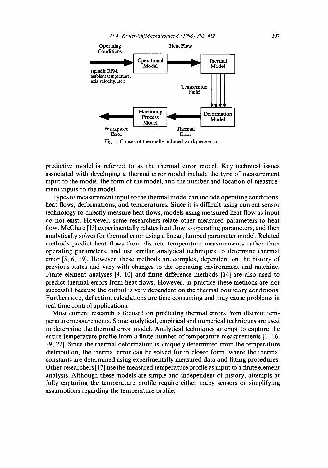
The causes of thermally induced workpiece errors are depicted in Fig. 1. The operating conditions are input to the operational model, producing heat flows. These heat flows are input to the heat model, producing varying temperature fields through the machine structure. The varying temperature fields are then input to the defor- mation model, producing thermally induced positioning errors of the tool with respect to the workpiece. This thermally induced error is referred to as thermal error. The thermal error is input to the machining process model that produces errors on the workpiece. The mathematical predictive model necessary to perform thermal error compensation predicts the thermal errors from measured inputs. The mathematical
D.A. Krulewich/Mechatronics 8 (1998) 395~412
Operating Heat Flow Conditions
I i Model (spindle RPM, I ambient temperature, axis velocity, etc.)
V
Temperatue Field
I Mach in ing ~.~ Process ..~
- " I Model Workpiece Thermal
Error Error Fig. 1. Causes of thermally induced workpiece error.
Thermal Model
L Ill Deformation
Model
397
predictive model is referred to as the thermal error model. Key technical issues associated with developing a thermal error model include the type of measurement input to the model, the form of the model, and the number and location of measure- ment inputs to the model.
Types of measurement input to the thermal model can include operating conditions, heat flows, deformations, and temperatures. Since it is difficult using current sensor technology to directly measure heat flows, models using measured heat flow as input do not exist. However, some researchers relate other measured parameters to heat flow. McClure [13] experimentally relates heat flow to operating parameters, and then analytically solves for thermal error using a linear, lumped parameter model. Related methods predict heat flows from discrete temperature measurements rather than operating parameters, and use similar analytical techniques to determine thermal error [5, 6, 19]. However, these methods are complex, dependent on the history of previous states and vary with changes to the operating environment and machine. Finite element analyses [9, 10] and finite difference methods [14] are also used to predict thermal errors from heat flows. However, in practice these methods are not successful because the output is very dependent on the thermal boundary conditions. Furthermore, deflection calculations are time consuming and may cause problems in real time control applications.
Most current research is focused on predicting thermal errors from discrete tem- perature measurements. Some analytical, empirical and numerical techniques are used to determine the thermal error model. Analytical techniques attempt to capture the entire temperature profile from a finite number of temperature measurements [1, 16, 19, 22]. Since the thermal deformation is uniquely determined from the temperature distribution, the thermal error can be solved for in closed form, where the thermal constants are determined using experimentally measured data and fitting procedures. Other researchers [17] use the measured temperature profile as input to a finite element analysis. Although these models are simple and independent of history, attempts at fully capturing the temperature profile require either many sensors or simplifying assumptions regarding the temperature profile.
398 D.A. Krulewich/Mechatronics 8 { 1998) 395~412
Purely empirical models also exist that relate discrete temperature measurements to thermal deformation. Empirical models can use an assumed linear form for the thermal error model and statistical techniques to fit the model. Most of these models are independent of the temperature history [3, 4, 11, 12, 18, 19, 22], but a few are history dependent [8, 19]. Some are dependent on operating conditions, so a different model is required for warm-up and cool-down situations. The simplest models contain only first order terms, while more complex models contain higher order powers of the measured temperatures and interaction terms between the measured temperatures. Statistical techniques (step-wise linear regression, the F-statistic, Mallows Cp statistic and the correlation coefficient) are used to determine the optimum terms in the model.
Neural networks are also a popular technique used to develop empirical models between discrete temperature measurements and thermal errors [2, 3, 15, 20 24]. These models tend to be complex and highly non-linear. The model predictions have the potential to very accurately track the training conditions, but may diverge significantly from the physical output during other conditions. Therefore large amounts of training data are required to adequately fit the model for all possible conditions.
All empirical thermal error models face similar weaknesses. First, the models lack relation to the actual physical situation. As noted by Fraser [5], since the empirically based functions bear no physical similarity to the actual function, lots of data are required to adequately fit these models, and the models do not extrapolate well outside the measured conditions.
Second, the accuracy of the thermal error model prediction is highly dependent on the placement and number of discrete temperature measurements. Many researchers are focusing on developing methodologies for optimum sensor placement, but there is no method that has shown universal success in an industrial environment. In some cases, the placement and number of sensors are determined using engineering judgment, often placing the sensors near the heat sources [2, 4, 11, 17, 20]. Because the thermal capacitance of the machine structure, the temperatures of the sources are related to the deformation in a history dependent non-linear manner. Often the assumed form of the model does not account for these history dependencies and non- linearities. Other researchers place a large number of sensors on the machine structure and use techniques to select the optimum subset of sensors. Some researchers use statistical techniques to select the optimum subset of sensors [3, 12, 23], and others select the most sensitive locations where the change in thermal deflection with respect to change in temperature is the greatest [24]. These selection processes usually require large amounts of data, temperature sensors, and time and are often not practical to the common machine user. Furthermore, it is not apparent that the optimum sensors for one particular machine are the same optimum sensors for another machine of the same model but in a different operating environment.
It is also possible to predict thermal errors from measured deformations throughout the machine structure. A linear model relating machine deformations to the tool point deflection is empirically developed in [7]. This method poses similar problems regarding where to place the deflection sensors and how many sensors are required.
D.A. Krulewich/Mechatronics 8 (1998) 395-412 399
Furthermore, the model is purely empirical and therefore requires a large amount of training data and does not extrapolate well beyond the measured ranges.
For these reasons, this work focuses on developing a model with a base function related to the physical situation. Furthermore, we have developed a method to deter- mine the number and location of temperature measurements for this model. In the remainder of this paper, the technical approach will be described followed by experimental verification where the thermal errors of a spindle are characterized. We also include a comparison between this method and a statistical approach, showing that this method is as good as if not better than this particular statistical approach. The advantage is not as much in overall accuracy but in an increase in robustness and a reduction in the required collection time and amount of data.
Technical approach
The heart of this approach is based on the assumption that the temperature dis- tribution in a particular region on a machine can be estimated by a polynomial. Polynomial temperature distributions have also been assumed in other research [1, 19]. However, previous work has required as many as 100 temperature sensors [1] to capture the entire temperature distribution. To remedy this problem, we rely on the fact that the thermal error is related to the integral of the temperature profile rather than the entire temperature profile itself. It is therefore not necessary to capture the entire temperature profile.
The form of the model is derived from the analytical integral solution, accomplished by numerically integrating the temperature profile. This approach is attractive in that a simple linear model is produced that is related to the analytical solution, thus producing a robust model that has good tracking capability. Furthermore, less data are required to fit this model and the model has better extrapolating abilities.
The location and number of required temperature measurements are directly tied to the type of numerical integration. There are many common forms of numerical integration such as the Forward and Backward Cauchy Euler methods. However, Gaussian integration produces the exact solution with the minimum number of points. Furthermore, the location of the numerical integration points are independent of the coefficients of the polynomial and dependent only on the order of the polynomial. If we assume that as operating conditions change, the coefficients of the temperature profile polynomial change but the order of the polynomial is always equal to or less than a finite value, then Gaussian integration will produce exact result regardless of operating conditions. Therefore, the same model will track under varying operating conditions, including warm-up and coot-down cycles as well as changing velocities and environmental conditions.
Simplified one-dimensional heat f low
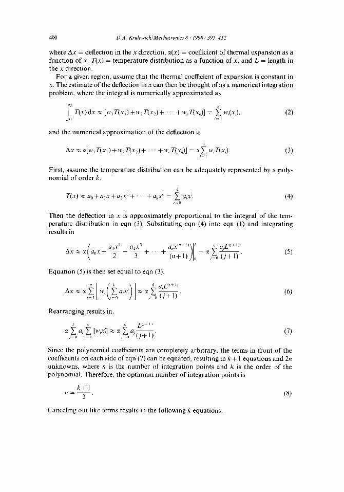
The one-dimensional deflection caused by a temperature distribution is
Ax = ~(x) T(x) dx ,.~ ~ T(x) dx o
(1)
400 D.A. Krulewich/ Mechalronics 8 (1998) 395-412
where Ax = deflection in the x direction, e(x) = coefficient of thermal expansion as a function of x, T(x) = temperature distribution as a function of x, and L = length in the x direction.
For a given region, assume that the thermal coefficient of expansion is constant in x. The estimate of the deflection in x can then be thought of as a numerical integration problem, where the integral is numerically approximated as
r ( x ) d x ~ [ w I T ( x , ) + w 2 T ( x 2 ) + ' " + w,,T(x,)] = wi(xi), (2) i=1
and the numerical approximation of the deflection is
A x ~ ~[w~ T ( x , ) + w 2 T ( x 2 ) + " " + w.,T(x.)] = a ~ w~T(x~). i=1
(3)
First, assume the temperature distribution can be adequately represented by a poly- nomial of order k,
k
T(x) ,~ ao-t-alx +a2x2 + . . . +al,,x k = 2 ajx'. (4) j= 0
Then the deflection in x is approximately proportional to the integral of the tem- perature distribution in eqn (3). Substituting eqn (4) into eqn (1) and integrating results in
al X2 a2 X3 anXl,~+l)~L = k aL(J+l) ~J~
A x ~ a 0 x + ~ + . 3 + " " + (n+l)//10 / ~ 0 ( j + l ) " (5)
Equation (5) is then set equal to eqn (3),
i=1 j i=0 ( J+ 1) (6)
Rearranging results in,
c¢ ~ aj Z [w~x~] ~ ~ ~ a, . (7) ~=o i=l /=o ( j + l )
Since the polynomial coefficients are completely arbitrary, the terms in front of the coefficients on each side ofeqn (7) can be equated, resulting in k + 1 equations and 2n unknowns, where n is the number of integration points and k is the order of the polynomial. Therefore, the optimum number of integration points is
k + l H - - (8)
Canceling out like terms results in the following k equations.
D.A. Krulewich/Mechatronics 8 (1998) 395-412 401
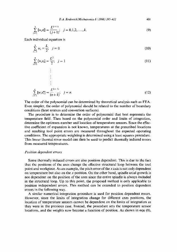
LO. + ~) i=l[WiXiJ]m(~)'~ j = 0,1,2 . . . . . k. (9)
Each individual equation is
,=1 w, = ~-; j = O ( io)
~] L2 i=1 [WiXi] = T ; j = 1 (11)
L(n+ l)
,=, [w,x~] = (n + 1~; j = n. (12)
The order of the polynomial can be determined by theoretical analysis such as FEA. Even simpler, the order of polynomial should be related to the number of boundary conditions (heat sources and convection surfaces).
The procedure is to determine the order of polynomial that best represents the temperature field. Then based on the polynomial order and limits of integration, determine the optimum number and location of temperature sensors. Since the effec- tive coefficient of expansion is not known, temperatures at the prescribed locations and resulting tool point errors are measured throughout the expected operating conditions. The appropriate weighting is determined using a least squares procedure. This linear thermal error model can then be used to predict thermally induced errors from measured temperatures.
Position dependent errors
Some thermally induced errors are also position dependent. This is due to the fact that the positions of the axes change the effective structural loop between the tool point and workpiece. As an example, the pitch error of the x axis is not only dependent on temperature but also on the x position. On the other hand, spindle axial growth is not dependent on the position of the axes since the entire spindle is always included in the structural loop. Up to this point, the proposed method is only applicable to position independent errors. This method can be extended to position dependent errors in the following way.
A similar numerical integration procedure is used for position dependent errors. However, since the limits of integration change for different axes positions, the location of temperature sensors cannot be dependent on the limits of integration as they were in the previous case. Instead, the procedure sets the temperature sensor locations, and the weights now become a function of position. As shown in eqn (8),
402 D.A. Kruh, wich/Mechatronics 8 (1998) 395--412
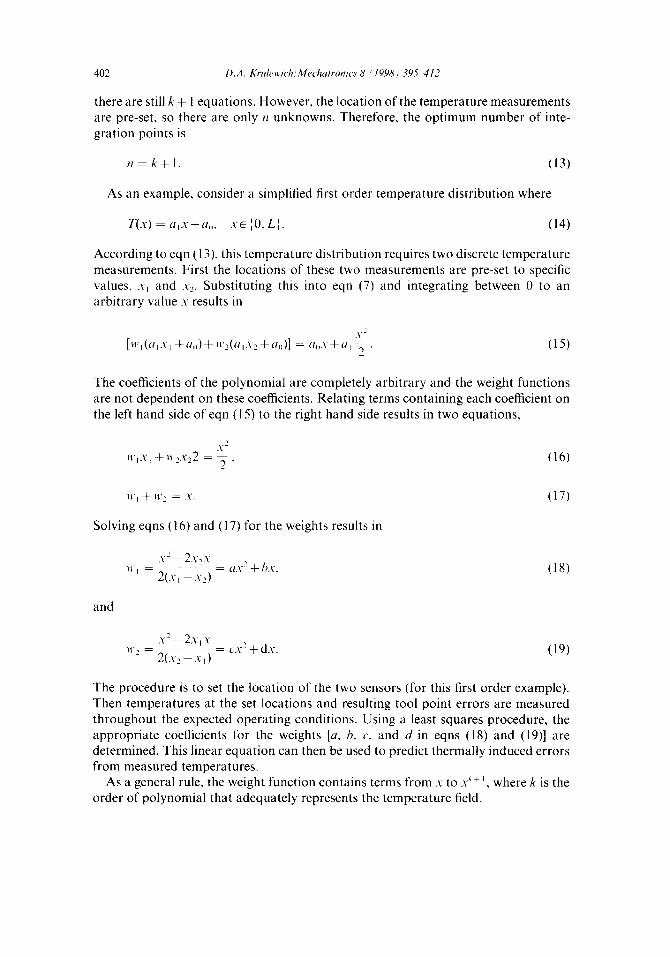
there are still k + 1 equations. However, the location o f the temperature measurements are pre-set, so there are only n unknowns. Therefore, the op t imum number o f inte- gration points is
n = k-t- 1. (13)
As an example, consider a simplified first order temperature distribution where
T ( . v ) = a , x + a , , xe{0 , L}. (14)
According to eqn (13), this temperature distribution requires two discrete temperature measurements. First the locations o f these two measurements are pre-set to specific values, .v~ and .\-~. Substituting this into eqn (7) and integrating between 0 to an arbitrary value x results in
.¥2
[ w l ( a lV l + a ° ) q - w 2 ( a i x 2 + a ° ) ] = g l ° x + ° l 9 " (15)
The coefficients o f the polynomial are completely arbitrary and the weight functions are not dependent on these coefficients. Relating terms containing each coefficient on the left hand side o f eqn (15) to the right hand side results in two equations,
X 2
wl-vt +w>v_,2 = 2 , (16)
wl +we = x. (17)
Solving eqns (16) and (17) for the weights results in
.v -~ - 2x,.v w, = 2(i;.-, Z.,-:) = a-'~ + h.,-. (18)
and
. C - 2 x , . v w2 . . . . . cx-" + d_v. (19)
2(X_~--Xl)
The procedure is to set the location of the two sensors (for this first order example). Then temperatures at the set locations and resulting tool point errors are measured th roughout the expected operat ing conditions. Using a least squares procedure, the appropria te coefficients for the weights [a, b, c, and d in eqns (18) and (19)] are determined. This linear equat ion can then be used to predict thermally induced errors f rom measured temperatures.
As a general rule, the weight function contains terms from .v to .v k+], where k is the order of polynomial that adequately represents the temperature field.

D.A. Krulewich/ Mechatronics 8 (1998) 395--412 403
Results
Two test set-ups have been designed. The purpose of the first set-up is to study this approach using a simple, one dimensional heat flow problem with a known, controlled heat source. The purpose of the second set-up is to apply this theory to an actual spindle.
Test set-up 1--aluminum tube
The first test stand consisted of a hollow, 305 mm aluminum tube mounted verti- cally, as shown in Fig. 2. One end was attached to a granite block while the other end was free. A capacitance gage was used to measure growth at the free end. A total of nine thermistors were mounted along the length of the tube, and the temperature of the granite block along with ambient temperature were also monitored.
A thin wire wrapped around the tube with current running through it was used as a single point heat source. Since there were two boundary conditions at the ends and one heat source, we initially assumed that the temperature profile could be represented by a third order polynomial. By eqn (8), two points are required for numerical integration. Nine temperature sensors were placed along the length of the aluminum tube, two of which were placed at the Gaussian integration points. The extra sensors were used to (1) verify that the temperature profile could be adequately represented by a third order polynomial, and (2) compare a statistical approach to the proposed approach. Axial growth was measured for the heat source located 222 mm from the granite block. Temperature and growth measurements were taken while maximum current was applied for 20 min. Then the heat source was removed and data were taken for 20 min more while the aluminum tube cooled.
Five additional sets of data were acquired for model verification, using equal or less current through the heated wire. For comparison, a statistical approach was used to select the optimum two temperature sensors. The statistical approach selected the two temperature sensors that minimized the sum squared error of the training set. The statistical approach selected the same optimum sensor locations as the Gaussian
capacitance gage
A hermistor
aluminum tube
Fig. 2. Test set-up 1.
404 D.A. Krulewich/ Mechatronics 8 (1998) 395-412
integration approach. Between 94.4 98.8 percent of the measured axial growth was predicted by the model for each of the five data sets.
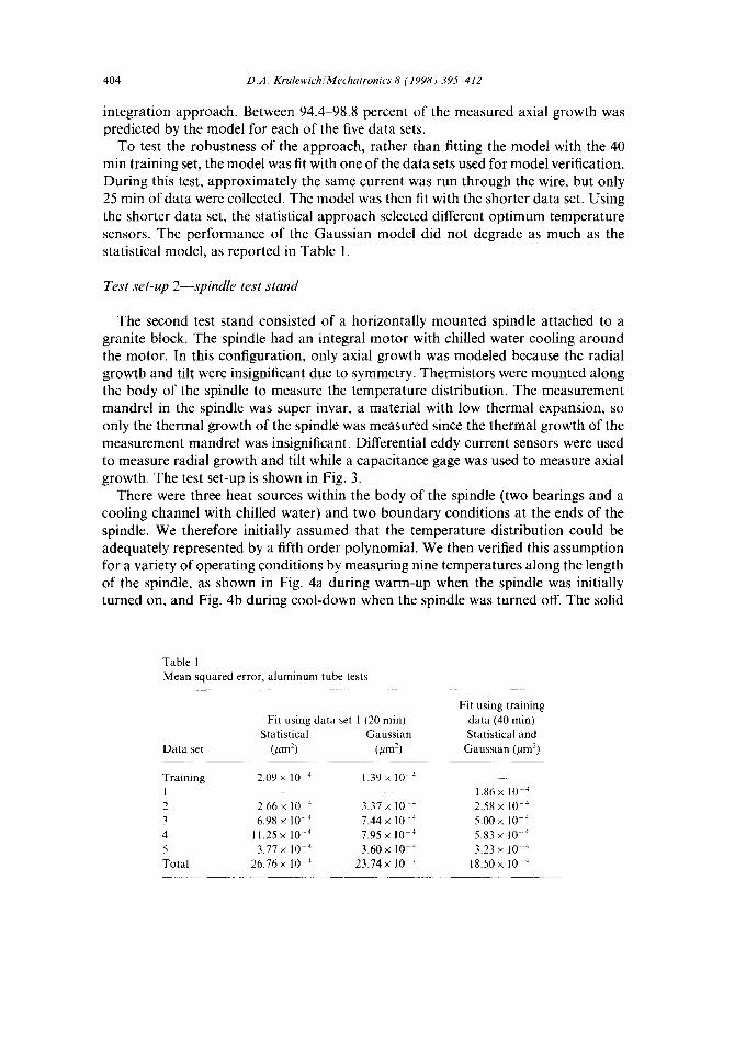
To test the robustness of the approach, rather than fitting the model with the 40 min training set, the model was fit with one of the data sets used for model verification. During this test, approximately the same current was run through the wire, but only 25 min of data were collected. The model was then fit with the shorter data set. Using the shorter data set, the statistical approach selected different optimum temperature sensors. The performance of the Gaussian model did not degrade as much as the statistical model, as reported in Table 1.
Test set-up 2--spindle test stand
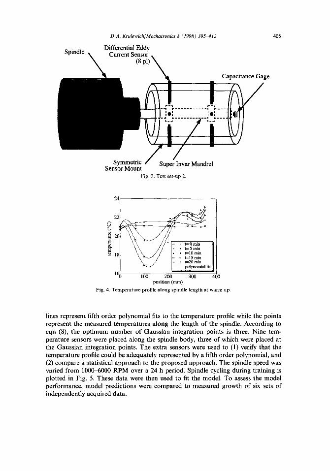
The second test stand consisted of a horizontally mounted spindle attached to a granite block. The spindle had an integral motor with chilled water cooling around the motor. In this configuration, only axial growth was modeled because the radial growth and tilt were insignificant due to symmetry. Thermistors were mounted along the body of the spindle to measure the temperature distribution. The measurement mandrel in the spindle was super invar, a material with low thermal expansion, so only the thermal growth of the spindle was measured since the thermal growth of the measurement mandrel was insignificant. Differential eddy current sensors were used to measure radial growth and tilt while a capacitance gage was used to measure axial growth. The test set-up is shown in Fig. 3.
There were three heat sources within the body of the spindle (two bearings and a cooling channel with chilled water) and two boundary conditions at the ends of the spindle. We therefore initially assumed that the temperature distribution could be adequately represented by a fifth order polynomial. We then verified this assumption for a variety of operating conditions by measuring nine temperatures along the length of the spindle, as shown in Fig. 4a during warm-up when the spindle was initially turned on, and Fig. 4b during cool-down when the spindle was turned off. The solid
Table 1
M e a n squared error , a l u m i n u m tube tests
Fit using t ra ining
Fit using da t a set 1 (20 rain) da t a (40 min)
Statistical Gauss ian Statistical and D a t a set ( / / m 2 ) ( l l m 2 ) Gauss ian (pm 2)
Tra in ing 2.09 x 10 4 1.39 x 10 4
1 1 . 8 6 z 10 4
2 2 . 6 6 × 1 0 4 3 . 3 7 × 1 0 4 2 , 5 8 x 1 0 4
3 6 . 9 8 x 1 0 4 7 . 4 4 x 1 0 4 5 . 0 0 x 1 0 4
4 11.25 x 10 4 7.95 × 10 -4 5.83 x 10 4
5 3.77 x 10 4 3.60 x 10 4 3.23 x 10 4
T o t a l 2 6 . 7 6 x 10 4 2 3 . 7 4 x 10 4 1 8 . 5 0 x 10 4
qnlnAl,~
D.A. Krulewich / Mechatronics 8 (1998) 395-412
Differential Eddy
405
ge
S e n s o r M o u n t ~ ' u v " . . . . . . " ' ' " . . . .
Fig. 3. Test set-up 2.
24
22
oC 20
~ \ / / I~ ~ t=Smin o 18 \ \ / ! I ' 0 t=lOmin
\ ~ / I D o t=15min / [~ * t=20min
I - - polynomial fit
164 100 200 300 400 position (mm)
Fig. 4. Tempera ture profile along spindle length at wa rm up.
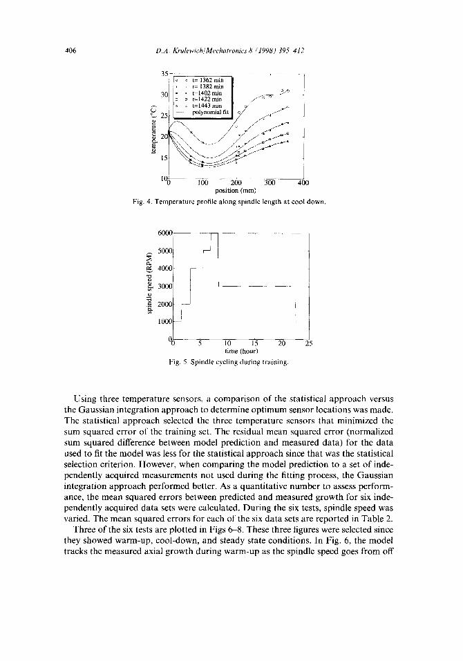
lines represent fifth order polynomial fits to the temperature profile while the points represent the measured temperatures along the length of the spindle. According to eqn (8), the optimum number of Gaussian integration points is three. Nine tem- perature sensors were placed along the spindle body, three of which were placed at the Gaussian integration points. The extra sensors were used to (1) verify that the temperature profile could be adequately represented by a fifth order polynomial, and (2) compare a statistical approach to the proposed approach. The spindle speed was varied from 1000-6000 RPM over a 24 h period. Spindle cycling during training is plotted in Fig. 5. These data were then used to fit the model. To assess the model performance, model predictions were compared to measured growth of six sets of independently acquired data.
406 D.A. Krulewich/Mechatronics 8 (1998) 395~412
351 ~ = 1~62 min~-- I . . . . . /1+ + t=1382min | o
30[ l" , t=1402min I " [[= D t=142Zmin [ / ~ - o o
[~ ~ t=1443min | 9 / ../, °~ 25 I - - polynomialfit 1 / / / . ~
1( 1 O0 200 300 400 position (mm)
Fig. 4. Temperature profile along spindle length at cool down.
6 0 0 0 - - + ~ . . . . . . . . . ~ - - - -
5ooo j i 4ooo ' I
F -¸ -+ 1 = 2000 r- J
looo I o
00 5 10 1 '5 2'0 time (hour)
Fig. 5. Spindle cycling during training.
I
r
. . . . .
25
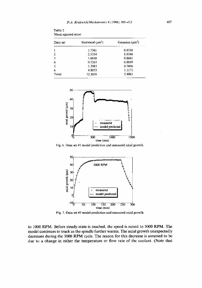
Using three temperature sensors, a comparison of the statistical approach versus the Gaussian integration approach to determine optimum sensor locations was made. The statistical approach selected the three temperature sensors that minimized the sum squared error of the training set. The residual mean squared error (normalized sum squared difference between model prediction and measured data) for the data used to fit the model was less for the statistical approach since that was the statistical selection criterion. However, when comparing the model prediction to a set of inde- pendently acquired measurements not used during the fitting process, the Gaussian integration approach performed better. As a quantitative number to assess perform- ance, the mean squared errors between predicted and measured growth for six inde- pendently acquired data sets were calculated. During the six tests, spindle speed was varied. The mean squared errors for each of the six data sets are reported in Table 2.
Three of the six tests are plotted in Figs 6-8. These three figures were selected since they showed warm-up, cool-down, and steady state conditions. In Fig. 6, the model tracks the measured axial growth during warm-up as the spindle speed goes from off
D.A. Krulewich/ Mechatronics 8 (1998) 395-412
Table 2 Mean squared error
Data set Statistical (#m 2) Gaussian (#m 2)
1 1.7361 0.8338 2 2.5334 1.0346 3 1.0038 0.8641 4 0.7263 0.8859 5 1.3985 0.7606 6 4.8055 1.1171 Total 12.3036 5.4961
407
50
40
:3. 30
~ 20
10
500 10~)0 1500 time (min)
Fig. 6. Data set #1 model prediction and measured axial growth.
50
40
30
20 .o
(
-1(
o__ me~ur~ ] model predicted
50 100 150 200 250 300 time (rain)
Fig. 7. Data set #3 model prediction and measured axial growth.
to 1000 RPM. Before steady-state is reached, the speed is raised to 5000 RPM. The model continues to track as the spindle further warms. The axial growth unexpectedly decreases during the 5000 RPM cycle. The reason for this decrease is assumed to be due to a change in either the temperature or flow rate of the coolant. (Note that
408 D . A . K r u l e w i c h / M e c h a t r o n i c s 8 ( 1 9 9 8 ) 3 9 5 - 4 1 2
5 0 - - T ..... ,~ ,
2500 RPM 4 ~ ~ 5 ~ RPM
'~ ° measured I 10 - - model predicted ~
c
(~ IO0 200 300 400 500 time (min)
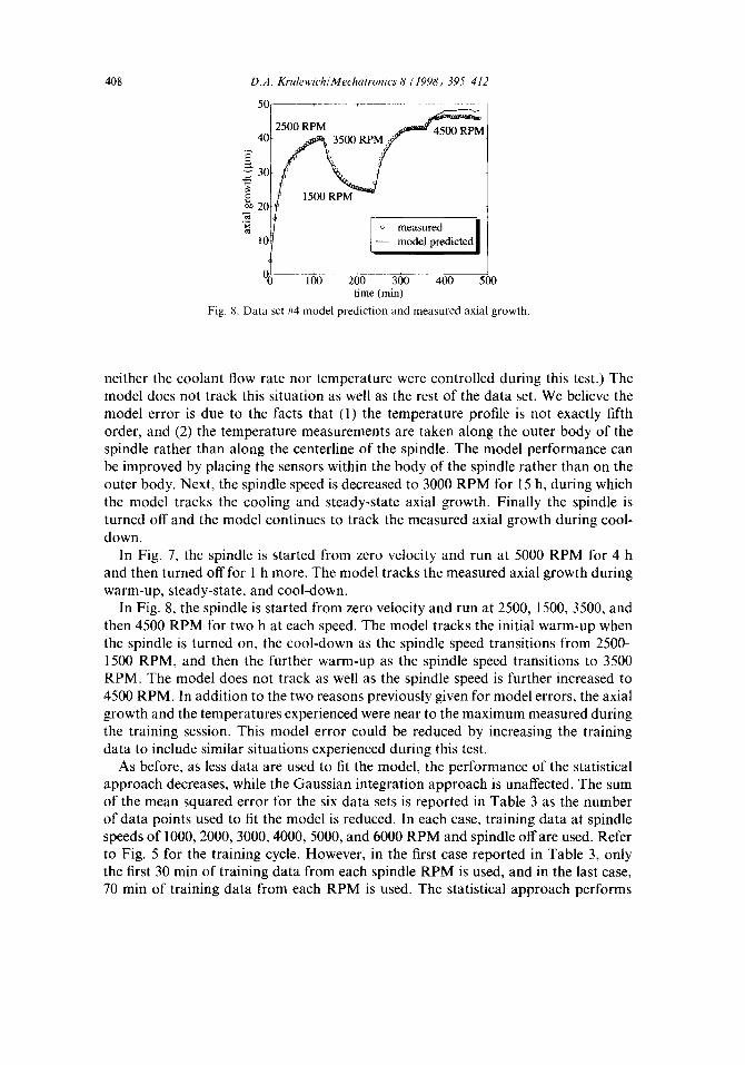
Fig. 8. Data set #4 model prediction and measured axial growth.
neither the coolant flow rate nor temperature were controlled during this test.) The model does not track this situation as well as the rest of the data set. We believe the model error is due to the facts that (1) the temperature profile is not exactly fifth order, and (2) the temperature measurements are taken along the outer body of the spindle rather than along the centerline of the spindle. The model performance can be improved by placing the sensors within the body of the spindle rather than on the outer body. Next, the spindle speed is decreased to 3000 RPM for 15 h, during which the model tracks the cooling and steady-state axial growth. Finally the spindle is turned off and the model continues to track the measured axial growth during cool- down.
In Fig. 7, the spindle is started from zero velocity and run at 5000 RPM for 4 h and then turned off for 1 h more. The model tracks the measured axial growth during warm-up, steady-state, and cool-down.
In Fig. 8, the spindle is started from zero velocity and run at 2500, 1500, 3500, and then 4500 RPM for two h at each speed. The model tracks the initial warm-up when the spindle is turned on, the cool-down as the spindle speed transitions from 2500- 1500 RPM, and then the further warm-up as the spindle speed transitions to 3500 RPM. The model does not track as well as the spindle speed is further increased to 4500 RPM. In addition to the two reasons previously given for model errors, the axial growth and the temperatures experienced were near to the maximum measured during the training session. This model error could be reduced by increasing the training data to include similar situations experienced during this test.
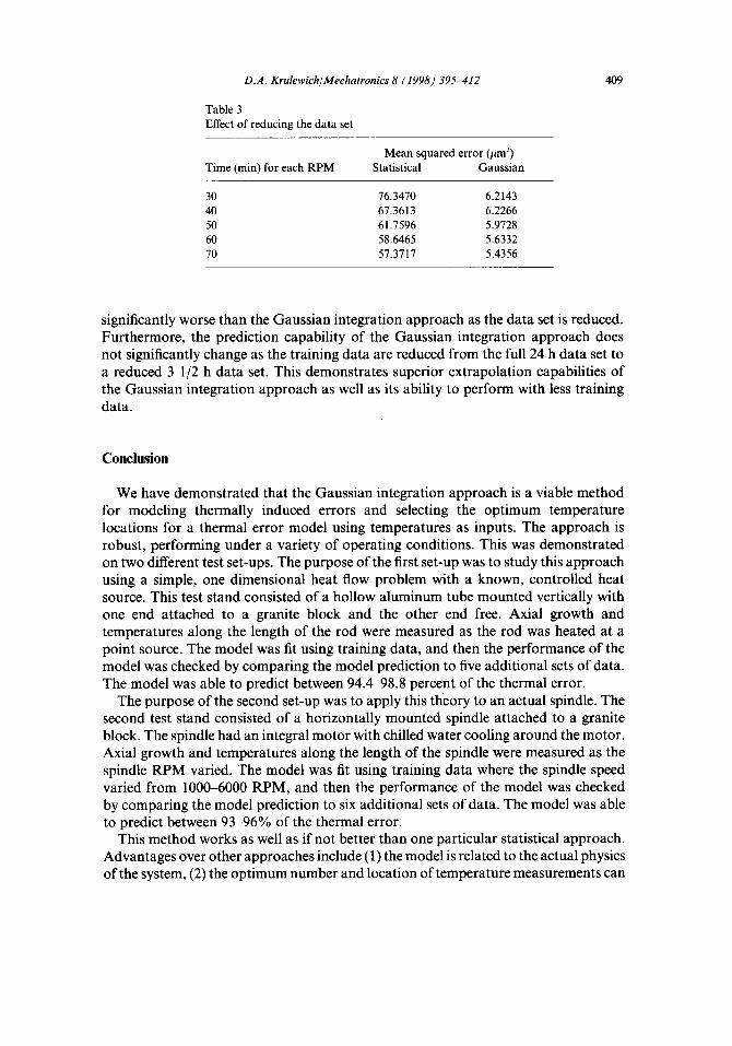
As before, as less data are used to fit the model, the performance of the statistical approach decreases, while the Gaussian integration approach is unaffected. The sum of the mean squared error for the six data sets is reported in Table 3 as the number of data points used to fit the model is reduced. In each case, training data at spindle speeds of 1000, 2000, 3000, 4000, 5000, and 6000 RPM and spindle off are used. Refer to Fig. 5 for the training cycle. However, in the first case reported in Table 3, only the first 30 min of training data from each spindle RPM is used, and in the last case, 70 min of training data from each RPM is used. The statistical approach performs
D.A. Krulewich/ Mechatronics 8 (1998) 395-412
Table 3 Effect of reducing the data set
Mean squared error (ktm 2) Time (min) for each R P M Statistical Gauss ian
30 76.3470 6.2143 40 67.3613 6.2266 50 61.7596 5.9728 60 58.6465 5.6332 70 57.3717 5.4356
409
significantly worse than the Gaussian integration approach as the data set is reduced. Furthermore, the prediction capability of the Gaussian integration approach does not significantly change as the training data are reduced from the full 24 h data set to a reduced 3 1/2 h data set. This demonstrates superior extrapolation capabilities of the Gaussian integration approach as well as its ability to perform with less training data.
Conclusion
We have demonstrated that the Gaussian integration approach is a viable method for modeling thermally induced errors and selecting the optimum temperature locations for a thermal error model using temperatures as inputs. The approach is robust, performing under a variety of operating conditions. This was demonstrated on two different test set-ups. The purpose of the first set-up was to study this approach using a simple, one dimensional heat flow problem with a known, controlled heat source. This test stand consisted of a hollow aluminum tube mounted vertically with one end attached to a granite block and the other end free. Axial growth and temperatures along the length of the rod were measured as the rod was heated at a point source. The model was fit using training data, and then the performance of the model was checked by comparing the model prediction to five additional sets of data. The model was able to predict between 94.4-98.8 percent of the thermal error.
The purpose of the second set-up was to apply this theory to an actual spindle. The second test stand consisted of a horizontally mounted spindle attached to a granite block. The spindle had an integral motor with chilled water cooling around the motor. Axial growth and temperatures along the length of the spindle were measured as the spindle RPM varied. The model was fit using training data where the spindle speed varied from 1000qS000 RPM, and then the performance of the model was checked by comparing the model prediction to six additional sets of data. The model was able to predict between 93-96% of the thermal error.
This method works as well as if not better than one particular statistical approach. Advantages over other approaches include (1) the model is related to the actual physics of the system, (2) the optimum number and location of temperature measurements can
410 D.A. Krulewich/Mechatronics 8 (1998) 395~12
be determined without acquiring any data, and (3) less data are required to train the model.
The thermal model is related to the actual physics of the system since its form was derived from Gaussian numerical integration assuming a polynomial temperature profile. Since the model is related to the actual system, less training data are required and the model has better extrapolation capabilities than a purely empirical model. Furthermore, the thermal model presented in this paper is a simple linear function of temperature measurements. This linear model is advantageous over more complex, non-linear models since (l) simple models are easier to implement and (2) linear models have better extrapolation capabilities than models with higher order terms and non-linearieties.
The opt imum number and location of temperature measurements is intrinsically related to the form of the model for the thermal model developed in this paper. The opt imum temperature measurements are selected as the Gaussian integration points along an assumed polynomial temperature profile. The location is dependent only on the order of the temperature profile polynomial and not on the coefficients of the polynomial. The key assumption is that as the operating conditions change, the coefficients of the polynomial change but the order of the polynomial is always equal to or less than a finite number. Given this assumption, this model should track under all operating conditions. This model robustness was verified on the two test set-ups, where the model was able to track actual thermal growth under varying operating conditions.
It should be further noted that some alternative approaches require the machine to be fixtured with many extra temperature sensors during the fitting procedure. Then after data are taken, techniques are used to determine the opt imum subset of tem- perature sensor locations and possibly the opt imum terms in the model. The assump- tion is then made that the optimum sensor locations for the one machine used during initial testing are the same opt imum sensor locations for all machines with the same configuration. For this assumption to be valid, large amounts of data must be taken that covers the full range of operating conditions. Furthermore, it may not be possible to perform the initial testing with so many sensors in an industrial environment.
We verified that less data are required to train the model by reducing the number of points from the training sets for both test set-ups. In both cases, the performance of the Gaussian integration approach remained approximately the same while the performance of the statistical approach drastically decreased as the size of the training data was reduced.
It should be noted that thermal error compensation does not replace the need for a thermally controlled environment or a well designed machine. On the contrary, the validity of certain assumptions are highly dependent on well maintained environments and good designs.
Future work
To implement this approach on a machine, we must first determine a method to divide the machine into subsystems. The thermal growth of each subsystem will then
D.A. Krulewich/Mechatronics 8 (1998) 395 412 411
be de te rmined by this p r o p o s e d approach . The subsys tems will be re la ted to the c o m p o n e n t s tha t create the k inemat ic loop f rom the tool to the workpiece . Con t inu i ty between subsys tem t empera tu re profiles mus t be addressed as well as t r ans la t ion and ro ta t ion between ind iv idua l subsystems. Next we mus t develop a m e t h o d to de te rmine the highest o rde r po lynomia l tha t can adequa te ly represent the t empera tu re profile under vary ing ope ra t ing condi t ions . This m e t h o d ideal ly will not require add i t iona l t empera tu re measurements . Instead, the po lynomia l o rde r will be di rect ly re la ted to the loca t ion and n u m b e r o f b o u n d a r y cond i t ions on the ind iv idua l unit. The n u m b e r and loca t ion o f t empera tu re measurement s will then be de te rmined by the o rde r of the po lynomia l s . F ina l ly , each c o m p o n e n t thermal e r ror will be summed th rough the k inemat ic loop to p roduce a tool po in t with respect to workpiece error . M o d e l coefficients will be de te rmined by measur ing the discrete t empera tu res and the tool po in t e r ror as the machine is cycled th rough typical mach in ing condi t ions .
To remove the er rors in real t ime, the cont ro l le r mus t have the capabi l i ty o f acqui r ing the t empera tu re measurements , ca lcula t ing the c ompe nsa t i on values and then cor rec t ing the mot ion . A l t h o u g h open archi tec ture cont ro l le rs are beginning to appea r on the marke t , mos t cont ro l le rs are "c losed" , so the con t ro l a lgor i thm canno t be al tered. F u r t h e r m o r e , m a n y machines do no t have an angu la r axis tha t can remove the tilt tha t can cause er rors dur ing dr i l l ing or bor ing opera t ions . Therefore , we are cons ider ing an a l ternat ive a p p r o a c h where the spindle coo lan t t empera tu re and flow rate are external ly con t ro l l ed to minimize the rad ia l and axial m o t i o n o f the spindle. The tilt m o t i o n o f the spindle can also be con t ro l l ed by designing a p p r o p r i a t e cool ing channels on a new spindle.
We are also interested in co l l abo ra t i on to c ompa re this m e t h o d to a neural ne twork a p p r o a c h a long with o ther s tat is t ical approaches .
References
[1] Balsamo A, Marques D, Satori S. A method for thermal-deformation corrections of CMMs. Annals of the CIRP 1990;39(1):557~60.
[2] Chen JS, Chiou G, Quick testing and modeling of thermally-induced errors of CNC machine tools. International Journal of Machine Tools & Manufacture 1995;35(7): 1063-74.
[3] Chen J, Yuan J, Ni J, Wu SM. Thermal error modeling for volumetric error compensation. Winter Annual Meeting of the American Society of Mechanical Engineers, Sensors and Signal Processing for Manufacturing American Society of Mechanical Engineers, Production Engineering Division 1992;55:113 25.
[4] Fan K, Lin F, Lu S. Measurement and compensation of thermal error on a machining center. Proceedings of the 9th International MATADOR Conference 1992;261 8.
[5] Fraser S, Attia M, Osman M. Modeling, identification and control of thermal deformation of machine tool structures: Part l~oncep t of generalized modeling. Proceedings of the 1994 International Mechanical Engineering Congress and Exposition Conference, Manufacturing Science and Engin- eering American Society of Mechanical Engineers, Production Engineering Division 1994;68(2):931 44.
[6] Fraser S, Osman M, Attia M. Modeling, identification and control of thermal deformation of machine tool structures: Part II--generalized transfer functions. Proceedings of the 1994 International Mech- anical Engineering Congress and Exposition 1994;68(2):945-53.
[7] Hatamura Y, Nagao T, Mitsuishi M, Kato K, Taguchi S, Okumura T, Nakagawa G, Sugishita

412 I).A. Krulewich Mechatronics ~; 11998) 395-412
H. Development of an intelligent machining centcr incorporating active compensation for thermal distortion, Annals of the CI RP 1993:4( 1 ):549 52.
[8] Janeczko J, Machine tool thermal distortion compensation. 4th Biennial International Manul;acturing Technology Conference 1988:7D:7-167 7-181.
[9] Jedrzejewski J, Kaczmarek J, Kowal Z, Winiarski Z, Numerical optimization of thermal behaviour of machine tools. Annals of the CIRP 1990:39( 1 ):379 82.
[10] Jedrzejewski J, Modrzycki W. A new approach to modeling thermal behaviour of a machine tool under service conditions. Annals of the CIRP 1992:41( 1 ):455 8.
[1 I] Kurtoglu A. The accuracy improvement of machine tools. Annals of the CIRP 1990;39( 1):417 9. [12] Lo Hhih-Hao, Yuan Jingxia, Ni J. Optimal modeling of thermal error components for machine tool
error compensation. S.M. Wu Symposium 1994;1:000 000. [13] McClure R, Weck M, Petuelli G. Thermally induced errors. Technology of Machine Tools 1980;5:9.6-
1-9.6-23. [14] M~riwaki T. Therma~ def~rmati~n and its ~n-fine c~mpensati~n ~f hydr~statica~y supp~rted precisi~n
spindle. Annals of the CIRP 1988:37( I ):393 6. [I 5] Moriwaki T, Zhao C. Neural network approach to identify thermal deformation of machining center.
Proceedings of the 8th International IFIP TC5-WG5.3 Conference, Human Aspects in Computer Integrated Manufacturing 1992:685 97.
[16] Sartori S. A method tbr the identification and correction of thermal deformations in a three coordinate measuring machine. VDI Berichte 1989:761 : t 85 92.
[17] Schalz K. Improved thermal error compensation (TE(') o fCMM's . VDI Berichte 1989;761:177 84. [18] Schmidt J, Minges R. Thermal displacements at machine tools part 2: measurements and possible
compensation on a 3-axial NC milling machine. Werkstattstechnik Zeitschrift Fur lndustrielle Fer- tigung 1990;80(10):577 80.
[19] Soons J, Spaan H, Schellekens P. Thermal error models l'or software compensation of machine tools. ASPE Proceedings, Annual Meeting 1994:10:69 75.
[20] Veldhuis S, Elbestawi M. Modeling and compensation l;,~r five-axis machine tool errors. Proceedings of the 1994 International Mechanical Engineering Congress and Exposition Conference, Manufacturing Science and Engineering American Society of Mechanical Engineers, Production Engineering Division (Publication) PED 1994:68(2):827 39.
[2 I] Veldhuis S, Elbestawi M. A strategy for the compensation of errors in five-axis machining. Annals of the CIRP 1995;44(I):373 7.
[22] Venugopal R, Barash M. Thermal elt"ecls un the accuracy of numerically controlled machine tools. Annals of the CIRP 1986:35( 1 ):255 8.
[23] Yang S, Yuan J, Ni ,I. The improvement of thermal crror modeling and compensation on machine tools by CMAC neural network. International Journal of Machine Tools and Manufacture 1996:36(4):527 37.
[24] Zhang D, Liu X, Sfii H, Chen R. Identification of position of key thermal susceptible points for thermal error compensation of machine tool by neural network. Proceedings of SPIE The Inter- national Society for Optical Engineering Int. Conference on Intelligent Manufacturing 1995:2620:468 72.