teaching portfolio - bacalfa.combacalfa.com/calfaba-teachingportfolio.pdfteachingportfolio...

Teaching Portfolio Bruno Abreu Calfa

Teaching PortfolioBruno Abreu Calfa

January 29, 2015

ContentsTeaching Responsibilities 1

Teaching Philosophy 2

Sample Teaching Materials 4

Honors and Awards 4

Appendix A Course Syllabus: Numerical Methods in Engineering 5

Appendix B MATLAB Tutorial: Fall 2011 9

Appendix C Guest Lectures on Climate Change: Fall 2013 18

Appendix D Teaching Assistant Award Text: Academic Year 2011-2012 36

Teaching ResponsibilitiesAs a Ph. D. student in the Department of Chemical Engineering at Carnegie Mellon Univer-sity (CMU), I served as a teaching assistant (TA) in almost every semester of the program.I officially and unofficially assisted students from freshman to senior years. This was largelybecause I was the department’s “Math Software TA” for three times. This TA position en-abled me to provide help to undergraduate (and sometimes Master’s) students with regardsto software packages, such as MATLAB, Microsoft Excel, AspenPlus and others. This ex-perience was pedagogically very enriching to me as it allowed me to interact with studentsfrom different years and, thus, understand better the most common hurdles they faced acrossmultiple chemical engineering courses.

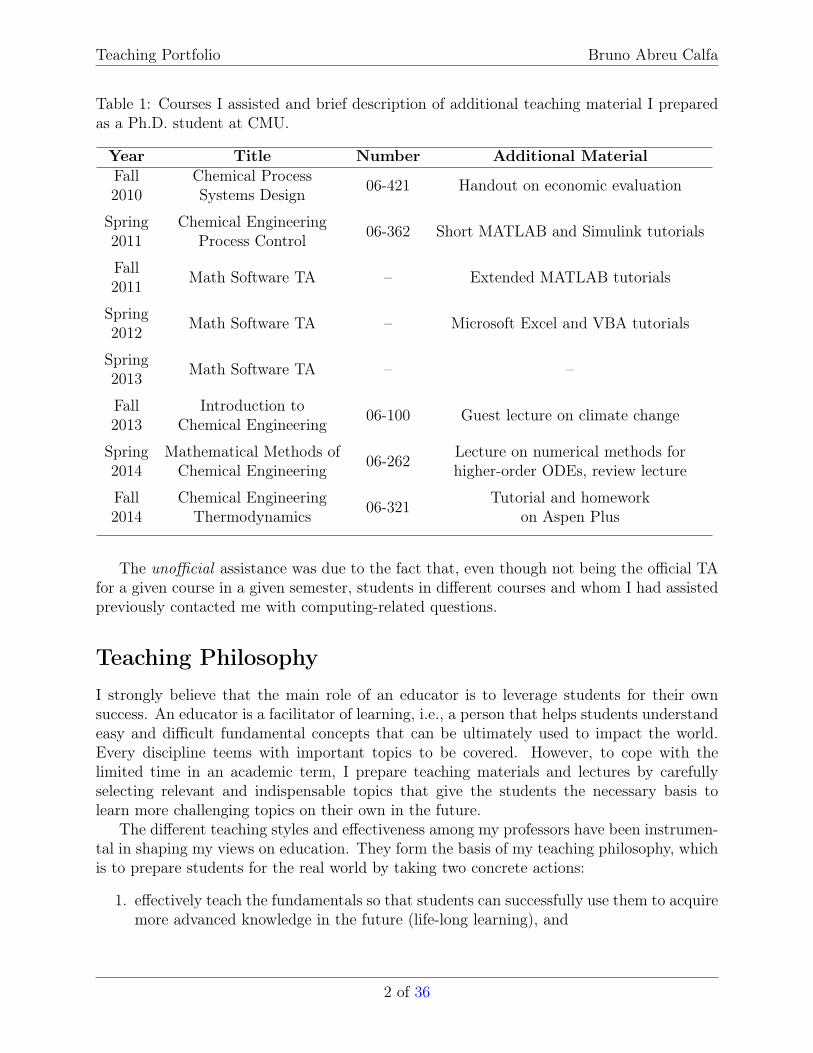
Table 1 summarizes the courses I served as a TA during my Ph.D. program. The column“Additional Material” lists the materials and activities I prepared and executed beyond thebasic TA requirements, such as grading homework and holding office hours. All materi-als can be retrieved from my personal website: http://bacalfa.com/TA/ExtraMaterial/TAExtraMaterial.html. The appendices contain the learning materials I prepared for someof the courses listed below.

1 of 36

http://bacalfa.com/TA/ExtraMaterial/TAExtraMaterial.html

http://bacalfa.com/TA/ExtraMaterial/TAExtraMaterial.html


Table 1: Courses I assisted and brief description of additional teaching material I preparedas a Ph.D. student at CMU.

Year Title Number Additional MaterialFall Chemical Process 06-421 Handout on economic evaluation2010 Systems Design

Spring Chemical Engineering 06-362 Short MATLAB and Simulink tutorials2011 Process Control

Fall Math Software TA – Extended MATLAB tutorials2011

Spring Math Software TA – Microsoft Excel and VBA tutorials2012

Spring Math Software TA – –2013

Fall Introduction to 06-100 Guest lecture on climate change2013 Chemical Engineering

Spring Mathematical Methods of 06-262 Lecture on numerical methods for2014 Chemical Engineering higher-order ODEs, review lecture

Fall Chemical Engineering 06-321 Tutorial and homework2014 Thermodynamics on Aspen Plus

The unofficial assistance was due to the fact that, even though not being the official TAfor a given course in a given semester, students in different courses and whom I had assistedpreviously contacted me with computing-related questions.

Teaching PhilosophyI strongly believe that the main role of an educator is to leverage students for their ownsuccess. An educator is a facilitator of learning, i.e., a person that helps students understandeasy and difficult fundamental concepts that can be ultimately used to impact the world.Every discipline teems with important topics to be covered. However, to cope with thelimited time in an academic term, I prepare teaching materials and lectures by carefullyselecting relevant and indispensable topics that give the students the necessary basis tolearn more challenging topics on their own in the future.

The different teaching styles and effectiveness among my professors have been instrumen-tal in shaping my views on education. They form the basis of my teaching philosophy, whichis to prepare students for the real world by taking two concrete actions:

1. effectively teach the fundamentals so that students can successfully use them to acquiremore advanced knowledge in the future (life-long learning), and

2 of 36


2. assess the students’ progress by assigning homework and projects that require bothindividual and group work plus in-class presentations (communication skills).

When I teach, I experience personal joy and satisfaction from helping someone understandsomething I also understand. In addition to that main driver, I have realized that teaching isalso a learning experience for me since each student has an individual approach to processingthe material, which requires flexibility from the instructor’s part.

From a practical viewpoint, I believe that educators equip students with fundamental, yetincomplete knowledge about the world, and that constitutes their toolbox. From personalexperience, students in general may not have the necessary maturity to comprehend thisfact until after they graduate. Once they graduate, they will be able to use the tools andskills from their toolbox to help them tackle real-world problems. A key aspect to thistoolbox is that students will know where to look for information when confronted withproblems, and motivate them to keep always learning. For instance, when teaching conceptsin Thermodynamics, such as fugacity and activity coefficients, I find it very useful for thestudents to not only present the mathematical definitions from a textbook, but I also makethem aware of other sources of a different nature, such as handbooks and Internet sites. Inaddition, I also make use of practical examples related to chemical engineering applicationswhere the concepts arise. This also gives me the opportunity to demonstrate how softwaretools (both general-purpose, such as MATLAB and Excel, and specialized process simulators)can be used to perform the required calculations in a professional setting.

In order to provide students with the tools and opportunities to hone their skills duringclassroom encounters, I have adopted the following student evaluation strategy. Studentspractice the concepts learned in class through homework assignments, and after enoughcontent has been covered during the term I assign a group project. Students are expectedto work in teams, divide up the tasks, and then present their work in front of the class,and possibly to an external audience, including professors and practitioners. All aspects ofthe group project bring students closer to real-world situations in which they will have tomake decisions as a team to achieve a common goal. For example, the project guidelinesI developed for a sample course syllabus (see Appendix A) concern flash calculations. Theguidelines suggest three steps to approach the problem: (1) data collection, (2) modelingand computer implementation, and (3) report writing and oral presentation. In all thosesteps, students are expected to divide up the tasks and at the same time be familiar withthe overall work.

With regards to evaluating my teaching effectiveness, I ask students to do two feedbackevaluations, one in the middle and another one at the end of the term. The advantageof having two evaluations during the term is illustrated with the following actual personalexperience. The professor in the course 06-262 (see Table 1) did a mid-term evaluation, andthe students requested for more examples and MATLAB practice in class. As a teachingassistant and having to give a guest lecture a few days after the mid-term evaluation, Iprepared two numerical exercises in addition to the lecture notes I had to cover provided bythe professor. I gave the students five minutes to solve one of the exercises in class and ontheir own, and I demonstrated how to use MATLAB to solve the other exercise. Another self-evaluation tactic I use in every class is gauging the students’ understanding of the materialby reviewing in the beginning of a class what was discussed in the previous class, and asking

3 of 36


questions about what I just covered to check if students successfully follow the lecture.As an educator, I will prepare students to tackle real-world problems by making use of

assignments, such as homework and projects, that require both individual and team effortto achieve satisfactory results in communicating their work. Moreover, I would like to beable to take students on technical field trips. I find it to be very pedagogically beneficialfor the students to see the concepts covered in class being applied in practice. They mayinspire students even more about Chemical Engineering and, perhaps, significantly influencetheir professional careers. Lastly, I am interested in teaching all the courses I have servedas a teaching assistant plus undergraduate special-topics or graduate-level courses related tocomputer programming and mathematical optimization.

Sample Teaching MaterialsThis portfolio contains a sample of the following teaching materials:

• Course Syllabus (Appendix A). Sophomore-level course entitled “Numerical Methodsin Engineering”.

• MATLAB Tutorial (Appendix B). Two-part introductory tutorial for undergraduatestudents in all years.

• Climate Change Guest Lectures (Appendix C). Two-part lecture materials taught in afreshman class.

Honors and AwardsI was awarded with the Mark Dennis Karl Outstanding Graduate Teaching Award in theyear of 2012. This award is given by the Department of Chemical Engineering at CMU tothe student who was an outstanding TA whose commitment to education. Each year, thisaward is given to a student judged by the faculty to have done an outstanding job as ateaching assistant. The complete award text prepared by the Department Head is availablein Appendix D.

4 of 36


Appendix A Course Syllabus: Numerical Methods in En-gineering

This appendix contains the syllabus I designed for a course I am interested in teaching.My intention is not only to teach students the fundamentals of numerical methods thatare instrumental to solve real-world problems, but also help them become familiar withprogramming in both MATLAB and Microsoft Excel with Visual Basic for Applications(VBA). I place considerable weight on homework assignments (60% of the total grade),since it is my goal that students prepare their solutions as if they were writing a report. Theremainder of the total grade is attributed to a group project in which students are requiredto work in teams. This assignment will evaluate their collaboration, report writing, andpresentation skills. I also strongly encourage students to type all their assignments solutionsin order to practice writing technical reports (i.e., formatting, data and results presentation).

In addition to the course syllabus, I also prepared a sample homework problem withsolution (that exemplifies the report-like structure of what is required by students) and theguidelines of a group project, which can be made available upon request.

5 of 36

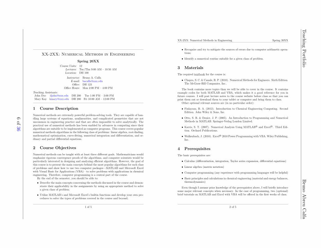
XX-2XX: Numerical Methods in EngineeringSpring 20XX

Course Units: 12Lectures: Tue/Thu 9:00 AM – 10:50 AMLocation: DH 100Instructor: Bruno A. Calfa

E-mail: [email protected]: DH 123

Office Hours: Mon 2:00 PM – 4:00 PMTeaching Assistants:John Doe [email protected] DH 200 Tue 1:00 PM – 3:00 PMMary Kay [email protected] DH 200 Fri 10:00 AM – 12:00 PM

1 Course DescriptionNumerical methods are extremely powerful problem-solving tools. They are capable of han-dling large systems of equations, nonlinearities, and complicated geometries that are notuncommon in engineering practice and that are often impossible to solve analytically. Thepractical use of numerical methods has been enabled by advances in computing since theiralgorithms are suitable to be implemented as computer programs. This course covers popularnumerical methods algorithms in the following class of problems: linear algebra, root-finding,mathematical optimization, curve-fitting, numerical integration and differentiation, and or-dinary and partial differential equations.

2 Course ObjectivesNumerical methods can be taught with at least three different goals. Mathematicians wouldemphasize rigorous convergence proofs of the algorithms, and computer scientists would beparticularly interested in designing and analyzing efficient algorithms. However, the goal ofthis course is to present the main concepts behind the most popular algorithms for each classof problems and show how to use two computer packages—MATLAB and Microsoft Excelwith Visual Basic for Applications (VBA)—to solve problems with applications in chemicalengineering. Therefore, computer programming is a central part of the course.

By the end of the semester, you should be able to:• Describe the main concepts concerning the methods discussed in the course and demon-

strate their applicability in the assignments by using an appropriate method to solvea given class of problem;

• Utilize MATLAB’s and Microsoft Excel’s builtin functions and develop your own pro-cedures to solve the types of problems covered in the course and beyond;

1 of 5

XX-2XX: Numerical Methods in Engineering Spring 20XX

• Recognize and try to mitigate the sources of errors due to computer arithmetic opera-tions;

• Identify a numerical routine suitable for a given class of problem.

3 MaterialsThe required textbook for the course is:

• Chapra, S. C. & Canale, R. P. (2010). Numerical Methods for Engineers. Sixth Edition.The McGraw-Hill Companies, Inc..

The book contains more topics than we will be able to cover in the course. It containsexample codes for both MATLAB and VBA, which makes it a good reference for you infuture courses. I will post lecture notes to the course website before class so that you canprint them out or download them to your tablet or computer and bring them to class.

Other optional relevant sources are (in no particular order):

• Finlayson, B. A. (2012). Introduction to Chemical Engineering Computing. SecondEdition. John Wiley & Sons, Inc.

• Otto, S. R. & Denier, J. P. (2005). An Introduction to Programming and NumericalMethods in MATLAB. Springer-Verlag London Limited.

• Karris, S. T. (2007). Numerical Analysis Using MATLAB R© and Excel R©. Third Edi-tion. Orchard Publications.

• Walkenbach, J. (2010). Excel R© 2010 Power Programming with VBA. Wiley Publishing,Inc.

4 PrerequisitesThe basic prerequisites are:

• Calculus (differentiation, integration, Taylor series expansion, differential equations)

• Linear algebra (matrix notation)

• Computer programming (any experience with programming languages will be helpful)

• Basic principles and calculations in chemical engineering (material and energy balances,thermodynamics)

Even though I assume prior knowledge of the prerequisites above, I will briefly introducesome major relevant concepts when necessary. In the case of programming, two (optional)brief tutorials on MATLAB and Excel with VBA will be offered in the first weeks of class.

2 of 5

TeachingPortfolio

Bruno

Abreu

Calfa

6of36


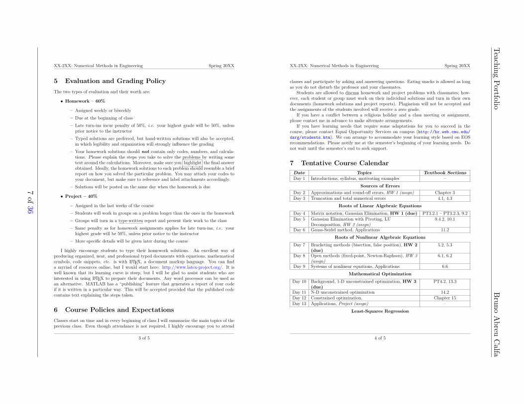
5 Evaluation and Grading PolicyThe two types of evaluation and their worth are:

• Homework – 60%

– Assigned weekly or biweekly– Due at the beginning of class– Late turn-ins incur penalty of 50%, i.e. your highest grade will be 50%, unless

prior notice to the instructor– Typed solutions are preferred, but hand-written solutions will also be accepted,

in which legibility and organization will strongly influence the grading– Your homework solutions should not contain only codes, numbers, and calcula-

tions. Please explain the steps you take to solve the problems by writing sometext around the calculations. Moreover, make sure you highlight the final answerobtained. Ideally, the homework solutions to each problem should resemble a briefreport on how you solved the particular problem. You may attach your codes toyour document, but make sure to reference and label attachments accordingly.

– Solutions will be posted on the same day when the homework is due

• Project – 40%

– Assigned in the last weeks of the course– Students will work in groups on a problem longer than the ones in the homework– Groups will turn in a type-written report and present their work to the class– Same penalty as for homework assignments applies for late turn-ins, i.e. your

highest grade will be 50%, unless prior notice to the instructor– More specific details will be given later during the course

I highly encourage students to type their homework solutions. An excellent way ofproducing organized, neat, and professional typed documents with equations, mathematicalsymbols, code snippets, etc. is with LATEX, a document markup language. You can finda myriad of resources online, but I would start here: http://www.latex-project.org/. It iswell known that its learning curve is steep, but I will be glad to assist students who areinterested in using LATEX to prepare their documents. Any word processor can be used asan alternative. MATLAB has a “publishing” feature that generates a report of your codeif it is written in a particular way. This will be accepted provided that the published codecontains text explaining the steps taken.

6 Course Policies and ExpectationsClasses start on time and in every beginning of class I will summarize the main topics of theprevious class. Even though attendance is not required, I highly encourage you to attend

3 of 5


classes and participate by asking and answering questions. Eating snacks is allowed as longas you do not disturb the professor and your classmates.

Students are allowed to discuss homework and project problems with classmates; how-ever, each student or group must work on their individual solutions and turn in their owndocuments (homework solutions and project reports). Plagiarism will not be accepted andthe assignments of the students involved will receive a zero grade.

If you have a conflict between a religious holiday and a class meeting or assignment,please contact me in advance to make alternate arrangements.

If you have learning needs that require some adaptations for you to succeed in thecourse, please contact Equal Opportunity Services on campus (http://hr.web.cmu.edu/dsrg/students.htm). We can arrange to accommodate your learning style based on EOSrecommendations. Please notify me at the semester’s beginning of your learning needs. Donot wait until the semester’s end to seek support.

7 Tentative Course CalendarDate Topics Textbook SectionsDay 1 Introductions, syllabus, motivating examples –

Sources of ErrorsDay 2 Approximations and round-off errors, HW 1 (assgn) Chapter 3Day 3 Truncation and total numerical errors 4.1, 4.3

Roots of Linear Algebraic EquationsDay 4 Matrix notation, Gaussian Elimination, HW 1 (due) PT3.2.1 – PT3.2.3, 9.2Day 5 Gaussian Elimination with Pivoting, LU

Decomposition, HW 2 (assgn)9.4.2, 10.1

Day 6 Gauss-Seidel method, Applications 11.2Roots of Nonlinear Algebraic Equations

Day 7 Bracketing methods (bisection, false position), HW 2(due)

5.2, 5.3

Day 8 Open methods (fixed-point, Newton-Raphson), HW 3(assgn)

6.1, 6.2

Day 9 Systems of nonlinear equations, Applications 6.6Mathematical Optimization

Day 10 Background, 1-D unconstrained optimization, HW 3(due)

PT4.2, 13.3

Day 11 N-D unconstrained optimization 14.2Day 12 Constrained optimization, Chapter 15Day 13 Applications, Project (assgn) –

Least-Squares Regression

4 of 5

TeachingPortfolio

Bruno

Abreu

Calfa

7of36


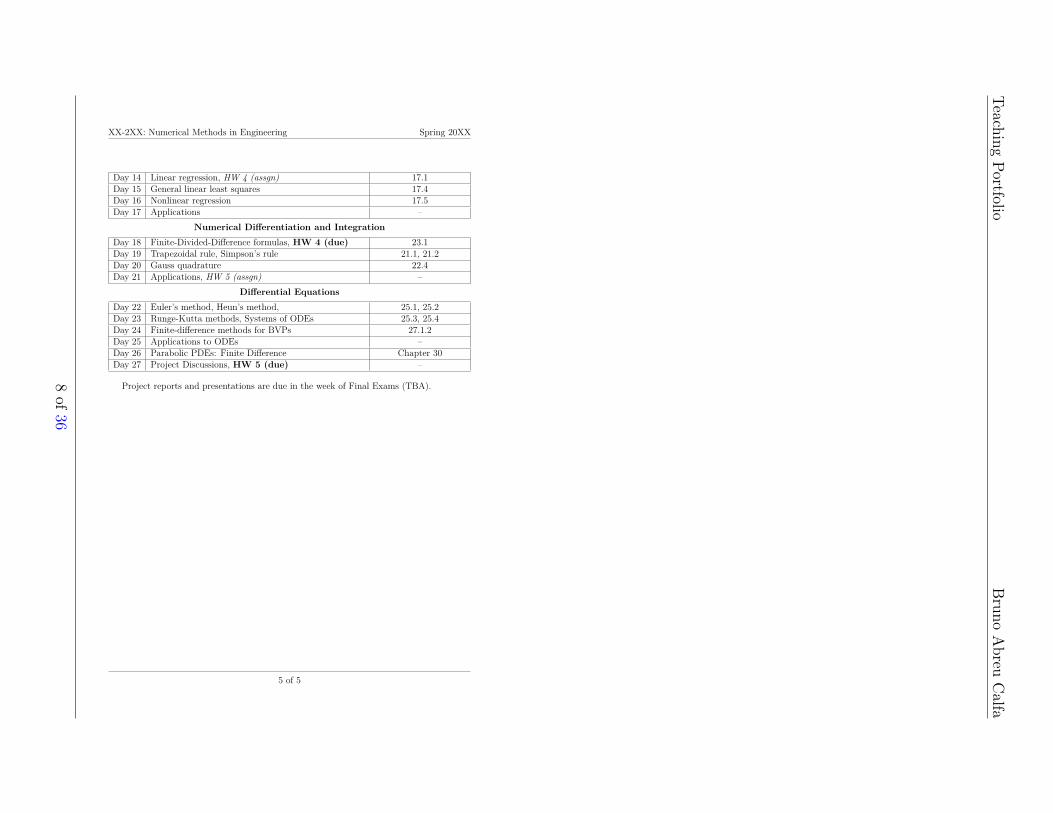
Day 14 Linear regression, HW 4 (assgn) 17.1Day 15 General linear least squares 17.4Day 16 Nonlinear regression 17.5Day 17 Applications –

Numerical Differentiation and IntegrationDay 18 Finite-Divided-Difference formulas, HW 4 (due) 23.1Day 19 Trapezoidal rule, Simpson’s rule 21.1, 21.2Day 20 Gauss quadrature 22.4Day 21 Applications, HW 5 (assgn) –

Differential EquationsDay 22 Euler’s method, Heun’s method, 25.1, 25.2Day 23 Runge-Kutta methods, Systems of ODEs 25.3, 25.4Day 24 Finite-difference methods for BVPs 27.1.2Day 25 Applications to ODEs –Day 26 Parabolic PDEs: Finite Difference Chapter 30Day 27 Project Discussions, HW 5 (due) –

Project reports and presentations are due in the week of Final Exams (TBA).

5 of 5

TeachingPortfolio

Bruno

Abreu

Calfa

8of36


Appendix B MATLAB Tutorial: Fall 2011This appendix contains the MATLAB tutorial material I prepared and presented to un-dergraduate students that ranged from sophomores to seniors. The two-part tutorial wasobserved by colleagues at the Eberly Center for Teaching Excellence at CMU, and was heldin two days, each with one-hour-and-half sessions.

For brevity, only the handout versions of the slides presented are shown in the followingpages. This updated version (Fall 2013) is slightly different from the one I used during thetutorial sessions in Fall 2011. It contains fixes to typographical errors and pictures of thewindows of the new MATLAB graphical user interface (2012 onward). In addition to theslides, I also prepared two sets of homework questions with solutions (not included) so thatstudents could practice what was covered in the tutorial sessions. I held the tutorial sessionsin two days, and each session lasted for one hour and fifty minutes.

This two-part tutorial assumes no previous familiarity with MATLAB as it starts with“opening MATLAB” and the main windows students should focus on specially in the be-ginning. While presenting the material, I alternate between the slides and MATLAB forpractical demonstrations. I also allow students time to practice themselves. I purposely in-clude logical errors in the MATLAB examples to show the students how the software handlesuser errors. I show the students how to use the error message issued by MATLAB to guidethem on how to fix the error. In every topic, after showing some examples with solutions,I ask students to provide solutions to other examples slightly more demanding in order togauge their understanding. Finally, before starting a new topic, for example “2-D Arrays”, Ibriefly summarize the main concepts of the immediate relevant topics, for example “ScalarVariables” and “1-D Arrays”.

9 of 36

MATLAB: IntroductionPart 1

Bruno Abreu Calfa

Last Update: September 16, 2013

Table of ContentsOutline

Contents1 What is MATLAB? 1

2 MATLAB Windows 2

3 MATLAB as a Calculator 3

4 MATLAB Classes 3

5 Scripts and Functions 65.1 Writing MATLAB Programs . . . . . . . . . . . . . . . . . . . . . . . . . . . . . . . . . . . . . . . 65.2 Code Cells and Publishing . . . . . . . . . . . . . . . . . . . . . . . . . . . . . . . . . . . . . . . . 6

1 What is MATLAB?A powerful tool!

• MATLAB stands for Matrix Laboratory

• Enhanced by toolboxes (specific routines for an area of application)

– Optimization

– Statistics

– Control System

– Bioinformatics

– . . .

• Excellent for numerical computations

• Commonly regarded as a ‘Rapid Prototyping Tool’

• Used in industry and academia

1

Help with MATLAB?

• MATLAB’s Help

• Google

• A book about MATLAB

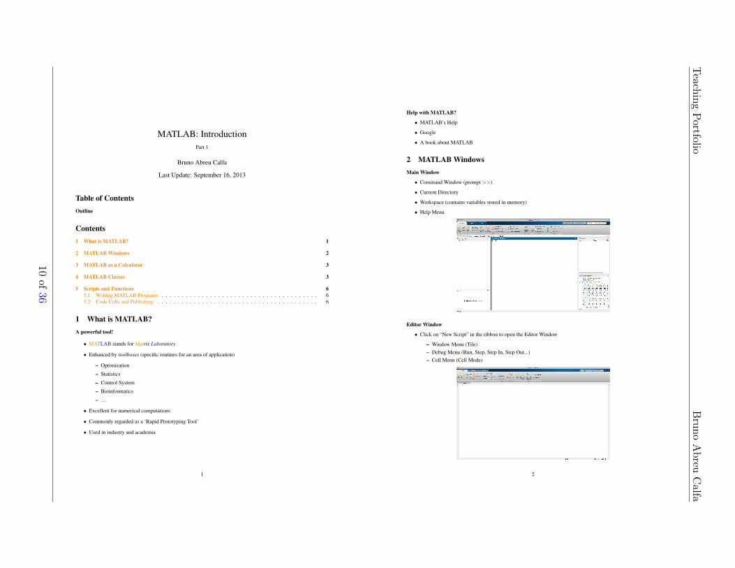
2 MATLAB WindowsMain Window

• Command Window (prompt >>)

• Current Directory

• Workspace (contains variables stored in memory)

• Help Menu

Editor Window

• Click on “New Script” in the ribbon to open the Editor Window

– Window Menu (Tile)– Debug Menu (Run, Step, Step In, Step Out...)– Cell Menu (Cell Mode)

2

TeachingPortfolio

Bruno

Abreu

Calfa

10of36

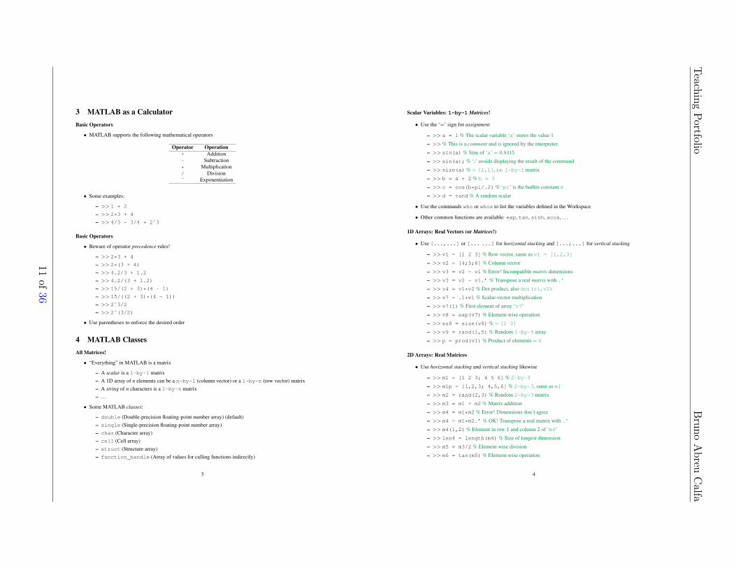
3 MATLAB as a CalculatorBasic Operators

• MATLAB supports the following mathematical operators

Operator Operation+ Addition- Subtraction* Multiplication/ Divisionˆ Exponentiation

• Some examples:

– >> 1 + 2

– >> 2*3 + 4

– >> 4/3 - 3/4 + 2ˆ3

Basic Operators

• Beware of operator precedence rules!

– >> 2*3 + 4

– >> 2*(3 + 4)

– >> 4.2/3 + 1.2

– >> 4.2/(3 + 1.2)

– >> 15/(2 + 3)*(4 - 1)

– >> 15/((2 + 3)*(4 - 1))

– >> 2ˆ3/2

– >> 2ˆ(3/2)

• Use parentheses to enforce the desired order

4 MATLAB ClassesAll Matrices!

• “Everything” in MATLAB is a matrix

– A scalar is a 1-by-1 matrix– A 1D array of n elements can be a n-by-1 (column vector) or a 1-by-n (row vector) matrix– A string of n characters is a 1-by-n matrix– . . .

• Some MATLAB classes:

– double (Double-precision floating-point number array) (default)– single (Single-precision floating-point number array)– char (Character array)– cell (Cell array)– struct (Structure array)– function_handle (Array of values for calling functions indirectly)

3

Scalar Variables: 1-by-1 Matrices!

• Use the ‘=’ sign for assignment

– >> a = 1 % The scalar variable ‘a’ stores the value 1

– >> % This is a comment and is ignored by the interpreter

– >> sin(a) % Sine of ‘a’ = 0.8415

– >> sin(a); % ‘;’ avoids displaying the result of the command

– >> size(a) % = [1,1], i.e. 1-by-1 matrix

– >> b = a + 2 % b = 3

– >> c = cos(b*pi/.2) % ‘pi’ is the builtin constant ⇡

– >> d = rand % A random scalar

• Use the commands who or whos to list the variables defined in the Workspace

• Other common functions are available: exp, tan, sinh, acos, . . .

1D Arrays: Real Vectors (or Matrices!)

• Use [...,...] or [... ...] for horizontal stacking and [...;...] for vertical stacking

– >> v1 = [1 2 3] % Row vector, same as v1 = [1,2,3]

– >> v2 = [4;5;6] % Column vector

– >> v3 = v2 - v1 % Error! Incompatible matrix dimensions

– >> v3 = v2 - v1.’ % Transpose a real matrix with .’

– >> v4 = v1*v2 % Dot product, also dot(v1,v2)

– >> v7 = .1*v1 % Scalar-vector multiplication

– >> v7(1) % First element of array ‘v7’

– >> v8 = exp(v7) % Element-wise operation

– >> sz8 = size(v8) % = [1 3]

– >> v9 = rand(1,5) % Random 1-by-5 array

– >> p = prod(v1) % Product of elements = 6

2D Arrays: Real Matrices

• Use horizontal stacking and vertical stacking likewise

– >> m1 = [1 2 3; 4 5 6] % 2-by-3

– >> m1p = [1,2,3; 4,5,6] % 2-by-3, same as m1

– >> m2 = rand(2,3) % Random 2-by-3 matrix

– >> m3 = m1 + m2 % Matrix addition

– >> m4 = m1*m2 % Error! Dimensions don’t agree

– >> m4 = m1*m2.’ % OK! Transpose a real matrix with .’

– >> m4(1,2) % Element in row 1 and column 2 of ‘m4’

– >> len4 = length(m4) % Size of longest dimension

– >> m5 = m3/2 % Element-wise division

– >> m6 = tan(m5) % Element-wise operation

4

TeachingPortfolio

Bruno

Abreu

Calfa

11of36

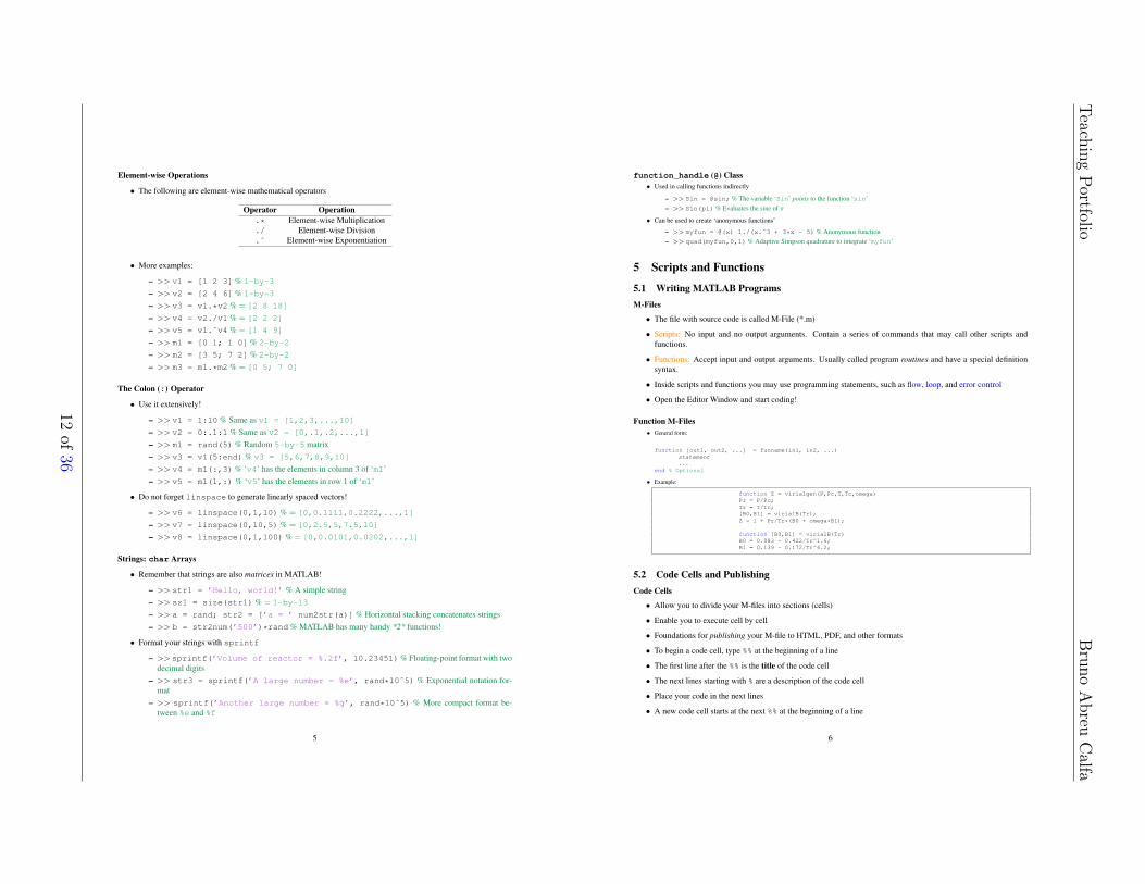
Element-wise Operations

• The following are element-wise mathematical operators

Operator Operation.* Element-wise Multiplication./ Element-wise Division.ˆ Element-wise Exponentiation

• More examples:

– >> v1 = [1 2 3] % 1-by-3

– >> v2 = [2 4 6] % 1-by-3

– >> v3 = v1.*v2 % = [2 8 18]

– >> v4 = v2./v1 % = [2 2 2]

– >> v5 = v1.ˆv4 % = [1 4 9]

– >> m1 = [0 1; 1 0] % 2-by-2

– >> m2 = [3 5; 7 2] % 2-by-2

– >> m3 = m1.*m2 % = [0 5; 7 0]

The Colon (:) Operator

• Use it extensively!

– >> v1 = 1:10 % Same as v1 = [1,2,3,...,10]

– >> v2 = 0:.1:1 % Same as v2 = [0,.1,.2,...,1]

– >> m1 = rand(5) % Random 5-by-5 matrix– >> v3 = v1(5:end) % v3 = [5,6,7,8,9,10]

– >> v4 = m1(:,3) % ‘v4’ has the elements in column 3 of ‘m1’– >> v5 = m1(1,:) % ‘v5’ has the elements in row 1 of ‘m1’

• Do not forget linspace to generate linearly spaced vectors!

– >> v6 = linspace(0,1,10) % = [0,0.1111,0.2222,...,1]

– >> v7 = linspace(0,10,5) % = [0,2.5,5,7.5,10]

– >> v8 = linspace(0,1,100) % = [0,0.0101,0.0202,...,1]

Strings: char Arrays

• Remember that strings are also matrices in MATLAB!

– >> str1 = ’Hello, world!’ % A simple string– >> sz1 = size(str1) % = 1-by-13

– >> a = rand; str2 = [’a = ’ num2str(a)] % Horizontal stacking concatenates strings– >> b = str2num(’500’)*rand % MATLAB has many handy *2* functions!

• Format your strings with sprintf

– >> sprintf(’Volume of reactor = %.2f’, 10.23451)% Floating-point format with twodecimal digits

– >> str3 = sprintf(’A large number = %e’, rand*10ˆ5) % Exponential notation for-mat

– >> sprintf(’Another large number = %g’, rand*10ˆ5) % More compact format be-tween %e and %f

5

function_handle (@) Class• Used in calling functions indirectly

– >> Sin = @sin; % The variable ‘Sin’ points to the function ‘sin’– >> Sin(pi) % Evaluates the sine of ⇡

• Can be used to create ‘anonymous functions’

– >> myfun = @(x) 1./(x.ˆ3 + 3*x - 5) % Anonymous function– >> quad(myfun,0,1) % Adaptive Simpson quadrature to integrate ‘myfun’

5 Scripts and Functions

5.1 Writing MATLAB ProgramsM-Files

• The file with source code is called M-File (*.m)

• Scripts: No input and no output arguments. Contain a series of commands that may call other scripts andfunctions.

• Functions: Accept input and output arguments. Usually called program routines and have a special definitionsyntax.

• Inside scripts and functions you may use programming statements, such as flow, loop, and error control

• Open the Editor Window and start coding!

Function M-Files• General form:

function [out1, out2, ...] = funname(in1, in2, ...)statement...

end % Optional

• Example:

function Z = virialgen(P,Pc,T,Tc,omega)Pr = P/Pc;Tr = T/Tc;[B0,B1] = virialB(Tr);Z = 1 + Pr/Tr*(B0 + omega*B1);

function [B0,B1] = virialB(Tr)B0 = 0.083 - 0.422/Tr^1.6;B1 = 0.139 - 0.172/Tr^4.2;

5.2 Code Cells and PublishingCode Cells

• Allow you to divide your M-files into sections (cells)

• Enable you to execute cell by cell

• Foundations for publishing your M-file to HTML, PDF, and other formats

• To begin a code cell, type %% at the beginning of a line

• The first line after the %% is the title of the code cell

• The next lines starting with % are a description of the code cell

• Place your code in the next lines

• A new code cell starts at the next %% at the beginning of a line

6

TeachingPortfolio

Bruno

Abreu

Calfa

12of36

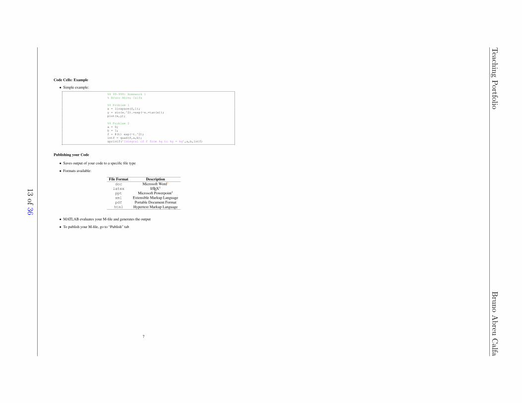
Code Cells: Example

• Simple example:

%% 99-999: Homework 1% Bruno Abreu Calfa

%% Problem 1x = linspace(0,1);y = sin(x.^2).*exp(-x.*tan(x));plot(x,y);

%% Problem 2a = 0;b = 1;f = @(t) exp(-t.^2);intf = quad(f,a,b);sprintf(’Integral of f from %g to %g = %g’,a,b,intf)

Publishing your Code

• Saves output of your code to a specific file type

• Formats available:

File Format Descriptiondoc Microsoft Word1

latex LATEX1

ppt Microsoft Powerpoint1

xml Extensible Markup Languagepdf Portable Document Formathtml Hypertext Markup Language

• MATLAB evaluates your M-file and generates the output

• To publish your M-file, go to “Publish” tab

7

TeachingPortfolio

Bruno

Abreu

Calfa

13of36

MATLAB: IntroductionPart 2

Bruno Abreu Calfa

Last Update: September 16, 2013

Table of ContentsOutline

Contents1 MATLAB Classes 1

2 Elements of Programming 2

3 Plotting 43.1 2-D Plotting . . . . . . . . . . . . . . . . . . . . . . . . . . . . . . . . . . . . . . . . . . . . . . . . 43.2 3-D Plotting . . . . . . . . . . . . . . . . . . . . . . . . . . . . . . . . . . . . . . . . . . . . . . . . 6

1 MATLAB ClassesND Arrays

• MATLAB allows multidimensional arrays (n dimensions)

– >> nd1 = zeros(2,3,4) % 2-by-3-by-4 full of 0s

– >> nd2 = ones(10,5,8,7) % 10-by-5-by-8-by-7 full of 1s

– >> nd1(:,1,2) = 1:2 % Replaces column 1 of page 2 by [1,2]

– >> nd2(:,:,5,7) = rand(10,5) % Replaces rows and columns of page 5 and chapter 7 by ran-dom 10-by-5 matrix

Cell and Structure Arrays

• Cell Arrays (cell): generic containers (store any type of data)

– >> cell1 = {’aaa’, 1, rand(2,3)} % Use curly braces to retrieve/assign values

– >> a = cell1(1) % ‘a’ is the first container (also a cell)

– >> b = cell1{1} % ‘b’ is the first content (a char array)

– >> cell1{:} % {:} generates a comma-separated list

– >> [a,b,c] = cell1{:} % Assigns each content to a variable

• Structure Arrays (struct): data types with fields and values

– >> methane.omega = .012; % Methane’s acentric factor

– >> methane.Tc = 190.6; % Its critical temperature, K

– >> methane.Pc = 45.99; % Its critical pressure, bar

– >> methane % Display methane fields and values

1

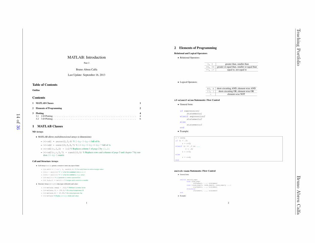
2 Elements of ProgrammingRelational and Logical Operators

• Relational Operators:

>, < greater than, smaller than>=, <= greater or equal than, smaller or equal than==, ⇠= equal to, not equal to

• Logical Operators:

&&, & short-circuiting AND, element-wise AND||, | short-circuiting OR, element-wise OR

⇠ element-wise NOT

if-elseif-else Statements: Flow Control

• General form:

if expression1statements1

elseif expression2statements2

elsestatements3

end

• Example:

r = rand;

if (r < .3)

r = r*2;

elseif (r >= .3 && ...

r < .6)

r = r*3;

else

r = r*4;

end

switch-case Statements: Flow Control• General form:

switch switch_exprcase case_expr

statement, ..., statementcase {case_expr1, case_expr2, case_expr3, ...}

statement, ..., statementotherwise

statement, ..., statementend

• Example:

2

TeachingPortfolio

Bruno

Abreu

Calfa

14of36

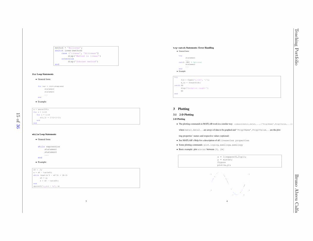
method = ’Bilinear’;switch lower(method)

case {’linear’, ’bilinear’}disp(’Method is linear’)

otherwisedisp(’Unknown method’)

end

for Loop Statements

• General form:

for var = init:step:end

statement

statement

...

end

• Example:

a = zeros(10);

for i = 1:10

for j = 1:10

a(i,j) = 1/(i+j-1);

end

end

while Loop Statements

• General form:

while expressionstatementstatement...

end

• Example:

x0 = .5;

x = x0 - tan(x0);

while (sqrt(xˆ2 - x0ˆ2) > 1E-3)

x0 = x;

x = x0 - tan(x0);

end

sprintf(’x_end = %g’, x)

3

try-catch Statements: Error Handling• General form:

trystatement...

catch [ME] % Optionalstatement...

end

• Example:

try

fid = fopen(’a.txt’, ’r’);

d_in = fread(fid);

catch EX

disp(’Exception caught!’)

EX

end

3 Plotting

3.1 2-D Plotting2-D Plotting

• The plotting commands in MATLAB work in a similar way: command(data1,data2,...,[’Prop1Name’,Prop1Value,...])

where data1, data2, . . . are arrays of data to be graphed and ’Prop1Name’, Prop1Value, . . . are the plot-

ting properties’ names and respective values (optional)

• See MATLAB’s Help for a description of all lineseries properties

• Some plotting commands: plot, loglog, semilogx, semilogy

• Basic example: plot sin(x) between [0, 2⇡]

x = linspace(0,2*pi);y = sin(x);figureplot(x,y);

4

TeachingPortfolio

Bruno

Abreu

Calfa

15of36

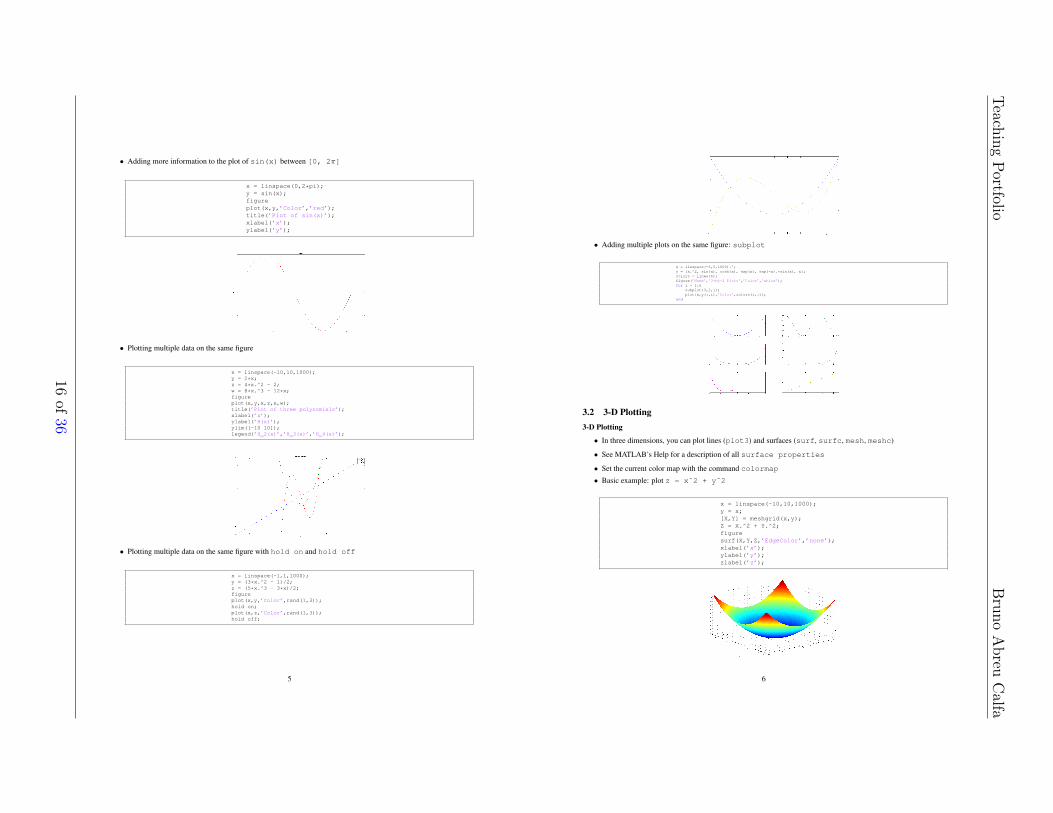
• Adding more information to the plot of sin(x) between [0, 2⇡]

x = linspace(0,2*pi);y = sin(x);figureplot(x,y,’Color’,’red’);title(’Plot of sin(x)’);xlabel(’x’);ylabel(’y’);

• Plotting multiple data on the same figure

x = linspace(-10,10,1000);y = 2*x;z = 4*x.^2 - 2;w = 8*x.^3 - 12*x;figureplot(x,y,x,z,x,w);title(’Plot of three polynomials’);xlabel(’x’);ylabel(’H(x)’);ylim([-10 10]);legend(’H_2(x)’,’H_3(x)’,’H_4(x)’);

• Plotting multiple data on the same figure with hold on and hold off

x = linspace(-1,1,1000);y = (3*x.^2 - 1)/2;z = (5*x.^3 - 3*x)/2;figureplot(x,y,’Color’,rand(1,3));hold on;plot(x,z,’Color’,rand(1,3));hold off;

5

• Adding multiple plots on the same figure: subplot

x = linspace(-5,5,1000).’;y = [x.^2, sin(x), cosh(x), exp(x), exp(-x).*sin(x), x];colors = lines(6);figure(’Name’,’3-by-2 Plots’,’Color’,’white’);for i = 1:6

subplot(3,2,i);plot(x,y(:,i),’Color’,colors(i,:));

end

3.2 3-D Plotting3-D Plotting

• In three dimensions, you can plot lines (plot3) and surfaces (surf, surfc, mesh, meshc)

• See MATLAB’s Help for a description of all surface properties

• Set the current color map with the command colormap

• Basic example: plot z = xˆ2 + yˆ2

x = linspace(-10,10,1000);y = x;[X,Y] = meshgrid(x,y);Z = X.^2 + Y.^2;figuresurf(X,Y,Z,’EdgeColor’,’none’);xlabel(’x’);ylabel(’y’);zlabel(’z’);

6

TeachingPortfolio

Bruno

Abreu

Calfa

16of36

• Adding contours to z = xˆ2 - yˆ2

x = linspace(-5,5,50);y = x;[X,Y] = meshgrid(x,y);Z = X.^2 - Y.^2;figurecolormap(’cool’);meshc(X,Y,Z);xlabel(’x’);ylabel(’y’);zlabel(’z’);

7

TeachingPortfolio

Bruno

Abreu

Calfa

17of36


Appendix C Guest Lectures on Climate Change: Fall2013

This appendix contains the slides I prepared under the supervision of a subject-matter experton climate change (Prof. Neil Donahue), and used during two lectures in the Introduction toChemical Engineering freshman course. The two guest lectures were observed by colleaguesat the Eberly Center at CMU, and were held in two days, each with fifty-minute longsessions. In addition to the slides, I also prepared two homework questions with solutions (notincluded), in which students were asked to perform basic calculations and use of MATLABto practice the concepts discussed in the two lectures. I gave the lectures in two days, andeach lecture lasted for fifty minutes.

The first set of slides (Part I) contains several graphics to illustrate the effects of green-house gases in the climate. The visuals also served the purpose of illustrating key conceptsin climatology. In addition to pointing students to official websites about climate change,I made use of readily available online video clips to complement the material in the slides.The second set of slides (Part II) contains more of the mechanics of problem-solving in thecontext of climate change. It makes connections with topics covered in the course, such asconcentrations, proportions, and the Ideal Gas Law. In addition, I explained how MATLABcan be used to solve the numerical examples in the slides.

18 of 36

06-‐100: Introduc/on to Chemical Engineering

Climate and CO2 -‐ Part I

September 23rd, 2013

Bruno Calfa Prof. Kris Dahl

1

Outline

•  Introduc/on to Climate Change – Defini/ons – Primary cause – Radia/ve Balance

•  [CO2] and Earth’s Temperature •  Anthropogenic CO2 Emissions – Fossil Fuel Combus/on

2

TeachingPortfolio

Bruno

Abreu

Calfa

19of36

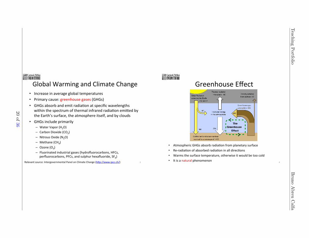
Global Warming and Climate Change •  Increase in average global temperatures •  Primary cause: greenhouse gases (GHGs) •  GHGs absorb and emit radia/on at specific wavelengths

within the spectrum of thermal infrared radia/on emiWed by the Earth’s surface, the atmosphere itself, and by clouds

•  GHGs include primarily –  Water Vapor (H2O) –  Carbon Dioxide (CO2) –  Nitrous Oxide (N2O) –  Methane (CH4) –  Ozone (O3) –  Fluorinated industrial gases (hydrofluorocarbons, HFCs,

perfluorocarbons, PFCs, and sulphur hexafluoride, SF6) 3 Relevant source: Intergovernmental Panel on Climate Change (hWp://www.ipcc.ch/)

Greenhouse Effect

•  Atmospheric GHGs absorb radia/on from planetary surface •  Re-‐radia/on of absorbed radia/on in all direc/ons •  Warms the surface temperature, otherwise it would be too cold •  It is a natural phenomenon 4

TeachingPortfolio

Bruno

Abreu

Calfa

20of36

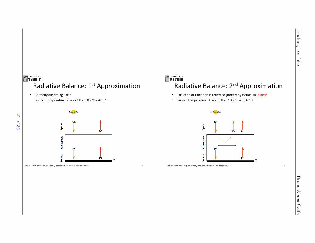
Radia/ve Balance: 1st Approxima/on •  Perfectly absorbing Earth •  Surface temperature: Ts = 279 K = 5.85 oC = 42.5 oF

5 Values in W m−2. Figure kindly provided by Prof. Neil Donahue.

Ts

Radia/ve Balance: 2nd Approxima/on •  Part of solar radia/on is reflected (mostly by clouds) => albedo •  Surface temperature: Ts = 255 K = −18.2 oC = −0.67 oF


Ts

TeachingPortfolio

Bruno

Abreu

Calfa

21of36

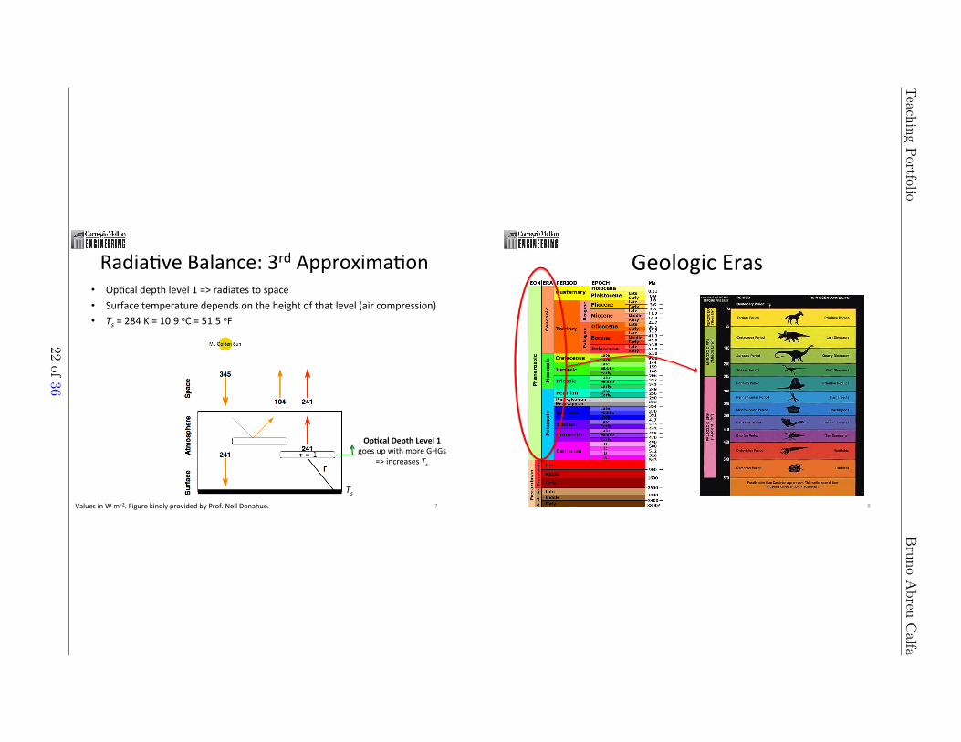
Radia/ve Balance: 3rd Approxima/on •  Op/cal depth level 1 => radiates to space •  Surface temperature depends on the height of that level (air compression) •  Ts = 284 K = 10.9 oC = 51.5 oF


Op#cal Depth Level 1 goes up with more GHGs

=> increases Ts

Ts

Geologic Eras

8

TeachingPortfolio

Bruno

Abreu

Calfa

22of36

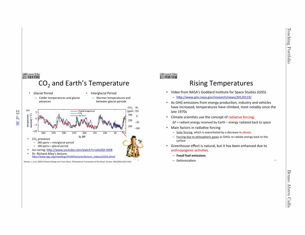
CO2 and Earth’s Temperature •  Glacial Period

–  Colder temperatures and glacier advances

•  Interglacial Period –  Warmer temperatures and

between glacial periods

9

•  CO2 presence –  280 ppmv = interglacial period –  180 ppmv = glacial period

•  Ice coring: hWp://www.youtube.com/watch?v=oHzADl-‐XID8 •  Dr. Richard Alley’s lecture:

hWp://www.agu.org/mee/ngs/fm09/lectures/lecture_videos/A23A.shtml

Hansen, J. et al. (2007) Climate Change and Trace Gases. Philosophical Transac/ons of the Royal. Society, 365(1856):1925-‐1924.

Rising Temperatures •  Video from NASA's Goddard Ins/tute for Space Studies (GISS)

–  hWp://www.giss.nasa.gov/research/news/20120119/ •  As GHG emissions from energy produc/on, industry and vehicles

have increased, temperatures have climbed, most notably since the late 1970s

•  Climate scien/sts use the concept of radia/ve forcing: ΔF = radiant energy received by Earth − energy radiated back to space

•  Main factors in radia/ve forcing –  Solar forcing, which is exacerbated by a decrease in albedo –  Forcing due to atmospheric gases as GHGs re-‐radiate energy back to the

surface •  Greenhouse effect is natural, but it has been enhanced due to

anthropogenic ac/vi/es –  Fossil fuel emissions –  Deforesta/on 10

TeachingPortfolio

Bruno

Abreu

Calfa

23of36

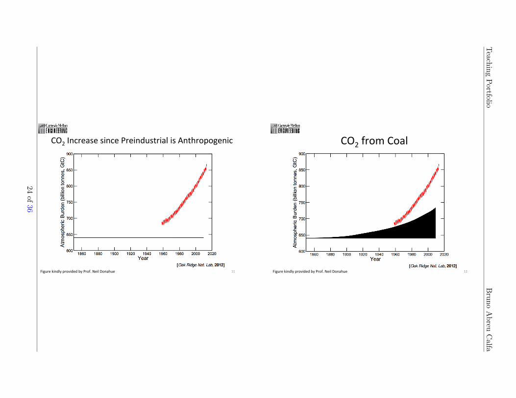
CO2 Increase since Preindustrial is Anthropogenic

11 Figure kindly provided by Prof. Neil Donahue

CO2 from Coal


TeachingPortfolio

Bruno

Abreu

Calfa

24of36

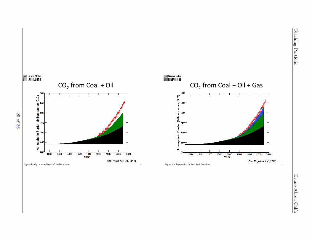
CO2 from Coal + Oil


CO2 from Coal + Oil + Gas


TeachingPortfolio

Bruno

Abreu

Calfa

25of36

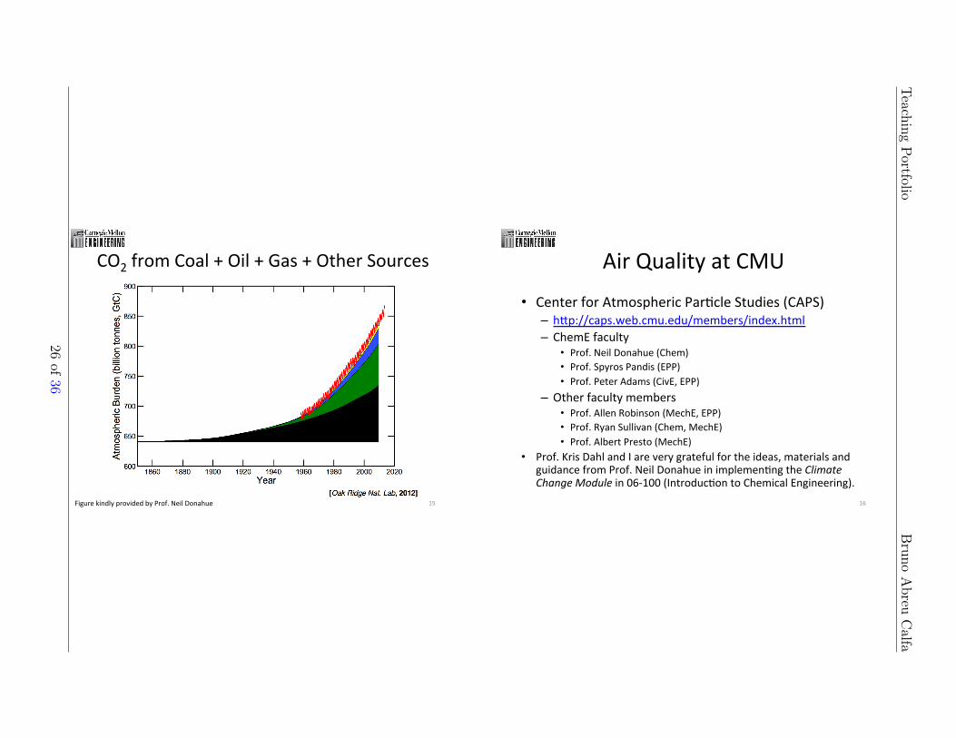
CO2 from Coal + Oil + Gas + Other Sources


Air Quality at CMU

•  Center for Atmospheric Par/cle Studies (CAPS) –  hWp://caps.web.cmu.edu/members/index.html –  ChemE faculty

•  Prof. Neil Donahue (Chem) •  Prof. Spyros Pandis (EPP) •  Prof. Peter Adams (CivE, EPP)

–  Other faculty members •  Prof. Allen Robinson (MechE, EPP) •  Prof. Ryan Sullivan (Chem, MechE) •  Prof. Albert Presto (MechE)

•  Prof. Kris Dahl and I are very grateful for the ideas, materials and guidance from Prof. Neil Donahue in implemen/ng the Climate Change Module in 06-‐100 (Introduc/on to Chemical Engineering).

16

TeachingPortfolio

Bruno

Abreu

Calfa

26of36

06-‐100: Introduc/on to Chemical Engineering

Climate and CO2 -‐ Part II

September 25th, 2013

Bruno Calfa Prof. Kris Dahl

1

Announcements •  Office Hours today

–  2:30 pm – 4:00 pm –  Cyert Hall B6A

•  Friday Lecture (09/27) –  Homework 4 and Recita/on 3 due: beginning of class – Majors Informa/on Session for Engineering Intro Courses

•  Recita/on 3 help material on Blackboard –  Help slides + Addi/onal informa/on on part (d)

•  ScoZ Ins/tute for Energy Innova/on –  hZp://www.cmu.edu/energy/ –  Energy Experts à By Topic Area

2

TeachingPortfolio

Bruno

Abreu

Calfa

27of36

Outline •  Quan/ta/ve Analysis –  Concentra/ons and frac/ons (emphasis on air) –  Ideal gas

•  Basic Calcula/ons – Molecular weight of dry air – Mass of C corresponding to 1 ppm of CO2 in the atmosphere (homework)

•  So`ware Workshop –  Reading and graphing pollu/on data in MATLAB –  Plot CO2 emissions in Mauna Loa (homework)

3

Concentra/ons and Frac/ons •  Mass-‐ or mole-‐based concentra/ons

•  In air, frac/ons are usually expressed on a molar or volume basis (equivalent for ideal gases)

also ppmv (on a volume basis), ppb, ppt… Example: 5 ppb of benzene in air means there are 5 × 10−9 moles of benzene in 1 mole of air

4

% 1 part species per 100 parts solu/on

ppm 1 part species per 106 parts solu/on

TeachingPortfolio

Bruno

Abreu

Calfa

28of36

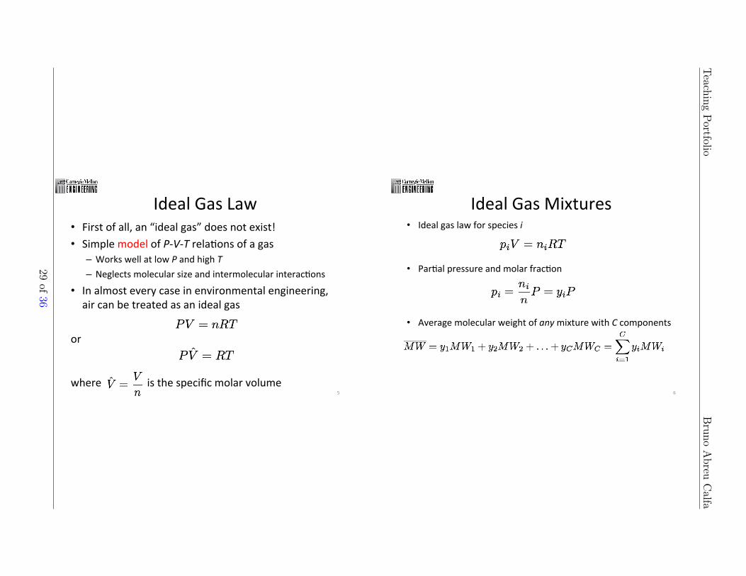
Ideal Gas Law •  First of all, an “ideal gas” does not exist! •  Simple model of P-‐V-‐T rela/ons of a gas

– Works well at low P and high T –  Neglects molecular size and intermolecular interac/ons

•  In almost every case in environmental engineering, air can be treated as an ideal gas

or

where is the specific molar volume 5

Ideal Gas Mixtures •  Ideal gas law for species i

•  Par/al pressure and molar frac/on

•  Average molecular weight of any mixture with C components

6

TeachingPortfolio

Bruno

Abreu

Calfa

29of36

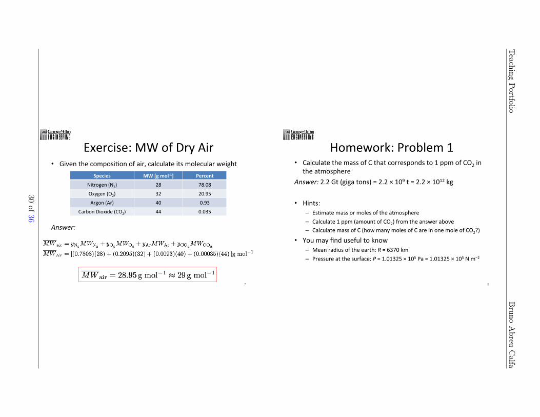
Exercise: MW of Dry Air •  Given the composi/on of air, calculate its molecular weight

Answer:

7

Species MW [g mol-‐1] Percent

Nitrogen (N2) 28 78.08

Oxygen (O2) 32 20.95

Argon (Ar) 40 0.93

Carbon Dioxide (CO2) 44 0.035

Homework: Problem 1 •  Calculate the mass of C that corresponds to 1 ppm of CO2 in

the atmosphere Answer: 2.2 Gt (giga tons) = 2.2 × 109 t = 2.2 × 1012 kg •  Hints:

–  Es/mate mass or moles of the atmosphere –  Calculate 1 ppm (amount of CO2) from the answer above –  Calculate mass of C (how many moles of C are in one mole of CO2?)

•  You may find useful to know –  Mean radius of the earth: R = 6370 km –  Pressure at the surface: P = 1.01325 × 105 Pa = 1.01325 × 105 N m−2

8

TeachingPortfolio

Bruno

Abreu

Calfa

30of36

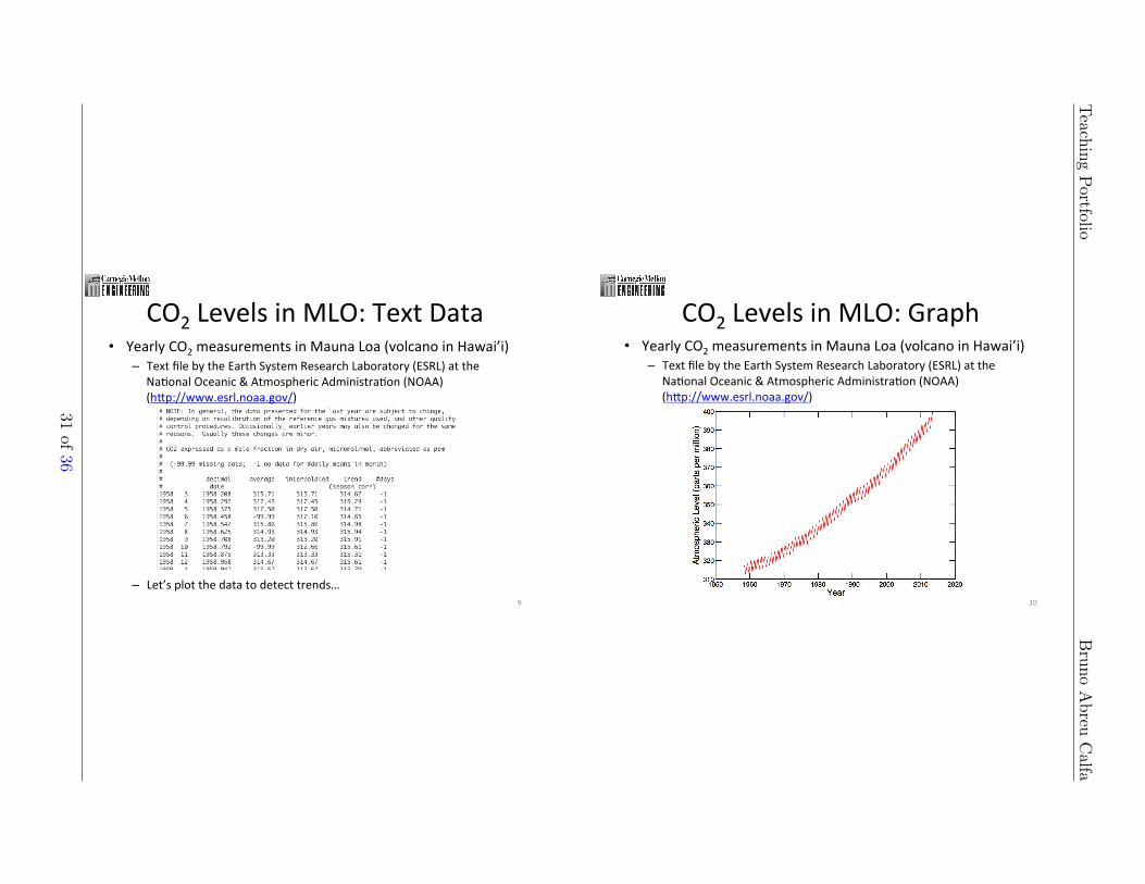
CO2 Levels in MLO: Text Data •  Yearly CO2 measurements in Mauna Loa (volcano in Hawai’i)

–  Text file by the Earth System Research Laboratory (ESRL) at the Na/onal Oceanic & Atmospheric Administra/on (NOAA) (hZp://www.esrl.noaa.gov/)

–  Let’s plot the data to detect trends… 9

CO2 Levels in MLO: Graph •  Yearly CO2 measurements in Mauna Loa (volcano in Hawai’i)

–  Text file by the Earth System Research Laboratory (ESRL) at the Na/onal Oceanic & Atmospheric Administra/on (NOAA) (hZp://www.esrl.noaa.gov/)

10

TeachingPortfolio

Bruno

Abreu

Calfa

31of36

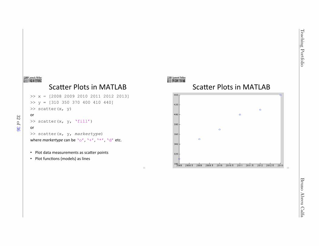
ScaZer Plots in MATLAB >> x = [2008 2009 2010 2011 2012 2013] >> y = [310 350 370 400 410 440]

>> scatter(x, y) or >> scatter(x, y, ‘fill’)

or >> scatter(x, y, markertype)

where markertype can be ‘o’, ‘+’, ‘*’, ‘d’ etc. •  Plot data measurements as scaZer points •  Plot func/ons (models) as lines

11

ScaZer Plots in MATLAB

12

TeachingPortfolio

Bruno

Abreu

Calfa

32of36

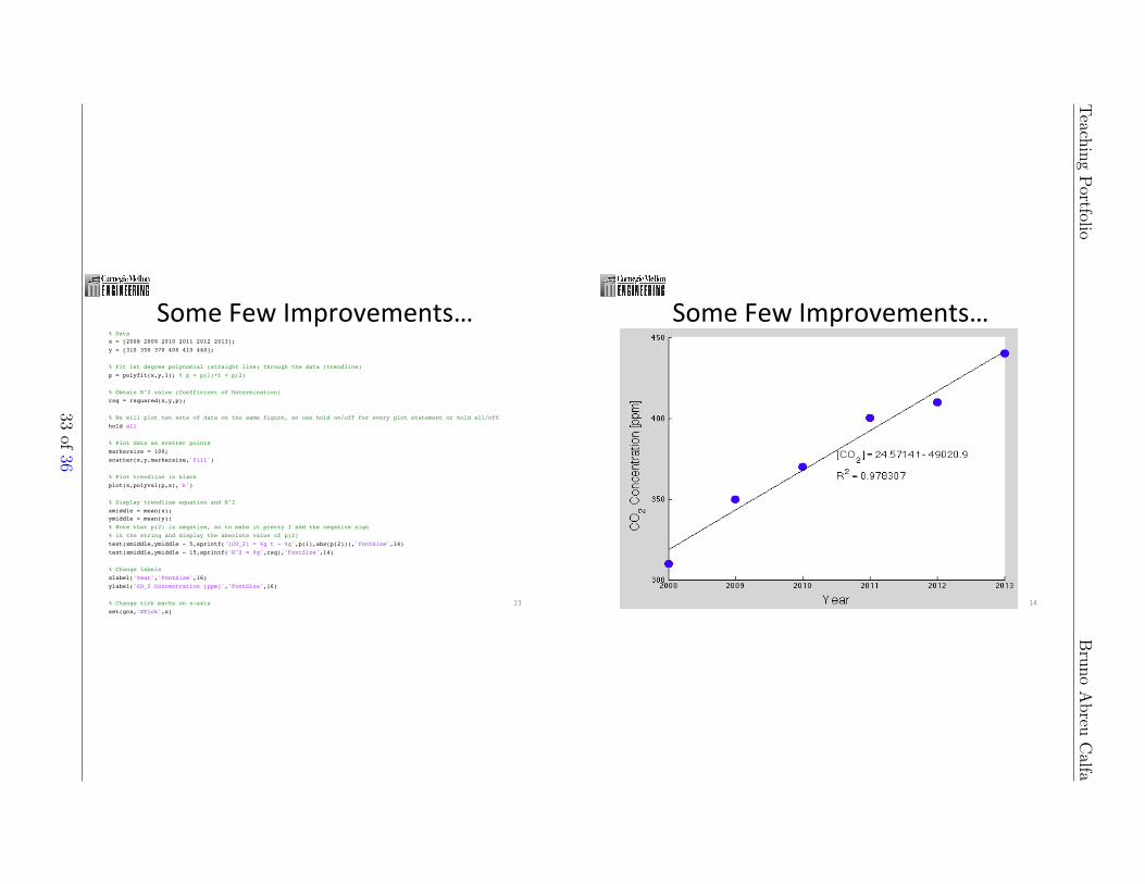
Some Few Improvements… % Data!x = [2008 2009 2010 2011 2012 2013];!y = [310 350 370 400 410 440];! !% Fit 1st degree polynomial (straight line) through the data (trendline)!p = polyfit(x,y,1); % p = p(1)*t + p(2)! !% Obtain R^2 value (Coefficient of Determination)!rsq = rsquared(x,y,p);! !% We will plot two sets of data on the same figure, so use hold on/off for every plot statement or hold all/off!hold all! !% Plot data as scatter points!markersize = 100;!scatter(x,y,markersize,'fill')! !% Plot trendline in black!plot(x,polyval(p,x),'k')! !% Display trendline equation and R^2!xmiddle = mean(x);!ymiddle = mean(y);!% Note that p(2) is negative, so to make it pretty I add the negative sign !% in the string and display the absolute value of p(2)!text(xmiddle,ymiddle - 5,sprintf('[CO_2] = %g t - %g',p(1),abs(p(2))),'FontSize',14)!text(xmiddle,ymiddle - 15,sprintf('R^2 = %g',rsq),'FontSize',14)! !% Change labels!xlabel('Year','FontSize',16)!ylabel('CO_2 Concentration [ppm]','FontSize',16)! !% Change tick marks on x-axis!set(gca,'XTick',x)! !% Release current figure from further plots!hold off!

13

Some Few Improvements…

14

TeachingPortfolio

Bruno

Abreu

Calfa

33of36

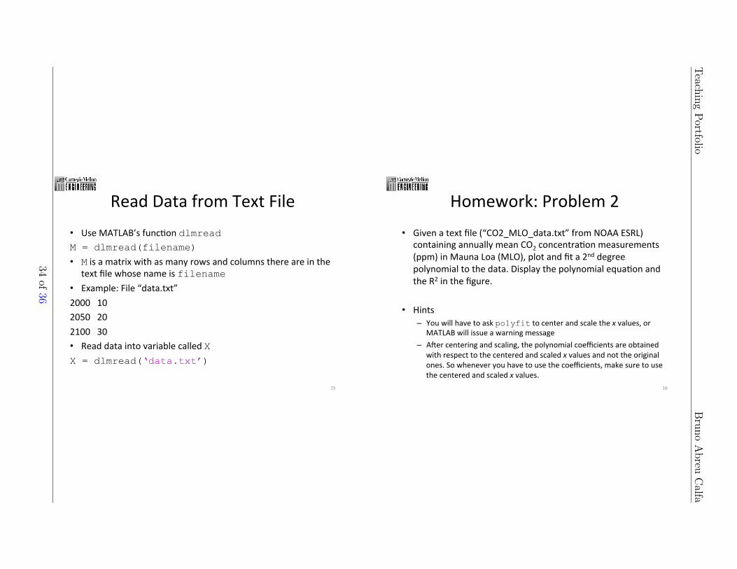
Read Data from Text File •  Use MATLAB’s func/on dlmread M = dlmread(filename)

•  M is a matrix with as many rows and columns there are in the text file whose name is filename

•  Example: File “data.txt” 2000 10 2050 20 2100 30 •  Read data into variable called X X = dlmread(‘data.txt’)

15

Homework: Problem 2 •  Given a text file (“CO2_MLO_data.txt” from NOAA ESRL)

containing annually mean CO2 concentra/on measurements (ppm) in Mauna Loa (MLO), plot and fit a 2nd degree polynomial to the data. Display the polynomial equa/on and the R2 in the figure.

•  Hints –  You will have to ask polyfit to center and scale the x values, or

MATLAB will issue a warning message –  A`er centering and scaling, the polynomial coefficients are obtained

with respect to the centered and scaled x values and not the original ones. So whenever you have to use the coefficients, make sure to use the centered and scaled x values.

16

TeachingPortfolio

Bruno

Abreu

Calfa

34of36

Air Quality at CMU

•  Center for Atmospheric Par/cle Studies (CAPS) –  hZp://caps.web.cmu.edu/members/index.html –  ChemE faculty

•  Prof. Neil Donahue (Chem) •  Prof. Spyros Pandis (EPP) •  Prof. Peter Adams (CivE, EPP)

–  Other faculty members •  Prof. Allen Robinson (MechE, EPP) •  Prof. Ryan Sullivan (Chem, MechE) •  Prof. Albert Presto (MechE)

•  Prof. Kris Dahl and I are very grateful for the ideas, materials and guidance from Prof. Neil Donahue in implemen/ng the Climate Change Module in 06-‐100 (Introduc/on to Chemical Engineering).

17

TeachingPortfolio

Bruno

Abreu

Calfa

35of36


Appendix D Teaching Assistant Award Text: AcademicYear 2011-2012

The following text was prepared and read by the Chemical Engineering Head during the2012 Department Commencement Ceremony:

“The TA award for 2012 goes to Bruno Calfa.

As the Matlab TA for John Kitchin in Fall 2011, Bruno did a spectacular job.Training in mathematical software has been an orphan topic in the department.It is vital but we have not yet found a way to incorporate it formally into thecurriculum. Prof. Kitchin and Bruno initiated a set of Matlab tutorials at thebeginning of the fall semester to address this problem. Bruno was in chargeof developing and delivering the tutorial on Matlab usage. He has since heldtutorials on other computational tools in chemical engineering including VisualBasic extensions of Excel. In addition, he helped Prof. Kitchin incorporate unitsinto Matlab. In meetings with Profs. and myself the undergraduates praisedBruno for his help.”

36 of 36

teaching portfolio - bacalfa.combacalfa.com/calfaba-teachingportfolio.pdfteachingportfolio...

Documents