Teacher peer observation and student test scores: Evidence from a field experiment in English secondary schools†

Simon Burgess, University of Bristol

Shenila Rawal, Oxford Partnership for Education Research and Analysis Eric S. Taylor, Harvard University

November 2019

This paper reports on a field experiment in 82 high schools trialing a low-cost intervention in schools’ operations: teachers from within the same school observed and scored each other’s teaching. Students in randomly-assigned treatment schools scored 0.076σ higher on math and English exams (0.097σ lower-bound on TOT). Within each treatment school, teachers were further randomly assigned to roles: observer and observee. Students in observee’s classes improved, as expected, but also so did students in observer’s classes, perhaps even slightly more so. Random variation in the number of observations through the trial produced little difference in student outcomes. JEL No. I2, M5

† Burgess: simon.burgess@bristol.ac.uk. Rawal: shenilarawal@aol.com. Taylor: eric_taylor@harvard.edu. We first thank the Education Endowment Foundation for generous financial support, the NFER for their input, as well as the Department for Education for access to the National Pupil Database. We are indebted to Julia Carey and her team for outstanding project management, and to the schools and teachers for their participation. Thanks also to Anna Vignoles, Ellen Greaves, Hans Sievertsen and seminar participants at the IZA Economics of Education Workshop, the University of Sydney, AEFP, and APPAM who provided helpful comments and questions.

1

Performance evaluation is ubiquitous in modern economies. Employers

observe and try to measure the job performance of their employees with the goal of

improving that performance. In typical practice, such performance measures are

combined with incentives; the measures determine bonuses, dismissals,

promotions, etc. Yet, evaluation might improve performance even without

attaching (explicit) incentives. The process of being measured itself could reveal

new information about an individual’s current skills or effort, or emphasize the

employer’s expectations, and thus motivate or direct an individual’s efforts to

improve. Moreover, typically the sole focus of the process is the performance of

the employee being observed; indeed the role of the observer is rarely considered,

either taken as simply another task for management, or outsourced to external

experts. Yet, in some professions and for some tasks, the observer may also gain

from the process, picking up some new ideas and practices.

In this paper’s experiment we estimate the effects of evaluation, if any,

where the potential mechanisms for those effects cannot rely on explicit incentives,

but where effects can arise through learning more about own and coworker current

performance. We take a profession with relatively well-measured inputs and

outputs, with some resistance to incentive pay, and in which observing each other

work is, while increasing, still far from commonplace. We focus on low-stakes peer

evaluation among teachers. We set up and report an experiment in which teachers

assessed and scored each other’s job performance, using structured observations of

teaching in the classroom, and discussed the results together. These peer

evaluations were “low stakes” in the sense that there were no formal incentives or

consequences attached to the scores, though there may have been informal

incentives like social pressure or career concerns. The stated goal of the program

was continuous improvement.

2

A distinctive new contribution of our experimental design is that we can

separately estimate effects on the teachers being evaluated (observees) and teachers

serving as peer evaluators (observers). Within each of the treatment schools,

individual teachers were randomly assigned to be an observee or observer or both.

Observers’ performance may suffer, for example, because they reallocate effort to

conducting evaluations; such potential losses are an important opportunity cost of

peer evaluation to weigh against benefits for observees. Observers’ performance

may also benefit from the opportunity to learn from colleagues and to reflect on

their own teaching practice. We believe that our evidence is the first to isolate the

impacts on observees and observers in this way.

A second new contribution is to examine the intensive margin of the number

of peer observations. In a random half of treatment schools, math department

teachers were expected to be observed twice as many times as their English

department colleagues; in the other half, the English department was assigned to

the double dose.

The effect of evaluation on performance is of growing interest to school

administrators and policymakers tasked with managing the teacher workforce.

Econometric research beginning in the 1970s, and accelerated in the past decade,

demonstrates educationally and economically significant differences in teachers’

contributions to their students’ learning; those differences make teachers the most

influential public input in student outcomes. However, we still understand

comparatively little about how to select better teachers, or how to train teachers

before or on the job. (For a recent review of the literature see Jackson, Rockoff, and

Staiger 2014). The importance of teachers, but lack of management tools, has

prompted new attention to teacher performance evaluation in recent years. One

common proposal is probationary screening: measure on-the-job performance early

and dismiss observed low performers (Gordon, Kane, and Staiger 2006). While the

first steps are intuitive, the equilibrium effect of this proposal likely depends more

3

on how labor supply responds than on the measurement process (Staiger and

Rockoff 2010, Rothstein 2015). A second common proposal is that the process of

evaluation itself should, if done well, improve performance (Milanowski and

Henemen 2001, Taylor and Tyler 2012). This proposal is made largely without

empirical evidence, though we discuss notable exceptions below, and the present

experiment is designed in part to help close that evidence gap.1

Our peer evaluation experiment took place over two school years in 82

secondary schools in England. In schools randomly assigned to treatment, year 10

and 11 math and English teachers were asked to participate in a new program of

peer classroom observations.2 Observer teachers visited the classrooms of observee

teachers and scored the observees using a rubric based on Charlotte Danielson’s

Framework for Teaching (2007). Within each treatment school, teachers were

randomly assigned to roles: observer, observee, or both (1/3 to each). The stated

goal was that an observee should be observed six (twelve) times per year in the low

(high) dose condition; dose was randomly assigned at the department level. Control

schools continued business as usual, which, notably, did not generally involve

teacher classroom observations by peers. The main analysis sample includes just

over 28,000 students, each with GCSE (end of year 11) test scores in math and

English, and approximately 1,300 teachers.

The paper details three main results. First, the program of low-stakes teacher

peer evaluation meaningfully improves student achievement in math and English.

Students in treatment schools scored 0.076 student standard deviations (σ) higher,

on average, than their counterparts in control schools. Nearly four of five of

1 Evaluative measures are also an important input to the long-standing proposals for teacher pay for performance. For a review of the theory and empirical literature see Neal (2011) and Jackson, Rockoff, and Staiger (2014), along with a notable more recent example Dee and Wyckoff (2015). 2 Year 10 and 11 in English schools are the final years of compulsory schooling. Students are typically 14-16 years old in these grades.

4

treatment schools completed at least some peer observations during the experiment,

suggesting a treatment-on-the-treated effect of 0.097σ at a minimum.

Second, the program benefits are not (strongly) related to the number of

peer observations, at least over the range induced by the experiment. The simple

experimental difference between outcomes in high- and low-dose conditions was -

0.002σ. A small outcome difference even though the actual number of observations

conducted did differ: high-dose departments completed nearly twice as many

observations than low-dose departments (2.9 and 1.6 per observee respectively).

Additionally, using program and dose random assignment as instruments in 2SLS,

we also fit linear and quadratic functions of the actual number of observations

conducted; the results suggest diminishing returns.

Third, student achievement improved in the classes of observee teachers as

might perhaps be expected. Our new result is that achievement also increased for

pupils of the observer teachers. We cannot reject the null hypothesis that treatment

effects are equal across the randomly-assigned teacher roles; the point estimates

are, however, larger for observers than for observees. This pattern of results rules

out the concern that benefits for observees’ students come at the expense of losses

for observers’ students. It may well be that observers’ students received less

attention from their teacher because she reallocated effort to peer evaluation, but

those costs were more than offset by benefits accrued from being an observer.

Our evidence suggests some promising leads for those designing school or

system approaches to teacher observation, with valuable improvements for a

relatively cheap and straightforward intervention. We return to discuss these

implications in the Conclusion.

These results contribute most directly to the still-small literature on how

evaluation affects teacher performance. Three papers are especially closely

5

related.3 First, studying teachers in Cincinnati, Ohio, Taylor and Tyler (2012) also

estimate the effect of a program of teacher peer evaluation based on multiple

classroom observations using a Danielson rubric. The study uses quasi-

experimental variation in the timing (the specific school year) of when a teacher

was evaluated. During the year a teacher was being evaluated her students scored

0.05σ higher in math, compared to students she taught before being evaluated, and

higher, 0.11σ, in the years after she was evaluated. Second, the Cincinnati setting

and positive effects of peer evaluation are also mirrored in recent analysis of

teachers in France (Briole and Maurin 2019).

While much is similar, including the estimated effects, between the

Cincinnati study and the present experiment, there are notable differences which

contribute to understanding potential mechanisms. In Cincinnati peer evaluator is a

full-time job given to experienced high-performing teachers; by using randomly

selected evaluators the present experiment suggests such a high-cost evaluator may

not be necessary for the benefits. Moreover, we report estimates of the effects on

the observers themselves. In Cincinnati peer evaluation scores are used for

dismissal decisions, even if rare empirically; the present experiment suggests

explicit incentives may not be necessary for teachers to put effort into the evaluation

process.

In contemporaneous work, Murphy, Weinhardt, and Wyness (2018, MWW)

study teacher peer classroom observation and feedback among year 4 and 5 teachers

in England, also using a school-level experiment. They find no effects on the

3 In a fourth related paper, Steinberg and Sartain (2015) report on a pilot-year experiment in Chicago elementary schools where the treatment was a school-wide program of teacher evaluation based on multiple classroom observations using a Danielson rubric, however, evaluations were conducted by school administrators not peers. Students scored 0.05σ higher in math and 0.10σ higher in English.

An additional experiment in several U.S. school districts, reported by Garet et al. (2017), involved a package of treatments including teacher classroom observation by school administrators, but also evaluation measures for principals and test-score based evaluation measures for teachers. The package of treatments improved student math scores by 0.05σ.

6

achievement of participating teachers’ students. The MWW treatment and our

treatment share some key features—multiple peer classroom observations, low-

stakes—but are also different in potentially important ways. The MWW treatment

is modeled on the originally-Japanese idea of “lesson study,” which is intended to

“provide a space for non-judgmental discussion” (p. 6), while our treatment is

modeled on explicit evaluation programs like the one in Cincinnati.4 Also, the

MWW treatment uses no common rubric, such as Danielson’s Framework for

Teaching, for observations and feedback. While these features are potential

explanations for effect differences, we do not have any direct tests. Before any such

direct tests, we see these studies—the present study, MWW, Taylor and Tyler, and

others—as complementary evidence in understanding the effects of evaluation on

teacher performance.

Our results on teacher roles also contribute to another implicit literature,

relevant to a practical management question, on “mentor-mentee” or “adviser-

advisee” relationships for teachers. Randomly assigning roles, as we do, is a strong

contrast to most empirical work studying such relationships. Nearly all existing

evidence comes from settings where the “advisor” or “evaluator” is (i) a formal job,

with training, filled by an experienced high-performing teacher; or (ii) a school

administrator.5 Papay, Taylor, Tyler, and Laski (in-press) study teacher pairs which

are peer coworkers, as in our present experiment, but where pairings were

intentionally based on strong-to-weak skill matching. In Murphy, Weinhardt, and

Wyness (2018) roles were assigned by the headteacher (principal). Our results

4 While neither the MWW nor our treatment included explicit or formal incentives—thus the characterization of “low stakes”—the scope for informal incentives may have differed. Because teachers were actually scored in our treatment, but not in MWW, participants may have believed those scores would end up informing future personnel decisions. 5 In the case of teacher evaluation specifically, examples of type (i) include Taylor and Tyler (2012), Dee and Wyckoff (2015), Briole and Maurin (2019), and of type (ii) Steinberg and Sartain (2015), Dee and Wyckoff (2015). For a recent review of the broader “advisor-advisee” or “coaching” literature see Kraft, Blazar, and Hogan (2018).

7

based on randomly assigned roles show benefits for both from being observed and

from doing the observing. This suggests a plausible alternative to formal, and likely

more costly, programs which use administrators or high-skilled former teachers.

In the next section we detail the treatment, setting, and data. In sections 2

and 3 we describe estimation methods and results, respectively. Results are divided

into three topics: average total effects at the school level, the relationship between

effects and the number of classroom observations, and differential effects for

observers and observees. The final section concludes.

1. Treatment, setting, and data

This paper reports on a new field experiment in which coworker teachers

observed each other teaching in the classroom, scored performance using a detailed

rubric, and discussed the results. The intervention was conducted in secondary

schools in England, focusing on years 10 and 11 math and English teachers, over

two school years, 2014-15 and 2015-16. This section describes the treatment in

detail, the study design, data, and other features of the setting.

1.1 Random assignment design, and covariate balance tests

The experiment involved randomizing aspects of the intervention at three

levels: school, department, and teacher. We first randomly assigned 82 schools, half

to the treatment—the new peer observation program—and half to a business-as-

usual control condition.6 We describe the recruitment and characteristics of the 82

schools below, as well as what “business-as-usual” means for these schools.

6 Our funder, the Education Endowment Foundation (EEF), requires that all experiments have an independent evaluator. Thus, the independent evaluator, National Foundation for Educational Research (NFER), also reported on the experiment (Worth et al. 2017). This paper and the NFER report were undertaken separately with different authors and analysis plans, and the two were planned as such from before the experiment began. Additionally, under EEF’s rules, the random assignment procedures were carried out by NFER. The procedures were jointly by the authors of this paper and NFER.

8

Schools were assigned within eight randomization blocks defined by the interaction

of three indicator variables, each indicator = 1 if the school was above the sample

median for (i) percent of students who are white, (ii) percent of students eligible for

free school meals, and (iii) prior student achievement growth at the school (school

value-added scores).

Second, we randomly assigned departments to either a “high dose” or “low

dose” condition. In half of treatment schools, the math department was assigned

“high dose” and the English department “low dose”; and in half of schools the

reverse. In the low dose condition observee teachers were expected to be observed

6 times per year. The high dose condition doubled the ask to 12. Department dose

randomization was within the same eight blocks.

Finally, within each treatment school, we randomly assigned teachers to

different roles in the program. One-third were assigned to be “observers” who

visited other teachers’ classrooms and scored the peer they watched. Observers

were not paired with observees, and could observe either math or English lessons.

One-third were assigned to be “observees” whose teaching would be observed and

scored by the observers. And the final one-third were assigned to take both observer

and observee roles. However, in eight treatment schools teacher rosters were not

available to the research team, and thus teachers in those eight schools are excluded

from the teacher role estimates.7 These eight schools are excluded from the main

comparisons by teacher role, but are included in all other estimates.

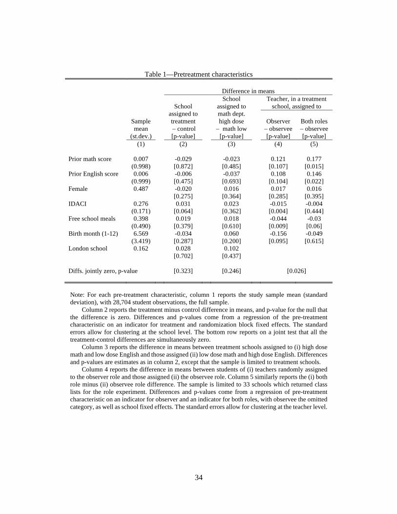
Table 1 shows the conventional pre-treatment covariate balance tests

relevant to judging the success of the random assignment. As shown in column 2,

treatment and control schools are well balanced on observables. None of the

differences are statistically significant at any conventional levels, except the

Income Deprivation Affecting Children Index (IDACI) score (𝑝𝑝 = 0.065). A given

7 While much of the data for this study was drawn from administrative data sources, as described below, we have to rely on treatment schools to provide lists of teachers and class rosters.

9

neighborhood’s IDACI score is the proportion of children under 16 living in a low-

income household; a student’s IDACI value is the score for the neighborhood where

they live.

Departments assigned to high- and low-dose are also well balanced on

observables, as shown in column 3. The difference in means reported in column 3

is between (i) treatment schools assigned to high-dose for the math department and

low-dose for English, and (ii) treatment schools assigned to the reverse case.

Last, we examine balance for the teacher role assignment experiment.

Unfortunately, we do not have data on teachers themselves, so columns 4-5

compare characteristics of students in the classrooms of observer versus observee

teachers (and both role versus observee teachers). Here, for the role assignment, we

do see differences which we would not expect after successful random assignment.

Students of observer or both-role teachers may well have higher potential GCSE

scores, compared to observee students, at least by conventional predictors.

Observer students have lower exposure to poverty in their homes and

neighborhoods, and perhaps higher prior math and English scores. Both-role

students have higher prior scores, and somewhat less exposure to poverty. Below,

after presenting the basic results on teacher role, we discuss interpretation of those

results given the imbalance in Table 1 and provide some relevant robustness tests.

1.2 Description of the treatment

The treatment, in short, is peer classroom observations among coworkers

teaching in the same school. As described above, teachers were randomly assigned

to either observe or to be observed. Each classroom observation was guided by and

scored using a detailed rubric based on Charlotte Danielson’s Framework for

Teaching (2007, “FFT”), and lasted approximately 15-20 minutes. The stated goal

was 6 or 12 observations per observee teacher per year, where 6 or 12 was randomly

10

assigned as described above. While not required, teachers were encouraged to meet

after observations to discuss feedback and share strategies for improvement.

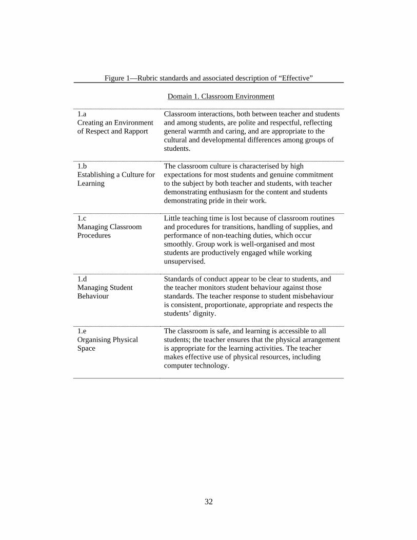
The FFT rubric is widely used by schools and in research (for example,

Kane et al. 2011, Kane et al. 2013, Bacher-Hicks et al. 2017). The rubric is divided

into four “domains”—classroom environment, instruction, planning, and

assessment—with several “standards” within each domain. In the current

experiment, classroom observations used only the “classroom environment” and

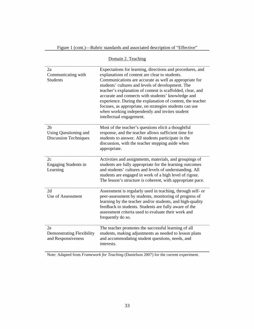
“teaching” domains, which are measured while watching teachers teach. In Figure

1 the left-hand column lists the ten standards on which teachers were evaluated. For

each standard, the rubric includes descriptions of what observed behaviors should

be scored as “Highly Effective” teaching, “Effective,” “Basic,” and “Ineffective.”

In Figure 1 we reproduce the descriptions for “Effective” as an example. The full

rubric is provided in the Appendix. The current experiment’s rubric language

differs slightly from the standard FFT rubric descriptions; the text was edited

slightly to be more appropriate for the English school setting.

The FFT, and other similar observation rubrics and protocols, were not

explicitly designed as a tool to improve student achievement scores, as we measure

in this experiment. Nevertheless, existing evidence is consistent with expecting

positive effects of this “treatment.” First, several studies now find a similar, if

moderate, positive correlation between observation scores and student test scores,

including some settings where students are randomly assigned to teachers (Kane et

al. 2011, Kane et al. 2013, Garrett and Steinberg 2015, Araujo et al. 2016, Bacher-

Hicks et al. 2017). Second, as cited in the introduction, a growing number of

(quasi)-experimental studies document positive effects on student achievement of

programs where teachers are observed and scored using FFT or similar rubrics

(Taylor and Tyler 2012, Steinberg and Sartain 2015, Garet et al. 2017, Briole and

Maurin 2019).

11

Conventionally the FFT rubric is scored on a 1-4 integer scale, with 1-4

corresponding to “Ineffective” through “Highly Effective”. We instead asked

observers to use a 1-12 integer scale where 12 was “Highly Effective+”, 11 “Highly

Effective”, 10 “Highly Effective−", 9 “Effective+”, and so on. The 1-12 scale was

motivated in part by the typical skewness toward scores of 3-4 on evaluation ratings

using a 1-4 scale generally, and with teacher observation rubrics specifically (Kane

et al. 2011, Kraft and Gilmour 2016). This tendency was confirmed in our pilot

stage work with schools.8

In addition to the FFT-based assessments of teaching quality, we also asked

observers to record other relatively-objective data on teaching practices. For

example, how often—never, some of the time, all of the time—the teacher lectured

the whole class, had students work in small groups, or taught students one-on-one.

These measures were also drawn from previous research, and the complete

instrument is provided in the Appendix.

Teachers were provided training on the FFT rubric and other aspects of the

program, primarily in-person training but supplemented with phone and email

conversations. Treatment schools were also given a few tablet computers to

facilitate observations. Observers could access the complete FFT rubric, record

scores, and make notes during their observations.9 The centrally-stored database of

observations allowed the research team to monitor progress of individual schools,

and contact those who were clearly lagging. However, the specific schedule and

pace of observations was left to each school to determine.

8 Pooling the 10 standards, the average rubric item score was 9.05 with a standard deviation of 2.10. If we convert the 1-12 scale to the more common 1-4 scale (i.e., 12 = 4.33, 11 = 4, 10 = 3.66, 9 = 3, and so on) the average item score is 3.35 (st.dev. 0.70). This mean is quite similar to other contexts, for example, Kane et al. (2011) where the mean is 3.23. However, in our setting the standard deviation is a wider 0.70 versus, for example, 0.49 in Kane et al. (2011). The wider variation may be due in part to the 1-12 scale. 9 The tablets were Apple iPads, and the software was created by RANDA Solutions.

12

1.3 Evaluation and classroom observation in English secondary schools

Classroom observations of teaching are certainly not new to the schools we

study, and observations were likely occurring in control schools during the study.

However, the treatment observations had three (potentially) first-order features

distinct from business-as-usual in English secondary schools: observation by peer

teachers, observations based on an FFT-style rubric, and simply more observations

regardless of who or what rubric.

In our conversations with study schools, most reported that some form of

class observations were part of their normal business. In contrast to the treatment

peer observations, these school-initiated observations were conducted by school

leaders, unstructured, and much rarer. The average teacher would be observed

perhaps once per year and often less than annually. Moreover, the frequency of

observations was curtailed partly by union opposition, sometimes codified into

rules limiting observations. Consistent with this description of limited status-quo

observation, treatment teachers reported appreciating that the program included

more frequent observations and observations from peers instead of school leaders.

Beyond school-initiated efforts, classroom observations occur for two other

reasons. First, observations are part of the formal induction and assessment process

for novice teachers, known as “NQT teachers” or the “NQT year” (NQT = newly

qualified teacher). An NQT teacher might be observed as many as six times, but

the teachers are typically only NQT for one year.

Second, observations are part of England’s formal performance evaluation

process for schools. The school inspection process, conducted by the Office of

Standards in Education, Children’s Services and Skills (Ofsted), does include

classroom observations among many other forms of evaluation. However, Ofsted’s

classroom observations are not salient to individual teachers. During a school

inspection Ofsted observers visit several teachers’ classes, but far from all teachers;

the goal of Ofsted’s observations is to make overall assessments of teaching in the

13

school, not of each individual teacher. Moreover, a typical school might only be

visited by Ofsted every 3-4 years. In short, the chances of a given teacher in a given

year being observed by Ofsted are low, and there would be little individual

consequence of the results.10

1.4 Sample and data

Our study sample is composed of 82 schools, over 28,000 students with

GCSE math and English test scores, and approximately 1,300 teachers. We initially

contacted almost all high-poverty public (state) secondary schools and invited them

to participate in the study.11 School performance levels (test scores) were not used

as a criterion for inviting schools. Of the invited schools, 93 responded and

volunteered to participate (8.5 percent). We randomized 82 schools to treatment

and control; ten schools dropped out before randomization and one was excluded

by the research team12. The schools initially invited were intentionally selected to

have high poverty rates. These characteristics are reflected in the study sample, as

shown in Table 1 column 1. Nearly 40 percent of students are (or ever have been)

eligible for free school meals, substantially higher than the national average.

Much of the data for our analysis come from the UK government’s National

Pupil Database (NPD). These administrative data include student level records with

math and English GCSE scores, prior test scores (KS2), demographic and other

characteristics of students, and their school. The NPD data are sufficient for our

ITT estimates of average treatment effect.

10 Ofsted and the Department for Education (DfE) also set expectations and guidelines for each school’s own self-evaluation practices. Classroom observations broadly-speaking should be part of each school’s plans, but Ofsted and DfE do not require a specific minimum number, type of observer, or criteria for what should be evaluated in the observation. Moreover, until recently there was a rule limiting observations to no more than three per year. 11 We excluded, ex-ante, boarding schools, single-gender schools, as well as schools in select geographic areas where the funder was conducting different interventions. The final list invited was 1,097 schools. 12 The school was in Wales rather than England and so was not in the NPD.

14

We add to the NPD data in two ways. First, the data recorded during peer

observations allow us to measure participation, for example, the number of

observations completed for a given school, department, or teacher. The data also

include observation scores, which, at present, we do not use in this paper. Second,

we asked treatment schools to provide a list of their math and English teachers, and

the specific year 10 and 11 students assigned to those teachers. We link these rosters

to NPD data using unique student IDs, and to the observation data using teacher

IDs created for this study. Additionally, the teachers listed in these rosters were the

teachers included in the role randomization. Note that we lack these teacher-student

linking rosters for 8 of the 41 treatment schools.13

Our estimates are not threatened by attrition, at least not in the first-order

sense of attrition. The NPD data include the universe of students and schools. Thus,

even if a school chose to withdraw from the study, we observe outcomes and can

still include the school in our analysis. If, however, treatment induced students to

move to different schools at a rate higher (lower) than control schools, those

movements would be relevant to the interpretation of our results. Treatment effects

on student school switching seems unlikely. Treatment effects on teachers

switching schools may be more plausible. Our analysis of differences between

teacher roles uses teacher’s class rosters provided at the beginning of each school

year, in the spirit of intent-to-treat. We cannot observe teacher movements between

schools in the data as we do not know teacher names, but any such moves induced

by treatment would be relevant to interpreting our results.

13 Some schools never provided complete rosters. In other cases, the school provided the rosters, but subsequently withdrew from the study and asked that their previously-provided rosters not be used in the research.

15

2. Analysis methods

Our analysis of the experiment data follows conventional experimental

methods. To begin we estimate the difference between average student GCSE

scores in treatment and control schools by fitting the following regression

specification:

𝑌𝑌𝑖𝑖𝑖𝑖𝑖𝑖 = 𝛿𝛿𝑇𝑇𝑠𝑠 + 𝜋𝜋𝑏𝑏 + 𝑋𝑋𝑖𝑖𝛽𝛽 + 𝜀𝜀𝑖𝑖𝑖𝑖𝑖𝑖

(1)

where 𝑌𝑌𝑖𝑖𝑖𝑖𝑖𝑖 is the GCSE score for student 𝑖𝑖 in subject 𝑚𝑚 (math or English) taken in

year 𝑡𝑡 (2015 or 2016). Student scores, 𝑌𝑌𝑖𝑖𝑖𝑖𝑖𝑖, are standardized (mean 0, s.d. 1) by

subject and year within our analysis sample. The indicator 𝑇𝑇𝑠𝑠 = 1 for all schools 𝑠𝑠

randomly assigned to the treatment, and 𝜋𝜋𝑏𝑏 represents fixed effects for the eight

blocks 𝑏𝑏 within which random assignment occurred.14 The vector 𝑋𝑋𝑖𝑖 includes the

student characteristics measured pre-treatment listed in Table 1, most notably prior

achievement scores in math and English, along with a cohort dummy (the year the

exams were taken) and a subject dummy (math or English). We report

heteroskedasticity-cluster robust standard errors where the clusters are schools 𝑠𝑠,

the unit at which treatment is assigned.15

Fitting specification 1 returns intent-to-treat effects. We also report

treatment-on-the treated estimates where 𝑇𝑇𝑠𝑠 is replaced with an indicator if the

school actually implemented the peer observation program, and we instrument for

that endogenous treatment indicator with the randomly assigned 𝑇𝑇𝑠𝑠. Because the

latent characteristic “implemented” is not binary, we show a few different

alternatives for the endogenous treatment indicator.

14 Students are nested in schools, 𝑠𝑠 = 𝑠𝑠(𝑖𝑖), and schools are nested in randomization blocks, 𝑏𝑏 =𝑏𝑏(𝑠𝑠). To streamline the presentation we use the simple 𝑠𝑠 and 𝑏𝑏 subscripts. 15 Our main estimates pool subjects. Students’ math and English score errors are also likely correlated. Since students are nested within schools, clustering by school is identical to clustering by school and student.

16

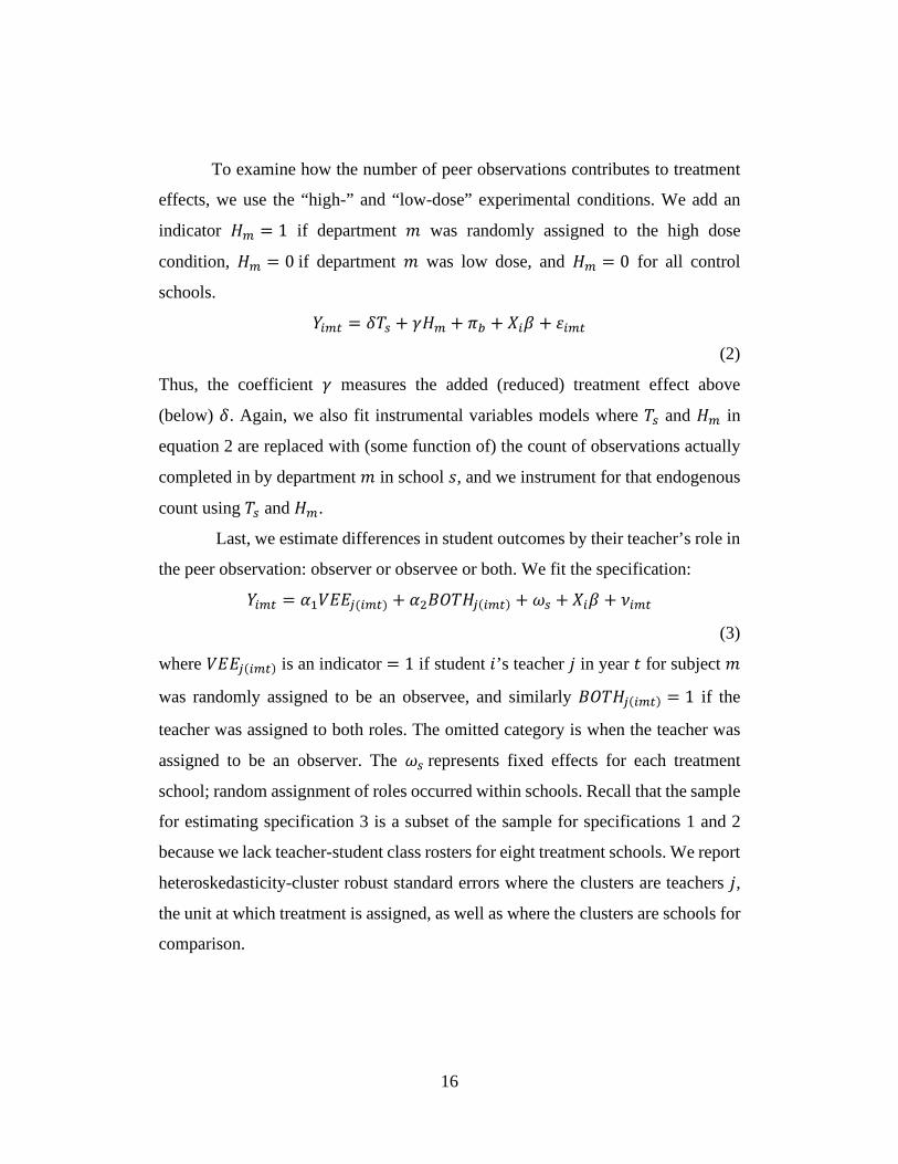
To examine how the number of peer observations contributes to treatment

effects, we use the “high-” and “low-dose” experimental conditions. We add an

indicator 𝐻𝐻𝑖𝑖 = 1 if department 𝑚𝑚 was randomly assigned to the high dose

condition, 𝐻𝐻𝑖𝑖 = 0 if department 𝑚𝑚 was low dose, and 𝐻𝐻𝑖𝑖 = 0 for all control

schools.

𝑌𝑌𝑖𝑖𝑖𝑖𝑖𝑖 = 𝛿𝛿𝑇𝑇𝑠𝑠 + 𝛾𝛾𝐻𝐻𝑖𝑖 + 𝜋𝜋𝑏𝑏 + 𝑋𝑋𝑖𝑖𝛽𝛽 + 𝜀𝜀𝑖𝑖𝑖𝑖𝑖𝑖

(2)

Thus, the coefficient 𝛾𝛾 measures the added (reduced) treatment effect above

(below) 𝛿𝛿. Again, we also fit instrumental variables models where 𝑇𝑇𝑠𝑠 and 𝐻𝐻𝑖𝑖 in

equation 2 are replaced with (some function of) the count of observations actually

completed in by department 𝑚𝑚 in school 𝑠𝑠, and we instrument for that endogenous

count using 𝑇𝑇𝑠𝑠 and 𝐻𝐻𝑖𝑖.

Last, we estimate differences in student outcomes by their teacher’s role in

the peer observation: observer or observee or both. We fit the specification:

𝑌𝑌𝑖𝑖𝑖𝑖𝑖𝑖 = 𝛼𝛼1𝑉𝑉𝑉𝑉𝑉𝑉𝑗𝑗(𝑖𝑖𝑖𝑖𝑖𝑖) + 𝛼𝛼2𝐵𝐵𝐵𝐵𝑇𝑇𝐻𝐻𝑗𝑗(𝑖𝑖𝑖𝑖𝑖𝑖) + 𝜔𝜔𝑠𝑠 + 𝑋𝑋𝑖𝑖𝛽𝛽 + 𝜈𝜈𝑖𝑖𝑖𝑖𝑖𝑖

(3)

where 𝑉𝑉𝑉𝑉𝑉𝑉𝑗𝑗(𝑖𝑖𝑖𝑖𝑖𝑖) is an indicator = 1 if student 𝑖𝑖’s teacher 𝑗𝑗 in year 𝑡𝑡 for subject 𝑚𝑚

was randomly assigned to be an observee, and similarly 𝐵𝐵𝐵𝐵𝑇𝑇𝐻𝐻𝑗𝑗(𝑖𝑖𝑖𝑖𝑖𝑖) = 1 if the

teacher was assigned to both roles. The omitted category is when the teacher was

assigned to be an observer. The 𝜔𝜔𝑠𝑠 represents fixed effects for each treatment

school; random assignment of roles occurred within schools. Recall that the sample

for estimating specification 3 is a subset of the sample for specifications 1 and 2

because we lack teacher-student class rosters for eight treatment schools. We report

heteroskedasticity-cluster robust standard errors where the clusters are teachers 𝑗𝑗,

the unit at which treatment is assigned, as well as where the clusters are schools for

comparison.

17

A causal interpretation of our key estimates—𝛿𝛿, 𝛾𝛾�, 𝛼𝛼�1, and 𝛼𝛼�2—requires

the conventional experimental identification assumption: In the absence of the

experiment, students in treatment and control schools (high- and low-dose

departments, observee and observer teacher classes) would have had equal GCSE

scores at expectation. Balance in pre-treatment covariates (Table 1) across

treatment and control schools and high- and low-dose departments is consistent

with this assumption. By contrast, the imbalance across observer and observee

classrooms suggests caution giving a strong causal interpretation to 𝛼𝛼�1 and 𝛼𝛼�2. We

return to the interpretation of the role differences below.

3. Results

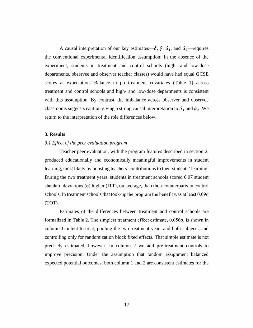
3.1 Effect of the peer evaluation program

Teacher peer evaluation, with the program features described in section 2,

produced educationally and economically meaningful improvements in student

learning, most likely by boosting teachers’ contributions to their students’ learning.

During the two treatment years, students in treatment schools scored 0.07 student

standard deviations (σ) higher (ITT), on average, than their counterparts in control

schools. In treatment schools that took-up the program the benefit was at least 0.09σ

(TOT).

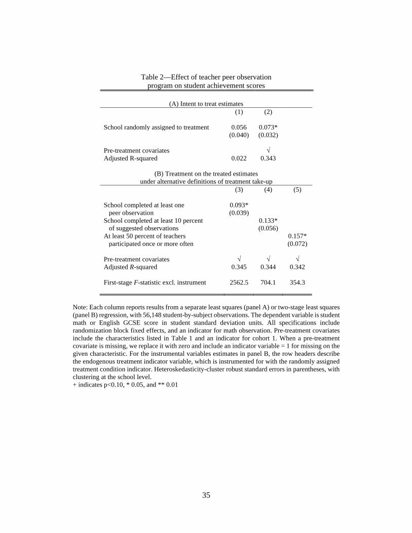
Estimates of the differences between treatment and control schools are

formalized in Table 2. The simplest treatment effect estimate, 0.056σ, is shown in

column 1: intent-to-treat, pooling the two treatment years and both subjects, and

controlling only for randomization block fixed effects. That simple estimate is not

precisely estimated, however. In column 2 we add pre-treatment controls to

improve precision. Under the assumption that random assignment balanced

expected potential outcomes, both column 1 and 2 are consistent estimates for the

18

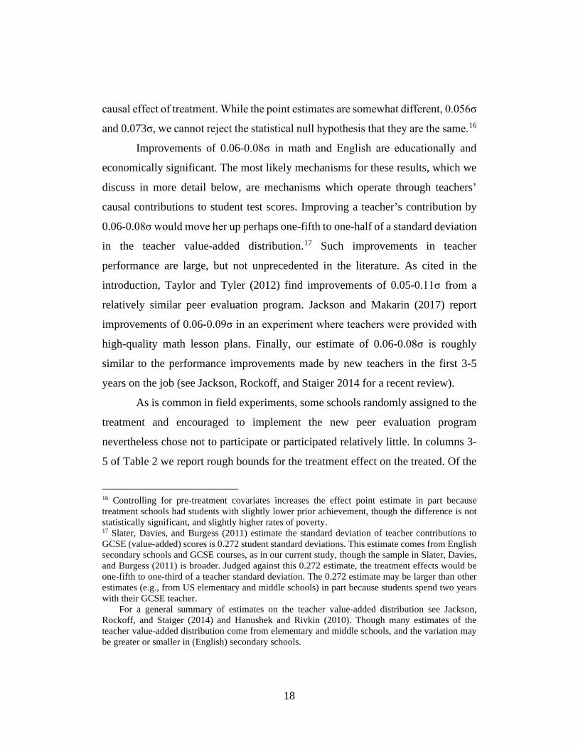
causal effect of treatment. While the point estimates are somewhat different, 0.056σ

and 0.073σ, we cannot reject the statistical null hypothesis that they are the same.16

Improvements of 0.06-0.08σ in math and English are educationally and

economically significant. The most likely mechanisms for these results, which we

discuss in more detail below, are mechanisms which operate through teachers’

causal contributions to student test scores. Improving a teacher’s contribution by

0.06-0.08σ would move her up perhaps one-fifth to one-half of a standard deviation

in the teacher value-added distribution.17 Such improvements in teacher

performance are large, but not unprecedented in the literature. As cited in the

introduction, Taylor and Tyler (2012) find improvements of 0.05-0.11σ from a

relatively similar peer evaluation program. Jackson and Makarin (2017) report

improvements of 0.06-0.09σ in an experiment where teachers were provided with

high-quality math lesson plans. Finally, our estimate of 0.06-0.08σ is roughly

similar to the performance improvements made by new teachers in the first 3-5

years on the job (see Jackson, Rockoff, and Staiger 2014 for a recent review).

As is common in field experiments, some schools randomly assigned to the

treatment and encouraged to implement the new peer evaluation program

nevertheless chose not to participate or participated relatively little. In columns 3-

5 of Table 2 we report rough bounds for the treatment effect on the treated. Of the

16 Controlling for pre-treatment covariates increases the effect point estimate in part because treatment schools had students with slightly lower prior achievement, though the difference is not statistically significant, and slightly higher rates of poverty. 17 Slater, Davies, and Burgess (2011) estimate the standard deviation of teacher contributions to GCSE (value-added) scores is 0.272 student standard deviations. This estimate comes from English secondary schools and GCSE courses, as in our current study, though the sample in Slater, Davies, and Burgess (2011) is broader. Judged against this 0.272 estimate, the treatment effects would be one-fifth to one-third of a teacher standard deviation. The 0.272 estimate may be larger than other estimates (e.g., from US elementary and middle schools) in part because students spend two years with their GCSE teacher.

For a general summary of estimates on the teacher value-added distribution see Jackson, Rockoff, and Staiger (2014) and Hanushek and Rivkin (2010). Though many estimates of the teacher value-added distribution come from elementary and middle schools, and the variation may be greater or smaller in (English) secondary schools.

19

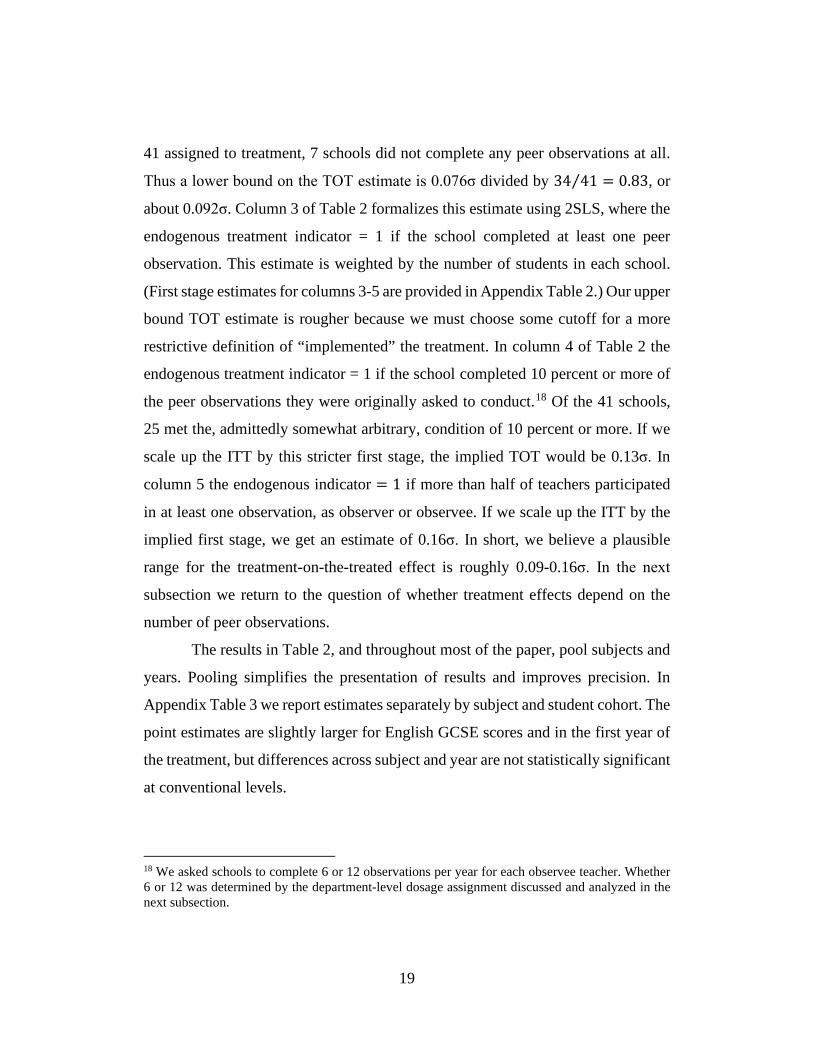
41 assigned to treatment, 7 schools did not complete any peer observations at all.

Thus a lower bound on the TOT estimate is 0.076σ divided by 34 41⁄ = 0.83, or

about 0.092σ. Column 3 of Table 2 formalizes this estimate using 2SLS, where the

endogenous treatment indicator = 1 if the school completed at least one peer

observation. This estimate is weighted by the number of students in each school.

(First stage estimates for columns 3-5 are provided in Appendix Table 2.) Our upper

bound TOT estimate is rougher because we must choose some cutoff for a more

restrictive definition of “implemented” the treatment. In column 4 of Table 2 the

endogenous treatment indicator = 1 if the school completed 10 percent or more of

the peer observations they were originally asked to conduct.18 Of the 41 schools,

25 met the, admittedly somewhat arbitrary, condition of 10 percent or more. If we

scale up the ITT by this stricter first stage, the implied TOT would be 0.13σ. In

column 5 the endogenous indicator = 1 if more than half of teachers participated

in at least one observation, as observer or observee. If we scale up the ITT by the

implied first stage, we get an estimate of 0.16σ. In short, we believe a plausible

range for the treatment-on-the-treated effect is roughly 0.09-0.16σ. In the next

subsection we return to the question of whether treatment effects depend on the

number of peer observations.

The results in Table 2, and throughout most of the paper, pool subjects and

years. Pooling simplifies the presentation of results and improves precision. In

Appendix Table 3 we report estimates separately by subject and student cohort. The

point estimates are slightly larger for English GCSE scores and in the first year of

the treatment, but differences across subject and year are not statistically significant

at conventional levels.

18 We asked schools to complete 6 or 12 observations per year for each observee teacher. Whether 6 or 12 was determined by the department-level dosage assignment discussed and analyzed in the next subsection.

20

3.2 Treatment effects and the number of peer observations

A first-order design feature of a teacher observation program, like the one

we study, is the number of classroom observations conducted. Our treatment effect

estimates, discussed in the previous subsection, are effects for the average treatment

school. The corresponding number of observations completed by the average

treatment school is 2.27 per observee teacher per year (standard deviation 2.67).

The natural follow-up question is: Would the estimated average treatment effect be

larger or smaller than 0.06-0.08σ if the number of observations conducted were

larger or smaller? Are the marginal returns linear, increasing, decreasing? In this

subsection we provide some estimates relevant to these questions, but our answers

are constrained by the variation in our experiment.

The cleanest result comes from direct experimental variation in the number

of observations. Recall that, within each treatment school, one of the two

departments (math or English) was randomly assigned to a low-dose condition of

six observations per observee per year, and thus the other of the two departments

(English or math) was randomly assigned to a high-dose condition of twelve

observations. The average number of observations actually conducted was 1.6 and

2.9 in the normal- and double-dose conditions respectively (see the first stage

results in Appendix Table 4). Actual observations were certainly short of what

teachers were initially asked to do, but the difference in actual observations caused

by the dosage random assignment was still nearly a doubling of observations.

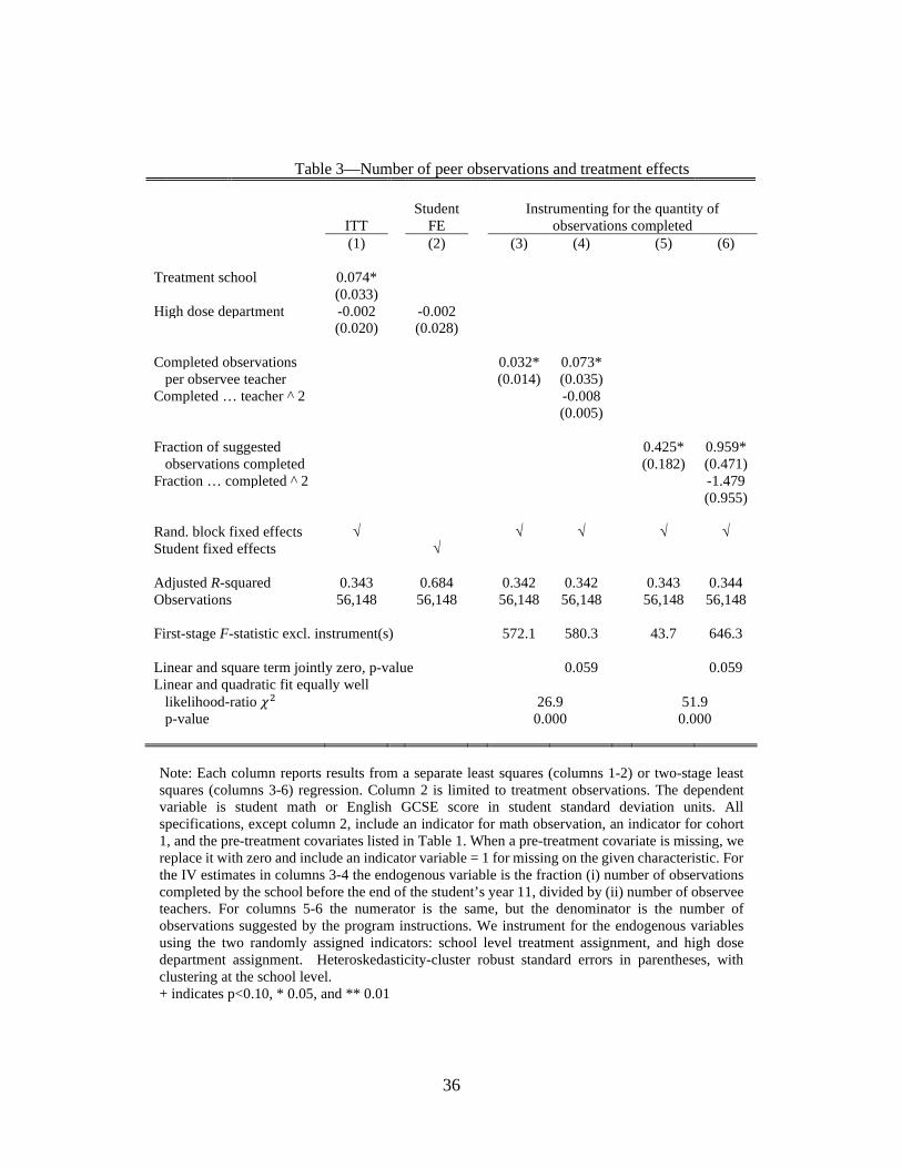
That experimental doubling of observations did not, however, increase the

treatment effect. In Table 3 column 1 we show ITT estimates from a specification

identical to Table 2 column 2 except that we have added a right-hand-side indicator

= 1 if the department was randomly assigned to the high-dose condition (the new

indicator is zero for all control cases). The estimated effect is close to zero, -0.002σ,

and far from statistically significant. This test, though blunt, suggests little

21

covariance between treatment effects and number of observations over the range of

1.6-2.9 observations.19

Table 3 also reports estimates of the relationship between student

achievement scores and the actual number of observations completed per observee

teacher. These are 2SLS estimates where we instrument for actual observations

with two random assignment indicators: school-level treatment and department-

level high-dose.20 The estimated marginal benefit of an additional observation per

observee is 0.032σ if we restrict the relationship to be linear (column 3).

Alternatively, if we allow a quadratic relationship, the marginal benefits are

somewhat larger near the sample mean, but then diminishing (column 4). We can

reject the null hypothesis that the linear fits the data as well as the quadratic. As

shown in columns 5-6, this pattern of results is the same if we use a different

measure of observations completed: the proportion of suggested observations

completed.

Taken together the results in Table 3 are somewhat ambiguous. The reduced

form estimates in column 1 suggest no relationship between treatment effects and

number of observations. The 2SLS estimates in columns 3-6, by contrast, suggest

a positive, diminishing relationship. Both the reduced form and 2SLS estimates rely

on the same fundamental identifying variation arising from random assignment.

The 2SLS estimates, however, require an additional parametric assumption about

the relationship (linear or quadratic).21 If that assumption is incorrect, then the

19 The estimates in Table 3 column 1 are identified by random assignment. As a robustness check, in column 2 we estimate a student fixed effects version of equation 2. The results are the same. 20 The first stage results are provided in Appendix Table 4. The endogenous variable is the total number of lessons observed for department d in school s for cohort 𝑡𝑡, divided by the number of observees in the same cell. This variable is zero in all control school cases. 21 The 2SLS estimates also require an exclusion restriction, which seems reasonable given that the instruments are randomly assigned.

22

2SLS estimates may be misleading. Appendix Figure 1 provides some evidence, if

imperfect and noisy, suggesting the parametric assumptions are reasonable.22

3.3 Treatment effects and teacher roles

Another first-order feature of a teacher observation program is deciding

who should be observed (observee) and by whom (observer). By randomly

assigning these teacher roles, our experiment contributes distinctively new

evidence to the literature on teacher peer evaluation, the first to estimate the impact

on observers. First, the estimates of total effect and dosage presented above are not

(less likely) driven by selecting observers and observees on some (un)observable

potential outcomes. To this point in the paper the results presented have pooled all

teachers and students regardless of role. Second, in this subsection we estimate

treatment effects separately for observer and observee teachers.

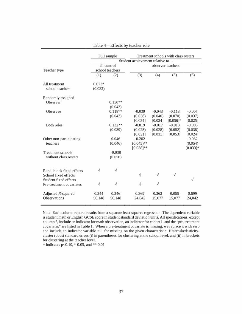
Table 4 shows test score differences by teacher role. We begin with a

regression that includes all teachers and schools in the study. For convenience,

Table 4 column 1 repeats Table 2 column 2—our main between-school treatment-

control difference. In Table 4 column 2, the omitted category remains all control

schools and teachers, but we now divide treatment school students into five

mutually exclusive and exhaustive groups. Groups (i)-(iii) are the students of

teachers who were randomly assigned to the experiment roles (i) observer, (ii)

observee, and (iii) both roles. For example, students in the classrooms of observer

teachers scored 0.15σ higher than the average control student. Group (iv) is students

assigned to all other teachers in treatment schools; teachers who did not participate

22 In Appendix Figure 1 we provide some less-parametric evidence on the relationship between outcomes and number of observations per observee. First, for each treatment school, we calculate the school’s mean GCSE test score, minus the overall control mean score. This estimate is not, strictly speaking, a school specific treatment effect estimate identified by random assignment, but we think it is informative. Second, we plot these 41 estimates against the number of observations completed per observee, and fit a lowess line. The fitted line suggests increasing returns at low levels of observations (less than 2-3), but flat returns after that point.

23

in peer observation experiment, and thus were not assigned a role. Non-

participating teachers include temporary teachers—called cover teachers in

England (long-term substitutes in the US)—as well as other teachers excluded by

their schools for other reasons. Group (v) is all students in the eight treatment

schools where we do not have any student-teacher class rosters.23

The differences in Table 4 column 2 are not strictly identified by random

assignment, however. Only the groups (i)-(iii) were randomly assigned. The

expected student score in the control group, as a whole, is not necessarily an

appropriate counterfactual for any one of the five groups shown in column 2.

The cleanest, intent-to-treat results for the role experiment are in Table 4

column 4. The differences in column 4 are by design identified by random

assignment. The sample is limited to teachers and schools which participated in the

role random assignment, and we use only variation within schools.

The students of observer teachers scored higher, on average, than the

students of teachers who were observed by 0.043σ, but the difference is not

statistically significant at any conventional level. Scores for “both role” teachers

are between observers and observees, but again not statistically different.

Additionally, we find little difference across assigned roles in extensive or intensive

margins of actual participation in peer observations, so that treatment-on-the-

treated estimates show the same pattern as in Table 4 column 4.24

These results imply that the average treatment effects, reported in Table 2,

are shared relatively evenly by both observer and observee teachers. Similar effects

do not necessarily imply similar mechanisms, however, and we return to a

23 As a robustness check, we re-estimate the overall treatment effects in Table 2 dropping these eight schools. The estimates are larger: 0.10σ for the ITT with covariates, and 0.11σ for our lower-bound TOT. These larger estimates are partly a reflection of the correlation between providing rosters and participating in other ways. 24 2SLS TOT estimates and associated first stages for the role experiment are provided in Appendix Tables 5 and 6 respectively.

24

discussion of mechanisms for observers and observees below. These results also

rule out the hypothesis that benefits for observees come at the opportunity cost of

reduced achievement in observers’ classrooms as observers shift effort or time to

observations. There may well have been such opportunity costs, but they were

offset by gains for the observers.

For one final observation about mechanisms we return to Table 4 column

3. As in column 4 we find little difference across the randomly assigned teacher

roles. By contrast, the students of other non-participating teachers scored noticeably

lower than their schoolmates in observers’ and observees’ classrooms; a difference

of -0.202σ. This pattern would be consistent with effects for participating teachers,

but no (small) spillovers to non-participating teachers. But this pattern could also

be consistent with some selection of teachers into the role experiment randomly-

assigned sample, presumably by school administrators but based on factors

unobservable to us. Regarding this second explanation, we do not have pre-

treatment teacher performance measures, but we can compare students’ pre-

treatment characteristics and we find no differences for participating and non-

participating classrooms.

3.3.1 Robustness

An interpretation of the differences between roles—the results in Table 4

column 4—as causal relies on the random assignment successfully balancing

potential outcomes, as noted above. The conventional test of balance is to compare

pre-treatment covariates across conditions, and, as shown in Table 1, there is

imbalance on prior student achievement and poverty measures. We can and do

control for these observable differences, but, as always, the concern is that

observable differences suggest scope for unobserved differences. In the end, this

imbalance should add caution to a strong causal interpretation of the differences

25

between roles. However, in this section we provide evidence to inform judgements

about the potential bias from this imbalance.

The first result is simply to re-estimate Table 4 column 4 without the pre-

treatment covariates, as shown in Table 4 column 5. These point estimates are

larger, as expected given the imbalance, but still not statistically significantly

different. Thus, no change to the substantive conclusion that treatment effects were

similar across roles.

For a second robustness test we use only within student variation:

differences, for a given student, in her math teacher’s role and her English teacher’s

role. These student fixed effects estimates, in Table 4 column 6, are consistent with

our main estimates: no differences between observers and observees. Again these

are assigned roles, thus in the spirit of ITT. Also consistent, achievement was about

0.08σ higher in the subject where a student’s teacher was assigned to a role in the

peer evaluation compared to the subject where the student’s teacher was not

involved. Student fixed effects weaken the identifying assumption. In the

conventional experiment, sorting between students would potentially threaten

identification. With student fixed effects, threats require sorting based on

differences in math and English potential outcomes for a given student.

A third robustness test builds on the fact that role assignment occurred

within each treatment school. We can thus estimate the degree of pre-treatment

covariate (im)balance for each school, and then see whether treatment effects

covary with the estimate of (im)balance. In Appendix Table 7 we show estimates

like Table 4 column 4 separately for two subsamples of treatment schools

segmented into relatively “low imbalance” and “high imbalance” in the following

way. First, for each student, we convert the available pre-treatment covariates into

a scalar index measure. Using the control sample, we regress GCSE score on those

covariates, and then calculate the fitted GCSE score for treatment cases. That fitted

score is our index. Second, for each school, we estimate the mean difference in that

26

index between observers and observees. We define relatively “low imbalance”

schools as schools where the absolute fitted-score difference of less than 0.10σ, and

“high imbalance” schools those with 0.10σ or greater. In the relatively low

imbalance schools, the pattern of effects mirrors the main estimates in Table 4

column 4: small differences which are not statistically significant. However, we

cannot say what made some schools “low imbalance” and others “high imbalance,”

and so we are cautious about generalizing the results.25

4. Conclusion

In this paper we report improvements in teachers’ job performance, as

measured by their contributions to student test scores, resulting from a program of

low-stakes peer evaluation. In randomly assigned treatment schools, teachers

visited the classrooms of other teachers in the school, and scored the teaching they

observed using a structured rubric. Students in treatment schools scored 0.07

student standard deviations (σ) higher on high-stakes GCSE exams in math and

English (ITT estimate). In treatment schools which took-up the program students

cored at least 0.09σ higher (minimum TOT estimate). Explanations for the effects

of this peer evaluation cannot be based on explicit incentive structures typical in

other formal evaluation settings as these were absent by design; rather the effects

likely operate through new information about individual performance as well as

interaction among peer coworkers.

25 The results by teacher role are also robust to how we pool observations. The experiment included teachers of year 10 and year 11 students over two school years. Our data include “Cohort 1” students who where in year 11 in the experiment’s first year, and took their GCSE exams at the end of that year. And “Cohort 2” who were in year 10 in the experiment’s first year, then year 11 the experiment’s second year, and thus took GCSEs at the end of year two. Most “Cohort 2” students had the same teacher (and thus the same role indicator variables) in both years. However, we estimated role differences separately using (i) Cohort 1, year 11 teacher, (ii) Cohort 2, year 10 teacher, and (iii) Cohort 2, year 11 teacher to construct the role indicators. The results are consistent across these approaches, as shown in Appendix Table 8a and 8b.

27

The school-level results we report contribute to a small literature on how

evaluation, in different forms, affects teacher job performance (e.g., Taylor and

Tyler 2012, Steinberg and Sartain 2015, Bergman and Hill 2015, Dee and Wyckoff

2015, Briole and Maurin 2019). Our school-level estimates are broadly consistent

with similar treatments in quite different settings. For example, Taylor and Tyler

(2012) report quasi-experimental estimates of the effect of evaluation using rubric-

based classroom observations. They find teacher performance improved by 0.05-

0.11σ in a rather different setting to ours: younger pupils (grades 4-8); evaluation

with explicit consequences for the teachers; and the evaluators were trained,

external specialists. Steinberg and Sartain (2015) find similar results when the

evaluators are school principals. In contemporaneous work, Murphy, Weinhardt,

and Wyness (2018) find that teacher performance did not significantly change in

an experimental implementation of “lesson study” in primary schools (other

operational differences from our study are noted above).

The main new contribution of the paper is based on our randomization of

teacher roles, allowing us to estimate the benefits to the different evaluation roles.

We believe this is the first experimental evidence on the job performance benefits

to the observers in a teacher evaluation program. As might be expected, the

observed teachers do benefit from peer observation, as measured by the test score

gains of their pupils. We show that the pupils of the observing teachers also benefit,

and perhaps to a greater extent than the teachers they observe. The most likely

interpretation of this is that the observers learn new ideas for their own teaching

and have an opportunity to reflect on their own practice in a non-challenging

setting. The implication of this is quite striking: schools that out-source the

evaluator role and schools in which observation/evaluation are just another task for

school leaders are missing out on more than half of the potential gain to observation.

The benefits of peer evaluation documented in this experiment suggest

practical and promising policy ideas for improving the job performance of a sizable

28

workforce. Relative to other educational interventions, this program seems both

politically and financially attractive. Politically, the program is likely less

threatening because of the absence of strong or explicit consequences attached to

the scores, and because observers are peers rather than outside experts or school

leaders. Financially because it is a cheap intervention, at least in budget terms. The

first-order costs of the program are the opportunity costs of participating teachers’

time. Potential forgone uses of teachers’ time and effort include (i) attention to their

current students (or other job responsibilities), (ii) other investments in developing

new or existing skills, or (iii) teachers’ own leisure. These opportunity costs are

potentially offset, as we find, when observers themselves improve as a result of

their role. Indeed, schools or school systems that pay for external evaluators pay

twice: the fee for the service and the lost learning experiences for the school’s own

teachers.

29

References

Araujo, M. C., Carneiro, P., Cruz-Aguayo, Y., & Schady, N. (2016). Teacher quality and learning outcomes in kindergarten. Quarterly Journal of Economics, 131(3), 1415-1453.

Bacher-Hicks. A., Chin, M., Kane, T., & Staiger, D. (2017). An Evaluation of Bias in Three Measures of Teacher Quality: Value-Added, Classroom Observations, and Student Surveys. NBER Working Paper 23478.

Bergman, P., & Hill, M. J. (2015). The Effects of Making Performance Information Public: Evidence from Los Angeles Teachers and a Regression Discontinuity Design. CESifo Working Paper 5383.

Briole, S., & Maurin, E. (2019). Does Evaluating Teachers Make a Difference? IZA Discussion Paper 12307.

Danielson, C. (2007). Enhancing Professional Practice: A Framework for Teaching. Alexandria, VA: ASCD.

Chetty, R., Friedman, J. N., & Rockoff, J. E. (2014). Measuring the Impacts of Teachers II: Teacher Value-Added and Student Outcomes in Adulthood. American Economic Review, 104(9), 2633-2679.

Dee, T. S., & Wyckoff, J. (2015). Incentives, Selection, and Teacher Performance: Evidence from IMPACT. Journal of Policy Analysis and Management, 34(2), 267-297.

Garet, M. S., Wayne, A. J., Brown, S., Rickles, J., Song, M., Manzeske, D., & Ali, M. (2017). The Impact of Providing Performance Feedback to Teachers and Principals. Washington, DC: Institute of Education Sciences.

Garrett, R., & Steinberg, M. P. (2015). Examining teacher effectiveness using classroom observation scores: Evidence from the randomization of teachers to students. Educational Evaluation and Policy Analysis, 37(2), 224-242.

Gordon, R., Kane, T., & Staiger, D. (2006). Identifying Effective Teachers Using Performance on the Job. Hamilton Project Discussion Paper 2006-01. Washington, D.C.: Brookings.

Hanushek, E. A., & Rivkin, S. G. (2010). Generalizations about Using Value-Added Measures of Teacher Quality. American Economic Review, 100(2), 267-271.

30

Jackson, C., & Makarin, A. (2017). Can Online Off-The-Shelf Lessons Improve Student Outcomes? Evidence from a Field Experiment. National Bureau of Economic Research Working Paper 22398.

Jackson, C. Kirabo, Jonah E. Rockoff, and Douglas O. Staiger. (2014). Teacher effects and teacher-related policies. Annual Review of Economics, 6 (1): 801-825.

Kane, T. J., Taylor, E. S., Tyler, J. H., & Wooten, A. L. (2011). Identifying effective classroom practices using student achievement data. Journal of Human Resources, 46(3), 587-613.

Kane, Thomas J., Daniel F. McCaffrey, Trey Miller, and Douglas O. Staiger. (2013). Have we identified effective teachers? Validating measures of effective teaching using random assignment. Seattle, WA: Bill & Melinda Gates Foundation.

Kraft, M. A., Blazar, D., & Hogan, D. (2018). The effect of teacher coaching on instruction and achievement: A meta-analysis of the causal evidence. Review of Educational Research, 88(4), 547-588.

Kraft, M. A., & Gilmour, A. (2016). Can principals promote teacher development as evaluators? A case study of principals’ views and experiences. Educational Administration Quarterly, 52(5), 711-753.

Milanowski, A. T., & Heneman, H. G. (2001). Assessment of teacher reactions to a standards-based teacher evaluation system: A pilot study. Journal of Personnel Evaluation in Education, 15(3), 193-212.

Murphy, R., Weinhardt, F., & Wyness, G. (2018). Who teaches the teacher? A RCT of peer-to-peer observation and feedback in 181 schools. IZA Discussion Paper 11731.

Neal, D. (2011). The design of performance pay in education. In Handbook of the Economics of Education Volume 4, Hanushek, E. A., Machin, S., & Woessmann, L. (eds), 495–550. Amsterdam: North-Holland, Elsevier.

Papay, J. P., Taylor, E. S., Tyler, J. H., & Laski, M. E. (in-press). Learning job skills from colleagues at work: Evidence from a field experiment using teacher performance data. American Economic Journal: Economic Policy.

Rothstein, J. (2015). Teacher quality policy when supply matters. American Economic Review, 105(1), 100-130.

31

Slater, H., Davies, N. M., & Burgess, S. (2012). Do teachers matter? Measuring the variation in teacher effectiveness in England. Oxford Bulletin of Economics and Statistics, 74 (5): 629-645.

Staiger, D., & Rockoff, J. (2010). Searching for Effective Teachers with Imperfect Information. Journal of Economic Perspectives, 24 (3): 97-118.

Steinberg, M. P., & Sartain, L. S. (2015). Does Teacher Evaluation Improve School Performance? Experimental Evidence from Chicago’s Excellence in Teaching Pilot. Education Finance and Policy, forthcoming Winter 2015.

Taylor, E. S., & Tyler, J. H. (2012). The Effect of Evaluation on Teacher Performance. American Economic Review, 102(7), 3628-3651.

Worth, J., Sizmur, J., Walker, M., Bradshaw, S., & Styles, B. (2017). Teacher observation: Evaluation report and executive summary. London: Education Endowment Foundation.

32

Figure 1—Rubric standards and associated description of “Effective”

Domain 1. Classroom Environment

1.a Creating an Environment of Respect and Rapport

Classroom interactions, both between teacher and students and among students, are polite and respectful, reflecting general warmth and caring, and are appropriate to the cultural and developmental differences among groups of students.

1.b Establishing a Culture for Learning

The classroom culture is characterised by high expectations for most students and genuine commitment to the subject by both teacher and students, with teacher demonstrating enthusiasm for the content and students demonstrating pride in their work.

1.c Managing Classroom Procedures

Little teaching time is lost because of classroom routines and procedures for transitions, handling of supplies, and performance of non-teaching duties, which occur smoothly. Group work is well-organised and most students are productively engaged while working unsupervised.

1.d Managing Student Behaviour

Standards of conduct appear to be clear to students, and the teacher monitors student behaviour against those standards. The teacher response to student misbehaviour is consistent, proportionate, appropriate and respects the students’ dignity.

1.e Organising Physical Space

The classroom is safe, and learning is accessible to all students; the teacher ensures that the physical arrangement is appropriate for the learning activities. The teacher makes effective use of physical resources, including computer technology.

33

Figure 1 (cont.)—Rubric standards and associated description of “Effective”

Domain 2. Teaching

2a Communicating with Students

Expectations for learning, directions and procedures, and explanations of content are clear to students. Communications are accurate as well as appropriate for students’ cultures and levels of development. The teacher’s explanation of content is scaffolded, clear, and accurate and connects with students’ knowledge and experience. During the explanation of content, the teacher focuses, as appropriate, on strategies students can use when working independently and invites student intellectual engagement.

2b Using Questioning and Discussion Techniques

Most of the teacher’s questions elicit a thoughtful response, and the teacher allows sufficient time for students to answer. All students participate in the discussion, with the teacher stepping aside when appropriate.

2c Engaging Students in Learning

Activities and assignments, materials, and groupings of students are fully appropriate for the learning outcomes and students’ cultures and levels of understanding. All students are engaged in work of a high level of rigour. The lesson’s structure is coherent, with appropriate pace.

2d Use of Assessment

Assessment is regularly used in teaching, through self- or peer-assessment by students, monitoring of progress of learning by the teacher and/or students, and high-quality feedback to students. Students are fully aware of the assessment criteria used to evaluate their work and frequently do so.

2e Demonstrating Flexibility and Responsiveness

The teacher promotes the successful learning of all students, making adjustments as needed to lesson plans and accommodating student questions, needs, and interests.

Note: Adapted from Framework for Teaching (Danielson 2007) for the current experiment.

34

Table 1—Pretreatment characteristics Difference in means

Sample mean

School

assigned to treatment – control

School assigned to math dept. high dose

– math low

Teacher, in a treatment school, assigned to

Observer

– observee Both roles – observee

(st.dev.) [p-value] [p-value] [p-value] [p-value] (1) (2) (3) (4) (5) Prior math score 0.007 -0.029 -0.023 0.121 0.177 (0.998) [0.872] [0.485] [0.107] [0.015] Prior English score 0.006 -0.006 -0.037 0.108 0.146 (0.999) [0.475] [0.693] [0.104] [0.022] Female 0.487 -0.020 0.016 0.017 0.016 [0.275] [0.364] [0.285] [0.395] IDACI 0.276 0.031 0.023 -0.015 -0.004 (0.171) [0.064] [0.362] [0.004] [0.444] Free school meals 0.398 0.019 0.018 -0.044 -0.03 (0.490) [0.379] [0.610] [0.009] [0.06] Birth month (1-12) 6.569 -0.034 0.060 -0.156 -0.049 (3.419) [0.287] [0.200] [0.095] [0.615] London school 0.162 0.028 0.102 [0.702] [0.437] Diffs. jointly zero, p-value [0.323] [0.246] [0.026] Note: For each pre-treatment characteristic, column 1 reports the study sample mean (standard deviation), with 28,704 student observations, the full sample.

Column 2 reports the treatment minus control difference in means, and p-value for the null that the difference is zero. Differences and p-values come from a regression of the pre-treatment characteristic on an indicator for treatment and randomization block fixed effects. The standard errors allow for clustering at the school level. The bottom row reports on a joint test that all the treatment-control differences are simultaneously zero.

Column 3 reports the difference in means between treatment schools assigned to (i) high dose math and low dose English and those assigned (ii) low dose math and high dose English. Differences and p-values are estimates as in column 2, except that the sample is limited to treatment schools.

Column 4 reports the difference in means between students of (i) teachers randomly assigned to the observer role and those assigned (ii) the observee role. Column 5 similarly reports the (i) both role minus (ii) observee role difference. The sample is limited to 33 schools which returned class lists for the role experiment. Differences and p-values come from a regression of pre-treatment characteristic on an indicator for observer and an indicator for both roles, with observee the omitted category, as well as school fixed effects. The standard errors allow for clustering at the teacher level.

35

Table 2—Effect of teacher peer observation program on student achievement scores

(A) Intent to treat estimates

(1) (2)

School randomly assigned to treatment 0.056 0.073* (0.040) (0.032)

Pre-treatment covariates √ Adjusted R-squared 0.022 0.343

(B) Treatment on the treated estimates

under alternative definitions of treatment take-up (3) (4) (5)

School completed at least one 0.093* peer observation (0.039) School completed at least 10 percent 0.133* of suggested observations (0.056) At least 50 percent of teachers 0.157* participated once or more often (0.072)

Pre-treatment covariates √ √ √ Adjusted R-squared 0.345 0.344 0.342

First-stage F-statistic excl. instrument 2562.5 704.1 354.3

Note: Each column reports results from a separate least squares (panel A) or two-stage least squares (panel B) regression, with 56,148 student-by-subject observations. The dependent variable is student math or English GCSE score in student standard deviation units. All specifications include randomization block fixed effects, and an indicator for math observation. Pre-treatment covariates include the characteristics listed in Table 1 and an indicator for cohort 1. When a pre-treatment covariate is missing, we replace it with zero and include an indicator variable = 1 for missing on the given characteristic. For the instrumental variables estimates in panel B, the row headers describe the endogenous treatment indicator variable, which is instrumented for with the randomly assigned treatment condition indicator. Heteroskedasticity-cluster robust standard errors in parentheses, with clustering at the school level. + indicates p<0.10, * 0.05, and ** 0.01

36

Table 3—Number of peer observations and treatment effects

ITT Student

FE Instrumenting for the quantity of

observations completed (1) (2) (3) (4) (5) (6)

Treatment school 0.074* (0.033)

High dose department -0.002 -0.002 (0.020) (0.028)

Completed observations 0.032* 0.073* per observee teacher (0.014) (0.035) Completed … teacher ^ 2 -0.008 (0.005) Fraction of suggested 0.425* 0.959* observations completed (0.182) (0.471) Fraction … completed ^ 2 -1.479

(0.955)

Rand. block fixed effects √ √ √ √ √ Student fixed effects √

Adjusted R-squared 0.343 0.684 0.342 0.342 0.343 0.344 Observations 56,148 56,148 56,148 56,148 56,148 56,148

First-stage F-statistic excl. instrument(s) 572.1 580.3 43.7 646.3 Linear and square term jointly zero, p-value 0.059 0.059 Linear and quadratic fit equally well likelihood-ratio 𝜒𝜒2 26.9 51.9 p-value 0.000 0.000 Note: Each column reports results from a separate least squares (columns 1-2) or two-stage least squares (columns 3-6) regression. Column 2 is limited to treatment observations. The dependent variable is student math or English GCSE score in student standard deviation units. All specifications, except column 2, include an indicator for math observation, an indicator for cohort 1, and the pre-treatment covariates listed in Table 1. When a pre-treatment covariate is missing, we replace it with zero and include an indicator variable = 1 for missing on the given characteristic. For the IV estimates in columns 3-4 the endogenous variable is the fraction (i) number of observations completed by the school before the end of the student’s year 11, divided by (ii) number of observee teachers. For columns 5-6 the numerator is the same, but the denominator is the number of observations suggested by the program instructions. We instrument for the endogenous variables using the two randomly assigned indicators: school level treatment assignment, and high dose department assignment. Heteroskedasticity-cluster robust standard errors in parentheses, with clustering at the school level. + indicates p<0.10, * 0.05, and ** 0.01

37

Table 4—Effects by teacher role Full sample Treatment schools with class rosters Student achievement relative to…

Teacher type all control

school teachers observer teachers

(1) (2) (3) (4) (5) (6)

All treatment 0.073* school teachers (0.032)

Randomly assigned Observer 0.150**

(0.043) Observee 0.118** -0.039 -0.043 -0.113 -0.007

(0.043) (0.038) (0.040) (0.070) (0.037) [0.034] [0.034] [0.056]* [0.025]

Both roles 0.132** -0.019 -0.017 -0.013 -0.006 (0.039) (0.028) (0.028) (0.052) (0.038)

[0.031] [0.031] [0.053] [0.024] Other non-participating 0.046 -0.202 -0.082 teachers (0.046) (0.045)** (0.054)

[0.038]** [0.033]* Treatment schools -0.038 without class rosters (0.056)

Rand. block fixed effects √ √ School fixed effects √ √ √ Student fixed effects √ Pre-treatment covariates √ √ √ √

Adjusted R-squared 0.344 0.346 0.369 0.362 0.055 0.699 Observations 56,148 56,148 24,042 15,077 15,077 24,042 Note: Each column reports results from a separate least squares regression. The dependent variable is student math or English GCSE score in student standard deviation units. All specifications, except column 6, include an indicator for math observation, an indicator for cohort 1, and the “pre-treatment covariates” are listed in Table 1. When a pre-treatment covariate is missing, we replace it with zero and include an indicator variable = 1 for missing on the given characteristic. Heteroskedasticity-cluster robust standard errors (i) in parentheses for clustering at the school level, and (ii) in brackets for clustering at the teacher level. + indicates p<0.10, * 0.05, and ** 0.01

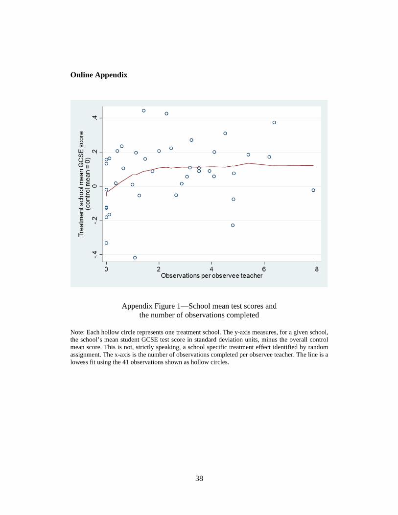
38

Online Appendix

Appendix Figure 1—School mean test scores and the number of observations completed

Note: Each hollow circle represents one treatment school. The y-axis measures, for a given school, the school’s mean student GCSE test score in standard deviation units, minus the overall control mean score. This is not, strictly speaking, a school specific treatment effect identified by random assignment. The x-axis is the number of observations completed per observee teacher. The line is a lowess fit using the 41 observations shown as hollow circles.

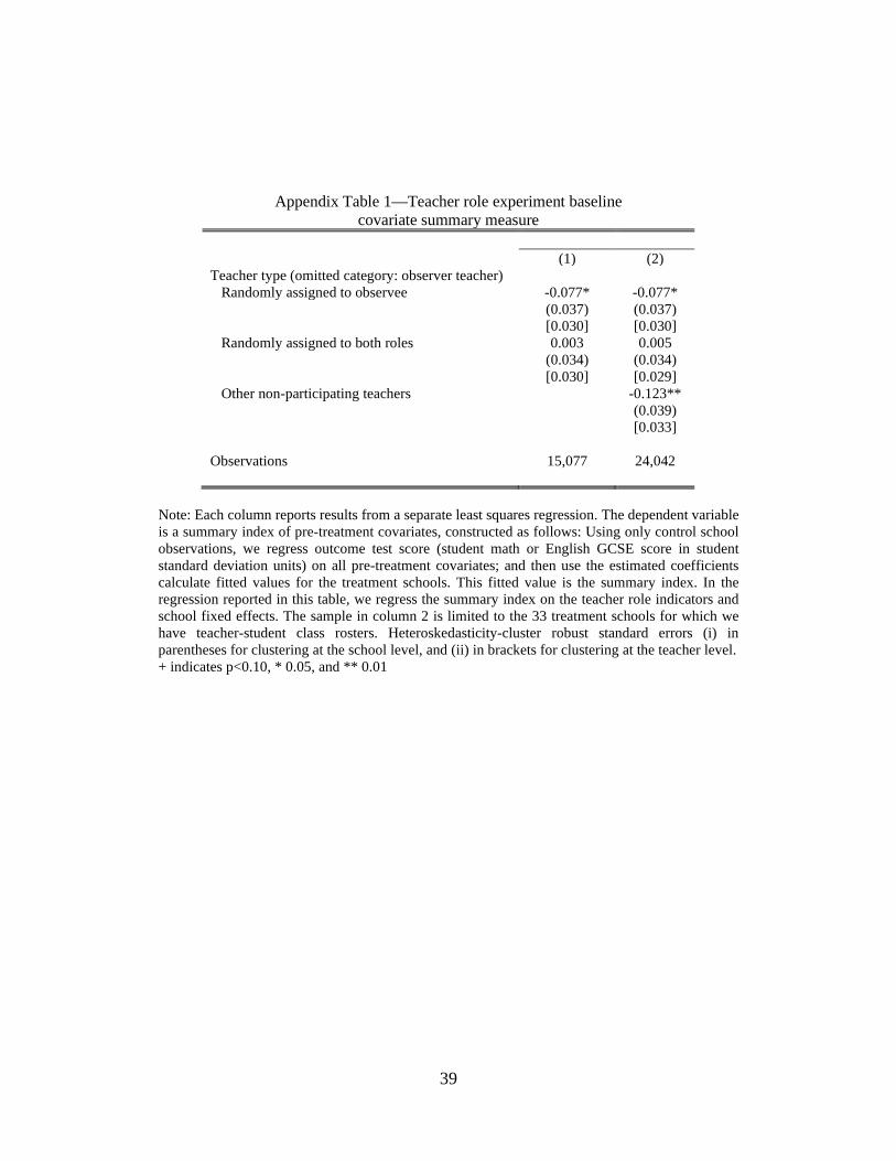
39

Appendix Table 1—Teacher role experiment baseline covariate summary measure (1) (2)

Teacher type (omitted category: observer teacher) Randomly assigned to observee -0.077* -0.077*

(0.037) (0.037) [0.030] [0.030]

Randomly assigned to both roles 0.003 0.005 (0.034) (0.034) [0.030] [0.029]

Other non-participating teachers -0.123** (0.039) [0.033]

Observations 15,077 24,042

Note: Each column reports results from a separate least squares regression. The dependent variable is a summary index of pre-treatment covariates, constructed as follows: Using only control school observations, we regress outcome test score (student math or English GCSE score in student standard deviation units) on all pre-treatment covariates; and then use the estimated coefficients calculate fitted values for the treatment schools. This fitted value is the summary index. In the regression reported in this table, we regress the summary index on the teacher role indicators and school fixed effects. The sample in column 2 is limited to the 33 treatment schools for which we have teacher-student class rosters. Heteroskedasticity-cluster robust standard errors (i) in parentheses for clustering at the school level, and (ii) in brackets for clustering at the teacher level. + indicates p<0.10, * 0.05, and ** 0.01

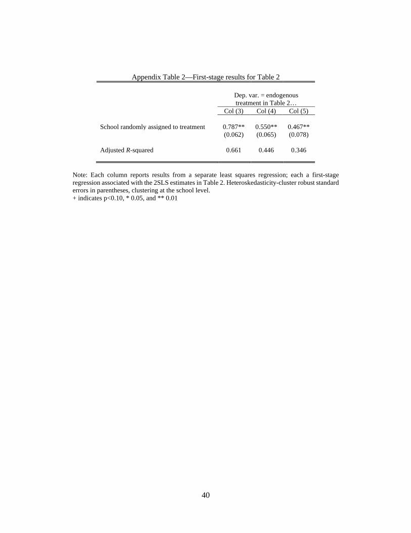
40

Appendix Table 2—First-stage results for Table 2

Dep. var. = endogenous treatment in Table 2…

Col (3) Col (4) Col (5)

School randomly assigned to treatment 0.787** 0.550** 0.467** (0.062) (0.065) (0.078)

Adjusted R-squared 0.661 0.446 0.346

Note: Each column reports results from a separate least squares regression; each a first-stage regression associated with the 2SLS estimates in Table 2. Heteroskedasticity-cluster robust standard errors in parentheses, clustering at the school level. + indicates p<0.10, * 0.05, and ** 0.01

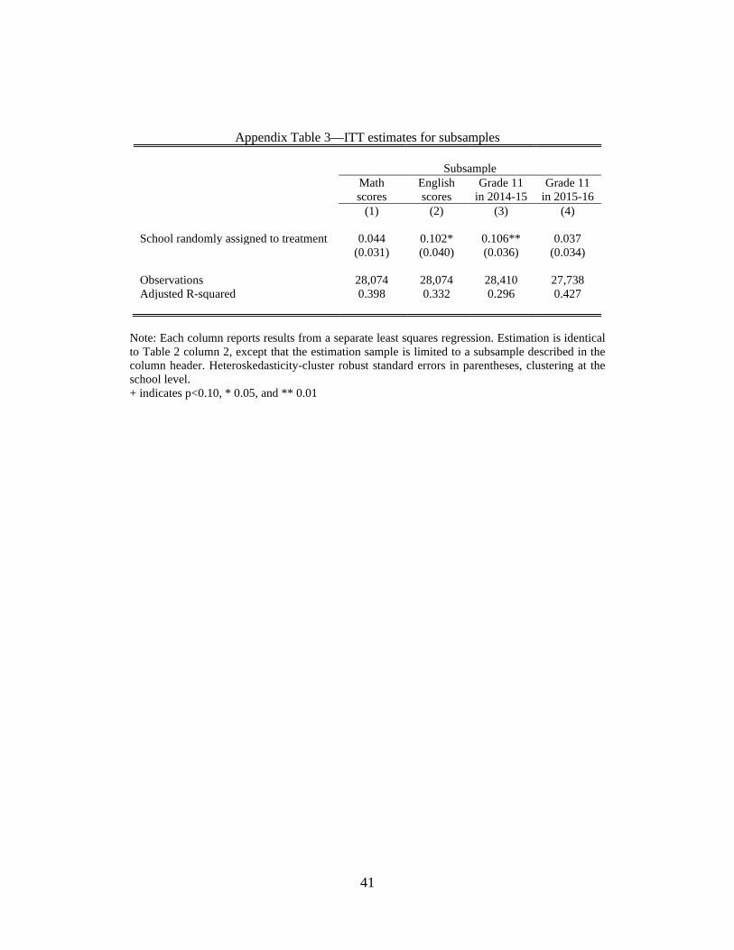
41

Appendix Table 3—ITT estimates for subsamples Subsample

Math scores

English scores

Grade 11 in 2014-15

Grade 11 in 2015-16

(1) (2) (3) (4)

School randomly assigned to treatment 0.044 0.102* 0.106** 0.037 (0.031) (0.040) (0.036) (0.034)

Observations 28,074 28,074 28,410 27,738 Adjusted R-squared 0.398 0.332 0.296 0.427

Note: Each column reports results from a separate least squares regression. Estimation is identical to Table 2 column 2, except that the estimation sample is limited to a subsample described in the column header. Heteroskedasticity-cluster robust standard errors in parentheses, clustering at the school level. + indicates p<0.10, * 0.05, and ** 0.01

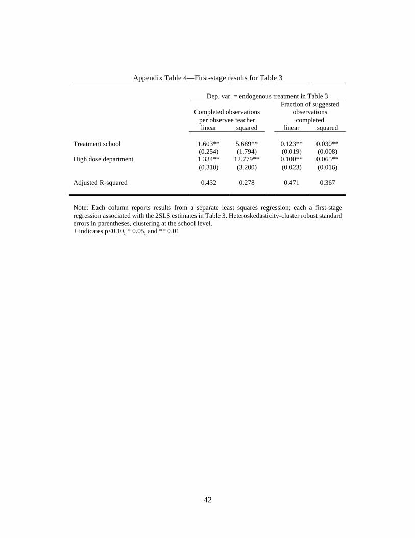
42

Appendix Table 4—First-stage results for Table 3 Dep. var. = endogenous treatment in Table 3

Completed observations

per observee teacher

Fraction of suggested observations completed

linear squared linear squared

Treatment school 1.603** 5.689** 0.123** 0.030** (0.254) (1.794) (0.019) (0.008)

High dose department 1.334** 12.779** 0.100** 0.065** (0.310) (3.200) (0.023) (0.016)

Adjusted R-squared 0.432 0.278 0.471 0.367 Note: Each column reports results from a separate least squares regression; each a first-stage regression associated with the 2SLS estimates in Table 3. Heteroskedasticity-cluster robust standard errors in parentheses, clustering at the school level. + indicates p<0.10, * 0.05, and ** 0.01

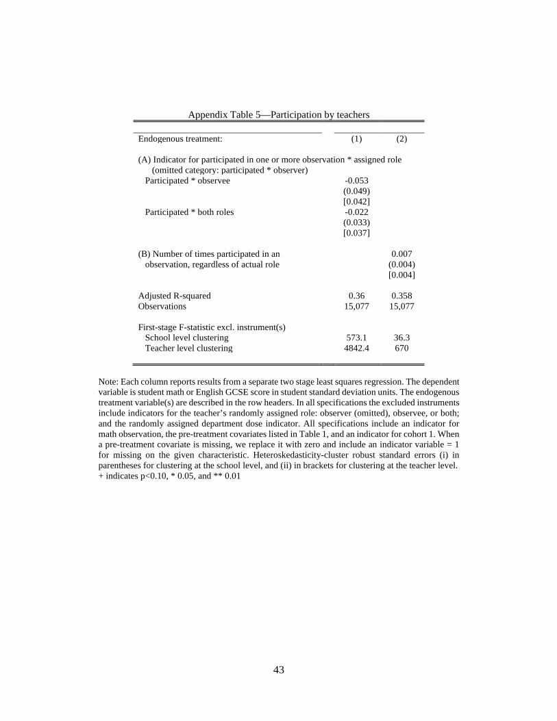
43

Appendix Table 5—Participation by teachers

Endogenous treatment: (1) (2)

(A) Indicator for participated in one or more observation * assigned role (omitted category: participated * observer) Participated * observee -0.053

(0.049) [0.042]

Participated * both roles -0.022 (0.033) [0.037]

(B) Number of times participated in an 0.007 observation, regardless of actual role (0.004)

[0.004]

Adjusted R-squared 0.36 0.358 Observations 15,077 15,077

First-stage F-statistic excl. instrument(s) School level clustering 573.1 36.3 Teacher level clustering 4842.4 670

Note: Each column reports results from a separate two stage least squares regression. The dependent variable is student math or English GCSE score in student standard deviation units. The endogenous treatment variable(s) are described in the row headers. In all specifications the excluded instruments include indicators for the teacher’s randomly assigned role: observer (omitted), observee, or both; and the randomly assigned department dose indicator. All specifications include an indicator for math observation, the pre-treatment covariates listed in Table 1, and an indicator for cohort 1. When a pre-treatment covariate is missing, we replace it with zero and include an indicator variable = 1 for missing on the given characteristic. Heteroskedasticity-cluster robust standard errors (i) in parentheses for clustering at the school level, and (ii) in brackets for clustering at the teacher level. + indicates p<0.10, * 0.05, and ** 0.01

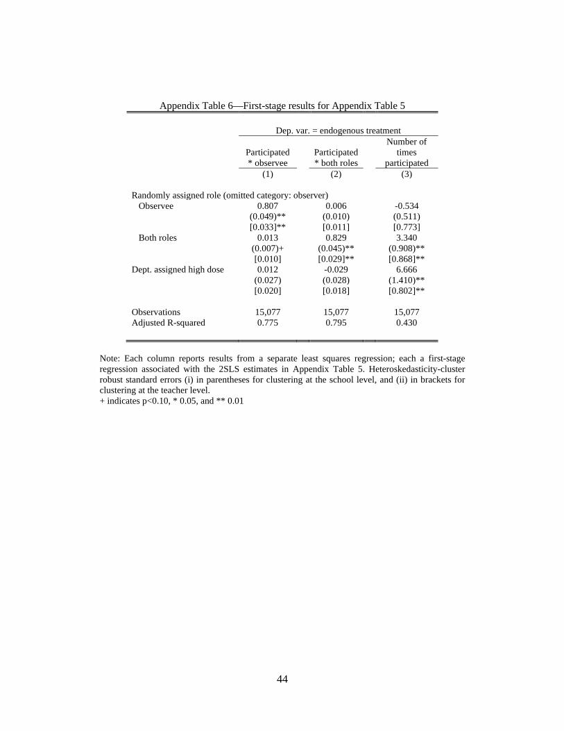
44

Appendix Table 6—First-stage results for Appendix Table 5

Dep. var. = endogenous treatment

Participated * observee

Participated * both roles

Number of times

participated (1) (2) (3)

Randomly assigned role (omitted category: observer) Observee 0.807 0.006 -0.534

(0.049)** (0.010) (0.511) [0.033]** [0.011] [0.773]

Both roles 0.013 0.829 3.340 (0.007)+ (0.045)** (0.908)** [0.010] [0.029]** [0.868]**

Dept. assigned high dose 0.012 -0.029 6.666 (0.027) (0.028) (1.410)** [0.020] [0.018] [0.802]**

Observations 15,077 15,077 15,077 Adjusted R-squared 0.775 0.795 0.430

Note: Each column reports results from a separate least squares regression; each a first-stage regression associated with the 2SLS estimates in Appendix Table 5. Heteroskedasticity-cluster robust standard errors (i) in parentheses for clustering at the school level, and (ii) in brackets for clustering at the teacher level. + indicates p<0.10, * 0.05, and ** 0.01

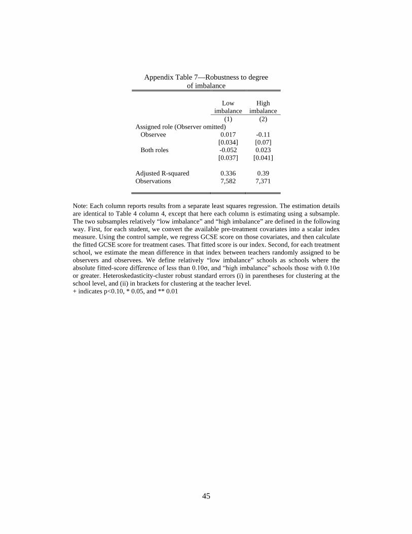
45

Appendix Table 7—Robustness to degree of imbalance

Low

imbalance High

imbalance (1) (2)

Assigned role (Observer omitted) Observee 0.017 -0.11

[0.034] [0.07] Both roles -0.052 0.023

[0.037] [0.041]

Adjusted R-squared 0.336 0.39 Observations 7,582 7,371

Note: Each column reports results from a separate least squares regression. The estimation details are identical to Table 4 column 4, except that here each column is estimating using a subsample. The two subsamples relatively “low imbalance” and “high imbalance” are defined in the following way. First, for each student, we convert the available pre-treatment covariates into a scalar index measure. Using the control sample, we regress GCSE score on those covariates, and then calculate the fitted GCSE score for treatment cases. That fitted score is our index. Second, for each treatment school, we estimate the mean difference in that index between teachers randomly assigned to be observers and observees. We define relatively “low imbalance” schools as schools where the absolute fitted-score difference of less than 0.10σ, and “high imbalance” schools those with 0.10σ or greater. Heteroskedasticity-cluster robust standard errors (i) in parentheses for clustering at the school level, and (ii) in brackets for clustering at the teacher level. + indicates p<0.10, * 0.05, and ** 0.01

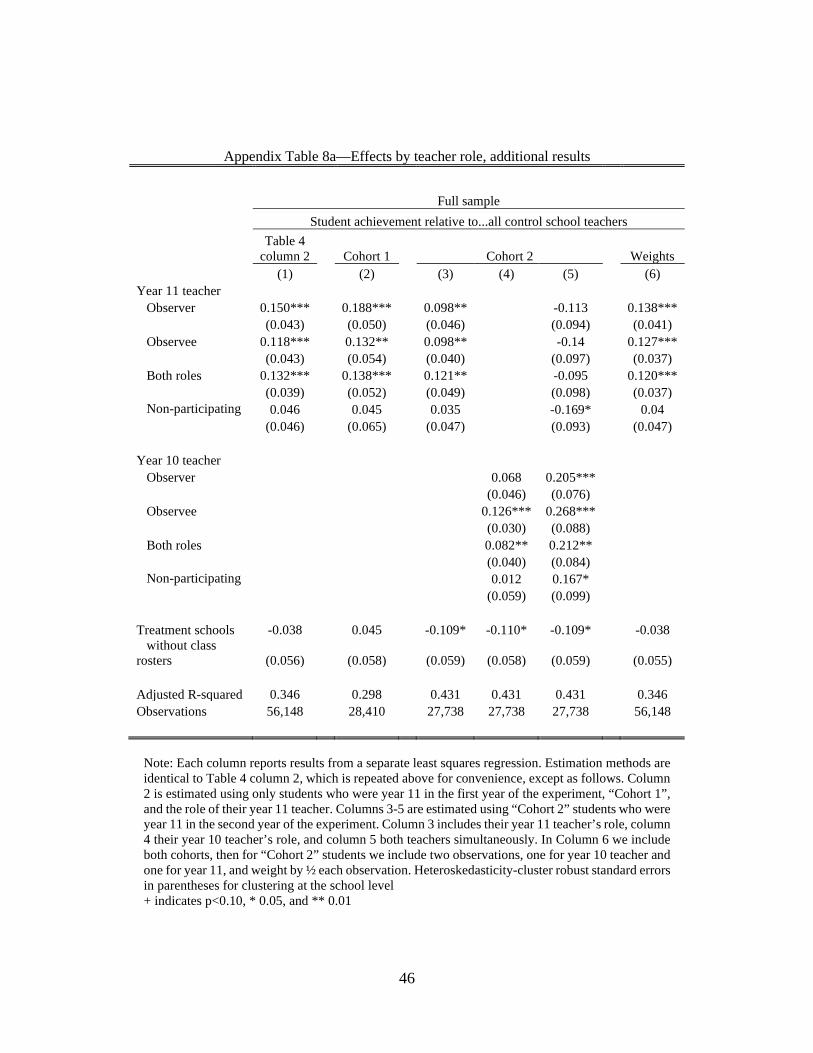
46

Appendix Table 8a—Effects by teacher role, additional results

Full sample

Student achievement relative to...all control school teachers

Table 4

column 2 Cohort 1 Cohort 2 Weights (1) (2) (3) (4) (5) (6)

Year 11 teacher Observer 0.150*** 0.188*** 0.098** -0.113 0.138***

(0.043) (0.050) (0.046) (0.094) (0.041) Observee 0.118*** 0.132** 0.098** -0.14 0.127***

(0.043) (0.054) (0.040) (0.097) (0.037) Both roles 0.132*** 0.138*** 0.121** -0.095 0.120***

(0.039) (0.052) (0.049) (0.098) (0.037) Non-participating 0.046 0.045 0.035 -0.169* 0.04

(0.046) (0.065) (0.047) (0.093) (0.047)

Year 10 teacher Observer 0.068 0.205***

(0.046) (0.076) Observee 0.126*** 0.268***

(0.030) (0.088) Both roles 0.082** 0.212**

(0.040) (0.084) Non-participating 0.012 0.167* (0.059) (0.099)

Treatment schools -0.038 0.045 -0.109* -0.110* -0.109* -0.038 without class rosters (0.056) (0.058) (0.059) (0.058) (0.059) (0.055)

Adjusted R-squared 0.346 0.298 0.431 0.431 0.431 0.346 Observations 56,148 28,410 27,738 27,738 27,738 56,148

Note: Each column reports results from a separate least squares regression. Estimation methods are identical to Table 4 column 2, which is repeated above for convenience, except as follows. Column 2 is estimated using only students who were year 11 in the first year of the experiment, “Cohort 1”, and the role of their year 11 teacher. Columns 3-5 are estimated using “Cohort 2” students who were year 11 in the second year of the experiment. Column 3 includes their year 11 teacher’s role, column 4 their year 10 teacher’s role, and column 5 both teachers simultaneously. In Column 6 we include both cohorts, then for “Cohort 2” students we include two observations, one for year 10 teacher and one for year 11, and weight by ½ each observation. Heteroskedasticity-cluster robust standard errors in parentheses for clustering at the school level + indicates p<0.10, * 0.05, and ** 0.01

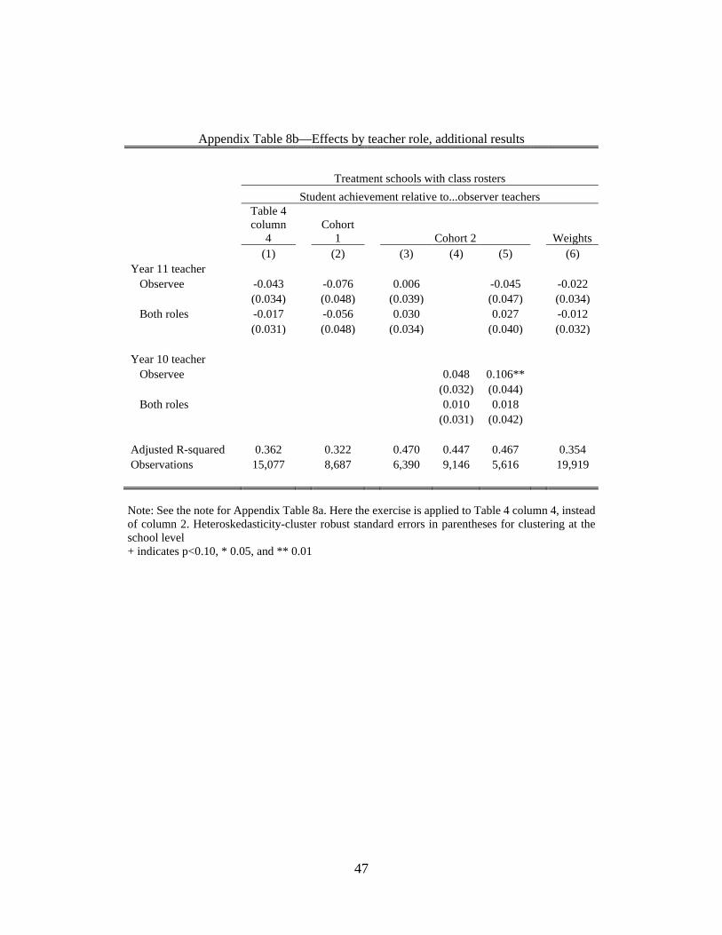
47

Appendix Table 8b—Effects by teacher role, additional results

Treatment schools with class rosters

Student achievement relative to...observer teachers

Table 4 column

4 Cohort

1 Cohort 2 Weights (1) (2) (3) (4) (5) (6)

Year 11 teacher Observee -0.043 -0.076 0.006 -0.045 -0.022

(0.034) (0.048) (0.039) (0.047) (0.034) Both roles -0.017 -0.056 0.030 0.027 -0.012

(0.031) (0.048) (0.034) (0.040) (0.032)

Year 10 teacher Observee 0.048 0.106**

(0.032) (0.044) Both roles 0.010 0.018 (0.031) (0.042) Adjusted R-squared 0.362 0.322 0.470 0.447 0.467 0.354 Observations 15,077 8,687 6,390 9,146 5,616 19,919

Note: See the note for Appendix Table 8a. Here the exercise is applied to Table 4 column 4, instead of column 2. Heteroskedasticity-cluster robust standard errors in parentheses for clustering at the school level + indicates p<0.10, * 0.05, and ** 0.01

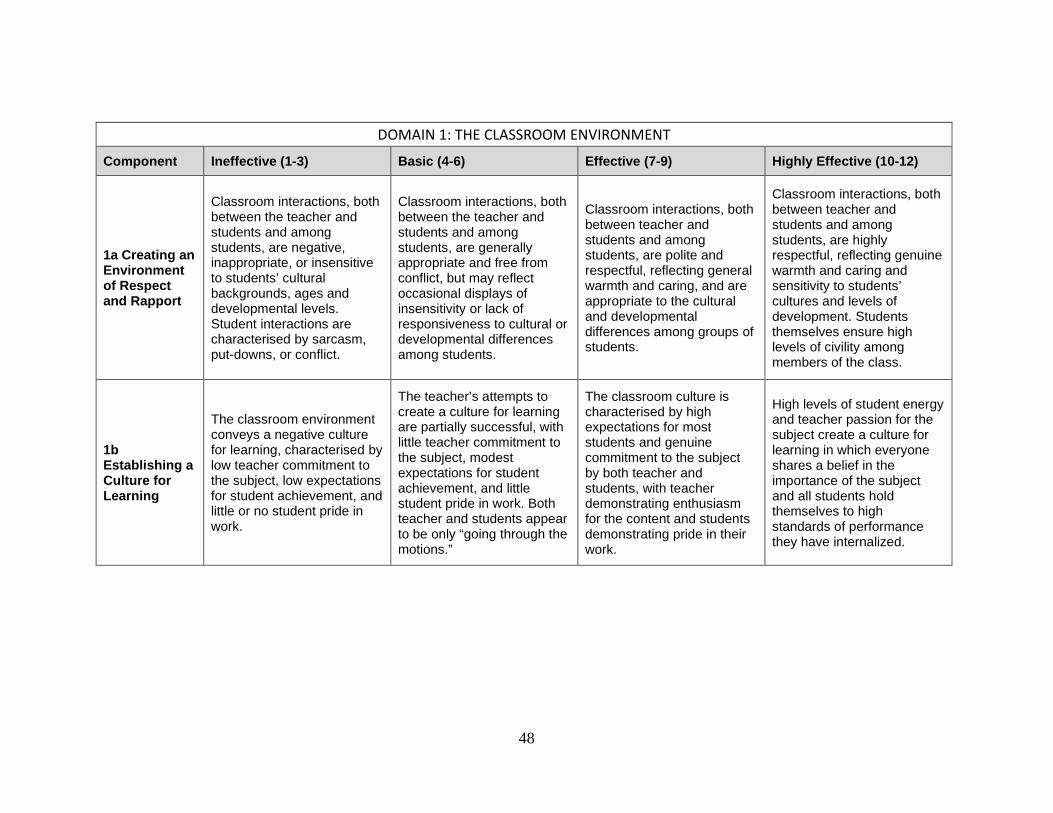
48

DOMAIN 1: THE CLASSROOM ENVIRONMENT

Component Ineffective (1-3) Basic (4-6) Effective (7-9) Highly Effective (10-12)

1a Creating an Environment of Respect and Rapport

Classroom interactions, both between the teacher and students and among students, are negative, inappropriate, or insensitive to students’ cultural backgrounds, ages and developmental levels. Student interactions are characterised by sarcasm, put-downs, or conflict.

Classroom interactions, both between the teacher and students and among students, are generally appropriate and free from conflict, but may reflect occasional displays of insensitivity or lack of responsiveness to cultural or developmental differences among students.

Classroom interactions, both between teacher and students and among students, are polite and respectful, reflecting general warmth and caring, and are appropriate to the cultural and developmental differences among groups of students.

Classroom interactions, both between teacher and students and among students, are highly respectful, reflecting genuine warmth and caring and sensitivity to students’ cultures and levels of development. Students themselves ensure high levels of civility among members of the class.

1b Establishing a Culture for Learning

The classroom environment conveys a negative culture for learning, characterised by low teacher commitment to the subject, low expectations for student achievement, and little or no student pride in work.

The teacher’s attempts to create a culture for learning are partially successful, with little teacher commitment to the subject, modest expectations for student achievement, and little student pride in work. Both teacher and students appear to be only “going through the motions.”

The classroom culture is characterised by high expectations for most students and genuine commitment to the subject by both teacher and students, with teacher demonstrating enthusiasm for the content and students demonstrating pride in their work.

High levels of student energy and teacher passion for the subject create a culture for learning in which everyone shares a belief in the importance of the subject and all students hold themselves to high standards of performance they have internalized.

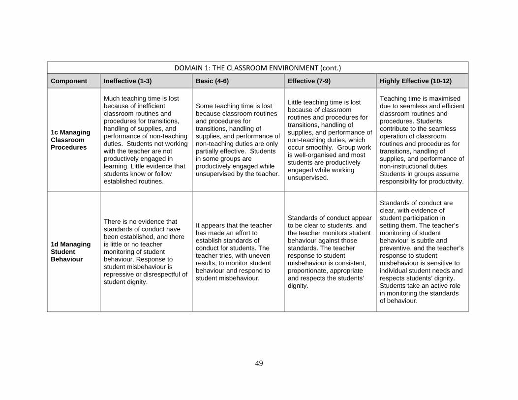
49

DOMAIN 1: THE CLASSROOM ENVIRONMENT (cont.)

Component Ineffective (1-3) Basic (4-6) Effective (7-9) Highly Effective (10-12)

1c Managing Classroom Procedures

Much teaching time is lost because of inefficient classroom routines and procedures for transitions, handling of supplies, and performance of non-teaching duties. Students not working with the teacher are not productively engaged in learning. Little evidence that students know or follow established routines.

Some teaching time is lost because classroom routines and procedures for transitions, handling of supplies, and performance of non-teaching duties are only partially effective. Students in some groups are productively engaged while unsupervised by the teacher.

Little teaching time is lost because of classroom routines and procedures for transitions, handling of supplies, and performance of non-teaching duties, which occur smoothly. Group work is well-organised and most students are productively engaged while working unsupervised.

Teaching time is maximised due to seamless and efficient classroom routines and procedures. Students contribute to the seamless operation of classroom routines and procedures for transitions, handling of supplies, and performance of non-instructional duties. Students in groups assume responsibility for productivity.

1d Managing Student Behaviour

There is no evidence that standards of conduct have been established, and there is little or no teacher monitoring of student behaviour. Response to student misbehaviour is repressive or disrespectful of student dignity.

It appears that the teacher has made an effort to establish standards of conduct for students. The teacher tries, with uneven results, to monitor student behaviour and respond to student misbehaviour.

Standards of conduct appear to be clear to students, and the teacher monitors student behaviour against those standards. The teacher response to student misbehaviour is consistent, proportionate, appropriate and respects the students’ dignity.

Standards of conduct are clear, with evidence of student participation in setting them. The teacher’s monitoring of student behaviour is subtle and preventive, and the teacher’s response to student misbehaviour is sensitive to individual student needs and respects students’ dignity. Students take an active role in monitoring the standards of behaviour.

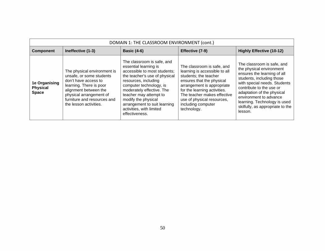
50

DOMAIN 1: THE CLASSROOM ENVIRONMENT (cont.)

Component Ineffective (1-3) Basic (4-6) Effective (7-9) Highly Effective (10-12)

1e Organising Physical Space

The physical environment is unsafe, or some students don’t have access to learning. There is poor alignment between the physical arrangement of furniture and resources and the lesson activities.

The classroom is safe, and essential learning is accessible to most students; the teacher’s use of physical resources, including computer technology, is moderately effective. The teacher may attempt to modify the physical arrangement to suit learning activities, with limited effectiveness.

The classroom is safe, and learning is accessible to all students; the teacher ensures that the physical arrangement is appropriate for the learning activities. The teacher makes effective use of physical resources, including computer technology.

The classroom is safe, and the physical environment ensures the learning of all students, including those with special needs. Students contribute to the use or adaptation of the physical environment to advance learning. Technology is used skilfully, as appropriate to the lesson.

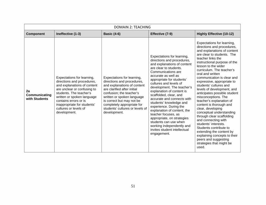
51

DOMAIN 2: TEACHING

Component Ineffective (1-3) Basic (4-6) Effective (7-9) Highly Effective (10-12)

2a Communicating with Students

Expectations for learning, directions and procedures, and explanations of content are unclear or confusing to students. The teacher’s written or spoken language contains errors or is inappropriate for students’ cultures or levels of development.

Expectations for learning, directions and procedures, and explanations of content are clarified after initial confusion; the teacher’s written or spoken language is correct but may not be completely appropriate for students’ cultures or levels of development.

Expectations for learning, directions and procedures, and explanations of content are clear to students. Communications are accurate as well as appropriate for students’ cultures and levels of development. The teacher’s explanation of content is scaffolded, clear, and accurate and connects with students’ knowledge and experience. During the explanation of content, the teacher focuses, as appropriate, on strategies students can use when working independently and invites student intellectual engagement.

Expectations for learning, directions and procedures, and explanations of content are clear to students. The teacher links the instructional purpose of the lesson to the wider curriculum. The teacher’s oral and written communication is clear and expressive, appropriate to students’ cultures and levels of development, and anticipates possible student misconceptions. The teacher’s explanation of content is thorough and clear, developing conceptual understanding through clear scaffolding and connecting with students’ interests. Students contribute to extending the content by explaining concepts to their peers and suggesting strategies that might be used.

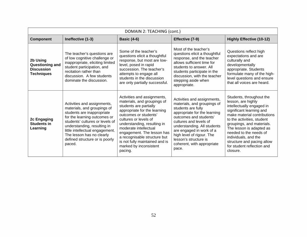
52

DOMAIN 2: TEACHING (cont.)

Component Ineffective (1-3) Basic (4-6) Effective (7-9) Highly Effective (10-12)

2b Using Questioning and Discussion Techniques

The teacher’s questions are of low cognitive challenge or inappropriate, eliciting limited student participation, and recitation rather than discussion. A few students dominate the discussion.

Some of the teacher’s questions elicit a thoughtful response, but most are low-level, posed in rapid succession. The teacher’s attempts to engage all students in the discussion are only partially successful.

Most of the teacher’s questions elicit a thoughtful response, and the teacher allows sufficient time for students to answer. All students participate in the discussion, with the teacher stepping aside when appropriate.

Questions reflect high expectations and are culturally and developmentally appropriate. Students formulate many of the high-level questions and ensure that all voices are heard.

2c Engaging Students in Learning

Activities and assignments, materials, and groupings of students are inappropriate for the learning outcomes or students’ cultures or levels of understanding, resulting in little intellectual engagement. The lesson has no clearly defined structure or is poorly paced.

Activities and assignments, materials, and groupings of students are partially appropriate for the learning outcomes or students’ cultures or levels of understanding, resulting in moderate intellectual engagement. The lesson has a recognisable structure but is not fully maintained and is marked by inconsistent pacing.

Activities and assignments, materials, and groupings of students are fully appropriate for the learning outcomes and students’ cultures and levels of understanding. All students are engaged in work of a high level of rigour. The lesson’s structure is coherent, with appropriate pace.

Students, throughout the lesson, are highly intellectually engaged in significant learning and make material contributions to the activities, student groupings, and materials. The lesson is adapted as needed to the needs of individuals, and the structure and pacing allow for student reflection and closure.

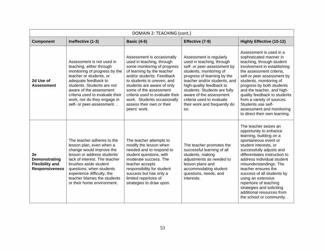
53

DOMAIN 2: TEACHING (cont.)

Component Ineffective (1-3) Basic (4-6) Effective (7-9) Highly Effective (10-12)

2d Use of Assessment

Assessment is not used in teaching, either through monitoring of progress by the teacher or students, or adequate feedback to students. Students are not aware of the assessment criteria used to evaluate their work, nor do they engage in self- or peer-assessment. .

Assessment is occasionally used in teaching, through some monitoring of progress of learning by the teacher and/or students. Feedback to students is uneven, and students are aware of only some of the assessment criteria used to evaluate their work. Students occasionally assess their own or their peers’ work.

Assessment is regularly used in teaching, through self- or peer-assessment by students, monitoring of progress of learning by the teacher and/or students, and high-quality feedback to students. Students are fully aware of the assessment criteria used to evaluate their work and frequently do so.

Assessment is used in a sophisticated manner in teaching, through student involvement in establishing the assessment criteria, self-or peer assessment by students, monitoring of progress by both students and the teacher, and high-quality feedback to students from a variety of sources. Students use self-assessment and monitoring to direct their own learning.

2e Demonstrating Flexibility and Responsiveness

The teacher adheres to the lesson plan, even when a change would improve the lesson or address students’ lack of interest. The teacher brushes aside student questions; when students experience difficulty, the teacher blames the students or their home environment.

The teacher attempts to modify the lesson when needed and to respond to student questions, with moderate success. The teacher accepts responsibility for student success but has only a limited repertoire of strategies to draw upon.

The teacher promotes the successful learning of all students, making adjustments as needed to lesson plans and accommodating student questions, needs, and interests.

The teacher seizes an opportunity to enhance learning, building on a spontaneous event or student interests, or successfully adjusts and differentiates instruction to address individual student misunderstandings. The teacher ensures the success of all students by using an extensive repertoire of teaching strategies and soliciting additional resources from the school or community. .