taming epidemic outbreaks in mobile adhoc networks
TRANSCRIPT
Ad Hoc Networks 24 (2015) 57–72
Contents lists available at ScienceDirect
Ad Hoc Networks
journal homepage: www.elsevier .com/locate /adhoc
Taming epidemic outbreaks in mobile adhoc networks q
http://dx.doi.org/10.1016/j.adhoc.2014.07.0311570-8705/� 2014 Elsevier B.V. All rights reserved.
q Parts of this work were presented at the 2012 IEEE Conference onMobile Adhoc and Sensor Systems (MASS) [1] as a regular paper.⇑ Corresponding authors.
E-mail addresses: [email protected] (E. Hoque), [email protected] (R. Potharaju), [email protected] (C. Nita-Rotaru), [email protected] (S. Sarkar), [email protected] (S.S. Venkatesh).
E. Hoque a,⇑, R. Potharaju a,*, C. Nita-Rotaru a, S. Sarkar b, S.S. Venkatesh b
a Department of Computer Science, Purdue University, West Lafayette, IN, USAb Department of Electrical Engineering, University of Pennsylvania, Philadelphia, PA, USA
a r t i c l e i n f o a b s t r a c t
Article history:Received 25 June 2013Received in revised form 6 May 2014Accepted 28 July 2014Available online 19 August 2014
Keywords:EpidemicMalwareDefenseMobile adhoc networks
The openness of the smartphone operating systems has increased the number of applica-tions developed, but it has also introduced a new propagation vector for mobile malware.We model the propagation of mobile malware among humans carrying smartphones usingepidemiology theory and study the problem as a function of the underlying mobility mod-els. We define the optimal approach to heal an infected system with the help of a set ofstatic healers that distribute patches as the T-COVER problem, which is NP-COMPLETE. We thenpropose three families of healer protocols that allow for a trade-off between the recoverytime and the energy consumed for deploying patches. We show through simulations usingthe NS-3 simulator that despite lacking knowledge of the exact future, our healers obtain arecovery time within a 7.4� � 10� bound of the oracle solution that has knowledge of thefuture arrival time of all the infected nodes.
� 2014 Elsevier B.V. All rights reserved.
1. Introduction
With the advent of Google’s Android, the number of wire-less devices with complex capabilities and the support toopen source operating systems has significantly increased.While the openness of operating systems induces develop-ers’ motivation, it also introduces a new propagation vectorfor mobile malware. Recent reports show a significantincrease in malware targeting Android devices [2,3].
Significant research focused on propagation modeling,detection, and application profiling of malware in the con-text of wired networks [4–8]. Those results do not modelmobile malware which spreads directly from device todevice by using short-range communication such as WiFi,Bluetooth or NFC [9–12]. Mobile malware propagation
has been studied using mean field compartmental models[13] which assume that each infected node will contactevery neighbor once within one time step, i.e., the infectiv-ity is equal to the connectivity. Such models do not takeinto account that mobile malware does not spread at aneven contact rate, as spreading requires devices to bewithin each other’s proximity which in turn depends onuser mobility. Most previous research on mobile malwarehas either not considered mobility [14–16] or has givenlimited considerations to it [17,18]. Approaches that haveconsidered mobility have used popular models like therandom waypoint model which, as it has been shown, doesnot realistically mimic human mobility [19].
While there has been work studying mobile malwarepropagation, the problem of infection containment in wire-less networks was less studied. The work of [20] analyti-cally studies containment of infection in a mobilenetwork through countermeasures such as reducingcommunication range of nodes during an infectionoutbreak. The work does not consider realistic mobilitymodels and does not propose concrete protocols to deployand activate such countermeasures. The work in [21]
0
200
400
600
800
1000
0 200 400 600 800 1000
Y
X
Random Waypoint
0
200
400
600
800
1000
0 200 400 600 800 1000
Y
X
Truncated Levy Walk
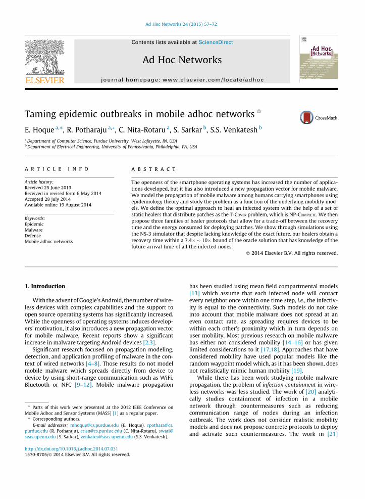
Fig. 1. (a) and (b) Tracing the path of a single node for RWP and TLW: Observe the short paths in RWP and bursty long paths in TLW.
58 E. Hoque et al. / Ad Hoc Networks 24 (2015) 57–72
introduces replicative and non-replicative patch dissemi-nations assuming a network cost function and proves thatthe dynamic control strategies have a simple optimalstructure. However, the impractical determination of thehealer activation time and the lack of inclusion of theresource cost incurred by each patch dissemination makethe techniques difficult to apply directly to energy con-strained realistic scenarios.
In this paper, we take the first step towards designingcountermeasures for malware propagation under the pres-ence of realistic mobility in a practical scenario. We investi-gate the dependence of infection spread on the underlyingmobility model in order to systematize the design of coun-termeasures. We introduce the concept of healers to mimicthe recovery process in a standard epidemic model and wefocus on static healers, i.e., immobile healers, which repre-sent a realistic model because they can be directly mappedto real-world scenarios. For instance, static healers can beconsidered as cellular base stations (where no two stationscover the same cell in most cases) and the mobile nodes canbe considered as users carrying mobile phones (movingwith a certain mobility model). Unlike [17], our static-heal-ers are not white-worms and do not deactivate infectednodes. Our contributions are:
� We show that the infection spread in mobility models thatmimic human behavior is slower than standard mobilitymodels due to different contact rate and spatial distribu-tion characteristics. We compare the Truncated LevyWalk (TLW) and Random Waypoint (RWP) mobility mod-els and show that the epidemic spread in TLW is relativelyslower compared to RWP. This finding indicates that whendesigning countermeasure mechanisms, the time con-straints are less tight than believed and that time-depen-dent assumptions can be relaxed to some extent, resultingin relatively lower consumption of energy.� We model countermeasures to malware spread using
static healer nodes. Static healers once placed in thearea, act independently to deploy a patch when theysense nodes in their proximity. A healer-based solutionoptimizes: (i) the time it takes to heal the entire system
by patching all the infected nodes and (ii) the totalnumber of patches broadcasted. We formulate the opti-mal solution based on static healers as a T-COVER prob-lem, which is NP-COMPLETE.� We use ORACLE, a logðnÞ greedy approximation algo-
rithm, that computes the optimal healing time knowingthe placement of the static healers and the future, i.e. theexact time instances when the infected nodes arrivewithin each healer’s proximity.� We propose a novel healer placement strategy using
blue-noise distribution generating Poisson Disk Sam-pling. We show that unlike random placement thatresults in many overlapping healers which cover thesame area, our method allows healers to cover disjointareas, thus enabling them to independently cover moreinfected nodes.� We design three families of healer protocols: randomized
(RH), profile (PH), and prediction (PDH ), that allow for atrade-off between the energy consumed for sendingpatches and the time taken to recover the entire system.The intuition behind each protocol is as follows: (1) RHuses randomization to ensure simplicity in healers’ func-tionality and achieves reasonable performance. (2) PHuses system feedback to optimize the energy consumedfor sending patches, but may result in a larger recoverytime. (3) PDH predicts the cost of waiting for a suitabletime instance to deploy a patch thereby achieving a smal-ler recovery time but has the side-effect of utilizing morepatches. We compare our protocols with the ORACLEprotocol and show through simulations that despitelacking knowledge of the future, our healers obtain arecovery time within a 7.4� � 10�bound of the ORACLE.
The rest of this paper is organized as follows. Section 2describes our system model, our assumptions and intro-duces the mobility models used in this paper. Section 3analyzes the infection dynamics as a function of the under-lying mobility models. Section 4 introduces our healer-based protocols and Section 5 provides simulation results.Section 6 discusses related research and Section 7 con-cludes the paper.
E. Hoque et al. / Ad Hoc Networks 24 (2015) 57–72 59
2. System model
In this section, we construct a framework for analyzingthe propagation of malware over a mobile ad hoc networkthat relies on epidemic theory to capture both the spatialinteraction of nodes and the temporal dynamics of infec-tion propagation.
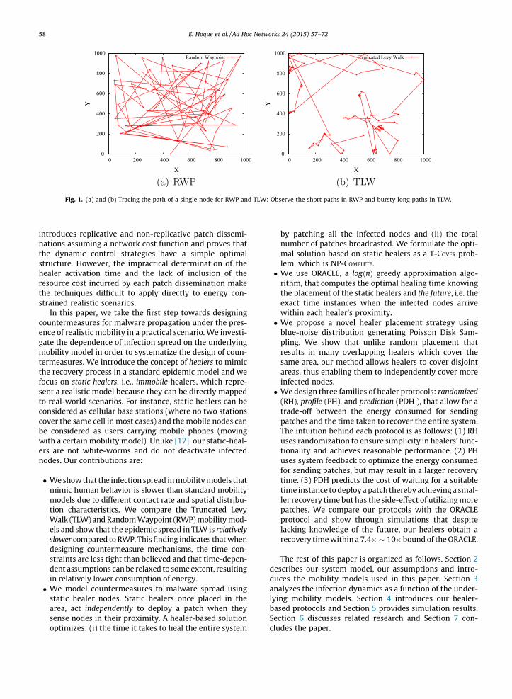
Fig. 2. SIR Model: S, susceptible; I, infected; R, recovered.
2.1. Mobility models
Due to the difficulties in adapting real-trace data to longrunning simulations [16], we decided to use analyticalmodels derived from real-trace data instead. Specifically,we use the Random Waypoint (RWP) and Truncated Levywalk (TLW) mobility models to generate synthetic mobilitytraces. We selected RWP because it is a typical mobilitymodel used to study mobile malware propagation. Weselected TLW because it provides more realistic represen-tations of statistical patterns found in human mobility.Unless otherwise noted, we use a node velocity of 0.6 m/s to mimic low velocity realistic human mobility in bothmobility models throughout the paper.
Random Waypoint (RWP): RWP is a widely used mobil-ity model [22–24] and includes pause times betweenchanges in direction and/or speed [25]. A mobile nodebegins by staying in one location for a certain time period(pause time). Once this time elapses, the mobile nodechooses a random destination in the simulation area anda speed that is uniformly distributed between ½vmin;vmax�.The mobile node then travels toward the newly chosendestination at the selected speed. Upon arrival, the nodepauses for a specified time period and starts the whole pro-cess again (see Fig. 1(a)). RWP is heavily used for mobile adhoc network simulation [26] to simulate mobile nodes thatcan move randomly and freely in a mobility area withoutany restriction. This model is super-diffusive because ofhigh-probability of long flights. On the contrary, humanwalks have heavy-tail flight distributions [27] that arenot captured by common mobility models such as RWP.
The initial random distribution of mobile nodes is notrepresentative of the manner in which nodes distributethemselves when moving as the instantaneous mobilenode neighbor percentage possess high variability [28].We use the approach suggested by [26] and discard the ini-tial 1000 s of simulation time produced by RWP in eachsimulation trial.
Truncated Levy Walk (TLW): Based on the empiricalstudies performed on human mobility data collectedthrough mobile devices carried by humans, Rhee et al.[19] reported that human walks performed in outdoor set-tings of tens of kilometers resemble a truncated form ofLevy walks commonly observed in animals such as spidermonkeys, birds and jackals. A Levy walk is a type of randomwalk in which the increments are distributed according toa heavy-tailed probability distribution, i.e., their tails arenot exponentially bounded. The distribution used is apower law of the form y ¼ x�a where 1 < a < 3. TLW is arandom equivalent mobility model for human walksin that it can describe some important characteristicsof human walks (e.g. flight length, pause time and
inter-contact time) despite being a random model. Inter-contact times are defined to be the time durations betweentwo consecutive meeting events of the same two nodes.Human walks have long inter-contact times, which is intu-itive in a sense that as humans do not move much, theywill not meet each other very often. The distributions ofthese inter-contact times, which follows a power-law dis-tribution with an exponential tail, are similar to thoseobserved in case of Levy walks. Similarly, the heavy-taildistributions of flight length and pause time can be cap-tured by Levy walkers moving in a confined area. Intui-tively, Levy walks consist of many short flights andexceptionally long flights that nullify the effect of suchshort flights (see Fig. 1(b)).
Note that while there are other recent human mobilitymodels similar to TLW such as the ones proposed by Leeet al. [29], Boldrini et al. [30] and Isaacman et al. [31],our end goal is to advocate the use of one of thesehuman mobility models while designing defenses againstepidemic outbreaks.
2.2. Infection and recovery models
We adapt two classic epidemic models (SI and SIR) totake into account mobility. First we give a brief overviewof the SI and SIR models, then describe how we use themto model malware propagation and node recovery in amobile network.
SI Model. The SI-model is a two-state compartmentalepidemic model, i.e., a node can stay in one of two states:susceptible and infected. A susceptible node is vulnerableand can be exploited to be infected which in turn can infectother susceptible nodes. In this model, once a susceptiblenode is infected, it stays that way. The parameter thatcharacterizes the model is the infection rate, b.
SIR Model. The SIR Kermack–McKendrick model [32]assumes that an infected node can be recovered. Specifi-cally a node can be in one of the following states: suscepti-ble, infected, and recovered. Nodes flow from thesusceptible group to the infected group and then to therecovered group [33] as shown in Fig. 2. The model ischaracterized by two parameters, the infection rate b andthe recovery rate a.
Mobile Infection Model. The SI model makes the unreal-istic assumption that each infected node will contact everyneighbor once within one time step, i.e., the infectivity isequal to the connectivity. To take into account mobility,we assume the nodes are moving according with a mobil-ity model and we define infection spread as a function of aparameter c which we call the probability of successful
0
0.2
0.4
0.6
0.8
0 1000 2000 3000 4000 5000 6000 7000 8000
Time (sec)
Frac
tion
of m
obile
nod
es
RWP mobility modelSusceptible: 100 nodes
Infected: 100 nodesSusceptible: 200 nodes
Infected: 200 nodesSusceptible: 300 nodes
Infected: 300 nodes
0
0.2
0.4
0.6
0.8
1TLW mobility model
Susceptible: 100 nodesInfected: 100 nodes
Susceptible: 200 nodesInfected: 200 nodes
Susceptible: 300 nodesInfected: 300 nodes
0 0.2 0.4 0.6 0.8
1
0 0.2 0.4 0.6 0.8 1
Contacts per second
CD
F
RWP mobility model
100 nodes200 nodes300 nodes
0
0.2
0.4
0.6
0.8
1
1.2
TLW mobility model
100 nodes200 nodes300 nodes
(a) (b)
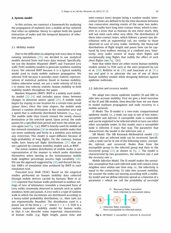
Fig. 3. (a) Inversion point in RWP and TLW: Observe that the infection spread is slower in TLW. (b) Explaining the slow propagation: Observe the contactrate in TLW which is less than RWP.
60 E. Hoque et al. / Ad Hoc Networks 24 (2015) 57–72
transmission. At each time step, for every node X, we findthe neighbors of X that are capable of infecting X. For eachof these neighbors, we generate a random number from auniform distribution between ½0;1� and if this value issmaller than c, then X becomes infected.
Mobile Recovery Model. We adapt the SIR epidemicmodel as follows. Infection is modeled as in the mobileinfection model above. We map node recovery through ahealer that will change the state of an infected node torecovered through a healing mechanism. Once recovered,a node can no longer be infected, thus if no new nodesare added the infection will eventually disappear. The heal-ing mechanism is distributed through a patch, a healer cansend at most once during an interval of time called epoch,denoted as s. We assume that healers are static, resourceconstrained, and act independently. Our assumptions alsoinclude that once an infected node receives a patch, thenode instantaneously applies the patch and becomes com-pletely recovered. We assume that there is no packet lossbut note that it is straightforward to extend our model toa model having packet loss.
This model is characterized by the way the healers areplaced and by the frequency with which they send patches.All healers are activated once the number of infected nodesin the system reached a system-wide parameter.
3. Infection dynamics
In order to understand the infection dynamics of thetwo mobility models, we first describe our methodologyand then explain the results that we observed.
3.1. Methodology
We use the infection model described in previous sec-tion with the parameter that controls the infection rate,c ¼ 0:3 [34] to mimic a more realistic infection scenariowhere infection spreads slowly. We generate RWP tracesby using the methodology outlined in [35] and TLW tracesby using the algorithm outlined in [19]. We perform oursimulations using NS-3 [36]. We simulate the behavior of
a system with 100, 200, and 300 nodes in a fixed area.All results have been averaged over ten simulation runs.
We define an inversion point to be the time instantwhere 50% of the population is infected. We use this metricto indicate the first point in time where the number ofinfected nodes surpasses the susceptible ones, thus invert-ing the scenario. Intuitively, an inversion point character-izes how fast the infection is propagating in an epidemicsystem.
3.2. Results
Fig. 3 shows the infection dynamics in RWP and TLWmobility models. Observe that the inversion point forRWP occurs quite early in the simulation (Fig. 3(a) indi-cates a time around 500 s) in comparison with TLW(Fig. 3(a) indicates times between 1500–3000 s). This indi-cates that the time required to infect the system is far lessin case of RWP differing almost by a factor of 3 from TLW.To the best of our knowledge, this phenomenon has notbeen observed before as most earlier research [17,18] hasstudied these mobility models in isolation. As protocolsare to be designed mostly for realistic mobility models(TLW in this case), this comes as a good news in that cer-tain assumptions such as time-constrained-ness of a proto-col can be relaxed to some extent, resulting in relativelylower consumption of energy.
We gain insights into the reasons behind the slow infec-tion propagation for TLW by using two metrics: (i) contactrate and (ii) spatial distributions of node mobility.
1. Contact Rate: Contact rate is the average number ofnodes encountered by any given node over the duration ofsimulation. We plot an empirical cumulative distributioncurve (ECDF) of the contact rate in Fig. 3(b) for RWP andTLW. Observe that the median contact rate of nodes in caseof RWP is almost always higher than that in TLW. The sameeffect can be observed for the 95th percentile indicatingthat in RWP, a given node comes in contact with a rela-tively higher number of nodes thereby increasing itschances of infecting other nodes or getting infected byother infected nodes.
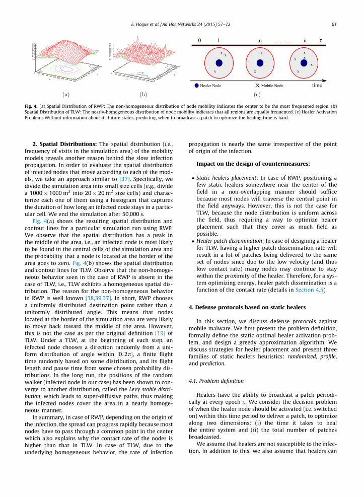
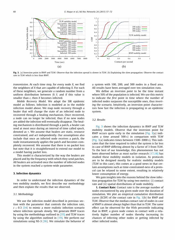
Fig. 4. (a) Spatial Distribution of RWP: The non-homogeneous distribution of node mobility indicates the center to be the most frequented region. (b)Spatial Distribution of TLW: The nearly-homogeneous distribution of node mobility indicates that all regions are equally frequented. (c) Healer ActivationProblem: Without information about its future states, predicting when to broadcast a patch to optimize the healing time is hard.
E. Hoque et al. / Ad Hoc Networks 24 (2015) 57–72 61
2. Spatial Distributions: The spatial distribution (i.e.,frequency of visits in the simulation area) of the mobilitymodels reveals another reason behind the slow infectionpropagation. In order to evaluate the spatial distributionof infected nodes that move according to each of the mod-els, we take an approach similar to [37]. Specifically, wedivide the simulation area into small size cells (e.g., dividea 1000 � 1000 m2 into 20 � 20 m2 size cells) and charac-terize each one of them using a histogram that capturesthe duration of how long an infected node stays in a partic-ular cell. We end the simulation after 50,000 s.
Fig. 4(a) shows the resulting spatial distribution andcontour lines for a particular simulation run using RWP.We observe that the spatial distribution has a peak inthe middle of the area, i.e., an infected node is most likelyto be found in the central cells of the simulation area andthe probability that a node is located at the border of thearea goes to zero. Fig. 4(b) shows the spatial distributionand contour lines for TLW. Observe that the non-homoge-neous behavior seen in the case of RWP is absent in thecase of TLW, i.e., TLW exhibits a homogeneous spatial dis-tribution. The reason for the non-homogeneous behaviorin RWP is well known [38,39,37]. In short, RWP choosesa uniformly distributed destination point rather than auniformly distributed angle. This means that nodeslocated at the border of the simulation area are very likelyto move back toward the middle of the area. However,this is not the case as per the original definition [19] ofTLW. Under a TLW, at the beginning of each step, aninfected node chooses a direction randomly from a uni-form distribution of angle within ½0;2p�, a finite flighttime randomly based on some distribution, and its flightlength and pause time from some chosen probability dis-tributions. In the long run, the positions of the randomwalker (infected node in our case) has been shown to con-verge to another distribution, called the Levy stable distri-bution, which leads to super-diffusive paths, thus makingthe infected nodes cover the area in a nearly homoge-neous manner.
In summary, in case of RWP, depending on the origin ofthe infection, the spread can progress rapidly because mostnodes have to pass through a common point in the centerwhich also explains why the contact rate of the nodes ishigher than that in TLW. In case of TLW, due to theunderlying homogeneous behavior, the rate of infection
propagation is nearly the same irrespective of the pointof origin of the infection.
Impact on the design of countermeasures:
� Static healers placement: In case of RWP, positioning afew static healers somewhere near the center of thefield in a non-overlapping manner should sufficebecause most nodes will traverse the central point inthe field anyways. However, this is not the case forTLW, because the node distribution is uniform acrossthe field, thus requiring a way to optimize healerplacement such that they cover as much field aspossible.� Healer patch dissemination: In case of designing a healer
for TLW, having a higher patch dissemination rate willresult in a lot of patches being delivered to the sameset of nodes since due to the low velocity (and thuslow contact rate) many nodes may continue to staywithin the proximity of the healer. Therefore, for a sys-tem optimizing energy, healer patch dissemination is afunction of the contact rate (details in Section 4.5).
4. Defense protocols based on static healers
In this section, we discuss defense protocols againstmobile malware. We first present the problem definition,formally define the static optimal healer activation prob-lem, and design a greedy approximation algorithm. Wediscuss strategies for healer placement and present threefamilies of static healers heuristics: randomized, profile,and prediction.
4.1. Problem definition
Healers have the ability to broadcast a patch periodi-cally at every epoch s. We consider the decision problemof when the healer node should be activated (i.e. switchedon) within this time period to deliver a patch, to optimizealong two dimensions: (i) the time it takes to healthe entire system and (ii) the total number of patchesbroadcasted.
We assume that healers are not susceptible to the infec-tion. In addition to this, we also assume that healers can
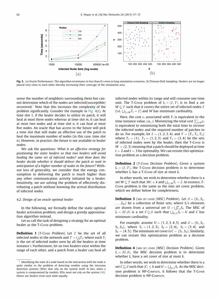
Fig. 5. (a) Oracle Performance: The algorithm terminates in less than 8 s even in long simulation scenarios. (b) Poisson Disk Sampling: Healers are no longerplaced very close to each other thereby increasing their coverage of the simulation area.
62 E. Hoque et al. / Ad Hoc Networks 24 (2015) 57–72
sense the number of neighbors surrounding them but can-not determine which of the nodes are infected/susceptible/recovered.1 Note that this increases the complexity of theproblem significantly. Consider the example in Fig. 4(c). Attime slot 1, if the healer decides to utilize its patch, it willheal at most three nodes whereas at time slot m, it can healat most two nodes and at time slot n, it can heal at mostfive nodes. An oracle that has access to the future will picka time slot that will make an effective use of the patch toheal the maximum number of nodes (in this case, time slotn). However, in practice, the future is not available to healernodes.
We ask the questions: What is an effective strategy forpositioning the static healers so that two healers will avoidhealing the same set of infected nodes? and How does thehealer decide whether it should deliver the patch or wait inanticipation of a higher number of nodes in the future? With-out loss of generality, we consider that the energy con-sumption in delivering the patch is much higher thanany other communication activity initiated by a healer.Intuitively, we are solving the problem of effectively dis-tributing a patch without knowing the arrival distributionof infected nodes.
4.2. Design of an oracle optimal healer
In the following, we formally define the static optimalhealer activation problem, and design a greedy approxima-tion algorithm instead.
Let us call the task of designing a strategy for an optimalhealer as the T-COVER problem.
Definition 1 (T-COVER Problem). Let I be the set of allinfected nodes in the network and T ¼
SiTi, where each Ti
is the set of infected nodes seen by all the healers at timeinstance i. Furthermore, let no two healers exist within therange of each other, and a patch from a healer can heal all
1 Identifying the state of a node based on the interaction with the node isquite similar to the problem of detecting rootkits using the intrusiondetection systems (IDSs) that rely on the system itself. In fact, when asystem is compromised by rootkits, IDSs must not rely on the system [40].Hence our healers treat each node equally.
infected nodes within its range and will consume one timeunit. The T-COVER problem of It ¼ ðI ; T Þ is to find a setW # T such that it covers the entire set of infected nodes I(i.e.
STi2W Ti ¼ I) and W has minimum cardinality.
Here, the cost ci associated with Ti is equivalent to thetime instance value, i.e., i. Minimizing the total cost
Pi2W ci
is equivalent to minimizing both the total time to recoverthe infected nodes and the required number of patches todo so. For example, let I ¼ f1;2;3;4g and T ¼ fT1; T2; T3gwhere T1 ¼ f1g; T2 ¼ f1;2;3g and T3 ¼ f3;4g be the setsof infected nodes seen by the healer, then the T-COVER isW ¼ f2;3gmeaning that a patch should be deployed at timet ¼ 2 and t ¼ 3 for optimality. We can restate this optimiza-tion problem as a decision problem.
Definition 2 (T-COVER Decision Problem). Given a systemIt ¼ ðI ; T Þ, the T-COVER decision problem is to determinewhether It has a T-COVER of size at most k.
In other words, we wish to determine whether there is aset W # T such that jWj 6 k and
STi2W Ti ¼ I . In essence, T-
COVER problem is the same as the min set cover problem,which we define below for completeness.
Definition 3 (MIN SET COVER (MSC) Problem). Let S ¼ fS1; S2;
. . . ; Smg be a collection of finite sets, where Si’s elementsare drawn from a universal set U ¼
Smi¼1Si. The MSC of
Is ¼ ðU;SÞ is a set C #S such thatS
Si2CSi ¼ U and C hasminimum cardinality.
For example, assume U ¼ f1;2;3;4;5g and S ¼ fS1; S2;
S3; S4g, where S1 ¼ f1;2;3g; S2 ¼ f2;4g, S3 ¼ f3;4g andS4 ¼ f4;5g. The minimum set cover is C ¼ fS1; S4g. Similarly,we can restate this optimization problem as a decisionproblem.
Definition 4 (MIN SET COVER (MSC) Decision Problem). GivenIs ¼ ðU;SÞ, the MSC decision problem is to determinewhether Is have a set cover of size at most k.
In other words, we wish to determine whether there is aset C #S such that jCj 6 k and U ¼
SSi2CSi. As the MSC deci-
sion problem is NP-COMPLETE, it follows that the T-COVER
decision problem is NP-COMPLETE.
E. Hoque et al. / Ad Hoc Networks 24 (2015) 57–72 63
Algorithm 1. Greedy Approximation (ORACLE).
Input Let I be the list of all infected nodes, Si be theset of infected nodes seen at each time i; wi be thelist of costs associated with each arrival at iInitially:
R is the set of elements that are not covered as yetC is the set of covered elementsw is the weight vectorR ¼ I and C ¼ /
repeatlet Si be the set that minimizes wi
jSi\RjC ¼ C [ fSigR ¼ R� Si
until R ¼ /return C
According to the above theorem, we can employ anyheuristic that solves the set cover problem to solve the T-COVER problem. Algorithm 1, based on the greedy set coveralgorithm [41], gives a greedy approximation for the T-COVER. The algorithm takes as input the arrival times ofthe infected nodes. Here, Si is the set of infected nodes seenat any one time instant and we equate the weight vector wi
to the time of arrival – cost of healing nodes at a later timeis higher because it introduces delay. The main loop iter-ates for OðnÞ time, where jI j ¼ n. The minimum W can befound in Oðlog mÞ time, using a priority heap, where thereare m sets in a set cover instance giving us a total time ofOðnlogðmÞÞ. Fig. 5(a) shows that even in the presence ofhundreds of thousands of node sets, we are able to com-pute the optimal solution in under 8 s.
4.3. Effective healer placement
Since the healers are static, the healer placement hasan impact on our defense protocols and thus their cover-age area depends on their placement strategy. Our simu-lations showed that a naive placement using uniformrandom distribution resulted in a scenario where manyhealers ended up covering the same region thereby leav-ing a lot of uncovered area. Another naive approach is thegrid placement of healers in which healers cover theentire arena and therefore each mobile node will alwaysbe in the range of at least one healer. This approachwould require N number of healers to cover the entirearena which could be a very large number depending onthe size of arena and the range of healers.2,3 Note thatthe infection containment problem becomes trivial in caseof grid placement. For instance, if healers were placed ingrids, the defense protocol would require all the healersto broadcast one patch each at the same time instance tand thus, the entire system would be recovered in one sec-ond at the cost of N patches. However, in realistic environ-ments, it is not practical to have so many static healers. We
2 For an arena of 500� 500 (m)2 and 20 m healer-range, N would be atleast 157, whereas we used N ¼ 20 healers for the same setup.
3 N would no longer be a fixed number.
focus instead of scenarios using a much smaller number ofstatic healers.
For our healer placement strategy, what we need is atype of a constraint that rejects certain configurations thatplace healers very close to each other. This problem can bedirectly reduced to a problem from the field of computervision which involves producing sampling patterns witha blue noise Fourier spectrum. Formally, the problem canbe defined as the limit of a uniform sampling process witha minimum-distance rejection criterion. Successive pointsare independently drawn from the uniform distribution½0;1�. If a point is at a distance of at least R from all pointsin the set of accepted points, it is added to that set. Other-wise, it is rejected. The choice of R controls the minimumallowable distance between points. This procedure calledPoisson Disk Sampling [42] has been actively studied andmany efficient algorithms exist. Due to space constraints,we do not discuss this algorithm further but refer thereader to the linear algorithm outlined by [42]. We adaptedthis algorithm by setting R ¼ 2r, where r is the range of oureach healer. Fig. 5(b) clearly highlights the merits of usingthis specific sampling process – healers are no longer closeto each other and hence cover more of the simulation area.
4.4. Family of randomized healers
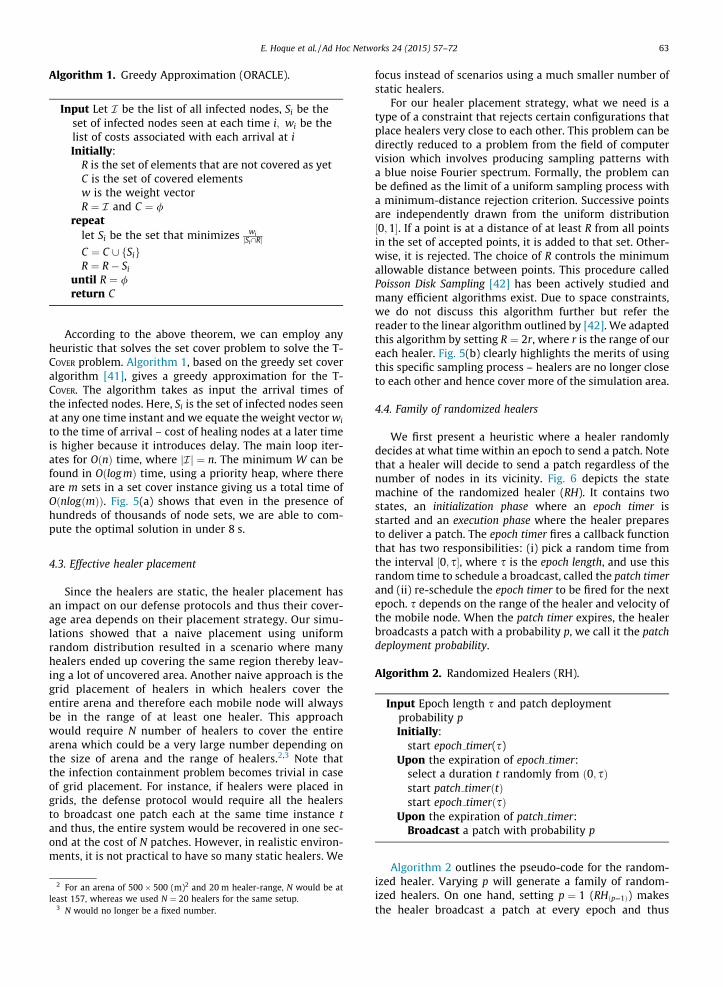
We first present a heuristic where a healer randomlydecides at what time within an epoch to send a patch. Notethat a healer will decide to send a patch regardless of thenumber of nodes in its vicinity. Fig. 6 depicts the statemachine of the randomized healer (RH). It contains twostates, an initialization phase where an epoch timer isstarted and an execution phase where the healer preparesto deliver a patch. The epoch timer fires a callback functionthat has two responsibilities: (i) pick a random time fromthe interval ½0; s�, where s is the epoch length, and use thisrandom time to schedule a broadcast, called the patch timerand (ii) re-schedule the epoch timer to be fired for the nextepoch. s depends on the range of the healer and velocity ofthe mobile node. When the patch timer expires, the healerbroadcasts a patch with a probability p, we call it the patchdeployment probability.
Algorithm 2. Randomized Healers (RH).
Input Epoch length s and patch deploymentprobability pInitially:
start epoch timer(s)Upon the expiration of epoch timer:
select a duration t randomly from ð0; sÞstart patch timerðtÞstart epoch timerðsÞ
Upon the expiration of patch timer:Broadcast a patch with probability p
Algorithm 2 outlines the pseudo-code for the random-ized healer. Varying p will generate a family of random-ized healers. On one hand, setting p ¼ 1 (RHðp¼1Þ) makesthe healer broadcast a patch at every epoch and thus
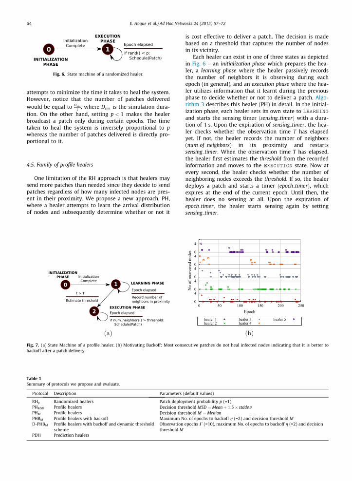
Fig. 6. State machine of a randomized healer.
64 E. Hoque et al. / Ad Hoc Networks 24 (2015) 57–72
attempts to minimize the time it takes to heal the system.However, notice that the number of patches deliveredwould be equal to Dsim
s , where Dsim is the simulation dura-tion. On the other hand, setting p < 1 makes the healerbroadcast a patch only during certain epochs. The timetaken to heal the system is inversely proportional to pwhereas the number of patches delivered is directly pro-portional to it.
4.5. Family of profile healers
One limitation of the RH approach is that healers maysend more patches than needed since they decide to sendpatches regardless of how many infected nodes are pres-ent in their proximity. We propose a new approach, PH,where a healer attempts to learn the arrival distributionof nodes and subsequently determine whether or not it
Table 1Summary of protocols we propose and evaluate.
Protocol Description Parameters (
RHp Randomized healers Patch deployPHMSD Profile healers Decision thrPHM Profile healers Decision thrPHBM Profile healers with backoff Maximum ND-PHBM Profile healers with backoff and dynamic threshold
schemeObservationthreshold M
PDH Prediction healers
Fig. 7. (a) State Machine of a profile healer. (b) Motivating Backoff: Most consbackoff after a patch delivery.
is cost effective to deliver a patch. The decision is madebased on a threshold that captures the number of nodesin its vicinity.
Each healer can exist in one of three states as depictedin Fig. 6 – an initialization phase which prepares the hea-ler, a learning phase where the healer passively recordsthe number of neighbors it is observing during eachepoch (in general), and an execution phase where the hea-ler utilizes information that it learnt during the previousphase to decide whether or not to deliver a patch. Algo-rithm 3 describes this healer (PH) in detail. In the initial-ization phase, each healer sets its own state to LEARNING
and starts the sensing timer ðsensing timerÞ with a dura-tion of 1 s. Upon the expiration of sensing timer, the hea-ler checks whether the observation time T has elapsedyet. If not, the healer records the number of neighbors(num of neighbors) in its proximity and restartssensing timer. When the observation time T has elapsed,the healer first estimates the threshold from the recordedinformation and moves to the EXECUTION state. Now atevery second, the healer checks whether the number ofneighboring nodes exceeds the threshold. If so, the healerdeploys a patch and starts a timer ðepoch timerÞ, whichexpires at the end of the current epoch. Until then, thehealer does no sensing at all. Upon the expiration ofepoch timer, the healer starts sensing again by settingsensing timer.
default values)
ment probability p (=1)eshold MSD ¼ Meanþ 1:5� stddeveshold M ¼ Mediano. of epochs to backoff g (=2) and decision threshold Mepochs C (=10), maximum No. of epochs to backoff g (=2) and decision
ecutive patches do not heal infected nodes indicating that it is better to
E. Hoque et al. / Ad Hoc Networks 24 (2015) 57–72 65
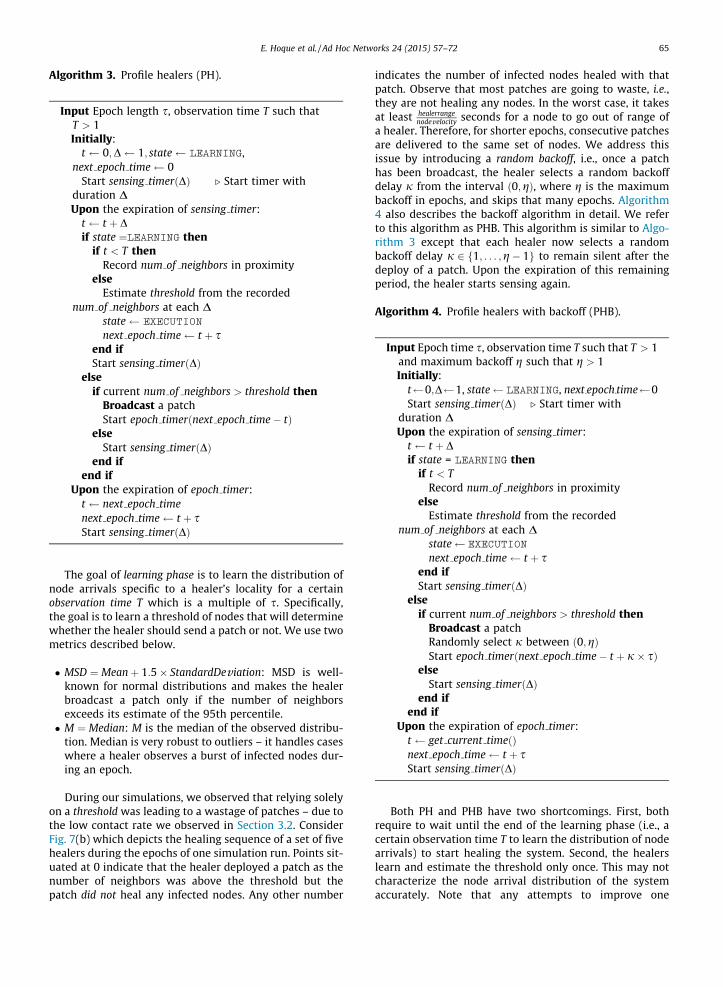
Algorithm 3. Profile healers (PH).
Input Epoch length s, observation time T such thatT > 1Initially:
t 0;D 1; state LEARNING,next epoch time 0
Start sensing timerðDÞ . Start timer withduration DUpon the expiration of sensing timer:
t t þ Dif state ¼LEARNING then
if t < T thenRecord num of neighbors in proximity
elseEstimate threshold from the recorded
num of neighbors at each Dstate EXECUTION
next epoch time t þ send ifStart sensing timerðDÞ
elseif current num of neighbors > threshold then
Broadcast a patchStart epoch timerðnext epoch time� tÞ
elseStart sensing timerðDÞ
end ifend if
Upon the expiration of epoch timer:t next epoch timenext epoch time t þ sStart sensing timerðDÞ
The goal of learning phase is to learn the distribution ofnode arrivals specific to a healer’s locality for a certainobservation time T which is a multiple of s. Specifically,the goal is to learn a threshold of nodes that will determinewhether the healer should send a patch or not. We use twometrics described below.
� MSD ¼ Meanþ 1:5� StandardDeviation: MSD is well-known for normal distributions and makes the healerbroadcast a patch only if the number of neighborsexceeds its estimate of the 95th percentile.� M ¼ Median: M is the median of the observed distribu-
tion. Median is very robust to outliers – it handles caseswhere a healer observes a burst of infected nodes dur-ing an epoch.
During our simulations, we observed that relying solelyon a threshold was leading to a wastage of patches – due tothe low contact rate we observed in Section 3.2. ConsiderFig. 7(b) which depicts the healing sequence of a set of fivehealers during the epochs of one simulation run. Points sit-uated at 0 indicate that the healer deployed a patch as thenumber of neighbors was above the threshold but thepatch did not heal any infected nodes. Any other number
indicates the number of infected nodes healed with thatpatch. Observe that most patches are going to waste, i.e.,they are not healing any nodes. In the worst case, it takesat least healerrange
nodevelocity seconds for a node to go out of range ofa healer. Therefore, for shorter epochs, consecutive patchesare delivered to the same set of nodes. We address thisissue by introducing a random backoff, i.e., once a patchhas been broadcast, the healer selects a random backoffdelay j from the interval ð0;gÞ, where g is the maximumbackoff in epochs, and skips that many epochs. Algorithm4 also describes the backoff algorithm in detail. We referto this algorithm as PHB. This algorithm is similar to Algo-rithm 3 except that each healer now selects a randombackoff delay j 2 f1; . . . ;g� 1g to remain silent after thedeploy of a patch. Upon the expiration of this remainingperiod, the healer starts sensing again.
Algorithm 4. Profile healers with backoff (PHB).
Input Epoch time s, observation time T such that T > 1and maximum backoff g such that g > 1Initially:
t 0;D 1, state LEARNING, next epoch time 0Start sensing timerðDÞ . Start timer with
duration DUpon the expiration of sensing timer:
t t þ Dif state = LEARNING then
if t < TRecord num of neighbors in proximity
elseEstimate threshold from the recorded
num of neighbors at each Dstate EXECUTION
next epoch time t þ send ifStart sensing timerðDÞ
elseif current num of neighbors > threshold then
Broadcast a patchRandomly select j between ð0;gÞStart epoch timerðnext epoch time� t þ j� sÞ
elseStart sensing timerðDÞ
end ifend if
Upon the expiration of epoch timer:t get current timeðÞnext epoch time t þ sStart sensing timerðDÞ
Both PH and PHB have two shortcomings. First, bothrequire to wait until the end of the learning phase (i.e., acertain observation time T to learn the distribution of nodearrivals) to start healing the system. Second, the healerslearn and estimate the threshold only once. This may notcharacterize the node arrival distribution of the systemaccurately. Note that any attempts to improve one
66 E. Hoque et al. / Ad Hoc Networks 24 (2015) 57–72
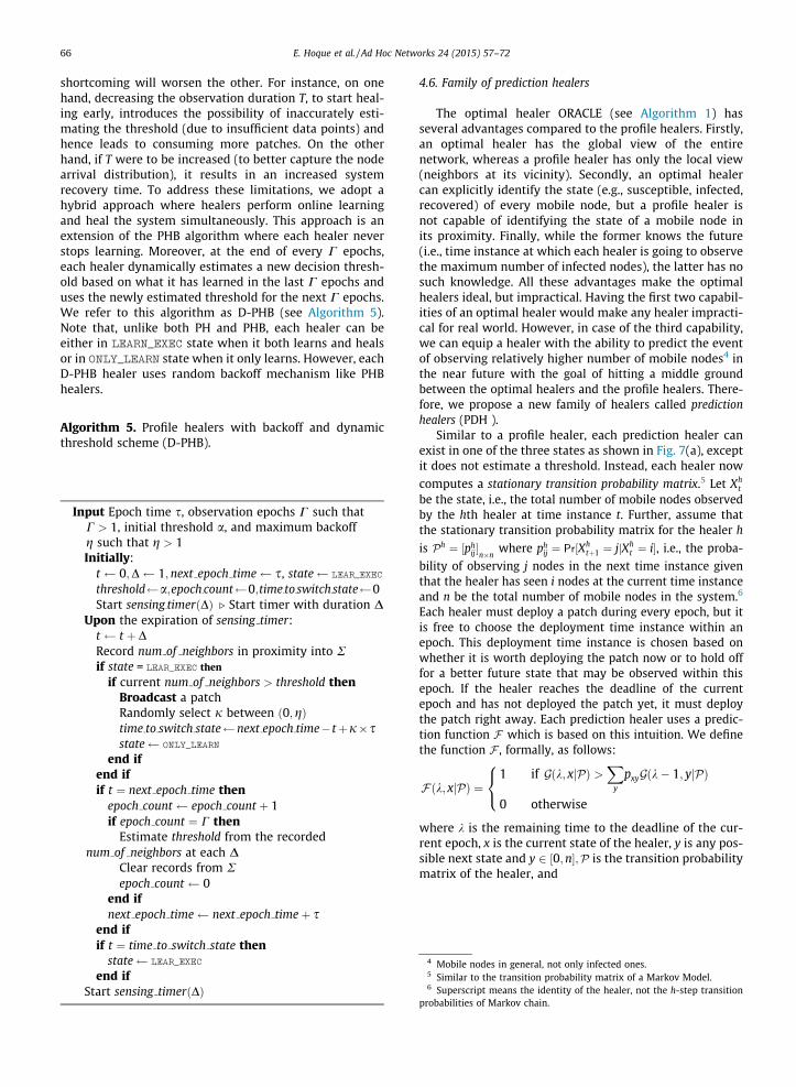
shortcoming will worsen the other. For instance, on onehand, decreasing the observation duration T, to start heal-ing early, introduces the possibility of inaccurately esti-mating the threshold (due to insufficient data points) andhence leads to consuming more patches. On the otherhand, if T were to be increased (to better capture the nodearrival distribution), it results in an increased systemrecovery time. To address these limitations, we adopt ahybrid approach where healers perform online learningand heal the system simultaneously. This approach is anextension of the PHB algorithm where each healer neverstops learning. Moreover, at the end of every C epochs,each healer dynamically estimates a new decision thresh-old based on what it has learned in the last C epochs anduses the newly estimated threshold for the next C epochs.We refer to this algorithm as D-PHB (see Algorithm 5).Note that, unlike both PH and PHB, each healer can beeither in LEARN_EXEC state when it both learns and healsor in ONLY_LEARN state when it only learns. However, eachD-PHB healer uses random backoff mechanism like PHBhealers.
Algorithm 5. Profile healers with backoff and dynamicthreshold scheme (D-PHB).
Input Epoch time s, observation epochs C such thatC > 1, initial threshold a, and maximum backoffg such that g > 1Initially:
t 0;D 1;next epoch time s, state LEAR_EXEC
threshold a;epoch count 0;time to switch state 0Start sensing timerðDÞ . Start timer with duration D
Upon the expiration of sensing timer:t t þ DRecord num of neighbors in proximity into Rif state = LEAR_EXEC then
if current num of neighbors > threshold thenBroadcast a patchRandomly select j between ð0;gÞtime to switch state next epoch time� tþj�sstate ONLY_LEARN
end ifend ifif t ¼ next epoch time then
epoch count epoch count þ 1if epoch count ¼ C then
Estimate threshold from the recordednum of neighbors at each D
Clear records from Repoch count 0
end ifnext epoch time next epoch timeþ s
end ifif t ¼ time to switch state then
state LEAR_EXEC
end ifStart sensing timerðDÞ
4.6. Family of prediction healers
The optimal healer ORACLE (see Algorithm 1) hasseveral advantages compared to the profile healers. Firstly,an optimal healer has the global view of the entirenetwork, whereas a profile healer has only the local view(neighbors at its vicinity). Secondly, an optimal healercan explicitly identify the state (e.g., susceptible, infected,recovered) of every mobile node, but a profile healer isnot capable of identifying the state of a mobile node inits proximity. Finally, while the former knows the future(i.e., time instance at which each healer is going to observethe maximum number of infected nodes), the latter has nosuch knowledge. All these advantages make the optimalhealers ideal, but impractical. Having the first two capabil-ities of an optimal healer would make any healer impracti-cal for real world. However, in case of the third capability,we can equip a healer with the ability to predict the eventof observing relatively higher number of mobile nodes4 inthe near future with the goal of hitting a middle groundbetween the optimal healers and the profile healers. There-fore, we propose a new family of healers called predictionhealers (PDH ).
Similar to a profile healer, each prediction healer canexist in one of the three states as shown in Fig. 7(a), exceptit does not estimate a threshold. Instead, each healer now
computes a stationary transition probability matrix.5 Let Xht
be the state, i.e., the total number of mobile nodes observedby the hth healer at time instance t. Further, assume thatthe stationary transition probability matrix for the healer h
is Ph ¼ ½phij�n�n
where phij ¼ Pr½Xh
tþ1 ¼ jjXht ¼ i�, i.e., the proba-
bility of observing j nodes in the next time instance giventhat the healer has seen i nodes at the current time instanceand n be the total number of mobile nodes in the system.6
Each healer must deploy a patch during every epoch, but itis free to choose the deployment time instance within anepoch. This deployment time instance is chosen based onwhether it is worth deploying the patch now or to hold offfor a better future state that may be observed within thisepoch. If the healer reaches the deadline of the currentepoch and has not deployed the patch yet, it must deploythe patch right away. Each prediction healer uses a predic-tion function F which is based on this intuition. We definethe function F , formally, as follows:
Fðk; xjPÞ ¼1 if Gðk; xjPÞ >
Xy
pxyGðk� 1; yjPÞ
0 otherwise
8<:
where k is the remaining time to the deadline of the cur-rent epoch, x is the current state of the healer, y is any pos-sible next state and y 2 ½0;n�;P is the transition probabilitymatrix of the healer, and
4 Mobile nodes in general, not only infected ones.5 Similar to the transition probability matrix of a Markov Model.6 Superscript means the identity of the healer, not the h-step transition
probabilities of Markov chain.
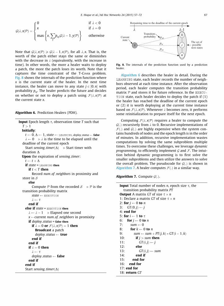
Fig. 8. The internals of the prediction function used by a predictionhealer.
E. Hoque et al. / Ad Hoc Networks 24 (2015) 57–72 67
Gðk; xjPÞ ¼
0 if k < 0x if k ¼ 0
max x;X
y
pxyGðk� 1; yjPÞ( )
otherwise
8>>><>>>:
Note that Gðk; xjPÞP Gðk� 1; xjPÞ, for all k; x. That is, theworth of the patch either stays the same or diminisheswith the decrease in k (equivalently, with the increase intime). In other words, the more a healer waits to deploya patch, the more the patch loses its worth. Note that itcaptures the time constraint of the T-COVER problem.Fig. 8 shows the internals of the prediction function wherex is the current state of the healer. In the next timeinstance, the healer can move to any state j 2 ½0;n� withprobability pxj. The healer predicts the future and decideson whether or not to deploy a patch using Fðk; xjPÞ atthe current state x.
Algorithm 6. Prediction Healers (PDH).
Input Epoch length s, observation time T such thatT > 1Initially:
t 0;D 1, state LEARNING, deploy status false
k 0 . k is the time to be elapsed until thedeadline of the current epoch
Start sensing timerðDÞ . Start timer withduration DUpon the expiration of sensing timer:
t t þ Dif state = LEARNING then
if t < T thenRecord num of neighbors in proximity and
store in Selse
Compute P from the recorded S . P is thetransition probability matrix
state EXECUTION
k send if
else if state = EXECUTION then
k k� 1 . Elapsed one secondx current num of neighbors in promixityif deploy status = false then
if k ¼ 0 or Fðk; xjPÞ ¼ 1 thenBroadcast a patchdeploy status true
end ifend ifif k ¼ 0 then
k sdeploy status false
end ifend ifStart sensing timerðDÞ
Algorithm 6 describes the healer in detail. During theLEARNING state, each healer records the number of neigh-bors observed at each time instance. After the observationperiod, each healer computes the transition probabilitymatrix P and stores it for future reference. In the EXECU-
TION state, each healer decides to deploy the patch if (1)the healer has reached the deadline of the current epochor (2) it is worth deploying at the current time instancebased on Fðk; xjPÞ. Whenever k becomes zero, it performssome reinitialization to prepare itself for the next epoch.
Computing Fðk; xjPÞ requires a healer to compute theGð:Þ recursively from k to 0. Recursive implementations ofFð:Þ and Gð:Þ are highly expensive when the system con-tains hundreds of nodes and the epoch length is in the orderof minutes. In addition, recursive implementation wastescomputations by solving the same subproblem multipletimes. To overcome these challenges, we leverage dynamicprogramming, to efficiently implement G and F . The intui-tion behind dynamic programming is to first solve thesmaller subproblems and then utilize the answers to solvethe overall problem. The pseudocode for Gð:Þ is shown inAlgorithm 7. A healer computes Fð:Þ in a similar way.
Algorithm 7. Compute Gð:Þ.
Input Total number of nodes n, epoch size s, thetransition probability matrix PT
Output A matrix GT of size s� n1: Declare a matrix GT of size s� n2: for j 0 to n3: GTð0; jÞ j4: end for5: for i 1 to s6: for j 0 to n7: sum 08: for k 0 to n9: sum sumþ PTðj; kÞ � GTði� 1; kÞ10: if j > sum then11: GTði; jÞ j12: else13: GTði; jÞ sum14: end if15: end for16: end for17: end for18: return GT
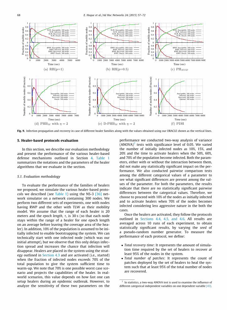
Fig. 9. Infection propagation and recovery in case of different healer families along with the values obtained using our ORACLE shown as the vertical lines.
7 In statistics, a two-way ANOVA test is used to examine the influence ofdifferent categorical independent variables on one dependent variable [43].
68 E. Hoque et al. / Ad Hoc Networks 24 (2015) 57–72
5. Healer-based protocols evaluation
In this section, we describe our evaluation methodologyand present the performance of the various healer-baseddefense mechanisms outlined in Section 4. Table 1summarizes the notations and the parameters of the healeralgorithms that we evaluate in the section.
5.1. Evaluation methodology
To evaluate the performance of the families of healerswe proposed, we simulate the various healer-based proto-cols we described (see Table 1) using the NS-3 [36] net-work simulator on a network containing 300 nodes. Weperform two different sets of experiments, one with nodeshaving RWP and the other with TLW as their mobilitymodel. We assume that the range of each healer is 20meters and the epoch length, s, is 30 s (so that each nodestays within the range of a healer for one epoch lengthon an average before leaving the coverage area of the hea-ler). In addition, 10% of the population is assumed to be ini-tially infected to enable bootstrapping the system. We cantechnically start with one infected node (which was ourinitial attempt), but we observe that this only delays infec-tion spread and increases the chance that infection willdisappear. Healers are placed in the system using the strat-egy outlined in Section 4.3 and are activated (i.e., started)when the fraction of infected nodes exceeds 70% of thetotal population to give the system sufficient time towarm-up. We note that 70% is one possible worst case sce-nario and projects the capabilities of the healer. In real-world scenarios, this value depends on how fast one cansetup healers during an epidemic outbreak. However, toanalyze the sensitivity of these two parameters on the
performance we conducted two-way analysis of variance(ANOVA)7 tests with significance level of 0.05. We variedthe number of initially infected nodes as 10%, 15%, and20% and the time to activate healers when the 50%, 60%,and 70% of the population become infected. Both the param-eters, either with or without the interaction between them,did not make any statistically significant impact on the per-formance. We also conducted pairwise comparison testsamong the different categorical values of a parameter tosee what significant differences are present among the val-ues of the parameter. For both the parameters, the resultsindicate that there are no statistically significant pairwisedifferences between the categorical values. Therefore, wechoose to proceed with 10% of the nodes as initially infectedand to activate healers when 70% of the nodes becomesinfected considering less aggressive nature in the both thecases.
Once the healers are activated, they follow the protocolsoutlined in Sections 4.4, 4.5, and 4.6. All results areaveraged across 10 runs of each experiment, to obtainstatistically significant results, by varying the seed ofa pseudo-random number generator. To measure theperformance of each protocol, we define:
� Total recovery time: It represents the amount of simula-tion time required by the set of healers to recover atleast 95% of the nodes in the system.� Total number of patches: It represents the count of
patches deployed by the set of healers to heal the sys-tem such that at least 95% of the total number of nodesare recovered.
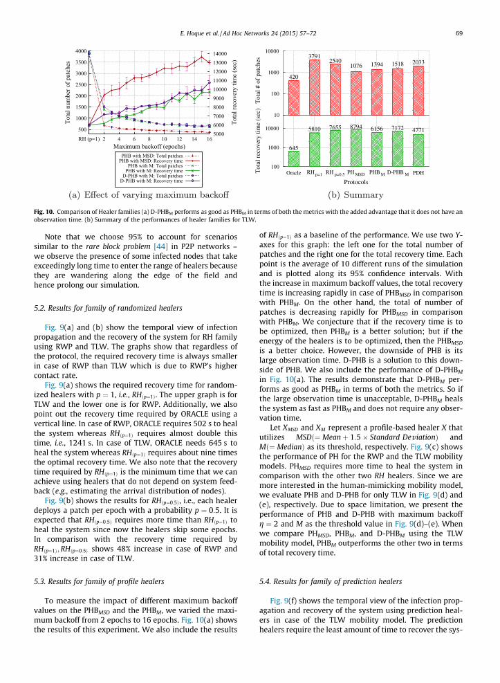
Fig. 10. Comparison of Healer families (a) D-PHBM performs as good as PHBM in terms of both the metrics with the added advantage that it does not have anobservation time. (b) Summary of the performances of healer families for TLW.
E. Hoque et al. / Ad Hoc Networks 24 (2015) 57–72 69
Note that we choose 95% to account for scenariossimilar to the rare block problem [44] in P2P networks –we observe the presence of some infected nodes that takeexceedingly long time to enter the range of healers becausethey are wandering along the edge of the field andhence prolong our simulation.
5.2. Results for family of randomized healers
Fig. 9(a) and (b) show the temporal view of infectionpropagation and the recovery of the system for RH familyusing RWP and TLW. The graphs show that regardless ofthe protocol, the required recovery time is always smallerin case of RWP than TLW which is due to RWP’s highercontact rate.
Fig. 9(a) shows the required recovery time for random-ized healers with p ¼ 1, i.e., RHðp¼1Þ. The upper graph is forTLW and the lower one is for RWP. Additionally, we alsopoint out the recovery time required by ORACLE using avertical line. In case of RWP, ORACLE requires 502 s to healthe system whereas RHðp¼1Þ requires almost double thistime, i.e., 1241 s. In case of TLW, ORACLE needs 645 s toheal the system whereas RHðp¼1Þ requires about nine timesthe optimal recovery time. We also note that the recoverytime required by RHðp¼1Þ is the minimum time that we canachieve using healers that do not depend on system feed-back (e.g., estimating the arrival distribution of nodes).
Fig. 9(b) shows the results for RHðp¼0:5Þ, i.e., each healerdeploys a patch per epoch with a probability p ¼ 0:5. It isexpected that RHðp¼0:5Þ requires more time than RHðp¼1Þ toheal the system since now the healers skip some epochs.In comparison with the recovery time required byRHðp¼1Þ;RHðp¼0:5Þ shows 48% increase in case of RWP and31% increase in case of TLW.
5.3. Results for family of profile healers
To measure the impact of different maximum backoffvalues on the PHBMSD and the PHBM, we varied the maxi-mum backoff from 2 epochs to 16 epochs. Fig. 10(a) showsthe results of this experiment. We also include the results
of RHðp¼1Þ as a baseline of the performance. We use two Y-axes for this graph: the left one for the total number ofpatches and the right one for the total recovery time. Eachpoint is the average of 10 different runs of the simulationand is plotted along its 95% confidence intervals. Withthe increase in maximum backoff values, the total recoverytime is increasing rapidly in case of PHBMSD in comparisonwith PHBM. On the other hand, the total of number ofpatches is decreasing rapidly for PHBMSD in comparisonwith PHBM. We conjecture that if the recovery time is tobe optimized, then PHBM is a better solution; but if theenergy of the healers is to be optimized, then the PHBMSD
is a better choice. However, the downside of PHB is itslarge observation time. D-PHB is a solution to this down-side of PHB. We also include the performance of D-PHBM
in Fig. 10(a). The results demonstrate that D-PHBM per-forms as good as PHBM in terms of both the metrics. So ifthe large observation time is unacceptable, D-PHBM healsthe system as fast as PHBM and does not require any obser-vation time.
Let XMSD and XM represent a profile-based healer X thatutilizes MSDð¼ Meanþ 1:5� Standard DeviationÞ andMð¼ MedianÞ as its threshold, respectively. Fig. 9(c) showsthe performance of PH for the RWP and the TLW mobilitymodels. PHMSD requires more time to heal the system incomparison with the other two RH healers. Since we aremore interested in the human-mimicking mobility model,we evaluate PHB and D-PHB for only TLW in Fig. 9(d) and(e), respectively. Due to space limitation, we present theperformance of PHB and D-PHB with maximum backoffg ¼ 2 and M as the threshold value in Fig. 9(d)–(e). Whenwe compare PHMSD, PHBM, and D-PHBM using the TLWmobility model, PHBM outperforms the other two in termsof total recovery time.
5.4. Results for family of prediction healers
Fig. 9(f) shows the temporal view of the infection prop-agation and recovery of the system using prediction heal-ers in case of the TLW mobility model. The predictionhealers require the least amount of time to recover the sys-
70 E. Hoque et al. / Ad Hoc Networks 24 (2015) 57–72
tem when compared to the RH and PH families. This is dueto the prediction capability of the healers that allow themto deploy patches efficiently. The recovery time requiredby the prediction healers is 18% less and 22.5% less thanthe best random healers RHðp¼1Þ and the best profile healersPHBM, respectively.
Summary: Fig. 10(b) summarizes the results consistingof both the metrics obtained by each of the healers for theTLW mobility model. In terms of the number of patches,PHMSD requires the least number of patches but at the costof a larger recovery time. The prediction healers PDH out-performs the others in terms of the total recovery time.However, it requires 89% more patches than PHMSD. Nextcomes the RHðp¼1Þ that requires 21% more recovery timethan PDH. However, in order to achieve this recovery,RHðp¼1Þ has to deploy the maximum amount of patches.In fact, PHBM performs the best since it requires only 29%more recovery time in comparison to PDH and only 30%more patches than that of PHMSD.
Our results show that each of the schemes has advanta-ges and disadvantages. First, randomized healers offer theimmediate advantage that they do not rely on system feed-back nor do they have to learn the system before startingto recover the system. Second, prediction healers wouldbe beneficial in a time-constrained system as these healersare fastest at recovering an infected system by utilizingprediction capability. However, they result in using 1.8�patches than the profile healers (with MSD threshold).Finally, profile healers with backoff offer intelligent deci-sion making thereby saving energy in the form of utilizingless number of patches and would benefit the most in anenergy-constrained environment. However, they result intaking 1.8� time to recover in comparison to PDH healers.On the other hand, when compared with the ORACLE, weobserve that PDH, RH, and PHBM healers take 7.4�, 9�,and 9.5� recovery time, respectively. Furthermore, torecover the system PHMSD healers require 2.5� patchesthan the ORACLE.
6. Related work
We divide this section into two parts. In the first part,we discuss related work in the area of mathematical mod-eling and analysis of worms and viral epidemics. We thenmove on to discussing the existing works on controllingthe worm propagation.
Epidemic models. Wired networks have been the focusof most literature on worm propagation. A comprehensiveoverview of major malware outbreaks in networks with adiscussion of their trends is given in [45]. There are twopopular models that are generally used to describe wormpropagation: deterministic [5,7,46–50,6] and stochastic[51,52] epidemiological models. Staniford et al. [48] usethe SIR epidemiological model to capture the effects ofhuman countermeasures and the congestion due to theworm spread. Shen et al. [53] provide a discrete-timeworm model that considers patching, cleaning and certainlocal scanning techniques. All these approaches abstractnetwork topology and change in the size of vulnerablepopulation as the worm spreads. Theodorakopoulos et al.
[54] take deterministic modeling one step further andcombine it with a game theoretic process that involveslearning. A probabilistic queueing framework has beenproposed in [55] to model the spread of mobile virusesusing short range wireless interfaces (e.g., Bluetooth) ofmobile devices. While similar in spirit, our work focuseson modeling infection dynamics in MANETs as a functionof the mobility models.
Peng et al. [56] propose a two-dimensional cellularautomata to characterize the propagation dynamics ofworms in smartphones. Their scheme integrates an infec-tion factor evaluate the spread degree of infected nodes,and a resistance factor to evaluate the degree that suscep-tible nodes resist. Wang et al. [57] deploy agents in theform of hidden contacts on the device to capture messagessent from malicious applications. The authors combinethese captured messages in conjunction with a latent spacemodel to estimate the current dynamics of the system anduse this to predict the future state of malware propagationwithin the mobility network. Our work is complementaryto these efforts in that our decentralized algorithms canutilize their models during the learning phase. Szongottet al. [58] present a prototype of a replicating mobile mal-ware that spreads from device to device in downtown Chi-cago. Using simulations, they show that smartphonescreate a viable substrate for epidemic mobile malware.Our work differs from them in two key aspects. First, unlikethem, we use a more realistic truncated levy walk mobilitymodel. Second, they only study infection propagationwhereas we propose several algorithms for recovery.
Worm containment. There have been some works incontrolling the spread of worms inside a wireless network[59,60,8,61,20,21]. Williamson et al. [59] present a tech-nique to limit the rate of connections to ‘‘new’’ machines.This is effective at both slowing and halting virus propaga-tion without affecting normal traffic. Their work is basedon heuristics and simulations which consider a staticchoice of reduced communication rate. Wong et al. [60]present a technique that relies on limiting the contact rateof worm traffic. Specifically, they investigate rate control atindividual end hosts and at the edge and backbone routers,for both random propagation and local-preferentialworms. They show that both host and edge-router basedrate control result in a slowdown that is linear to the num-ber of hosts implementing the rate limiting filter.
More recently, Barbera et al. [62] consider the problemof computing an efficient patching strategy to stop wormspreading between smartphones. They consider caseswhere the worm spreads between the devices and wherethe worm attacks the cloud before moving to the device.Tang et al. [63] propose distributing patches to certainkey nodes so they can opportunistically disseminate themto the rest of the network. In their work, they present apredictive mobile malware containment system wheredevices collect co-location data in a decentralized mannerand report to a central server which processes and targetsdelivery of hot fixes to a small subset of k devices at run-time. In contrast, our work does not assume a central ser-ver and all our algorithms are fully decentralized.
Cole et al. [61] present both analytic and simulationanalysis of worm propagation focusing specifically on the
E. Hoque et al. / Ad Hoc Networks 24 (2015) 57–72 71
features of a tactical, battlefield MANETs which are uniqueto a defense environment. Their goal was to develop anaccurate set of performance requirements on potentialmitigation techniques of worm propagation for such MAN-ETs. Zou et al. [64] compare email worm propagation onthree topologies: power law, small world, and randomgraph topologies; and then study how the topology affectsimmunization defense on email worms. Their email wormmodel includes the effect of human interactions. Yang et al.[65] utilize a software diversity approach to deal with thespread of worm in wireless sensor networks. Zhu et al. [66]take into account the social relationship of mobile users tocontain MMS worms within a limited range in cellular net-works. Unlike them, we introduce a suite of defense proto-cols used by a set of static healers to thwart the epidemicspread inside MANETs.
7. Conclusion
Mobile malware have become an emerging problemthat threatens smartphones which are growing signifi-cantly in recent days. In this paper, we considered realisticmobility patterns to model proximity dependent malwareand compared them against de facto models like randomwaypoint mobility model. We presented several defensemechanisms that allow tuning of parameters to controltwo dimensions of optimization – either time to recoveryor energy utilized. The extensive evaluation of all ourdefense mechanisms shows that prediction healers wouldbe more effective in a time constrained environmentwhereas profile healers would benefit the most in anenergy constrained environment.
References
[1] R. Potharaju, E. Hoque, C. Nita-Rotaru, S. Sarkar, S. Venkatesh, Closingthe pandora’s box: defenses for thwarting epidemic outbreaks inmobile adhoc networks, in: Proc. of IEEE MASS, 2012, pp. 200–208.
[2] McAfee Threats Report: 3rd Quarter 2011. <http://goo.gl/jIQPJ>.[3] Juniper Mobile Threats Report 2010-11. <http://goo.gl/v3yFg>.[4] D. Moore, V. Paxson, S. Savage, C. Shannon, S. Staniford, N. Weaver,
Inside the slammer worm, IEEE Secur. Privacy 1 (4) (2003) 33–39.
[5] C.C. Zou, W. Gong, D. Towsley, Code red worm propagation modelingand analysis, in: Proc. of CCS, ACM, 2002, pp. 138–147.
[6] A. Wagner, T. Dübendorfer, B. Plattner, R. Hiestand, Experiences withworm propagation simulations, in: Proc. of WORM, ACM, 2003, pp.34–41.
[7] J.O. Kephart, S.R. White, Directed-graph epidemiological models ofcomputer viruses, in: Proc. of Sym. on Research in Sec. and Priv, IEEECompSoc, 1991, pp. 343–359.
[8] S.H. Sellke, N.B. Shroff, S. Bagchi, Modeling and automatedcontainment of worms, IEEE TDSC 5 (2) (2008) 71–86.
[9] Single NFC bonk subjugated Samsung Galaxy SIII and slurped it out,2012. <http://www.theregister.co.uk/2012/09/21/android_nfc/>.
[10] C. Miller, Exploring the NFC attack surface, in: Blackhat, 2012.[11] McAfee warns of NFC malware risk, 2013. <http://www.itpro.co.uk/
malware/19275/mcafee-warns-nfc-malware-risk>.[12] Wall Of Sheep Hacker Group Exposes NFC’s Risks At Def Con 2013,
2013. <http://www.forbes.com/sites/michaelvenables/2013/08/08/wall-of-sheep-near-field-communication-hack-at-def-con/2/>.
[13] A. Khelil, C. Becker, J. Tian, K. Rothermel, An epidemic model forinformation diffusion in manets, in: Proc. of MSWiM, ACM, 2002, pp.54–60.
[14] A. Bose, X. Hu, K.G. Shin, T. Park, Behavioral detection of malware onmobile handsets, in: Proc. of ACM Mobisys, ACM, 2008, pp. 225–238.
[15] C. Fleizach, M. Liljenstam, P. Johansson, G.M. Voelker, A. Mehes, Canyou infect me now? Malware propagation in mobile phonenetworks, in: Proc. of ACM WORM, ACM, 2007, pp. 61–68.
[16] A. Bose, K.G. Shin, On mobile viruses exploiting messaging andbluetooth services, in: Proc. of SecureComm, IEEE, 2006, pp. 1–10.
[17] G. Zyba, G.M. Voelker, M. Liljenstam, A. Méhes, P. Johansson,Defending mobile phones from proximity malware, in: Proc. ofINFOCOM, IEEE, 2009, pp. 1503–1511.
[18] R. Potharaju, C. Nita-Rotaru, Pandora: a platform for wormsimulations in mobile ad-hoc networks, ACM SIGMOBILE MobileComput. Commun. Rev. 14 (4) (2011) 16–18.
[19] I. Rhee, M. Shin, S. Hong, K. Lee, S.J. Kim, S. Chong, On the levy-walknature of human mobility, IEEE/ACM Trans. Netw. 19 (3) (2011)630–643.
[20] M. Khouzani, E. Altman, S. Sarkar, Optimal quarantining of wirelessmalware through reception gain control, IEEE Trans. Autom. Control57 (1) (2012) 49–61.
[21] M. Khouzani, S. Sarkar, E. Altman, Optimal dissemination of securitypatches in mobile wireless networks, IEEE Trans. Inf. Theory 58 (7)(2012) 4714–4732.
[22] J. Broch, D.A. Maltz, D.B. Johnson, Y.-C. Hu, J. Jetcheva, A performancecomparison of multi-hop wireless ad hoc network routing protocols,in: Proc. of MobiCom, ACM, 1998, pp. 85–97.
[23] C.-C. Chiang, M. Gerla, On-demand multicast in mobile wirelessnetworks, in: Proc. of ICNP, IEEE, 1998, pp. 262–270.
[24] J.J. Garcia-Luna-Aceves, M. Spohn, Source-tree routing in wirelessnetworks, in: Proc. of ICNP, IEEE, 1999, pp. 273–282.
[25] D.B. Johnson, D.A. Maltz, Dynamic source routing in ad hoc wirelessnetworks, Kluwer Int. Ser. Eng. Comput. Sci. (1996) 153–179.
[26] T. Camp, J. Boleng, V. Davies, A survey of mobility models for ad hocnetwork research, W. Comm. Mobile Comp. 2 (5) (2002) 483–502.
[27] M.C. Gonzalez, C.A. Hidalgo, A.-L. Barabasi, Understanding individualhuman mobility patterns, Nature 453 (7196) (2008) 779–782.
[28] J. Boleng, Normalizing mobility characteristics and enablingadaptive protocols for ad hoc networks, in: Proc. of LANMAN,2001, pp. 9–12.
[29] K. Lee, S. Hong, S.J. Kim, I. Rhee, S. Chong, Slaw: a new mobility modelfor human walks, in: Proc. of INFOCOM, IEEE, 2009, pp. 855–863.
[30] C. Boldrini, A. Passarella, Hcmm: modelling spatial and temporalproperties of human mobility driven by users social relationships,Comput. Commun. 33 (9) (2010) 1056–1074.
[31] S. Isaacman, R. Becker, R. Cáceres, M. Martonosi, J. Rowland, A.Varshavsky, W. Willinger, Human mobility modeling atmetropolitan scales, in: Proc. of MobiSys, ACM, 2012, pp. 239–252.
[32] V. Capasso, G. Serio, A generalization of the Kermack–McKendrickdeterministic epidemic model, Math. Biosci. 42 (1) (1978) 43–61.
[33] C.-Y. Huang, C.-T. Sun, H.-C. Lin, Influence of local information onsocial simulations in small-world network models, J. Artif. Soc. Soc.Simul. 8 (4) (2005) 8.
[34] R. Potharaju, Infection quarantining for wireless networks usingpower control, in: DSN Student Forum, 2010.
[35] C. de Waal, M. Gerharz, Bonnmotion: A mobility scenario generationand analysis tool, Communication Systems group, Institute ofComputer Science IV, University of Bonn, Germany, 2003.
[36] The Network Simulator – NS-3. <http://www.nsnam.org>.[37] C. Bettstetter, C. Wagner, et al., The spatial node distribution of the
random waypoint mobility model, in: German Workshop on MobileAd Hoc Networks (WMAN), 2002, pp. 41–58.
[38] G. Resta, P. Santi, An analysis of the node spatial distribution of therandom waypoint mobility model for ad hoc networks, in: Proc. ofPOMC, ACM, 2002, pp. 44–50.
[39] E. Hyytiä, J. Virtamo, Random waypoint mobility model in cellularnetworks, Wirel. Netw. 13 (2) (2007) 177–188.
[40] J. Levine, J.B. Grizzard, H.L. Owen, Detecting and categorizing kernel-levelrootkits to aid future detection, IEEE Secur. Privacy 4 (1) (2006) 24–32.
[41] V.V. Vazirani, Approximation Algorithms, Springer-Verlag, NewYork, Inc., 2001.
[42] R. Bridson, Fast poisson disk sampling in arbitrary dimensions, in:ACM SIGGRAPH, vol. 2007, 2007.
[43] Two-way analysis of variance. <http://en.wikipedia.org/wiki/Two-way_analysis_of_variance>.
[44] C. Gkantsidis, P.R. Rodriguez, Network coding for large scale contentdistribution, Proc. of IEEE INFOCOM, Vol. 4, IEEE, 2005, pp. 2235–2245.
[45] D. Kienzle, M. Elder, Recent worms: a survey and trends, in: Proc. ofWORM, ACM, 2003, pp. 1–10.
[46] J. Kephart, S. White, D. Chess, Computers and epidemiology, IEEESpectrum 30 (5) (1993) 20–26.
[47] J. Kephart, S. White, Measuring and modeling computer virusprevalence, in: Proc. of IEEE S&P, IEEE Computer Society, 1993, p. 2.
[48] S. Staniford, V. Paxson, N. Weaver, How to own the internet in yourspare time, in: Proc. of USENIX Security, vol. 8, 2002, pp. 149–167.
72 E. Hoque et al. / Ad Hoc Networks 24 (2015) 57–72
[49] G. Serazzi, S. Zanero, Computer virus propagation models, Perform.Tools Appl. Netw. Syst. (2004) 26–50.
[50] G. Kesidis, I. Hamadeh, S. Jiwasurat, Coupled Kermack–McKendrickmodels for randomly scanning and bandwidth-saturating internetworms, Qual. Ser. Multiserv. IP Netw. (2005) 101–109.
[51] R. Anderson, R. May, Infectious Diseases of Humans: Dynamics andControl, Oxford University Press, 1992.
[52] H. Andersson, T. Britton, Stochastic Epidemic Models and TheirStatistical Analysis, Springer Verlag, 2000.
[53] Z. Chen, L. Gao, K. Kwiat, Modeling the spread of active worms, Proc.of INFOCOM, vol. 3, IEEE, 2003, pp. 1890–1900.
[54] G. Theodorakopoulos, J. Baras, J. Le Boudec, Dynamic networksecurity deployment under partial information, in: Proc. ofAllerton, 2008, pp. 261–267.
[55] J.W. Mickens, B.D. Noble, Modeling epidemic spreading inmobile environments, in: Proc. of ACM WiSe, ACM, 2005, pp. 77–86.
[56] S. Peng, G. Wang, S. Yu, Modeling the dynamics of worm propagationusing two-dimensional cellular automata in smartphones, J.Comput. Syst. Sci. 79 (5) (2013) 586–595.
[57] W. Wang, I. Murynets, J. Bickford, C.V. Wart, G. Xu, What you seepredicts what you get lightweight agent-based malware detection,Secur. Commun. Netw. 6 (1) (2013) 33–48.
[58] C. Szongott, B. Henne, M. Smith, Evaluating the threat of epidemicmobile malware, in: 20012 IEEE 8th International Conference onWireless and Mobile Computing, Networking and Communications(WiMob), IEEE, 2012, pp. 443–450.
[59] M.M. Williamson, Throttling viruses: restricting propagation todefeat malicious mobile code, in: Proc. of ACSAC, IEEE, 2002, pp.61–68.
[60] C. Wong, C. Wang, D. Song, S. Bielski, G.R. Ganger,Dynamic quarantine of internet worms, in: Proc. of DSN, IEEE, 2004,pp. 73–82.
[61] R.G. Cole, Initial Studies on Worm Propagation in MANETsfor Future Army Combat Systems, Tech. rep., DTIC Document,2004.
[62] M.V. Barbera, S. Kosta, J. Stefa, P. Hui, A. Mei, Cloudshield: efficientanti-malware smartphone patching with a P2P network on thecloud, in: 2012 IEEE 12th International Conference on Peer-to-PeerComputing (P2P), IEEE, 2012, pp. 50–56.
[63] J. Tang, H. Kim, C. Mascolo, M. Musolesi, Stop: socio-temporalopportunistic patching of short range mobile malware, in:2012 IEEE International Symposium on a World of Wireless,Mobile and Multimedia Networks (WoWMoM), IEEE, 2012, pp. 1–9.
[64] C.C. Zou, D. Towsley, W. Gong, Email worm modeling and defense,in: Proc. of ICCCN, IEEE, 2004, pp. 409–414.
[65] Y. Yang, S. Zhu, G. Cao, Improving sensor network immunity underworm attacks: a software diversity approach, in: Proc. of ACMMobiHoc, ACM, 2008, pp. 149–158.
[66] Z. Zhu, G. Cao, S. Zhu, S. Ranjan, A. Nucci, A social network basedpatching scheme for worm containment in cellular networks, in:Handbook of Optimization in Complex Networks, Springer, 2012, pp.505–533.
Endadul Hoque is a PhD student in theComputer Science Department at PurdueUniversity under the supervision of ProfessorCristina Nita-Rotaru. He obtained his MS inComputer Science from Marquette University,WI, in 2010 and BS in Computer Science andEngineering from Bangladesh University ofEngineering & Technology (BUET), Bangla-desh, in 2008. He is a member of theDependable and Secure Distributed SystemsLaboratory (DS2). His research interestsinclude security in wireless networks and
distributed systems. He is a member of the ACM and IEEE ComputerSociety.
Rahul Potharaju is an Applied Scientist in theCloud and Information Services Lab at Micro-soft. Before that, he obtained his PhD degreein Computer Science from Purdue Universityand Master’s degree in Computer Sciencefrom Northwestern University. Rahul is pas-sionate about transforming big data intoactionable insights and building large-scaledata-intensive systems, with a particularinterest in analytics-as-a-service clouds andautomated problem inference systems. He is arecipient of the Motorola Engineering Excel-
lence award in 2009 and the Purdue Diamond Award in 2014. Hisresearch has been adopted by several business groups inside Microsoftand has won the Microsoft Trustworthy Reliability Computing Award in
2013.Cristina Nita-Rotaru is an Associate Professorin the department of Computer Science atPurdue University. She leads the Dependableand Secure Distributed Systems Laboratory.She received BS and MS degrees from Poli-technica University of Bucharest, Romania, in1995 and 1996, and a PhD degree in ComputerScience from The Johns Hopkins University in2003. She served on the technical programcommittee of over 40 conference in net-working, distributed systems, and security.She received the NSF CAREER award. Her
research interests include security and fault-tolerance for distributedsystems, and networks. She is a member of the ACM and IEEE ComputerSociety.
Saswati Sarkar received ME from the Elec-trical Communication Engineering Depart-ment at the Indian Institute of Science,Bangalore in 1996 and PhD from the Electricaland Computer Engineering Department at theUniversity of Maryland, College Park, in 2000.She joined the Electrical and Systems Engi-neering Department at the University ofPennsylvania, Philadelphia as an AssistantProfessor in 2000 where she is currently aProfessor. She received the Motorola goldmedal for the best masters student in the
division of electrical sciences at the Indian Institute of Science and aNational Science Foundation (NSF) Faculty Early Career DevelopmentAward in 2003. She was an associate editor of IEEE Transaction on
Wireless Communications from 2001 to 2006, and is currently an asso-ciate editor of IEEE/ACM Transactions on Networks. Her research interestsare in stochastic control, resource allocation, dynamic games and eco-nomics of networks.Santosh S. Venkatesh (S’81–M’86) receivedthe Ph.D. degree in electrical engineering fromthe California Institute of Technology, Pasa-dena, in 1986. He is a Professor with theDepartment of Electrical and Systems Engi-neering, University of Pennsylvania, Philadel-phia. His research interests are in probabilisticmodels, random graphs, epidemiology, andnetwork and information theory.