talk slides at isi, 2014

On Nonparametric Density Estimation for Size BiasedData

Yogendra P. Chaubey

Department of Mathematics and StatisticsConcordia University, Montreal, Canada H3G 1M8

E-mail: [email protected]

Talk to be presented at Indian Statistical Institute,November 19, 2014

Yogendra Chaubey (Concordia University) Department of Mathematics & Statistics November 19, 2014 1 / 70

Abstract

This talk will highlight some recent development in the area ofnonparametric functional estimation with emphasis on nonparametricdensity estimation for size biased data. Such data entail constraints thatmany traditional nonparametric density estimators may not satisfy. Alemma attributed to Hille, and its generalization [see Lemma 1, Feller(1965) An Introduction to Probability Theory and Applications, §VII.1)] isused to propose estimators in this context. After describing the asymptoticproperties of the estimators, we present the results of a simulation study tocompare various nonparametric density estimators.


Outline

1 1. Introduction/Motivation1.1 Kernel Density Estimator1.2. Smooth Estimation of Densities on R+

2 2. An Approximation Lemma and Some Alternative Smooth DensityEstimators

2.1 Some Alternative Smooth Density Estimators on R+

2.2 Asymptotic Properties of the New Estimator2.3 Extensions Non-iid cases

3 3. Estimation of Density in Length-biased Data3.1 Smooth Estimators Based on the Estimators of G3.2 Smooth Estimators Based on the Estimators of F

4 4. A Comparison Between Different Estimators: Simulation Studies4.1 Simulation for χ2

2

4.2 Simulation for χ26

4.3 Simulation for Some Other Standard Distributions


1. Introduction/Motivation

1.1 Kernel Density Estimator

Consider X as a non-negative random variable with density f(x) anddistribution function

F (x) =

∫ x

0f(t)dt for x > 0. (1.1)

Such random variables are more frequent in practice in life testing andreliability.


Based on a random sample (X1, X2, ..., Xn), from a univariatedensity f(.), the empirical distribution function (edf) is defined as

Fn(x) =1

n

n∑i=1

I(Xi ≤ x). (1.2)

edf is not smooth enough to provide an estimator of f(x).

Various methods (viz., kernel smoothing, histogram methods, spline,orthogonal functionals)

The most popular is the Kernel method (Rosenblatt, 1956).[See the text Nonparametric Functional Estimation by Prakasa Rao(1983) for a theoretical treatment of the subject or Silverman (1986)].


fn(x) =1

n

n∑i=1

kh(x−Xi) =1

nh

n∑i=1

k

(x−Xi

h

)) (1.3)

where the function k(.) called the Kernel function has the followingproperties;

(i)k(−x) = k(x)

(ii)

∫ ∞−∞

k(x)dx = 1

and

kh(x) =1

hk(xh

)h is known as bandwidth and is made to depend on n, i.e. h ≡ hn,such that hn → 0 and nhn →∞ as n→∞.Basically k is a symmetric probability density function on the entirereal line. This may present problems in estimating the densities ofnon-negative random variables.


Kernel Density Estimators for Suicide Data

0 200 400 600

0.00

00.

002

0.00

40.

006

x

DefaultSJUCVBCV

Figure 1. Kernel Density Estimators for Suicide Study Data

Silverman (1986)

Figure: Kernel Density Estimators for Suicide Data


1.2. Smooth Estimation of densities on R+

fn(x) might take positive values even for x ∈ (−∞, 0], which is notdesirable if the random variable X is positive. Silverman (1986)mentions some adaptations of the existing methods when the supportof the density to be estimated is not the whole real line, throughtransformation and other methods.

1.2.1 Bagai-Prakasa Rao Estimator

Bagai and Prakasa Rao (1996) proposed the following adaptation ofthe Kernel Density estimator for non-negative support [which doesnot require any transformation or corrective strategy].

fn(x) =1

nhn

n∑i=1

k

(x−Xi

hn

), x ≥ 0. (1.4)


Here k(.) is a bounded density function with support (0,∞), satisfying∫ ∞0

x2k(x)dx <∞

and

hn is a sequence such that hn → 0 and nhn →∞ as n→∞.The only difference between fn(x) and fn(x) is that the former isbased on a kernel possibly with support extending beyond (0,∞).

One undesirable property of this estimator is that that for x such thatfor X(r) < x ≤ X(r+1), only the first r order statistics contributetowards the estimator fn(x).


Bagai-Prakasa Rao Density Estimators for Suicide Data

0 200 400 600

0.00

00.

002

0.00

40.

006

x

DefaultSJUCVBCV

Figure 2. Bagai-Prakasa Rao Density Estimators for Suicide Study Data

Silverman (1986)

Figure: Bagai-PrakasaRao Density Estimators for Suicide Data


2.1 An approximation Lemma

The following discussion gives a general approach to densityestimation which may be specialized to the case of non-negative data.

The key result for the proposal is the following Lemma given in Feller(1965, §VII.1).

Lemma 1: Let u be any bounded and continuous function andGx,n, n = 1, 2, ... be a family of distributions with mean µn(x) andvariance h2n(x) such that µn(x)→ x and hn(x)→ 0. Then

u(x) =

∫ ∞−∞

u(t)dGx,n(t)→ u(x). (2.1)

The convergence is uniform in every subinterval in which hn(x)→ 0uniformly and u is uniformly continuous.


This generalization may be adapted for smooth estimation of thedistribution function by replacing u(x) by the empirical distributionfunction Fn(x) as given below ;

Fn(x) =

∫ ∞−∞

Fn(t)dGx,n(t). (2.2)

Note that Fn(x) is not a continuous function as desired by the abovelemma, hence the above lemma is not directly used in proposing theestimator but it works as a motivation for the proposal. It can beconsidered as the stochastic adaptation in light of the fact that themathematical convergence is transformed into stochastic convergencethat parallels to that of the strong convergence of the empiricaldistribution function as stated in the following theorem.


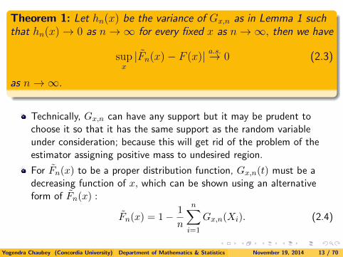
Theorem 1: Let hn(x) be the variance of Gx,n as in Lemma 1 suchthat hn(x)→ 0 as n→∞ for every fixed x as n→∞, then we have

supx|Fn(x)− F (x)|

a.s.→ 0 (2.3)

as n→∞.

Technically, Gx,n can have any support but it may be prudent tochoose it so that it has the same support as the random variableunder consideration; because this will get rid of the problem of theestimator assigning positive mass to undesired region.

For Fn(x) to be a proper distribution function, Gx,n(t) must be adecreasing function of x, which can be shown using an alternativeform of Fn(x) :

Fn(x) = 1− 1

n

n∑i=1

Gx,n(Xi). (2.4)


Equation (2.4) suggests a smooth density estimator given by

fn(x) =dFn(x)

dx= − 1

n

n∑i=1

d

dxGx,n(Xi). (2.5)

The potential of this lemma for smooth density estimation wasrecognized by Gawronski (1980) in his doctoral thesis written at Ulm.Gawronski and Stadmuller (1980, Skand. J. Stat.) investigated meansquare error properties of the density estimator when Gx,n is obtainedby putting Poisson weight

pk(xλn) = e−λnx(λnx)k

k!(2.6)

to the lattice points k/λn, k = 0, 1, 2, ...


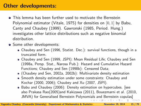
Other developments:

This lemma has been further used to motivate the BernsteinPolynomial estimator (Vitale, 1975) for densities on [0, 1] by Babu,Canty and Chaubey (1999). Gawronski (1985, Period. Hung.)investigates other lattice distributions such as negative binomialdistribution.

Some other developments:Chaubey and Sen (1996, Statist. Dec.): survival functions, though in atruncated form.Chaubey and Sen (1999, JSPI): Mean Residual Life; Chaubey and Sen(1998a, Persp. Stat., Narosa Pub.): Hazard and Cumulative HazardFunctions; Chaubey and Sen (1998b): Censored Data;(Chaubey and Sen, 2002a, 2002b): Multivariate density estimationSmooth density estimation under some constraints: Chaubey andKochar (2000, 2006); Chaubey and Xu (2007, JSPI).Babu and Chaubey (2006): Density estimation on hypercubes. [seealso Prakasa Rao(2005)and Kakizawa (2011), Bouezmarni et al. (2010,JMVA) for Generalised Bernstein Polynomials and Bernstein copulas]


A Generalised Kernel Estimator for Densities withNon-Negative Support

Lemma 1 motivates the generalised kernel estimator of Foldes andRevesz (1974):

fnGK(x) =1

n

n∑i=1

hn(x,Xi)

Chaubey et al. (2012, J. Ind. Stat. Assoc.) show the followingadaptation using asymmetric kernels for estimation of densities withnon-negative support.

Let Qv(x) represent a distribution on [0,∞) with mean 1 andvariance v2, then an estimator of F (x) is given by

F+n (x) = 1− 1

n

n∑i=1

Qvn

(Xi

x

), (2.7)

where vn → 0 as n→∞.Yogendra Chaubey (Concordia University) Department of Mathematics & Statistics November 19, 2014 16 / 70

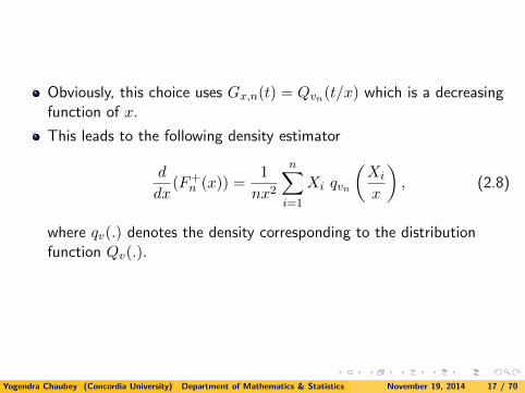
Obviously, this choice uses Gx,n(t) = Qvn(t/x) which is a decreasingfunction of x.

This leads to the following density estimator

d

dx(F+

n (x)) =1

nx2

n∑i=1

Xi qvn

(Xi

x

), (2.8)

where qv(.) denotes the density corresponding to the distributionfunction Qv(.).


However, the above estimator may not be defined at x = 0, except incases where limx→0

ddx(F+

n (x)) exists. Moreover, this limit istypically zero, which is acceptable only when we are estimating adensity f with f(0) = 0.

Thus with a view of the more general case where 0 ≤ f(0) <∞, weconsidered the following perturbed version of the above densityestimator:

f+n (x) =1

n(x+ εn)2

n∑i=1

Xi qvn

(Xi

x+ εn

), x ≥ 0 (2.9)

where εn ↓ 0 at an appropriate (sufficiently slow) rate as n→∞. Inthe sequel, we illustrate our method by taking Qv(.) to be theGamma (α = 1/v2, β = v2) distribution function.


Remark:

Note that if we believe that the density is zero at zero, we set εn ≡ 0,however in general, it may be determined using the cross-validationmethods. For εn > 0, this modification results in a defective distributionF+n (x+ εn). A corrected density estimator f∗n(x) is therefore proposed:

f∗n(x) =f+n (x)

cn, (2.10)

where cn is a constant given by

cn =1

n

n∑i=1

Qvn

(Xi

εn

).

Note that, since for large n, εn → 0, f∗n(x) and f+n (x) are asymptoticallyequivalent, we study the asymptotic properties of f+n (x) only.


Next we present a comparison of our approach with some existingestimators.

Kernel Estimator.

The usual kernel estimator is a special case of the representationgiven by Eq. (2.5), by taking Gx,n(.) as

Gx,n(t) = K

(t− xh

), (2.11)

where K(.) is a distribution function with mean zero and variance 1.


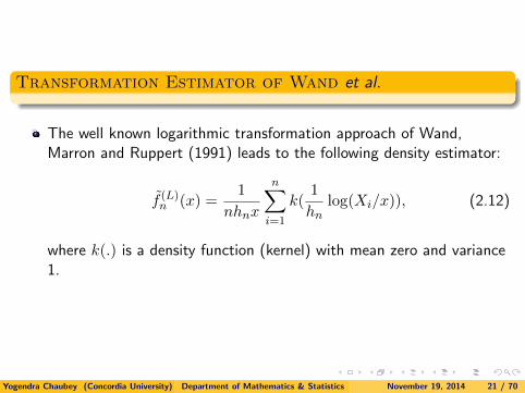
Transformation Estimator of Wand et al.

The well known logarithmic transformation approach of Wand,Marron and Ruppert (1991) leads to the following density estimator:

f (L)n (x) =1

nhnx

n∑i=1

k(1

hnlog(Xi/x)), (2.12)

where k(.) is a density function (kernel) with mean zero and variance1.


This is easily seen to be a special case of Eq. (2.5), taking Gx,n againas in Eq. (2.11) but applied to log x. This approach, however, createsproblem at the boundary which led Marron and Ruppert (1994) topropose modifications that are computationally intensive.

Estimators of Chen and Scaillet.

Chen’s (2000) estimator is of the form

fC(x) =1

n

n∑i=1

gx,n(Xi), (2.13)

where gx,n(.) is the Gamma(α = a(x, b), β = b) density with b→ 0and ba(x, b)→ x.


This also can be motivated from Eq. (2.1) as follows: takeu(t) = f(t) and note that the integral

∫f(t)gx,n(t)dt can be

estimated by n−1∑n

i=1 gx,n(Xi). This approach controls theboundary bias at x = 0; however, the variance blows up at x = 0, andcomputation of mean integrated squared error (MISE) is nottractable. Moreover, estimators of derivatives of the density are noteasily obtainable because of the appearance of x as argument of theGamma function.


Scaillet’s (2004) estimators replace the Gamma kernel by inverseGaussian (IG) and reciprocal inverse Gaussian (RIG) kernels. Theseestimators are more tractable than Chen’s; however, the IG-kernelestimator assumes value zero at x = 0, which is not desirable whenf(0) > 0, and the variances of the IG as well as the RIG estimatorsblow up at x = 0.

Bouezmarni and Scaillet (2005), however, demonstrate goodfinite-sample performance of these estimators.


It is interesting to note that one can immediately define aChen-Scaillet version of our estimator, namely,

f+n,C(x) =1

n

n∑i=1

1

xqvn

(Xi

x

).

On the other hand, our version (i.e., perturbed version) this estimatorwould be

f+C (x) =1

n

n∑i=1

gx+εn,n(Xi);

that should not have the problem of variance blowing up at x = 0.


It may also be remarked that the idea used here may be extended tothe case of densities supported on an arbitrary interval[a, b], −∞ < a < b <∞, by choosing for instance a Beta kernel(extended to the interval [a, b]) as in Chen (1999). Without loss ofgenerality, suppose a = 0 and b = 1. Then we can choose, forinstance, qv(.) as the density of Y/µ, whereY ∼ Beta(α, β), µ = α/(α+ β), such that α→∞ and β/α→ 0, sothat Var(Y/µ)→ 0.


2.2 Asymptotic Properties of the New Estimator

2.2.1 Asymptotic Properties of F+n (x)

The strong consistency holds in general for the estimator F+n (x). We can

easily prove the following theorem parallel to the strong convergence of theempirical distribution function.

Theorem:

If λn →∞ as n→∞ we have

supx|F+n (x)− F (x)| a.s.→ 0.

as n→∞.


We can also show that for large n, the smooth estimator can be arbitrarilyclose to the edf by proper choice of λn, as given in the following theorem.

Theorem:Assuming that f has a bounded derivative, and λn = o(n),then for some δ > 0, we have, with probability one,

supx≥0|F+n (x)− Fn(x)| = O

(n−3/4(log n)1+δ

).


2.2.2 Asymptotic Properties of f+n (x)

Under some regularity conditions, they obtained

Theorem:

supx≥0|f+n (x)− f(x)| a.s.−→ 0

as n→∞.

Theorem:

(a) If nvn →∞, nv3n → 0, nvnε2n → 0 as n→∞, we have

√nvn(f+n (x)− f(x))→ N

(0, I2(q)

µf(x)

x2), for x > 0.

(b) If nvnε2n →∞ and nvnε

4n → 0 as n→∞, we have√

nvnε2n(f+n (0)− f(0))→ N(0, I2(q)f(0)

).


2.3. Extensions to Non-iid cases

We can extend the technique to non-iid cases where a version of Fn(x) isavailable.

Chaubey, Y.P., Dewan, I. and Li, J. (2012) – Density estimation forstationary associated sequences. Comm. Stat.- Simula. Computa.41(4), 554- 572 –Using generalised kernel approach Chaubey

Chaubey, Yogendra P., Dewan, Isha and Li, Jun (2011) – Densityestimation for stationary associated sequences using Poisson weights.Statist. Probab. Lett. 81, 267-276.

Chaubey, Y.P. and Dewan, I. (2010). A review for smooth estimationof survival and density functions for stationary associated sequences:Some recent developments – J. Ind. Soc. Agr. Stat. 64(2), 261-272.

Chaubey, Y.P., Laıb, N. and Sen, A. (2010). Generalised kernelsmoothing for non-negative stationary ergodic processes – Journal ofNonparametric Statistics, 22, 973-997


3. Estimation of Density in Length-biased Data

In general, when the probability that an item is sampled isproportional to its size, size biased data emerges.

The density g of the size biased observation for the underlying densityf, is given by

g(x) =w(x)f(x)

µw, x > 0, (3.1)

where w(x) denotes the size measure and µw =∫w(x)f(x).

In the area of forestry, the size measure is usually proportional toeither length or area (see Muttlak and McDonald, 1990).

Another important application occurs in renewal theory whereinter-event times data are of this type if they are obtained bysampling lifetimes in progress at a randomly chosen point in time (seeCox, 1969).


Here we will talk about the length biased case where we can write

f(x) =1

xg(x)/µ. (3.2)

In principle any smooth estimator of the density function g may betransformed into that of the density function f as follows:

f(x) =1

xg(x)/µ, (3.3)

where µ is an estimator of µ.

Note that 1/µ = Eg(1/X), hence a strongly consistent estimator of µis given by

µ = n{n∑i=1

X−1i }−1


Bhattacharyya et al. (1988) used this strategy in proposing thefollowing smooth estimator of f,

fB(x) = µ(nx)−1n∑i=1

kh(x−Xi). (3.4)

Also since, F (x) = µ Eg(X−11(X≤x)), Cox (1969) proposed the

following as an estimator of the distribution function F (x) :

Fn(x) = µ1

n

n∑i=1

X−1i 1(Xi≤x). (3.5)

So there are two competing strategies for density estimation for LBdata. One is to estimate g(x) and then use the relation (3.3) (i.e.smooth Gn as in Bhattacharyya et al. (1988)). The other is tosmooth the Cox estimator Fn(x) directly and use the derivative as thesmooth estimator of f(x).


Jones (1991) studied the behaviour of the estimator fB(x) in contrastto smooth estimator obtained directly by smoothing the estimatorFn(x), by Kernel method:

fJ(x) = n−1µ

n∑i=1

X−1i kh(x−Xi). (3.6)

He noted that this estimator is a proper density function whenconsidered with the support on the whole real line, where as fB(y)may be not. He compared the two estimators based on simulations,and using the asymptotic arguments, concluded that the latterestimator may be preferable in practical applications.

Also using Jensen’s inequality we find that

Eg(µ) ≥ 1/Eg{1

n

n∑i=1

X−1i } = µ,

hence the estimator µ may be positively biased which would transferinto increased bias in the above density estimators.


If g(x)/x is integrable, the deficiency of fB(x) of not being a properdensity may be corrected by considering the alternative estimator

fa(x) =g(x)/x∫

(g(x)/x)dx, (3.7)

and this may also eliminate the increase in bias to some extent.However, in these situations, since X is typically a non-negativerandom variable, the estimator must satisfy the following twoconditions:

(i) g(x) = 0 for x ≤ 0,(ii) g(x)/x is integrable.

Here both of the estimators fB(x) and fJ(x) do not satisfy theseproperties.

We have a host of alternatives, those based on smoothing Gn andthose based on smoothing Fn, that we are going to talk about next.


3.1.1 Poisson Smoothing of Gn

Here, we would like to see the application of the weights generated bythe Poisson probability mass function as motivated in Chaubey andSen (1996, 2000). However, a modification is necessary in the presentsituation which is also outlined here.

Using Poisson smoothing, an estimator of g(x) may be given by,

gnP (x) = λn

∞∑k=0

pk(λnx)

[Gn

(k + 1

λn

)−Gn

(k

λn

)], (3.8)

however, note that limx→0gnP (x) = λnGn(1/λn) which mayconverge to 0 as λn →∞, however for finite samples it may not bezero, hence the density f at x = 0 may not be defined. Furthermore,gnP (x)/x is not integrable.


A simple modification by attaching the weight pk(λnx) toGn((k − 1)/λn), rather than to Gn(k/λn), the above problem isavoided. This results in the following smooth estimator of G(x) :

Gn(x) =∑k≥0

pk(xλn)Gn

(k − 1

λn

), (3.9)

The basic nature of the smoothing estimator is not changed, howeverthis provides an alternative estimator of the density function as itsderivative is given by

gn(x) = λn∑k≥1

pk(xλn)

[Gn

(k

λn

)−Gn

(k − 1

λn

)], (3.10)

such that gn(0) = 0 and that gn(x)/x is integrable.


Since,∫ ∞0

gn(x)

xdx = λn

∑k≥1

[Gn

(k

λn

)−Gn

(k − 1

λn

)]

∫ ∞0

pk(xλn)

xdx

= λn∑k≥1

[Gn

(k

λn

)−Gn

(k − 1

λn

)]1

k

= λn∑k≥1

1

k(k + 1)Gn

(k

λn

),

The new smooth estimator of the length biased density f(x) is givenby

fn(x) =

∑k≥1

pk−1(xλn)k

[Gn

(kλn

)−Gn

(k−1λn

)]∑

k≥11

k(k+1)Gn

(kλn

) . (3.11)


The corresponding smooth estimator of the distribution functionF (x) is given by

Fn(x) =

∑k≥1(1/k)Wk(xλn)[Gn

(kλn

)−Gn

(k−1λn

)]∑

k≥11

k(k+1)Gn

(kλn

) (3.12)

where

Wk(λnx) =1

Γ(k)

∫ λnx

0e−yyk−1dy =

∑j≥k

pj(λnx).


An equivalent expression for the above estimator is given by

Fn(x) =

∑k≥1Gn

(kλn

) [Wk(λnx)

k − Wk+1(λnx)k+1

]∑

k≥11

k(k+1)Gn

(kλn

)= 1 +

∑k≥1Gn

(kλn

) [Pk(λnx)k+1 − Pk−1(λnx)

k

]∑

k≥11

k(k+1)Gn

(kλn

) ,

where Pk(µ) =

k∑j=0

pj(µ)

denotes the cumulative probability corresponding to the Poisson(µ)distribution.

The properties of above estimators can be established in an analogousway to those in the regular case.


3.1.2 Gamma Smoothing of Gn

The smooth estimator using the log-normal density may typically havea spike at zero, however the gamma density may be appropriate, sinceit typically has the density estimator g(x) such that g(0) = 0, so thatno perturbation is required. The smooth density estimator in this caseis simply given by

g+n (x) =1

nx2

n∑i=1

Xi qvn

(Xi

x

), (3.13)

where qv(.) denotes the density corresponding to aGamma(α = 1/vn, β = vn). and the corresponding estimator ofdensity is given by

f+n (x) =g+n (x)/x∫∞

0 (g+n (t)/t)dt(3.14)


3.2.1 Poisson Smoothing of Fn

smoothing Fn directly using Poisson weights, an estimator of f(x)may be given by,

fnP (x) = λn

∞∑k=0

pk(λnx)

[Fn

(k + 1

λn

)− Fn

(k

λn

)]. (3.15)

No modifications are necessary.


3.2.2 Gamma Smoothing of Fn

The gamma based smooth estimate of F (x) is given by

F+n (x) = 1−

∑ni=1

1XiQvn(Xix )∑n

i=11Xi

, (3.16)

and that for the density f in this case is simply given by

f+n (x) =

1(x+εn)2

∑ni=1 qvn( Xi

x+εn)∑n

i=11Xi

. (3.17)

where qv(.) denotes the density corresponding to aGamma(α = 1/vn, β = vn).

Note that the above estimator is computationally intensive as twosmoothing parameters have to be computed using bivariate crossvalidation.


4. A Simulation Study

Here we consider parent distributions to estimate as exponential (χ22),

χ26, lognormal, Weibull and mixture of exponential densities.

Since the computation is very extensive for obtaining the smoothingparameters, we compute approximations to MISE and MSE bycomputing

ISE(fn, f) =

∫ ∞0

[fn(x)− f(x)]2dx

andSE (fn(x), f(x)) = [fn(x)− f(x)]2

for 1000 samples.


Here, MISE give us the global performance of density estimator.MSE let us to see how the density estimator performs locally at thepoints in which we might be interested. It is no doubt that weparticularly want to know the behavior of density estimators near thelower boundary. We illustrate only MISE values.

Optimal values of smoothing parameters are obtained using eitherBCV or UCV criterion, that roughly approximates Mean IntegratedSquared Error.

For Poisson smoothing as well as for Gamma smoothing BCVcriterion is found to be better, where as for Chen and Scailletmethod, use of BCV method is not tractable as it requires estimate ofthe derivative of the density.


Next table gives the values of MISE for exponential density using newestimators as compared with Chen’s and Scaillet estimators. Notethat we include the simulation results for Scaillet’s estimator usingRIG kernel only.

Inverse Gaussian kernel is known not to perform well for direct data[see Kulasekera and Padgett (2006)]. Similar observations were notedfor LB data.


Table: Simulated MISE for χ22

Distribution EstimatorSample Size

30 50 100 200 300 500

χ22

Chen-1 0.13358 0.08336 0.07671 0.03900 0.03056 0.02554Chen-2 0.11195 0.08592 0.05642 0.03990 0.03301 0.02298RIG 0.14392 0.11268 0.07762 0.06588 0.05466 0.04734

Poisson(F) 0.04562 0.03623 0.02673 0.01888 0.01350 0.01220Poisson(G) 0.08898 0.06653 0.04594 0.03127 0.02487 0.01885Gamma(F) 0.06791 0.05863 0.03989 0.03135 0.02323 0.01589Gamma*(F) 0.02821 0.01964 0.01224 0.00796 0.00609 0.00440Gamma(G) 0.09861 0.07663 0.05168 0.03000 0.02007 0.01317Gamma*(G) 0.02370 0.01244 0.00782 0.00537 0.00465 0.00356


Table: Simulated MSE for χ22

Sample Size Estimatorx

0 0.1 1 2 5

n=30

I 0.1307 0.2040 0.0181 0.0044 0.0003II 0.1187 0.2499 0.0173 0.0045 0.0012III 0.2222 0.1823 0.0250 0.0074 0.0022IV 0.1487 0.1001 0.0049 0.0015 0.0005V 0.3003 0.2438 0.0286 0.0148 0.0013VI 0.1936 0.1447 0.0117 0.0042 0.0002

VI* 0.0329 0.0286 0.0090 0.0030 9.8 × 10−5

VII 0.1893 0.1720 0.0209 0.0066 0.0003

VII* 0.0528 0.0410 0.0032 0.0020 8.4 × 10−5

n=50

I 0.1370 0.1493 0.0121 0.0030 0.0002II 0.1279 0.1894 0.0112 0.0032 0.0008III 0.2193 0.1774 0.0161 0.0046 0.0046IV 0.1393 0.0885 0.0034 0.0012 0.0003V 0.2939 0.1924 0.0218 0.0094 0.0007VI 0.1808 0.1365 0.0101 0.0036 0.0001

VI* 0.0196 0.0172 0.0070 0.0024 6.8 × 10−5

VII 0.1584 0.1440 0.0168 0.0060 0.0002

VII* 0.0322 0.0236 0.0014 0.0012 4.8 × 10−5

I-Chen-1, II-Chen-2, III-RIG, IV-Poisson(F), V-Poisson(G), VI-Gamma(F), VI*-Corrected Gamma(F), VII-Gamma(G),VII*-Corrected Gamma(G)




0 0.1 1 2 5

n=100

I 0.1442 0.8201 0.0070 0.0017 0.0001II 0.1142 0.1391 0.0054 0.0019 0.0005III 0.2151 0.1631 0.0091 0.0030 0.0020IV 0.1335 0.0724 0.0023 0.0008 0.0002V 0.2498 0.1267 0.0116 0.0050 0.0003VI 0.1332 0.0823 0.0090 0.0032 0.0001

VI* 0.0105 0.0094 0.0047 0.0015 5.9 × 10−5

VII 0.1078 0.0980 0.0121 0.0051 0.0002

VII* 0.0280 0.0184 0.0006 0.0007 3.8 × 10−5

n=200

I 0.3327 0.0901 0.0046 0.0012 6.6 × 10−5

II 0.2111 0.0943 0.0027 0.0012 0.0003III 0.2127 0.1896 0.0067 0.0019 0.0080IV 0.1139 0.0545 0.0015 0.0005 0.0001V 0.1908 0.0703 0.0056 0.0026 0.0001

VI 0.0995 0.0782 0.0065 0.0024 7.4 × 10−5

VI* 0.0137 0.0125 0.0031 0.0010 5.8 × 10−5

VII 0.0636 0.0560 0.0072 0.0038 0.0002

VII* 0.0217 0.0134 0.0002 0.0005 2.9 × 10−5

I-Chen-1, II-Chen-2, III-RIG, IV-Poisson(F), V-Poisson(G),VI-Gamma(F), VI*-Corrected Gamma(F),VII-Gamma(G),VII*-Corrected Gamma(G)


Table: Simulated MISE for χ26


30 50 100 200 300 500

χ26

Chen-1 0.01592 0.01038 0.00578 0.00338 0.00246 0.00165Chen-2 0.01419 0.00973 0.00528 0.00303 0.00224 0.00153RIG 0.01438 0.00871 0.00482 0.00281 0.00208 0.00148

Poisson(F) 0.00827 0.00582 0.00382 0.00241 0.00178 0.00119Poisson(G) 0.00834 0.00562 0.00356 0.00216 0.00166 0.00117Gamma(F) 0.01109 0.00805 0.00542 0.00327 0.00249 0.00181Gamma*(F) 0.01141 0.00844 0.00578 0.00345 0.00264 0.00193Gamma(G) 0.01536 0.01063 0.00688 0.00398 0.00303 0.00213Gamma*(G) 0.01536 0.01063 0.00688 0.00398 0.00303 0.00213




0 0.1 1 4 10

n=30

I 0.0017 0.0018 0.0018 0.0019 0.0001II 0.0018 0.0017 0.0011 0.0017 0.0002

III 5.6 × 10−5 6.7 × 10−5 0.0006 0.0017 0.0002IV 0.0016 0.0016 0.0012 0.0012 0.0001

V 0.0000 2.6 × 10−5 0.0017 0.0008 0.0001

VI 0.0011 0.0010 0.0019 0.0012 8.5 × 10−5

VI* 0.0015 0.0021 0.0020 0.0012 7.9 × 10−5

VII 0.0000 3.6 × 10−7 0.0058 0.0008 0.0001

VII* 0.0000 3.6 × 10−7 0.0058 0.0008 0.0001

n=50

I 0.0012 0.0013 0.0015 0.0012 0.0001II 0.0013 0.0012 0.0008 0.0011 0.0001

III 4.6 × 10−5 5.7 × 10−5 0.0006 0.0005 .0001

IV 0.0011 0.0011 0.0010 0.0008 8.4 × 10−5

V 0.0000 6.7 × 10−5 0.0012 0.0005 0.0001

VI 0.0005 0.0005 0.0016 0.0008 5.5 × 10−5

VI* 0.0006 0.0015 0.0016 0.0008 5.3 × 10−5

VII 0.0000 4.3 × 10−6 0.0037 0.0004 7.9 × 10−5

VII* 0.0000 4.3 × 10−6 0.0037 0.0004 7.9 × 10−5

I-Chen-1, II-Chen-2, III-RIG, IV-Poisson(F), V-Poisson(G), VI-Gamma(F), VI*-Corrected Gamma(F), VII-Gamma(G),VII*-Corrected Gamma(G)


For the exponential density, fC2 has smaller MSEs at the boundaryand MISEs than fC1. This means fC2 performs better locally andglobally than fC1. Similar result holds in direct data.

Poisson weight estimator based on Fn is found to be better than thatbased on Gn.

Although Poisson weight estimator based on Gn has relatively smallerMISEs, it has large MSEs at the boundary as well, just like Scailletestimator.

Scaillet estimator has huge MSEs at the boundary and the largestMISEs.

Corrected Gamma estimators have similar and smaller MISE values ascompared to the corresponding Poisson weight estimators.

For χ26, all estimators have comparable global results. Poison weight

estimators based on Fn or Gn have similar performances and may beslightly better than the others.


We have considered following additional distributions for simulation as well:(i). Lognormal Distribution

f(x) =1√2πx

exp{−(log x− µ)2/2}I{x > 0};

(ii). Weibull Distribution

f(x) = αxα−1 exp(−xα)I{x > 0};

(iii). Mixtures of Two Exponential Distribution

f(x) = [π1

θ1exp(−x/θ1) + (1− π)

1

θ2exp(−x/θ2]I{x > 0}.


Table: Simulated MISE for Lognormal with µ = 0


30 50 100 200 300 500

Lognormal

Chen-1 0.12513 0.08416 0.05109 0.03450 0.02514 0.01727Chen-2 0.12327 0.08886 0.05200 0.03545 0.02488 0.01717RIG 0.14371 0.09733 0.05551 0.03308 0.02330 0.01497

Poisson(F) 0.05559 0.04379 0.02767 0.01831 0.01346 0.01001Poisson(G) 0.06952 0.04820 0.03158 0.01470 0.01474 0.01061Gamma*(F) 0.06846 0.05614 0.03963 0.02640 0.01998 0.01470Gamma*(G) 0.16365 0.12277 0.07568 0.04083 0.029913 0.02035


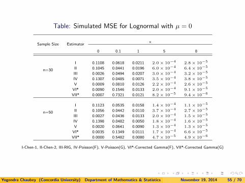
Table: Simulated MSE for Lognormal with µ = 0


0 0.1 1 5 8

n=30

I 0.1108 0.0618 0.0211 2.0 × 10−4 2.8 × 10−5

II 0.1045 0.0441 0.0196 6.0 × 10−4 6.4 × 10−5

III 0.0026 0.0494 0.0207 3.0 × 10−4 3.2 × 10−5

IV 0.1307 0.0485 0.0071 3.5 × 10−4 3.8 × 10−5

V 0.0009 0.0810 0.0126 2.2 × 10−4 2.6 × 10−5

VI* 0.0090 0.1546 0.0133 2.0 × 10−4 9.1 × 10−5

VII* 0.0007 0.7321 0.0121 8.2 × 10−5 9.4 × 10−6

n=50

I 0.1123 0.0535 0.0158 1.4 × 10−4 1.1 × 10−5

II 0.1056 0.0442 0.0110 3.7 × 10−4 2.7 × 10−5

III 0.0027 0.0436 0.0133 2.0 × 10−4 1.5 × 10−5

IV 0.1398 0.0482 0.0050 1.8 × 10−4 1.6 × 10−5

V 0.0020 0.0641 0.0090 1.3 × 10−4 1.3 × 10−5

VI* 0.0035 0.1349 0.0111 1.7 × 10−4 6.6 × 10−5

VII* 0.0000 0.5482 0.0080 4.7 × 10−5 4.9 × 10−6

I-Chen-1, II-Chen-2, III-RIG, IV-Poisson(F), V-Poisson(G), VI*-Corrected Gamma(F), VII*-Corrected Gamma(G)


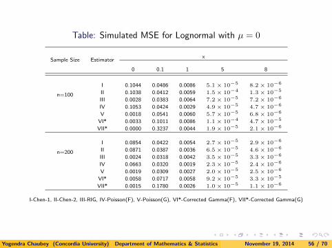
Table: Simulated MSE for Lognormal with µ = 0


0 0.1 1 5 8

n=100

I 0.1044 0.0486 0.0086 5.1 × 10−5 8.2 × 10−6

II 0.1038 0.0412 0.0059 1.5 × 10−4 1.3 × 10−5

III 0.0028 0.0383 0.0064 7.2 × 10−5 7.2 × 10−6

IV 0.1053 0.0424 0.0029 4.9 × 10−5 4.7 × 10−6

V 0.0018 0.0541 0.0060 5.7 × 10−5 6.8 × 10−6

VI* 0.0033 0.1011 0.0086 1.1 × 10−4 4.7 × 10−5

VII* 0.0000 0.3237 0.0044 1.9 × 10−5 2.1 × 10−6

n=200

I 0.0854 0.0422 0.0054 2.7 × 10−5 2.9 × 10−6

II 0.0871 0.0387 0.0036 6.5 × 10−5 4.6 × 10−6

III 0.0024 0.0318 0.0042 3.5 × 10−5 3.3 × 10−6

IV 0.0663 0.0320 0.0019 2.3 × 10−5 2.4 × 10−6

V 0.0019 0.0309 0.0027 2.0 × 10−5 2.5 × 10−6

VI* 0.0058 0.0717 0.0058 9.2 × 10−5 3.3 × 10−5

VII* 0.0015 0.1780 0.0026 1.0 × 10−5 1.1 × 10−6



Table: Simulated MISE for Weibull with α = 2


30 50 100 200 300 500

Weibull

Chen-1 0.10495 0.06636 0.03884 0.02312 0.01700 0.01167Chen-2 0.08651 0.05719 0.03595 0.02225 0.01611 0.01111RIG 0.08530 0.05532 0.03227 0.01984 0.01470 0.01045



Table: Simulated MSE for Weibull with α = 2


0 0.1 1 2 3

n=30

I 0.0856 0.1343 0.0588 .0030 1.9 × 10−4

II 0.0949 0.0555 0.0398 .0116 1.4 × 10−4

III 0.0025 0.0802 0.0394 .0095 4.6 × 10−4

IV 0.0844 0.0548 0.0280 0.0086 6.9 × 10−4

V 0.0068 0.0636 0.0186 0.0031 3.1 × 10−5

VI* 0.0019 0.1049 0.0682 0.0053 0.0022

VII* 0.0000 0.2852 0.0336 0.0011 1.8 × 10−4

n=50

I 0.0644 0.0576 0.0349 0.0020 1.0 × 10−4

II 0.0679 0.0431 0.0223 0.0077 7.1 × 10−4

III 0.0021 0.0208 0.0218 0.0063 2.2 × 10−4

IV 0.0682 0.0427 0.0217 0.0059 3.7 × 10−4

V 0.0025 0.0453 0.0138 0.0018 1.6 × 10−5

VI* 1.1 × 10−6 0.0763 0.0560 0.0048 0.0018

VII* 0.0000 0.1865 0.0251 0.0008 1.4 × 10−4



Table: Simulated MISE for Mixture of Two Exponential Distributions withπ = 0.4, θ1 = 2 and θ2 = 1


30 50 100 200 300 500

Mixture

Chen-1 0.22876 0.17045 0.08578 0.06718 0.05523 0.03811Chen-2 0.17564 0.15083 0.07331 0.08029 0.04931 0.03808RIG 0.25284 0.20900 0.13843 0.10879 0.09344 0.07776



Table: Simulated MSE for Mixtures of Two Exponential Distributions withπ = 0.4, θ1 = 2 and θ2 = 1


0 0.1 1 2 10

n=30

I 0.3499 0.3075 0.0249 0.0037 2.6 × 10−6

II 0.3190 0.3181 0.0245 0.0071 1.3 × 10−5

III 0.5610 0.4423 0.0564 0.0056 2.9 × 10−6

IV 0.3778 0.1907 0.0057 0.0027 1.7 × 10−6

V 0.6409 0.3237 0.0156 0.0043 2.1 × 10−6

VI* 0.0652 0.0549 0.0098 0.0006 1.1 × 10−4

VII* 0.0696 0.0539 0.0065 0.0009 1.4 × 10−5

n=50

I 0.3158 0.7921 0.0128 0.0023 1.1 × 10−6

II 0.2848 0.7600 0.0143 0.0051 2.3 × 10−6

III 0.5582 0.8473 0.0364 0.0041 1.3 × 10−6

IV 0.3840 0.1633 0.0051 0.0020 1.0 × 10−6

V 0.6228 0.2673 0.0121 0.0028 1.3 × 10−6

VI* 0.0489 0.0414 0.0066 0.0004 7.7 × 10−5

VII* 0.0500 0.0336 0.0030 0.0007 9.2 × 10−6



The basic conclusion is that the smoothing based on Fn usingPoisson weights or corrected Gamma perform in a similar way andproduce better boundary correction as compared to Chen or Scailletasymmetric kernel estimators.

The smoothing based on Gn may have large local MSE near theboundary and hence is not preferable over smoothing of Fn. A similarmessage is given in Jones and Karunamuni (1997, Austr. J. Stat.).


References

Babu, G.J., Canty, A.J. and Chaubey, Y.P.(2002). Application ofBernstein polynomials for smooth estimation of a distribution anddensity function. J. Statist. Plann. Inference 105, no. 2, 377-392.

Babu, G.J. and Chaubey, Yogendra P. (2006). Smooth estimation ofa distribution and density function on a hypercube using Bernsteinpolynomials for dependent random vectors. Statistics & ProbabilityLetters 76 959-969.

Bagai, I. and Prakasa Rao, B.L.S. (1996). Kernel Type DensityEstimates for Positive Valued Random Variables. Sankhya A5756–67.

Bhattacharyya, B.B., L.A. Franklin, G.D. Richardson (1988). Acomparison of nonparametric unweighted and length biased densityestimation of fibres.Communications in Statistics- Theory Method17(11) 3629–3644.


Bouezmarni, T., Rombouts, J.V.K. and Taamouti, A. (2010).Asymptotic Properties of the Bernstein Density Copula for DependentData. Journal of Multivariate Analysis, 101, 1-10.

Bouezmarni, T. and Scaillet, O. (2005). Consistency of AsymmetricKernel Density Estimators and Smoothed Histograms withApplication to Income Data. Econometric Theory, 21, 390-412.

Chaubey, Y.P. and Kochar, S. (2000). Smooth estimation ofstochastically ordered Survival functions. J. Indian StatisticalAssociation, 38, 209-225.

Chaubey, Yogendra P. and Kochar, Subhash C. (2006). Smoothestimation of uniformly stochastically ordered survival functions.Journal of Combinatorics, Information and System Sciences, 31 1-13.

Chaubey, Y. P. and Sen, P. K. (1996). On Smooth Estimation ofSurvival and Density Function. Statistics and Decision, 14, 1-22.


Chaubey, Y.P., Sen, P.K. (1998a). On smooth estimation of hazardand cumulative hazard functions. In Frontiers of Probability andStatistics, S.P. Mukherjee et al. (eds.) Narosa: New Delhi; 91–99.Chaubey, Y. P. and Sen, P. K. (1998b). On Smooth FunctionalEstimation under Random Censorship. In Frontiers in Reliability 4.Series on Quality, Reliability and Engineering Statistics (A. P. Basu etal., eds.), 83-97. World Scientific, Singapore.Chaubey Y.P. and Sen P. K. (1999). On smooth estimation of meanresidual life. Journal of Statistical Planning and Inference 75 223–236.Chaubey Y.P. and Sen, P.K. (2002a). Smooth isotonic estimation ofdensity, hazard and MRL functions. Calcutta Statistical AssociationBulletin, 52, 99-116.Chaubey, Y. P. and Sen, P. K. (2002b). Smooth estimation ofMultivariate Survival and Density Functions. Jour. Statist. Plann.and Inf., 103, 361-376.Chaubey, Y. P. , Sen, A. and Sen, P. K. (2007a). A New SmoothDensity Estimator for Non-Negtive Random Variables. TechnicalReport No. 01/07, Department of Mathematics and Statistics,Concordia University, Montreal.Chaubey, Yogendra P. and Xu, Haipeng (2007b) Smooth estimationof survival functions under mean residual life ordering. Jour. Statist.Plann. Inf. 137, 3303-3316.


Chaubey, Y. P. and Sen, P. K. (2009). On the Selection ofSmoothing Parameter in Poisson Smoothing of Histogram Estimator:Computational Aspects. Pak. J. Statist., 25(4), 385-401.

Chaubey, Y. P. , Sen, P. K. and Li, J. (2010a). Smooth DensityEstimation for Length Biased Data. Journal of the Indian Society ofAgricultural Statistics, 64(2), 145-155.

Chaubey, Y.P. and Dewan, I. and Li, J. (2010b). Smooth estimationof survival and density functions for a stationary associated processusing Poisson weights Statistics and Probability Letters, 81, 267-276.

Chaubey, Y. P. , Sen, A., Sen, P. K. and Li, J. (2012). A NewSmooth Density Estimator for Non-Negative Random Variables.Journal of the Indian Statistical Association 50, 83-104.


Chen, S. X. (1999). Beta kernel estimators for density functions.Computational Statistics and Data Analysis, 31, 131–145.

Chen, S. X. (2000). Probability Density Function Estimation UsingGamma Kernels. Annals of the Institute of Statistical Mathematics,52, 471-480.

Cox, D.R. (1969). Some Sampling Problems in Technology. In NewDevelopments in Survey Sampling, U. L. Johnson and H. Smith(eds.), New York: Wiley Interscience.

Feller, W. (1965). An Introduction to Probability Theory and ItsApplications, Vol. II. New York: Wiley.

Foldes, A. and Reve, P. (1974). A general method for densityestimation. Studia Sci. Math. Hungar. (1974), 8192.


Gawronski, W. (1980). Verallgemeinerte Bernsteinfunktionen undSchtzung einer Wahrscheinlichkeitsdichte, Universitat Ulm,(Habilitationsschrift).

Gawronski, W. (1985). Strong laws for density estimators ofBernstein type. Periodica Mathematica Hungarica 16, 23-43

Gawronski, W. and Stadmuler, U. (1980). On Density Estimation byMeans of Poisson’s Distribution. Scandinavian Journal of Statistics,7, 90-94.

Gawronski, W. and Stadmuler, U. (1981). Smoothing of Histogramsby Means of Lattice and Continuous Distributions. Metrika, 28,155-164.

Jones, M.C. (1991). Kernel density estimation for length biased data.Biometrika 78 511–519.


Jones, M.C. and Karunamuni, R.J. (1997). Fourier series estimationfor length biased data. Australian Journal of Statistics, 39, 5768.

Kakizawa, Y. (2011). A note on generalized Bernstein polynomialdensity estimators. Statistical Methodology, 8, 136-153.

Kulasekera, K. B. and Padgett, W. J. (2006). Bayes BandwidthSelection in Kernel Density Estimation with Censored Data. Journalof Nonparametric Statistics, 18, 129-143.

Marron, J. S., Ruppert, D. (1994). Transformations to reduceboundary bias in kernel density estimation. J. Roy. Statist. Soc. Ser.B 56, 653-671.

Muttlak, H.A. and McDonald, L.L. (1990). Ranked set sampling withsize-biased sampling with applications to wildlife populations andhuman families. Biometrics 46, 435-445.


Prakasa Rao, B. L. S. (1983). Nonparametric Functional Estimation.Academic Press:New York.

Prakasa Rao, B. L. S. (2005). Estimation of distributions and densityfunctions by generalized Bernstein polynomials. Indian J. Pure and AppliedMath. 36, 63-88.

Rosenblatt, M. (1956). Remarks on some nonparametric estimates ofdensity functions. Ann.Math. Statist. 27 832–837.

Scaillet, O. (2004). Density Estimation Using Inverse and Reciprocal InverseGaussian Kernels. Journal of Nonparametric Statistics, 16, 217-226.

Silverman, B. W. (1986). Density Estimation for Statistics and DataAnalysis. Chapman and Hall: London.

Vitale, R. A. (1975). A Bernstein polynomial approach to densityestimation. In Statistical Inference and Related Topics (ed. M. L. Puri), 287–100. New York: Academic Press.

Wand, M.P., Marron, J.S. and Ruppert, D. (1991). Transformations in

density estimation. Journal of the American Statistical Association, 86,

343-361.


Talk slides are available on SlideShare:

http://www.slideshare.net/YogendraChaubey/talk-slides-isi2014

THANKS!!


talk slides at isi, 2014

Education