Talk 2: “Quantized Yang-Mills (d=2) and theSegal-Bargmann-Hall Transform”

Bruce DriverDepartment of Mathematics, 0112University of California at San Diego, USA

http://math.ucsd.edu/∼bdriver

Nelder Talk 2.

1pm-2:30pm, Wednesday 5th November, Room 139, Huxley

Imperial College, London

Gaussian Measures on Hilbert spaces

Goal: Given a Hilbert space H , we would ideally like to define a probability measure µon B(H) such that

µ(h) :=

∫H

ei(λ,x)dµ(x) = e−12‖λ‖

2

for all λ ∈ H (1)

so that, informally,

dµ (x) =1

Ze−

12|x|

2HDx. (2)

The next proposition shows that this is impossible when dim(H) =∞.Proposition 1. Suppose that H is an infinite dimensional Hilbert space. Then there is noprobability measure µ on the Borel σ – algebra, B = B(H), such that Eq. (1) holds.

Proof: Suppose such a Gaussian measure were to exist. If ei∞i=1 is an ON basis for H,then 〈ei, ·〉∞i=1 would be i.i.d. normal random variables. By SSLN,

limN→∞

1

N

N∑i=1

〈ei, ·〉2 = 1 µ – a.s.

Bruce Driver 2

which would imply

∞ > ‖x‖2 =

∞∑i=1

〈ei, x〉2 =∞ a.s.

Q.E.D.

Moral: The measure µ must be defined on a larger space. This is somewhat analogousto trying to define Lebesgue measure on the rational numbers. In each case the measurecan only be defined on a certain completion of the naive initial space.

Bruce Driver 3

A Non-Technicality

Theorem 2. Let Q be the rational numbers.

1. There is no translation invariant measure (m) on Q which is finite on bounded sets.

2. Similarly there is no measure (m) on Q such thatm (x ∈ Q : a < x < b) = b− a.

Proof: In either case one shows that m (r) = 0 and then by countable additivity

m (Q) =∑r∈Q

m (r) = 0.

For example if m existed as in item 2., then m (r) ≤ b− a for any choice of a < r < bwhich can only be if m (r) = 0. Q.E.D.

MORAL: To construct desirable countably additive measures the underlying set must besufficiently “big.”

Bruce Driver 4

Measures on Hilbert SpacesTheorem 3. Suppose that H and K are separable Hilbert spaces, H is a densesubspace of K, and the inclusion map, i : H → K is continuous. Then there exists aGaussian measure, ν, on K such that∫

K

eλ(x)dν (x) = exp

(1

2(λ, λ)H∗

)for all λ ∈ K∗ ⊂ H∗ (3)

iff i : H → K is Hilbert Schmidt. Recalling the Hilbert Schmidt norm of i and its adjoint,i∗, are the same, the following conditions are equivalent;

1. i : H → K is Hilbert Schmidt,

2. i∗ : K → H is Hilbert Schmidt,

3. tr (i i∗) <∞

4. tr (i∗i) <∞.

Proof: We only prove here; if i : H → K is Hilbert Schmidt, then there exists a measureν on K such that Eq. (3) holds. For the converse direction, see[Bogachev, 1998, Da Prato & Zabczyk, 1992, Kuo, 1975].

Bruce Driver 5

• A := i∗i : H → H, is a self-adjoint trace class operator.

• By the spectral theorem, there exists an orthonormal basis, ej∞j=1 for H such thatAej = ajej with aj > 0 and

∑∞j=1 aj <∞.

• (ej, ek)K = (iej, iek)K = (i∗iej, ek)H = (Aej, ek)H = ajδjk.

• Let Nj∞j=1 be i.i.d. standard normal random variables and set

S :=

∞∑j=1

Njej.

• Notice that

E[‖S‖2

K

]=

∞∑j=1

‖ej‖2K =

∞∑j=1

aj <∞

• Now take ν = Law (S) .

Q.E.D.

Bruce Driver 6

Wiener Measure Example

Example 1 (Wiener measure). Let

H =

h : [0, T ]→ Rd|h (0) = 0 and 〈h, h〉H =

∫ 1

0

|h′(s)|2ds <∞.

and take K = L2([0, T ] ,Rd

). On then shows;

1. (i∗f ) (τ ) =∫ T

0min (t, τ ) f (τ ) dτ

2. tr (i i∗) = d ·∫ T

0min (t, t) dt = d · T 2/2 <∞.

Bruce Driver 7

Euclidean Free FieldDefinition 4. For f ∈ C∞

(Td), let

‖f‖2s :=

⟨(−∆ + m2

)sf, f⟩

=∥∥∥(−∆ + m2

)s/2f∥∥∥2

L2

and set Hs be the closure inside of[C∞(Td)]′

. [We normalize Lebesgue measure tohave volume 1 on Td.]

Theorem 5. The measure,

dµ (ϕ) =1

Ze−∫Td[

12|∇ϕ(x)|2+m2ϕ2(x)]dxDϕ

exists on Hs iff s < 1− d2.

Proof: For n ∈ Zd, let χn (θ) := ein·θ for θ ∈ Td. Then

〈χn, χm〉s =⟨(−∆ + m2

)sχn, χm

⟩=[|n|2 + m2

]sδmn.

Therefore, χn√|n|2 + m2

n∈Zd

is an ON basis for H1.

Bruce Driver 8

The result now follows since

∑n∈Zd

∥∥∥∥∥∥∥χn√|n|2 + m2

∥∥∥∥∥∥∥2

s

=∑n∈Zd

1(|n|2 + m2

)1−s

which is finite iff 2 (1− s) > d ⇐⇒ s < 1− d2. Q.E.D.

Bruce Driver 9

Stochastic Quantization (Skipped)

Let V be a nice potential,

H = −1

2∆ + V,

λ0 = inf σ(H) and Ω > 0 3 HΩ = λ0Ω.

By making sense of

dµ(ω) =1

Ze−∫∞−∞12(ω′(s))2+V (ω(s))ds Dω (4)

We learn knowledge of Ω and H := Ω−1(H − λ0)Ω via:∫W

f (ω(0))dµ(ω) =

∫Ω2(x)f (x)dx

∫W

f (ω(0))g(ω(t))dµ(ω) =(et(H−λ0)Ωf,Ωg

)L2(dx)

=(etHf, g,

)L2(Ω2dx)

Bruce Driver 10

Quantized Non-Linear Klein-Gordon Equation(Skipped)

ϕtt + (−∆ + m2)ϕ + ϕ3 = 0

where ϕ : R×Rd → R. Equivalently,

ϕtt = −∇V (ϕ)

where

V (ϕ) =

∫Rd

(1

2|∇ϕ|2 +

m2

2ϕ2 +

1

4ϕ4

)dx.

Quantization leads to the equation

∂tu(t, ϕ) =1

2∆Hu(t, ϕ)− V (ϕ)u(t, ϕ)

where H := L2(Rd) with formal path integral quantization:

eT(12∆H−V )f (ϕo) =

1

ZT

∫ϕ(0)=ϕ0

e−∫ T0 [12‖ϕ(t)‖2H+V (ϕ(t))]dtf (ϕ(T ))Dϕ.

See Glimm and Jaffe’s Book, 1987.

Bruce Driver 11

The appearance of infinities

For “interacting” quantum field theories one would like to make sense of

dµv (ϕ) :=1

Ze−∫Td[

12|∇ϕ(x)|2+m2ϕ2(x)+v(ϕ(x))]dxDϕ

where v (s) is a polynomial in s like v (s) = s4. The obvious way to do this is to write,

dµv (ϕ) := e−∫Td v(ϕ(x))dx 1

Ze−∫Td[

12|∇ϕ(x)|2+m2ϕ2(x)]dxDϕ

=1

Zve−∫Td v(ϕ(x))dx · dµ0 (ϕ)

where dµ0 (ϕ) is given in Theorem 5. However, µ0 is only supported on H1−d2−ε

– aspace of distributions and therefore v (ϕ (x)) is not well defined!

Bruce Driver 12

Path IntegralQuantized Yang-Mills Fields (Skipped)

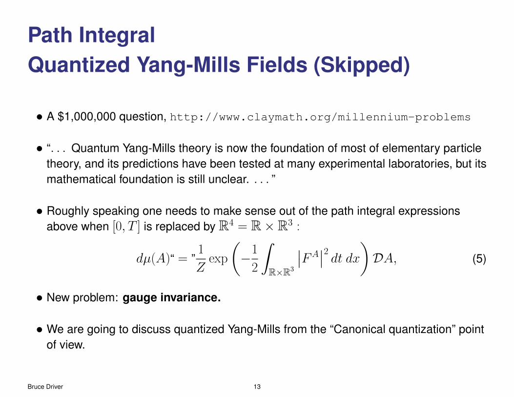
• A $1,000,000 question, http://www.claymath.org/millennium-problems

• “. . . Quantum Yang-Mills theory is now the foundation of most of elementary particletheory, and its predictions have been tested at many experimental laboratories, but itsmathematical foundation is still unclear. . . . ”

• Roughly speaking one needs to make sense out of the path integral expressionsabove when [0, T ] is replaced by R4 = R×R3 :

dµ(A)“ = ”1

Zexp

(−1

2

∫R×R3

∣∣FA∣∣2 dt dx)DA, (5)

• New problem: gauge invariance.

• We are going to discuss quantized Yang-Mills from the “Canonical quantization” pointof view.

Bruce Driver 13

Gauge Theory Notation

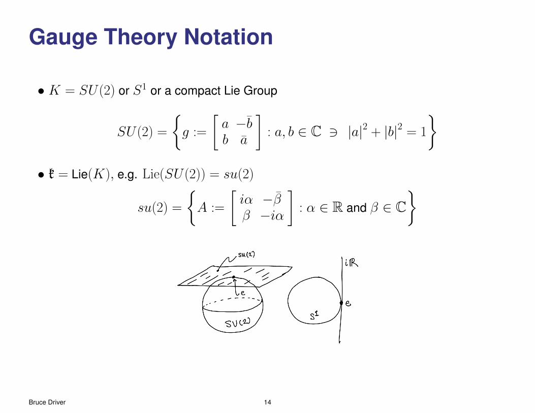
• K = SU(2) or S1 or a compact Lie Group

SU(2) =

g :=

[a −bb a

]: a, b ∈ C 3 |a|2 + |b|2 = 1

• k = Lie(K), e.g. Lie(SU(2)) = su(2)

su(2) =

A :=

[iα −ββ −iα

]: α ∈ R and β ∈ C

Bruce Driver 14

• Lie bracket: [A,B] = AB −BA =: adAB

• 〈A,B〉 = −tr(AB) = tr(A∗B)(a fixed Ad – K – invariant inner product)

•M = Rd or T d =(S1)d

.

• A = L2(M, kd) – the space of connection 1-forms.

• For A ∈ A and 1 ≤ i, k ≤ d, let

∇Ak := ∂k + adAk

(covariant differential)and

FAki := ∂kAi − ∂iAk + [Ak, Ai] (Curvature of A)

Bruce Driver 15

Newton Form of the Y. M. Equations

Define the potential energy functional, V (A) , by

V (A) :=1

2

∫Rd

∑1≤j<k≤d

|FAj,k(x)|2dx.

Then the dynamics equation may be written in Newton form as

A (t) = − (gradAV ) (A) .

The conserved energy is thus

Energy(A, A

)=

1

2

∥∥A∥∥2

A + V (A) . (6)

The weak form of the constraint equation,

0 = ∇A · E =

d∑k=1

∇AkEk is

0 =(E,∇Ah

)A ∀ h ∈ C

∞c (M, k) .

Bruce Driver 16

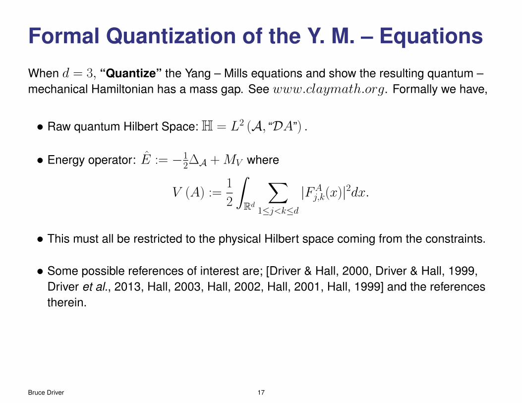
Formal Quantization of the Y. M. – Equations

When d = 3, “Quantize” the Yang – Mills equations and show the resulting quantum –mechanical Hamiltonian has a mass gap. See www.claymath.org. Formally we have,

• Raw quantum Hilbert Space: H = L2 (A, “DA”) .

• Energy operator: E := −12∆A + MV where

V (A) :=1

2

∫Rd

∑1≤j<k≤d

|FAj,k(x)|2dx.

• This must all be restricted to the physical Hilbert space coming from the constraints.

• Some possible references of interest are; [Driver & Hall, 2000, Driver & Hall, 1999,Driver et al., 2013, Hall, 2003, Hall, 2002, Hall, 2001, Hall, 1999] and the referencestherein.

Bruce Driver 17

Wilson Loop Variables

Let L = L (M) loops on M based at o ∈M.

Definition 6. Let //A (σ) ∈ K be parallel translation along σ ∈ L, that is//A (σ) := //A1 (σ) , where

d

dt//At (σ) +

d∑i=1

σi (t)Ai (σ (t)) //At (σ) = 0 with //A0 (σ) = id.

[Very ill defined unless d = 1!!]

• Physical quantum Hilbert Space

Hphysical =F ∈ L2(A,DA) : F = F

(//A (σ) : σ ∈ L

)

Bruce Driver 18

Restriction to d = 1

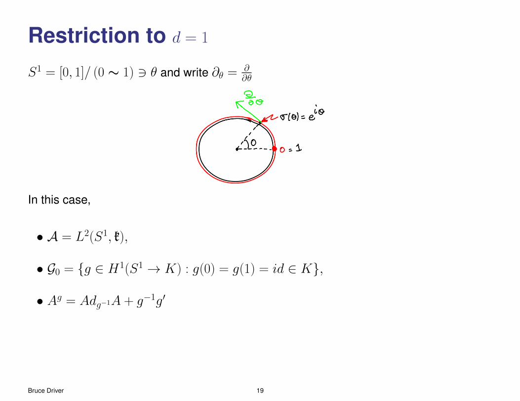
S1 = [0, 1]/ (0 ∼ 1) 3 θ and write ∂θ = ∂∂θ

In this case,

• A = L2(S1, k),

• G0 = g ∈ H1(S1 → K) : g(0) = g(1) = id ∈ K,

• Ag = Adg−1A + g−1g′

Bruce Driver 19

• H =“L2(A,DA)”

• Hphysical = F ∈ H : Fϕ(A) = ϕ(//1(A)), ϕ : K → C , where //θ(A) ∈ K is thesolution to

d

dθ//θ(A) + A(θ)//θ(A) = 0 with //0(A) = id ∈ K.

//1(A) ∈ K is the holonomy of A.

• H = −12∆A (Quantum Hamiltonian)

Remark 7. FA ≡ 0 when d = 1 and therefore, V (A) ≡ 0.

Bruce Driver 20

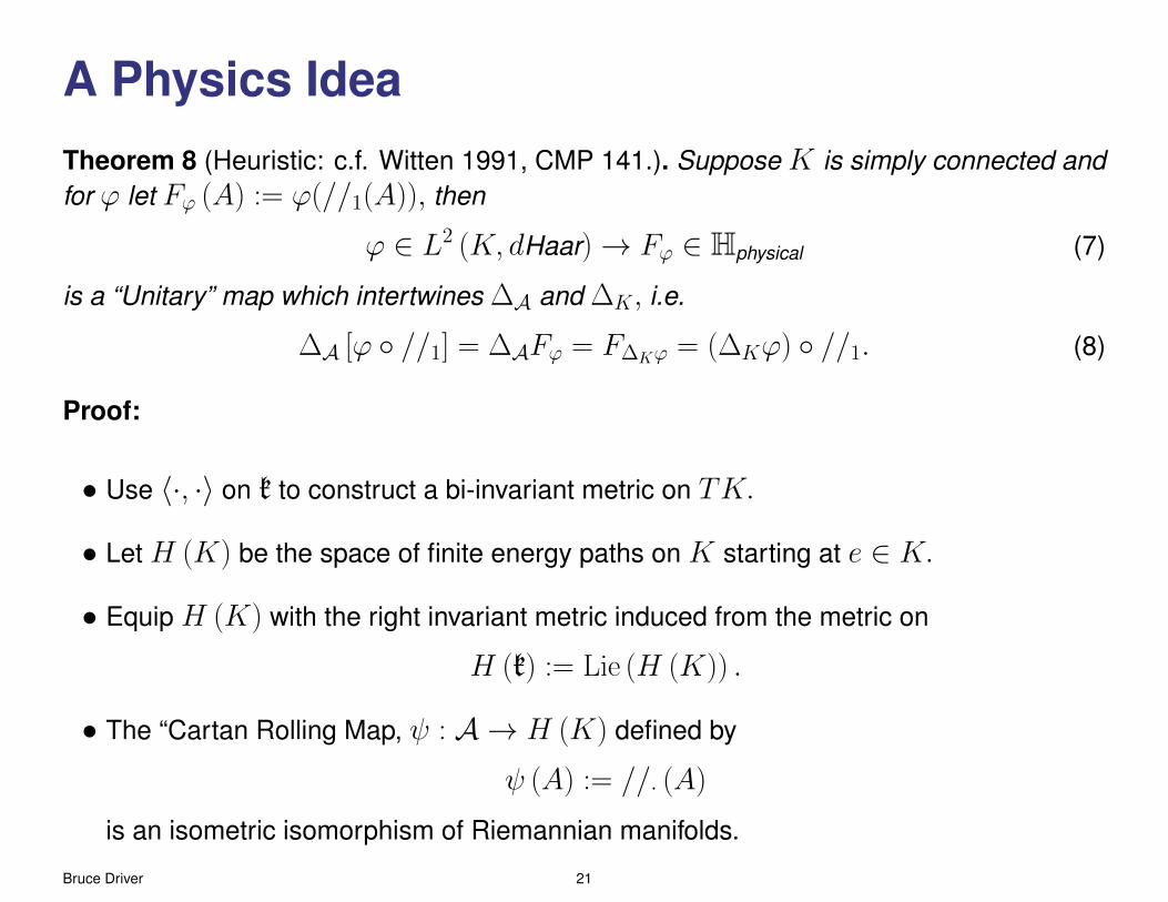
A Physics IdeaTheorem 8 (Heuristic: c.f. Witten 1991, CMP 141.). Suppose K is simply connected andfor ϕ let Fϕ (A) := ϕ(//1(A)), then

ϕ ∈ L2 (K, dHaar)→ Fϕ ∈ Hphysical (7)

is a “Unitary” map which intertwines ∆A and ∆K, i.e.

∆A [ϕ //1] = ∆AFϕ = F∆Kϕ = (∆Kϕ) //1. (8)

Proof:

• Use 〈·, ·〉 on k to construct a bi-invariant metric on TK.

• Let H (K) be the space of finite energy paths on K starting at e ∈ K.

• Equip H (K) with the right invariant metric induced from the metric on

H (k) := Lie (H (K)) .

• The “Cartan Rolling Map, ψ : A → H (K) defined by

ψ (A) := //· (A)

is an isometric isomorphism of Riemannian manifolds.

Bruce Driver 21

• Consequently we may “conclude” that ψ intertwines the Laplacian, ∆A on A with theLaplacian, ∆H(K) on H (K) , i.e.

∆A (f ψ) =(∆H(K)f

) ψ. (9)

When f (g) = ϕ (g (1)) , one can show

∆H(K)f (g) = (∆Kϕ) (g (1))

and therefore Eq. (9) implies,

∆A (ϕ //1) = (∆Kϕ) //1.

• Other geometric arguments show formally,∫F (A)DA =

∫K

dk

∫ψ−11 (k)

F (A) dλk (A) ,

where dk is Haar measure on K, λk is the formal Riemannian volume measure onψ−1

1 (k) , and λk(ψ−1

1 (k))

is constant independent of k.

Q.E.D.

Bruce Driver 22

A more precise Version of Theorem 8

• For s > t2 > 0 let

dPs(A) =1

Zsexp

(− 1

2s|A|2A

)DA and

dMs,t (A + iB) =1

Zs,texp

(− 1

2s− t|A|2A −

1

t|B|2A

)DADB.

• As we have seen one has to intpret these as Gaussian measures living on fattenedup spaces, A and AC = A+iA respectively.

• “lims→∞ dPs (A) = c · DA.”

Theorem 9 (Segal- Bargmann). There exists an isometry

St : L2(A, Ps)→ L2(W (kC),Ms,t)

such that

(Stf )(c) =

∫fC(c + a)dPt(a) = (e

t24Af )a(c).

For all polynomial cylinder functions f . Moreover Ran(St) = closure of Holomorphiccylinder functions.

Bruce Driver 23

Main Theorem

Theorem 10 (Main Theorem, [Driver & Hall, 1999]). Let

d

dθ//θ + A (θ) //θ = 0 with //0 = Id

andd

dθ//Cθ + (A (θ) + iB (θ)) //Cθ = 0 with //C0 = Id

as “Stratonovich SDE’s” relative to Ps and Ms,t respectively. Then for all f ∈ L2(K, dx),

St [f (//1)] = F (//C1 )

where F is the unique Holomorphic function on KC such that

F |K = et24Kf.

Bruce Driver 24

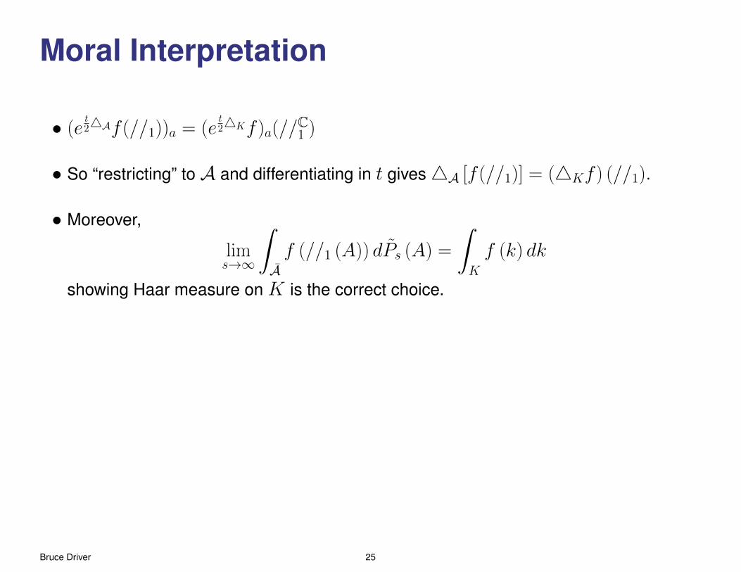
Moral Interpretation

• (et24Af (//1))a = (e

t24Kf )a(//

C1 )

• So “restricting” to A and differentiating in t gives4A [f (//1)] = (4Kf ) (//1).

• Moreover,

lims→∞

∫Af (//1 (A)) dPs (A) =

∫K

f (k) dk

showing Haar measure on K is the correct choice.

Bruce Driver 25

Corollary: Extended Hall’s Transform

Let ρs(dx) = Law(//1) and ms,t(dg) = Law(//C1 ) so that

ρs(x) =(es∆K/2δe

)(x) for x ∈ K &

ms,t(g) =(eAs,t/2δe

)(g) for g ∈ KC.

Corollary 11 (A One Parameter family of Hall’s Transforms). The map

f ∈ L2(K, ρs)→(et∆K/2f

)a∈ HL2(KC,ms,t)

is unitary. Note that ms,t is the convolution heat kernel for eAs,t/2.

This theorem interpolates between the two previous versions of Hall’s transformcorresponding to s =∞ and s = t

2.

Bruce Driver 26

Key Ingredients of the Proof 9

• Compute the action of the Segal-Bargmann transform on multiple Wiener integrals.

• Use the [Veretennikov & Krylov, 1976] formula twice to develop f (//1) and F (//C1 )into an infinite sum of multiple Wiener integrals (the Ito chaos expansion).

• Use these two items together to show St [f (//1)] = F (//C1 ).

Remark 12. See Dimock 1996, and Landsman and Wren ( ∼= 1998) for other approachesto “canonical quantization” of YM2.

Bruce Driver 27

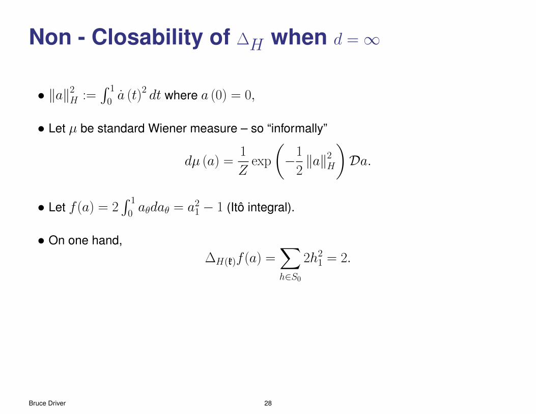
Non - Closability of ∆H when d =∞

• ‖a‖2H :=

∫ 1

0a (t)2 dt where a (0) = 0,

• Let µ be standard Wiener measure – so “informally”

dµ (a) =1

Zexp

(−1

2‖a‖2

H

)Da.

• Let f (a) = 2∫ 1

0aθdaθ = a2

1 − 1 (Ito integral).

• On one hand,∆H(k)f (a) =

∑h∈S0

2h21 = 2.

Bruce Driver 28

• On the other hand, we have f (a) = lim|P|→0 fP(a) where fP(a) is the cylinderfunction

fP(a) = 2∑si∈P

asi(asi+1 − asi)

which are all Harmonic, i.e.∆H(k)fP(a) = 0!

(Compare with the harmonic function

(x1 + x2 + · · · + xn)xn+1 on Rn+1.)

Therefore lim|P|→0 fP = f while

0 = lim|P|→0

∆H(k)fP(a) 6= ∆H(k)f = 2.

Bruce Driver 29

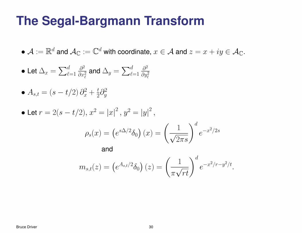
The Segal-Bargmann Transform

• A := Rd and AC := Cd with coordinate, x ∈ A and z = x + iy ∈ AC.

• Let ∆x =∑d

`=1∂2

∂x2`and ∆y =

∑d`=1

∂2

∂y2`

• As,t = (s− t/2) ∂2x + t

2∂2y

• Let r = 2(s− t/2), x2 = |x|2 , y2 = |y|2 ,

ρs(x) =(es∆/2δ0

)(x) =

(1√2πs

)d

e−x2/2s

and

ms,t(z) =(eAs,t/2δ0

)(z) =

(1

π√rt

)d

e−x2/r−y2/t.

Bruce Driver 30

Theorem 13 (Segal - Bargmann). For all s > t/2, z ∈ C and f ∈ L2(A, ps(x)dx) let

Stf := (Analytic Continuation) et∆/2f,

more explicitly,

(Stf ) (z) =

∫Af (y)pt(z − y)dy =

(et∆/2f

)a

(z).

ThenSt : L2(A, ps(x)dx)→ HL2(AC,ms,t(z)dz)

is a unitary map.

Sketch of the isometry proof

• Let ∂j := 12

(∂∂xj− i ∂∂yj

)and ∂j := 1

2

(∂∂xj

+ i ∂∂yj

)• Let f (x) be a polynomial in x ∈ A,

• Let f (z) be its analytic continuation to z ∈ AC,

• Define Ft(z) :=(e−t∆x/2f

)(z) so that f = e−

t2∆xFt = e−

t2∂

2Ft.

Bruce Driver 31

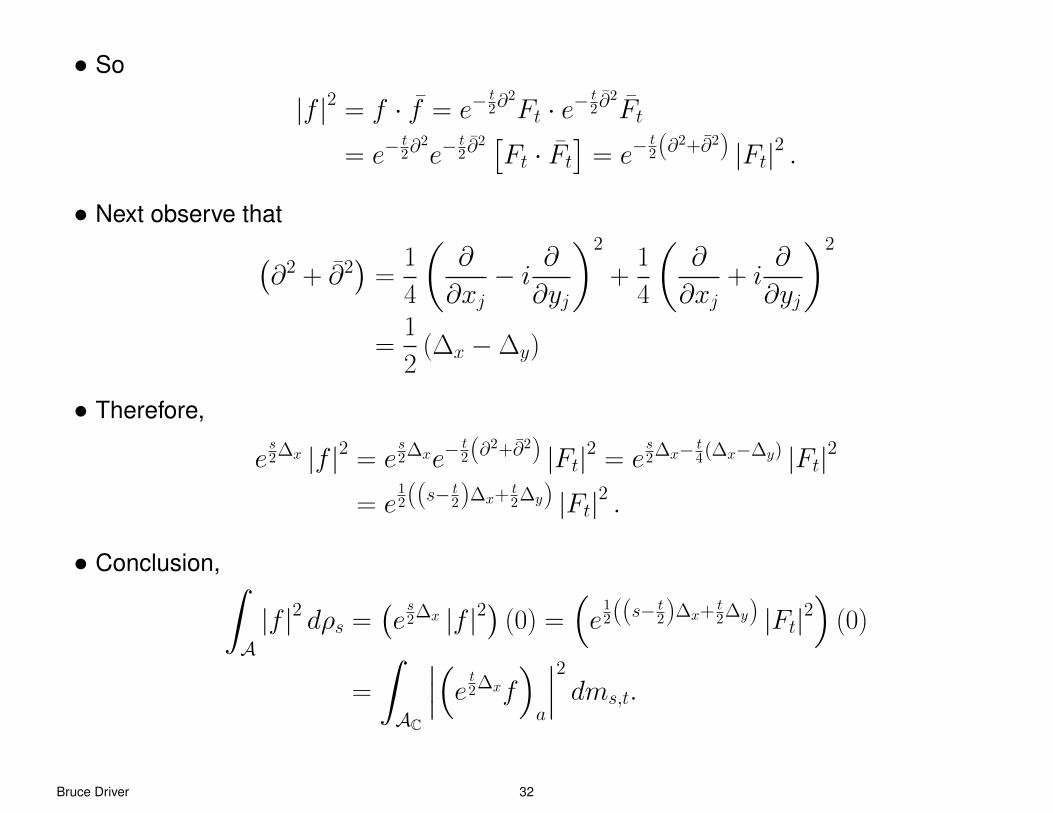
• So

|f |2 = f · f = e−t2∂

2

Ft · e−t2 ∂

2

Ft

= e−t2∂

2

e−t2 ∂

2 [Ft · Ft

]= e−

t2(∂2+∂2) |Ft|2 .

• Next observe that(∂2 + ∂2

)=

1

4

(∂

∂xj− i ∂

∂yj

)2

+1

4

(∂

∂xj+ i

∂

∂yj

)2

=1

2(∆x −∆y)

• Therefore,

es2∆x |f |2 = e

s2∆xe−

t2(∂2+∂2) |Ft|2 = e

s2∆x− t

4(∆x−∆y) |Ft|2

= e12((s−

t2)∆x+ t

2∆y) |Ft|2 .

• Conclusion,∫A|f |2 dρs =

(es2∆x |f |2

)(0) =

(e12((s−

t2)∆x+ t

2∆y) |Ft|2)

(0)

=

∫AC

∣∣∣(e t2∆xf

)a

∣∣∣2 dms,t.

Bruce Driver 32

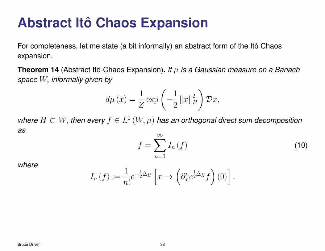
Abstract Ito Chaos Expansion

For completeness, let me state (a bit informally) an abstract form of the Ito Chaosexpansion.

Theorem 14 (Abstract Ito-Chaos Expansion). If µ is a Gaussian measure on a Banachspace W, informally given by

dµ (x) =1

Zexp

(−1

2‖x‖2

H

)Dx,

where H ⊂ W, then every f ∈ L2 (W,µ) has an orthogonal direct sum decompositionas

f =

∞∑n=0

In (f ) (10)

where

In (f ) :=1

n!e−

12∆H

[x→

(∂nxe

12∆Hf

)(0)].

Bruce Driver 33

Proof Ideas

1. f = e−12∆He

12∆Hf,

2. e12∆Hf is smooth and so(

e12∆Hf

)(x) =

∞∑n=0

1

n!

(∂nxe

12∆Hf

)(0) .

3. Combing items 1. and 2. explains Eq. (10).

4. By more elementary Taylor theorem arguments, on may show∫HIm (f ) In (f )dµ = 0 if m 6= n.

5. This is based on the identity,

E[(e−

12∆p)·(e−

12∆q)]

=

∞∑n=0

1

n!〈(Dnp) (0) , (Dnq) (0)〉(H∗)⊗n .

which is valid for any polynomials p and q.

EndBruce Driver 34

REFERENCES

References

[Bogachev, 1998] Bogachev, Vladimir I. 1998. Gaussian measures. MathematicalSurveys and Monographs, vol. 62. Providence, RI: American Mathematical Society.

[Da Prato & Zabczyk, 1992] Da Prato, Giuseppe, & Zabczyk, Jerzy. 1992. Stochasticequations in infinite dimensions. Encyclopedia of Mathematics and its Applications, vol.44. Cambridge: Cambridge University Press.

[Driver & Hall, 1999] Driver, Bruce K., & Hall, Brian C. 1999. Yang-Mills theory and theSegal-Bargmann transform. Comm. math. phys., 201(2), 249–290.

[Driver & Hall, 2000] Driver, Bruce K., & Hall, Brian C. 2000. The energy representationhas no non-zero fixed vectors. Pages 143–155 of: Stochastic processes, physics andgeometry: new interplays, II (Leipzig, 1999). CMS Conf. Proc., vol. 29. Amer. Math.Soc., Providence, RI.

[Driver et al., 2013] Driver, Bruce K., Hall, Brian C., & Kemp, Todd. 2013. The large-Nlimit of the Segal-Bargmann transform on UN . J. funct. anal., 265(11), 2585–2644.

[Hall, 1999] Hall, Brian C. 1999. A new form of the Segal-Bargmann transform for Liegroups of compact type. Canad. j. math., 51(4), 816–834.

[Hall, 2001] Hall, Brian C. 2001. Coherent states and the quantization of(1 + 1)-dimensional Yang-Mills theory. Rev. math. phys., 13(10), 1281–1305.

Bruce Driver 35

REFERENCES

[Hall, 2002] Hall, Brian C. 2002. Geometric quantization and the generalizedSegal-Bargmann transform for Lie groups of compact type. Comm. math. phys.,226(2), 233–268.

[Hall, 2003] Hall, Brian C. 2003. The Segal-Bargmann transform and the Grossergodicity theorem. Pages 99–116 of: Finite and infinite dimensional analysis in honorof Leonard Gross (New Orleans, LA, 2001). Contemp. Math., vol. 317. Amer. Math.Soc., Providence, RI.

[Kuo, 1975] Kuo, Hui Hsiung. 1975. Gaussian measures in Banach spaces. Berlin:Springer-Verlag. Lecture Notes in Mathematics, Vol. 463.

[Veretennikov & Krylov, 1976] Veretennikov, A. Ju., & Krylov, N. V. 1976. Explicit formulaefor the solutions of stochastic equations. Mat. sb. (n.s.), 100(142)(2), 266–284, 336.

Bruce Driver 36