www.elsevier.com/locate/ultras

Ultrasonics 44 (2006) e5–e15

Synthetic aperture ultrasound imaging

Jørgen Arendt Jensen *, Svetoslav Ivanov Nikolov, Kim Løkke Gammelmark,Morten Høgholm Pedersen

Center for Fast Ultrasound Imaging, Ørsted•DTU, Building 348, Technical University of Denmark, DK-2800 Lyngby, Denmark

Available online 11 August 2006

Abstract

The paper describes the use of synthetic aperture (SA) imaging in medical ultrasound. SA imaging is a radical break with today’scommercial systems, where the image is acquired sequentially one image line at a time. This puts a strict limit on the frame rate andthe possibility of acquiring a sufficient amount of data for high precision flow estimation. These constrictions can be lifted by employingSA imaging. Here data is acquired simultaneously from all directions over a number of emissions, and the full image can be reconstructedfrom this data. The paper demonstrates the many benefits of SA imaging. Due to the complete data set, it is possible to have bothdynamic transmit and receive focusing to improve contrast and resolution. It is also possible to improve penetration depth by employingcodes during ultrasound transmission. Data sets for vector flow imaging can be acquired using short imaging sequences, whereby boththe correct velocity magnitude and angle can be estimated. A number of examples of both phantom and in vivo SA images will be pre-sented measured by the experimental ultrasound scanner RASMUS to demonstrate the many benefits of SA imaging.� 2006 Elsevier B.V. All rights reserved.

Keywords: Ultrasound imaging; Synthetic aperture; Vector velocity estimation

1. Introduction

The paper gives a review of synthetic aperture (SA) tech-niques for medical ultrasound with a description of the cur-rent status and the obstacles towards obtaining real-timeSA imaging. Synthetic aperture techniques were originallyconceived for radar systems in the 1950s and were initiallyimplemented using digital computers in the late 1970s andmore advanced techniques were introduced in the late1980s [1]. There are many similarities between Radar andultrasound systems, but there are also very significant differ-ences. A SA Radar system usually employs one transmitterand receiver, and the aperture in synthesized by moving theantenna over the region of interest in an airplane or satellite.In medical ultrasound, the array has a fixed number of ele-ments and is usually stationary. The synthesizing is per-formed by acquiring data from parts of the array toreduce the amount of electronic channels. For Radar, theobject is most often in the far-field of the array, whereas

0041-624X/$ - see front matter � 2006 Elsevier B.V. All rights reserved.

doi:10.1016/j.ultras.2006.07.017

* Corresponding author. Fax: +45 45 88 01 17.E-mail address: jaj@oersted.dtu.dk (J.A. Jensen).

the object always is in the near-field of a medical ultrasoundsystem, which complicates the reconstruction. Since themedical array is stationary, it is possible to repeat measure-ments rapidly, which is not the case for a SA Radar systems.The position between the different elements is also fixed inultrasound, whereas the deviations from a straight flightpath for airplane often have to be compensated for in Radarsystems. A vital difference is also that the dynamic range ina Radar image is significantly less than the 40–80 dBdynamic range in ultrasound images.

All these factors affect the implementation of a medicalSA ultrasound system and many details have to be changedcompared to SA Radar systems to obtain a successfulimplementation. This paper will describe some of thechoices to be made to make a complete SA system thatincludes vector flow estimation.

Synthetic aperture imaging has been investigated inultrasonics since the late 1960 and early 1970 [2,3]. In the1970s and 1980s, it was primarily explored for nondestruc-tive testing (NDT) using a more or less direct implementa-tion of the SA principle, known today as monostaticsynthetic aperture imaging [4]. With the introduction of

e6 J.A. Jensen et al. / Ultrasonics 44 (2006) e5–e15

transducer arrays in the 1970s, focus was gradually directedtowards this application area to pursue real-time imple-mentations [5–7].

Until the beginning of 1990, the idea of applying the syn-thetic aperture imaging approach for medical ultrasoundimaging had only been considered occasionally [3,8]. In1992, O’Donnell and Thomas published a method intendedfor intravascular imaging based on synthetic aperture imag-ing utilizing a circular aperture [9]. To overcome the prob-lem with low SNR and impedance matching between thetransducer and receiver circuit, the single element transmis-sion was replaced by simultaneous excitation of a multi-ele-ment subaperture. Due to the circular surface of thetransducer, the subaperture generated a spherical wave withlimited angular extend at each emission, thus, permittingsynthetic aperture focusing to be applied. This was the firstdirect attempt to apply synthetic aperture imaging for med-ical ultrasound imaging. Since then, the application ofmulti-element subapertures to increase the SNR of syn-thetic aperture imaging has been investigated using phasedarray transducers by Karaman and colleagues for smallscale systems [10,11], by Lockwood and colleagues forsparse synthetic aperture systems with primary focus on3D imaging applications [12,13], and by Nikolov and col-leagues for recursive ultrasound imaging [14]. In all cases,the multi-element subaperture was used to emulate the radi-ation pattern of the single element transmission by applyingde-focusing delays in such a way that a spherical wave withlimited angular extend was produced. The definition of syn-thetic transmit aperture (STA) imaging was introduced byChiao and colleagues in [15]. This paper also consideredthe feasibility of applying spatial encoding to enable trans-mission on several elements simultaneously, while separat-ing the individual transmissions in the receiver usingaddition and subtraction of the received signals. A thirdapproach, which utilizes orthogonal Golay codes toincrease the SNR, while transmitting simultaneously onseveral elements, was also considered by Chiao and Thomasin [16].

The influence of motion in STA imaging and methodsfor compensation have been investigated in several publica-tions [17–21]. Commonly it is reported that axial motion isthe dominant factor causing image quality degradation dueto the significantly higher spatial frequency in this dimen-sion. The presented motion estimation methods are gener-ally based on time-domain cross-correlation of referencesignals to find the shift in position in the axial dimension.Since tissue motion is inherently three dimensional, it ishowever likely, that to retain the advantages of STA imag-ing, at least two dimensional (2D) motion correction tocompensate successfully for scan plane tissue motion isrequired.

2. Conventional ultrasound imaging

Conventional ultrasound images are acquired sequen-tially one image line at a time. The acquisition rate is, thus,

limited by the speed of sound c, and the maximum framerate fr for an image with Nl lines to a depth of D is

fr ¼c

2DN l

: ð1Þ

For larger depths and increasing number of lines the framerate gets progressively lower. The approximate 3-dB reso-lution of an imaging array consisting of N elements witha pitch of Dp is given by

b3 dB ¼ 0:5Di

NDp

k ¼ 0:5Di

NDp

cf0

; ð2Þ

where Di is focus depth and f0 is center frequency. Assum-ing the image to cover the full size of the array and a pitchDp = k/2 then gives a frame rate of

N l ¼NDp

b3 dB

¼ 2f0

Dic; f r ¼

Dif0

DN 2ð3Þ

for a properly sampled image. Current systems increase thenumber of active elements in the beamformer and betterengineering makes it possible to increase the transducer cen-ter frequency for the same penetration depth, which lowersthe frame rate, if the image quality has to be maintained.

For flow estimation the problem is increased, since sev-eral pulse-echo lines have to be acquired from the samedirection in order to estimate the blood velocity [22]. Often8–16 lines have to be used per estimate and this corre-spondingly lowers the frame rate. It is 6.4 Hz for a depthof 15 cm, 100 image directions and 8 lines per directionfor, e.g., scanning the heart. This is an unacceptable lowrate, and the area for estimating the velocity is often limitedin conventional systems.

A further problem in conventional imaging is the singletransmit focus, so that the imaging is only optimallyfocused at one depth. This can be overcome by makingcompound imaging using a number of transmit foci, butthe frame rate is then correspondingly decreased.

There are, thus, good reasons for developing alternativesto conventional imaging, where the frame rate and singletransmit focusing problems can be solved. One alternativeis to use synthetic aperture imaging. It will be shown thatthis can solve both the frame rate and focusing problem,but it also has several problems associated with it in termsof penetration depth, flow estimation, and implementation.The following sections will address these issues and refer tosolutions in the literature.

3. Introduction to synthetic aperture imaging

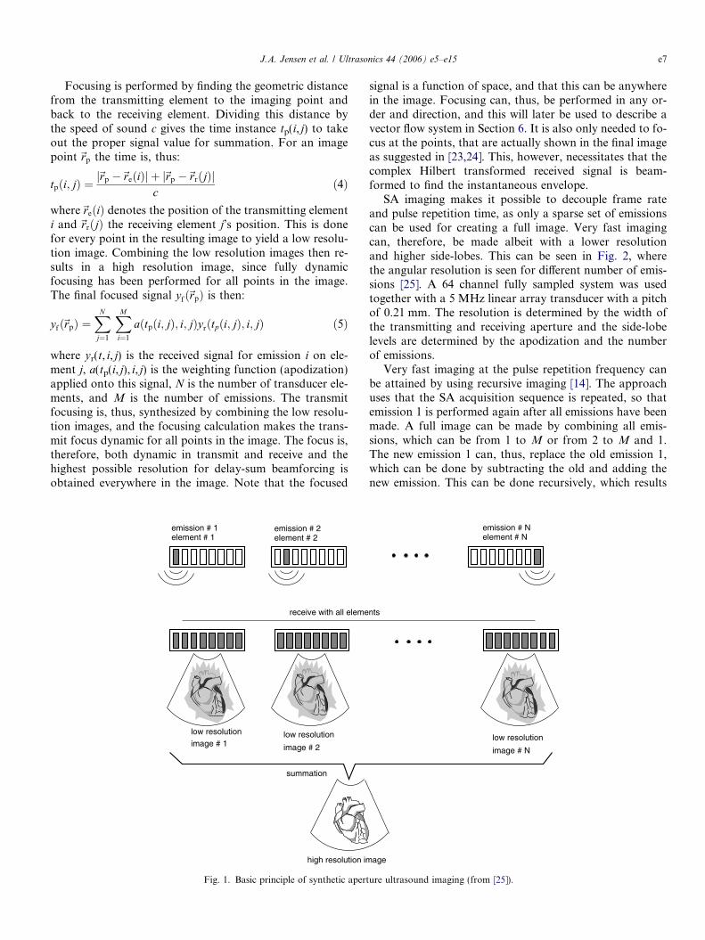
The basic method for acquiring synthetic aperture ultra-sound images is shown in Fig. 1. A single element in thetransducer aperture is used for transmitting a sphericalwave covering the full image region. The received signalsfor all or part of the elements in the aperture are sampledfor each transmission. This data can be used for makinga low resolution image, which is only focused in receivedue to the un-focused transmission.

J.A. Jensen et al. / Ultrasonics 44 (2006) e5–e15 e7

Focusing is performed by finding the geometric distancefrom the transmitting element to the imaging point andback to the receiving element. Dividing this distance bythe speed of sound c gives the time instance tp(i, j) to takeout the proper signal value for summation. For an imagepoint~rp the time is, thus:

tpði; jÞ ¼j~rp �~reðiÞj þ j~rp �~rrðjÞj

cð4Þ

where~reðiÞ denotes the position of the transmitting elementi and ~rrðjÞ the receiving element j’s position. This is donefor every point in the resulting image to yield a low resolu-tion image. Combining the low resolution images then re-sults in a high resolution image, since fully dynamicfocusing has been performed for all points in the image.The final focused signal yfð~rpÞ is then:

yfð~rpÞ ¼XN

j¼1

XM

i¼1

aðtpði; jÞ; i; jÞyrðtpði; jÞ; i; jÞ ð5Þ

where yr(t, i, j) is the received signal for emission i on ele-ment j, a(tp(i, j), i, j) is the weighting function (apodization)applied onto this signal, N is the number of transducer ele-ments, and M is the number of emissions. The transmitfocusing is, thus, synthesized by combining the low resolu-tion images, and the focusing calculation makes the trans-mit focus dynamic for all points in the image. The focus is,therefore, both dynamic in transmit and receive and thehighest possible resolution for delay-sum beamforcing isobtained everywhere in the image. Note that the focused

element # 1 element # 2 emission # 2 emission # 1

receive with all eleme

low resolution

image # 2

low resolution image # 1

summation

high resolution im

Fig. 1. Basic principle of synthetic apert

signal is a function of space, and that this can be anywherein the image. Focusing can, thus, be performed in any or-der and direction, and this will later be used to describe avector flow system in Section 6. It is also only needed to fo-cus at the points, that are actually shown in the final imageas suggested in [23,24]. This, however, necessitates that thecomplex Hilbert transformed received signal is beam-formed to find the instantaneous envelope.

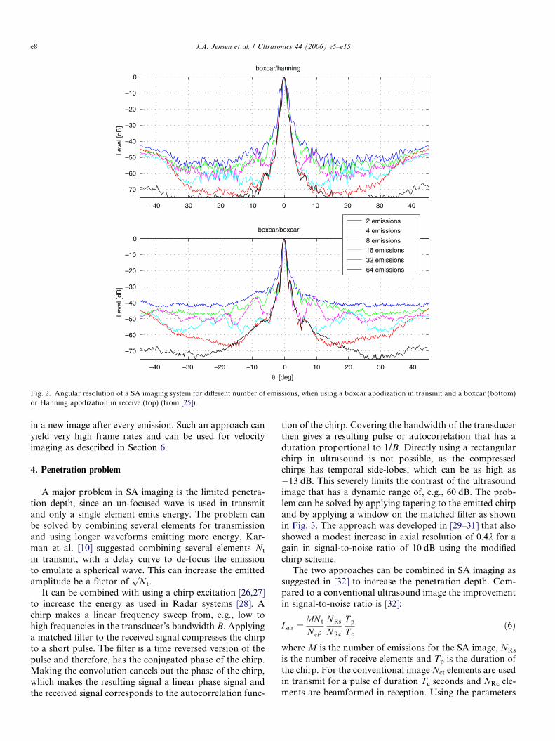
SA imaging makes it possible to decouple frame rateand pulse repetition time, as only a sparse set of emissionscan be used for creating a full image. Very fast imagingcan, therefore, be made albeit with a lower resolutionand higher side-lobes. This can be seen in Fig. 2, wherethe angular resolution is seen for different number of emis-sions [25]. A 64 channel fully sampled system was usedtogether with a 5 MHz linear array transducer with a pitchof 0.21 mm. The resolution is determined by the width ofthe transmitting and receiving aperture and the side-lobelevels are determined by the apodization and the numberof emissions.

Very fast imaging at the pulse repetition frequency canbe attained by using recursive imaging [14]. The approachuses that the SA acquisition sequence is repeated, so thatemission 1 is performed again after all emissions have beenmade. A full image can be made by combining all emis-sions, which can be from 1 to M or from 2 to M and 1.The new emission 1 can, thus, replace the old emission 1,which can be done by subtracting the old and adding thenew emission. This can be done recursively, which results

emission # N element # N

nts

low resolution

image # N

age

ure ultrasound imaging (from [25]).

–40 –30 –20 –10 0 10 20 30 40

–70

–60

–50

–40

–30

–20

–10

0

Leve

l [dB

]

–70

–60

–50

–40

–30

–20

–10

0

Leve

l [dB

]

boxcar/hanning

–40 –30 –20 –10 0 10 20 30 40

boxcar/boxcar

θ [deg]

2 emissions

4 emissions

8 emissions

16 emissions

32 emissions

64 emissions

Fig. 2. Angular resolution of a SA imaging system for different number of emissions, when using a boxcar apodization in transmit and a boxcar (bottom)or Hanning apodization in receive (top) (from [25]).

e8 J.A. Jensen et al. / Ultrasonics 44 (2006) e5–e15

in a new image after every emission. Such an approach canyield very high frame rates and can be used for velocityimaging as described in Section 6.

4. Penetration problem

A major problem in SA imaging is the limited penetra-tion depth, since an un-focused wave is used in transmitand only a single element emits energy. The problem canbe solved by combining several elements for transmissionand using longer waveforms emitting more energy. Kar-man et al. [10] suggested combining several elements Nt

in transmit, with a delay curve to de-focus the emissionto emulate a spherical wave. This can increase the emittedamplitude be a factor of

ffiffiffiffiffiN t

p.

It can be combined with using a chirp excitation [26,27]to increase the energy as used in Radar systems [28]. Achirp makes a linear frequency sweep from, e.g., low tohigh frequencies in the transducer’s bandwidth B. Applyinga matched filter to the received signal compresses the chirpto a short pulse. The filter is a time reversed version of thepulse and therefore, has the conjugated phase of the chirp.Making the convolution cancels out the phase of the chirp,which makes the resulting signal a linear phase signal andthe received signal corresponds to the autocorrelation func-

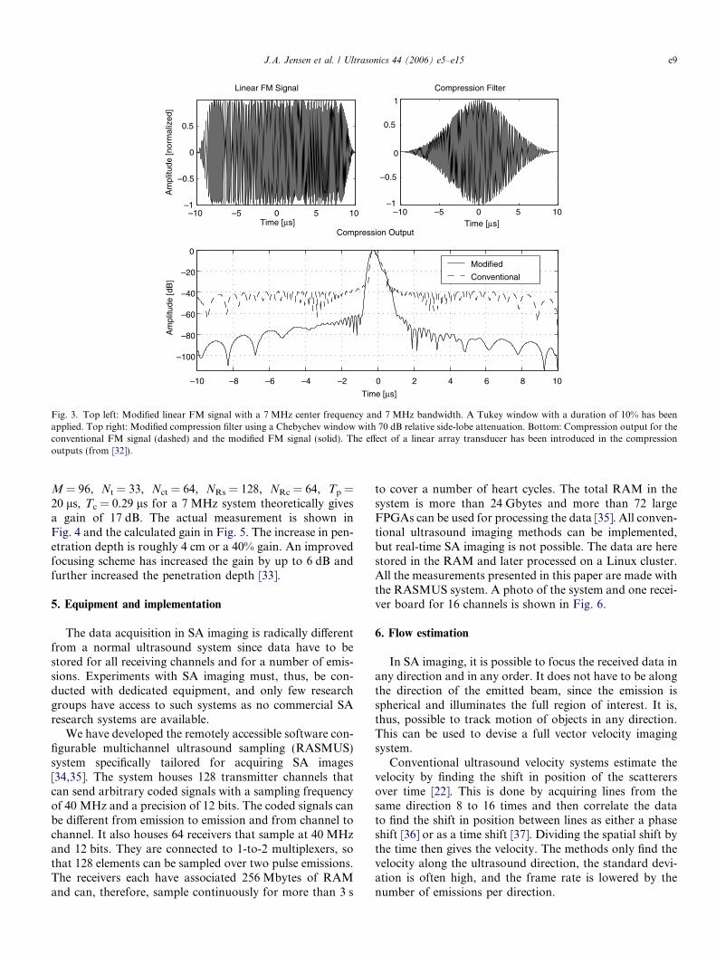
tion of the chirp. Covering the bandwidth of the transducerthen gives a resulting pulse or autocorrelation that has aduration proportional to 1/B. Directly using a rectangularchirp in ultrasound is not possible, as the compressedchirps has temporal side-lobes, which can be as high as�13 dB. This severely limits the contrast of the ultrasoundimage that has a dynamic range of, e.g., 60 dB. The prob-lem can be solved by applying tapering to the emitted chirpand by applying a window on the matched filter as shownin Fig. 3. The approach was developed in [29–31] that alsoshowed a modest increase in axial resolution of 0.4k for again in signal-to-noise ratio of 10 dB using the modifiedchirp scheme.

The two approaches can be combined in SA imaging assuggested in [32] to increase the penetration depth. Com-pared to a conventional ultrasound image the improvementin signal-to-noise ratio is [32]:

I snr ¼MN t

N ct2

NRs

NRc

T p

T c

ð6Þ

where M is the number of emissions for the SA image, NRs

is the number of receive elements and Tp is the duration ofthe chirp. For the conventional image Nct elements are usedin transmit for a pulse of duration Tc seconds and NRc ele-ments are beamformed in reception. Using the parameters

–10 –5 0 5 10–1

–0.5

0

0.5

Time [μs]

Am

plitu

de [n

orm

aliz

ed]

Linear FM Signal

–10 –5 0 5 10–1

–0.5

0

0.5

1

Time [μs]

Compression Filter

–10 –8 –6 –4 –2 0 2 4 6 8 10

–100

–80

–60

–40

–20

0

Time [μs]

Am

plitu

de [d

B]

Compression Output

Modified

Conventional

Fig. 3. Top left: Modified linear FM signal with a 7 MHz center frequency and 7 MHz bandwidth. A Tukey window with a duration of 10% has beenapplied. Top right: Modified compression filter using a Chebychev window with 70 dB relative side-lobe attenuation. Bottom: Compression output for theconventional FM signal (dashed) and the modified FM signal (solid). The effect of a linear array transducer has been introduced in the compressionoutputs (from [32]).

J.A. Jensen et al. / Ultrasonics 44 (2006) e5–e15 e9

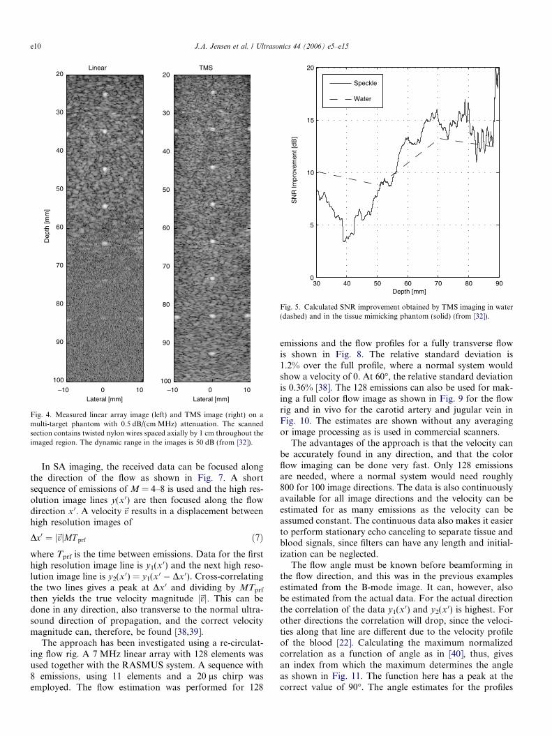
M = 96, Nt = 33, Nct = 64, NRs = 128, NRc = 64, Tp =20 ls, Tc = 0.29 ls for a 7 MHz system theoretically givesa gain of 17 dB. The actual measurement is shown inFig. 4 and the calculated gain in Fig. 5. The increase in pen-etration depth is roughly 4 cm or a 40% gain. An improvedfocusing scheme has increased the gain by up to 6 dB andfurther increased the penetration depth [33].

5. Equipment and implementation

The data acquisition in SA imaging is radically differentfrom a normal ultrasound system since data have to bestored for all receiving channels and for a number of emis-sions. Experiments with SA imaging must, thus, be con-ducted with dedicated equipment, and only few researchgroups have access to such systems as no commercial SAresearch systems are available.

We have developed the remotely accessible software con-figurable multichannel ultrasound sampling (RASMUS)system specifically tailored for acquiring SA images[34,35]. The system houses 128 transmitter channels thatcan send arbitrary coded signals with a sampling frequencyof 40 MHz and a precision of 12 bits. The coded signals canbe different from emission to emission and from channel tochannel. It also houses 64 receivers that sample at 40 MHzand 12 bits. They are connected to 1-to-2 multiplexers, sothat 128 elements can be sampled over two pulse emissions.The receivers each have associated 256 Mbytes of RAMand can, therefore, sample continuously for more than 3 s

to cover a number of heart cycles. The total RAM in thesystem is more than 24 Gbytes and more than 72 largeFPGAs can be used for processing the data [35]. All conven-tional ultrasound imaging methods can be implemented,but real-time SA imaging is not possible. The data are herestored in the RAM and later processed on a Linux cluster.All the measurements presented in this paper are made withthe RASMUS system. A photo of the system and one recei-ver board for 16 channels is shown in Fig. 6.

6. Flow estimation

In SA imaging, it is possible to focus the received data inany direction and in any order. It does not have to be alongthe direction of the emitted beam, since the emission isspherical and illuminates the full region of interest. It is,thus, possible to track motion of objects in any direction.This can be used to devise a full vector velocity imagingsystem.

Conventional ultrasound velocity systems estimate thevelocity by finding the shift in position of the scatterersover time [22]. This is done by acquiring lines from thesame direction 8 to 16 times and then correlate the datato find the shift in position between lines as either a phaseshift [36] or as a time shift [37]. Dividing the spatial shift bythe time then gives the velocity. The methods only find thevelocity along the ultrasound direction, the standard devi-ation is often high, and the frame rate is lowered by thenumber of emissions per direction.

30 40 50 60 70 80 900

5

10

15

20

SN

R Im

prov

emen

t [dB

]Depth [mm]

Speckle

Water

Fig. 5. Calculated SNR improvement obtained by TMS imaging in water(dashed) and in the tissue mimicking phantom (solid) (from [32]).

Dep

th [m

m]

Lateral [mm]

Linear

–10 0 10

20

30

40

50

60

70

80

90

100

TMS

Lateral [mm]–10 0 10

20

30

40

50

60

70

80

90

100

Fig. 4. Measured linear array image (left) and TMS image (right) on amulti-target phantom with 0.5 dB/(cm MHz) attenuation. The scannedsection contains twisted nylon wires spaced axially by 1 cm throughout theimaged region. The dynamic range in the images is 50 dB (from [32]).

e10 J.A. Jensen et al. / Ultrasonics 44 (2006) e5–e15

In SA imaging, the received data can be focused alongthe direction of the flow as shown in Fig. 7. A shortsequence of emissions of M = 4–8 is used and the high res-olution image lines y(x 0) are then focused along the flowdirection x 0. A velocity~v results in a displacement betweenhigh resolution images of

Dx0 ¼ j~vjMT prf ð7Þwhere Tprf is the time between emissions. Data for the firsthigh resolution image line is y1(x 0) and the next high reso-lution image line is y2(x 0) = y1(x 0 � Dx 0). Cross-correlatingthe two lines gives a peak at Dx 0 and dividing by MTprf

then yields the true velocity magnitude j~vj. This can bedone in any direction, also transverse to the normal ultra-sound direction of propagation, and the correct velocitymagnitude can, therefore, be found [38,39].

The approach has been investigated using a re-circulat-ing flow rig. A 7 MHz linear array with 128 elements wasused together with the RASMUS system. A sequence with8 emissions, using 11 elements and a 20 ls chirp wasemployed. The flow estimation was performed for 128

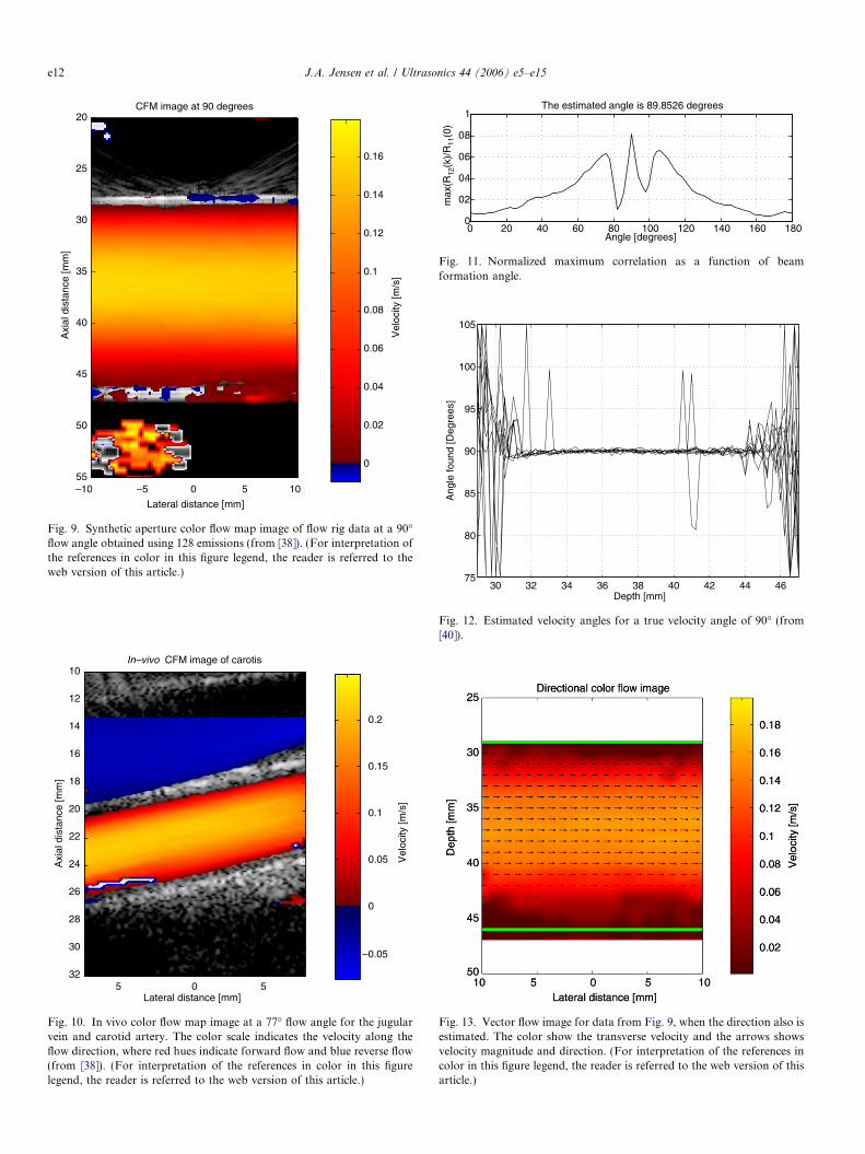
emissions and the flow profiles for a fully transverse flowis shown in Fig. 8. The relative standard deviation is1.2% over the full profile, where a normal system wouldshow a velocity of 0. At 60�, the relative standard deviationis 0.36% [38]. The 128 emissions can also be used for mak-ing a full color flow image as shown in Fig. 9 for the flowrig and in vivo for the carotid artery and jugular vein inFig. 10. The estimates are shown without any averagingor image processing as is used in commercial scanners.

The advantages of the approach is that the velocity canbe accurately found in any direction, and that the colorflow imaging can be done very fast. Only 128 emissionsare needed, where a normal system would need roughly800 for 100 image directions. The data is also continuouslyavailable for all image directions and the velocity can beestimated for as many emissions as the velocity can beassumed constant. The continuous data also makes it easierto perform stationary echo canceling to separate tissue andblood signals, since filters can have any length and initial-ization can be neglected.

The flow angle must be known before beamforming inthe flow direction, and this was in the previous examplesestimated from the B-mode image. It can, however, alsobe estimated from the actual data. For the actual directionthe correlation of the data y1(x 0) and y2(x 0) is highest. Forother directions the correlation will drop, since the veloci-ties along that line are different due to the velocity profileof the blood [22]. Calculating the maximum normalizedcorrelation as a function of angle as in [40], thus, givesan index from which the maximum determines the angleas shown in Fig. 11. The function here has a peak at thecorrect value of 90�. The angle estimates for the profiles

Fig. 6. Photos of the RASMUS scanner (left) with one of the 8 channel receiver boards. The digital part of the system is shown with the 64 receivers in thetop cabinet, the 128 transmitters in the middle, and the analog power supplies on the bottom. The analog front-end and transducer plug are at the otherside of the 19 in. racks. (from [35]).

z

x

Blood vessel

Beams

along

the vessel

Velocity

profile

θ

Fig. 7. Beamforming is made along the laminar flow (from [38]).

30 35 40 45 50

0

0.1

0.2

Depth [mm]

Vel

ocity

[m/s

]

Measured velocity profiles at 90 deg., 16 sequences of 8 emissions

30 35 40 45 50

0

0.1

0.2

Depth [mm]

Vel

ocity

[m/s

]

Mean +/ 3 std. for measured profile

Fig. 8. Estimated profiles from the flow rig at a 90� flow angle. The topgraph shows 20 independent profiles estimated and the bottom graphshows the mean profile (solid line) ± 3 standard deviations (dashed lines).From [38].

J.A. Jensen et al. / Ultrasonics 44 (2006) e5–e15 e11

shown in Fig. 9 are shown in Fig. 12. The mean value is90.0003� and the standard deviation is 1.32� [40]. Theresulting color flow image with arrows indicating directionand magnitude is shown in Fig. 13.

7. Motion compensation

The accurate velocity estimation can also be used forcompensating for tissue motion during the SA acquisi-

tion process. High quality SA images will often takeup to 100 emissions and high tissue velocities willdegrade the image quality since the individual low reso-lution images are not summed in phase. The B-modesequence can then be inter-spaced with a flow sequenceand the tissue velocity can be estimated from this data.Knowing the velocity is then used for correcting theposition of the low resolution images that then can besummed in phase. This was suggested in [32,25], where

Lateral distance [mm]

Axi

al d

ista

nce

[mm

]

In–vivo CFM image of carotis

5 0 5

10

12

14

16

18

20

22

24

26

28

30

32

Vel

ocity

[m/s

]

–0.05

0

0.05

0.1

0.15

0.2

Fig. 10. In vivo color flow map image at a 77� flow angle for the jugularvein and carotid artery. The color scale indicates the velocity along theflow direction, where red hues indicate forward flow and blue reverse flow(from [38]). (For interpretation of the references in color in this figurelegend, the reader is referred to the web version of this article.)

0 20 40 60 80 100 120 140 160 1800

0.2

0.4

0.6

0.8

1

Angle [degrees]

max

(R12

(k)/

R11

(0)

The estimated angle is 89.8526 degrees

Fig. 11. Normalized maximum correlation as a function of beamformation angle.

30 32 34 36 38 40 42 44 4675

80

85

90

95

100

105

Depth [mm]

Ang

le fo

und

[Deg

rees

]

Fig. 12. Estimated velocity angles for a true velocity angle of 90� (from[40]).

Fig. 13. Vector flow image for data from Fig. 9, when the direction also isestimated. The color show the transverse velocity and the arrows showsvelocity magnitude and direction. (For interpretation of the references incolor in this figure legend, the reader is referred to the web version of thisarticle.)

Lateral distance [mm]

Axi

al d

ista

nce

[mm

]

CFM image at 90 degrees

–10 –5 0 5 10

20

25

30

35

40

45

50

55

Vel

ocity

[m/s

]

0

0.02

0.04

0.06

0.08

0.1

0.12

0.14

0.16

Fig. 9. Synthetic aperture color flow map image of flow rig data at a 90�flow angle obtained using 128 emissions (from [38]). (For interpretation ofthe references in color in this figure legend, the reader is referred to theweb version of this article.)

e12 J.A. Jensen et al. / Ultrasonics 44 (2006) e5–e15

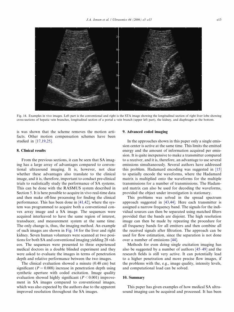
Fig. 14. Examples in vivo images. Left part is the conventional and right is the STA image showing the longitudinal section of right liver lobe showingcross-sections of hepatic vein branches, longitudinal section of a portal a vein branch (upper left part), the kidney, and diaphragm at the bottom.

J.A. Jensen et al. / Ultrasonics 44 (2006) e5–e15 e13

is was shown that the scheme removes the motion arti-facts. Other motion compensation schemes have beenstudied in [17,19,25].

8. Clinical results

From the previous sections, it can be seen that SA imag-ing has a large array of advantages compared to conven-tional ultrasound imaging. It is, however, not clearwhether these advantages also translate to the clinicalimage, and it is, therefore, important to conduct pre-clinicaltrials to realistically study the performance of SA systems.This can be done with the RASMUS system described inSection 5. It is here possible to acquire in vivo real-time dataand then make off-line processing for finding the clinicalperformance. This has been done in [41,42], where the sys-tem was programmed to acquire both a conventional con-vex array image and a SA image. The sequences wereacquired interleaved to have the same region of interest,transducer, and measurement system at the same time.The only change is, thus, the imaging method. An exampleof such images are shown in Fig. 14 for the liver and rightkidney. Seven human volunteers were scanned at two posi-tions for both SA and conventional imaging yielding 28 vid-eos. The sequences were presented to three experiencedmedical doctors in a double blinded experiment and theywere asked to evaluate the images in terms of penetrationdepth and relative performance between the two images.

The clinical evaluation showed a minute (0.48 cm) butsignificant (P = 0.008) increase in penetration depth usingsynthetic aperture with coded excitation. Image qualityevaluation showed highly significant (P < 0.001) improve-ment in SA images compared to conventional images,which was also expected by the authors due to the apparentimproved resolution throughout the SA images.

9. Advanced coded imaging

In the approaches shown in this paper only a single emis-sion center is active at the same time. This limits the emittedenergy and the amount of information acquired per emis-sion. It is quite inexpensive to make a transmitter comparedto a receiver, and it is, therefore, an advantage to use severalemissions simultaneously. Several authors have addressedthis problem. Hadamard encoding was suggested in [15]to spatially encode the waveforms, where the Hadamardmatrix is multiplied onto the waveforms for the multipletransmissions for a number of transmissions. The Hadam-ard matrix can also be used for decoding the waveforms,provided the object under investigation is stationary.

This problems was solved in the spread spectrumapproach suggested in [43,44]. Here each transmitter isassigned a narrow frequency band. The signals for the indi-vidual sources can then be separated using matched filtersprovided that the bands are disjoint. The high resolutionimage can then be made by repeating the procedure forall frequency bands for all emitters and then combine allthe received signals after filtration. The approach can beused for flow estimation, since the separation is not doneover a number of emissions [44].

Methods for even doing single excitation imaging hasalso be suggested by a number of authors [45–49] and theresearch fields is still very active. It can potentially leadto a higher penetration and more precise flow images, ifthe problems with the, e.g., image quality, intensity levels,and computational load can be solved.

10. Summary

This paper has given examples of how medical SA ultra-sound imaging can be acquired and processed. It has been

e14 J.A. Jensen et al. / Ultrasonics 44 (2006) e5–e15

shown that problems with penetration depth, flow, andmotion can be solved, and that high quality in vivo SAimages can be acquired. It has been demonstrated inpre-clinical studies on human volunteers that the SA imageresolution and penetration depth are larger than for con-ventional ultrasound images. Further, the data can be usedfor vectorial velocity estimation, where both direction andmagnitude of the flow vectors can be determined in anydirection with a relative standard deviation of a few percentmaking it possible to construct quantitative SA vector flowsystems.

References

[1] M. Soumekh, Synthetic Aperture Radar. Signal Processing withMATLAB Algorithms, John Wiley & Sons, Inc., New York, 1999.

[2] J.J. Flaherty, K.R. Erikson, V.M. Lund. Synthetic aperture ultra-sound imaging systems, United States Patent, US 3,548,642, 1967.

[3] C.B. Burckhardt, P-A. Grandchamp, H. Hoffmann, An experimental2 MHz synthetic aperture sonar system intended for medical use,IEEE Trans. Son. Ultrason. 21 (1) (1974) 1–6.

[4] J.T. Ylitalo, H. Ermert, Ultrasound synthetic aperture imaging:monostatic approach, IEEE Trans. Ultrason. Ferroelec. Freq. Contr.41 (1994) 333–339.

[5] P.D. Corl, P.M. Grant, G.S. Kino, A digital synthetic focus acousticimaging system for NDE, in: Proceedings of the IEEE UltrasonicSymposium, 1978, pp. 263–268.

[6] G.S. Kino, D. Corl, S. Bennett, K. Peterson, Real time syntheticaperture imaging system, in: Proceedings of the IEEE UltrasonicSymposium, 1980, pp. 722–731.

[7] D.K. Peterson, G.S. Kino, Real-time digital image reconstruction: adescription of imaging hardware and an analysis of quantizationerrors, IEEE Trans. Son. Ultrason. 31 (1984) 337–351.

[8] K. Nagai, A new synthetic-aperture focusing method for ultrasonic B-scan imaging by the fourier transform, IEEE Trans. Son. Ultrason.SU-32 (4) (1985) 531–536.

[9] M. O’Donnell, L.J. Thomas, Efficient synthetic aperture imagingfrom a circular aperture with possible application to catheter-basedimaging, IEEE Trans. Ultrason. Ferroelec. Freq. Contr. 39 (1992)366–380.

[10] M. Karaman, P.C. Li, M. O’Donnell, Synthetic aperture imaging forsmall scale systems, IEEE Trans. Ultrason. Ferroelec. Freq. Contr. 42(1995) 429–442.

[11] M. Karaman, M. O’Donnell, Subaperture processing for ultrasonicimaging, IEEE Trans. Ultrason. Ferroelec. Freq. Contr. 45 (1998)126–135.

[12] G.R. Lockwood, F.S. Foster, Design of sparse array imaging systems,in: Proceedings of the IEEE Ultrasonic Symposium, 1995 pp. 1237–1243.

[13] G.R. Lockwood, J.R. Talman, S.S. Brunke, Real-time 3-D ultra-sound imaging using sparse synthetic aperture beamforming, IEEETrans. Ultrason. Ferroelec. Freq. Contr. 45 (1998) 980–988.

[14] S.I. Nikolov, K. Gammelmark, J.A. Jensen, Recursive ultrasoundimaging, in: Proceedings of the IEEE Ultrasonic Symposium, vol. 2,1999, pp. 1621–1625.

[15] R.Y. Chiao, L.J. Thomas, S.D. Silverstein, Sparse array imaging withspatially-encoded transmits, in: Proceedings of the IEEE UltrasonicSymposium, 1997, pp. 1679–1682.

[16] R.Y. Chiao, L.J. Thomas, Synthetic transmit aperture using orthog-onal golay coded excitation, in: Proceedings of the IEEE UltrasonicSymposium, 2000, pp. 1469–1472.

[17] G.E. Trahey, L.F. Nock, Synthetic receive aperture imaging withphase correction for motion and for tissue inhomogenities – part II:effects of and correction for motion, IEEE Trans. Ultrason. Ferroelec.Freq. Contr. 39 (1992) 496–501.

[18] H.S�. Bilge, M. Karaman, M. O’Donnell, Motion estimation usingcommon spatial frequencies in synthetic aperture imaging, in:Proceedings of the IEEE Ultrasonic Symposium, 1996, pp. 1551–1554.

[19] M. Karaman, H.S�. Bilge, M. O’Donnell, Adaptive multi-elementsynthetic aperture imaging with motion and phase aberation correc-tion, IEEE Trans. Ultrason. Ferroelec. Freq. Contr. 42 (1998) 1077–1087.

[20] C.R. Hazard, G.R. Lockwood, Effects of motion artifacts on asynthetic aperture beamformer for real-time 3D ultrasound, in:Proceedings of the IEEE Ultrasonic Symposium, 1999, pp. 1221–1224.

[21] J.S. Jeong, J.S. Hwang, M.H. Bae, T.K. Song, Effects and limitationsof motion compensation in synthetic aperture techniques, in:Proceedings of the IEEE Ultrasonic Symposium, 2000, pp. 1759–1762.

[22] J.A. Jensen, Estimation of Blood Velocities Using Ultrasound: ASignal Processing Approach, Cambridge University Press, New York,1996.

[23] M. Karaman, A. Atalar, H. Koymen, VLSI circuits for adaptivedigital beamforming in ultrasound imaging, IEEE Trans. Med. Imag.12 (1993) 711–720.

[24] B.G. Tomov, J.A. Jensen, Compact implementation of dynamicreceive apodization in ultrasound scanners. in: Proceedings of theSPIE – Medical Imaging, 2004, pp. 260–271.

[25] S.I. Nikolov, Synthetic aperture tissue and flow ultrasound imaging,PhD Thesis, Ørsted. DTU, Technical University of Denmark, 2800,Lyngby, Denmark, 2001.

[26] Y. Takeuchi, An investigation of a spread energy method for medicalultrasound systems – part one: theory and investigations, Ultrasonics(1979) pp. 175–182.

[27] M. O’Donnell, Coded excitation system for improving the penetra-tion of real-time phased-array imaging systems, IEEE Trans. Ultra-son. Ferroelec. Freq. Contr. 39 (1992) 341–351.

[28] M.I. Skolnik, Introduction to Radar Systems, McGraw-Hill, NewYork, 1980.

[29] T. Misaridis, Ultrasound imaging using coded signals, PhD Thesis,Ørsted. DTU, Technical University of Denmark, Lyngby, Denmark,2001.

[30] T.X. Misaridis, K. Gammelmark, C.H. Jørgensen, N. Lindberg, A.H.Thomsen, M.H. Pedersen, J.A. Jensen, Potential of coded excitationin medical ultrasound imaging, Ultrasonics 38 (2000) 183–189.

[31] T. Misaridis, J.A. Jensen, Use of modulated excitation signals inultrasound. Part I: basic concepts and expected benefits, IEEE Trans.Ultrason. Ferroelec. Freq. Contr. (2005) 192–207.

[32] K.L. Gammelmark, J.A. Jensen, Multielement synthetic transmitaperture imaging using temporal encoding, IEEE Trans. Med. Imag.22 (4) (2003) 552–563.

[33] K. Gammelmark, Improving the Image Quality of Synthetic TransmitAperture Ultrasound Images, PhD Thesis, Ørsted. DTU, TechnicalUniversity of Denmark, 2800, Lyngby, Denmark, 2004.

[34] J.A. Jensen, O. Holm, L.J. Jensen, H. Bendsen, H.M. Pedersen, K.Salomonsen, J. Hansen, S. Nikolov, Experimental ultrasound systemfor real-time synthetic imaging. in: Proceedings of the IEEE Ultra-sonic Symposium, vol. 2, 1999, pp. 1595–1599.

[35] J.A. Jensen, O. Holm, L.J. Jensen, H. Bendsen, S.I. Nikolov, B.G.Tomov, P. Munk, M. Hansen, K. Salomonsen, J. Hansen, K.Gormsen, H.M. Pedersen, K.L. Gammelmark, Ultrasound researchscanner for real-time synthetic aperture image acquisition, IEEETrans. Ultrason. Ferroelec. Freq. Contr. 52 (5) (2005).

[36] C. Kasai, K. Namekawa, A. Koyano, R. Omoto, Real-time two-dimensional blood flow imaging using an autocorrelation technique,IEEE Trans. Son. Ultrason. 32 (1985) 458–463.

[37] O. Bonnefous, P. Pesque, Time domain formulation of pulse-Dopplerultrasound and blood velocity estimation by cross correlation,Ultrason. Imag. 8 (1986) 73–85.

[38] J.A. Jensen, S.I. Nikolov, Directional synthetic aperture flow imag-ing, IEEE Trans. Ultrason. Ferroelec. Freq. Contr. (2004) 1107–1118.

J.A. Jensen et al. / Ultrasonics 44 (2006) e5–e15 e15

[39] J.A. Jensen, S.I. Nikolov, Transverse flow imaging using syntheticaperture directional beamforming, in: Proceedings of the IEEEUltrasonic Symposium, 2002, pp. 1488–1492.

[40] J.A. Jensen, Velocity vector estimation in synthetic aperture flow andB-mode imaging, in: IEEE International Symposium on BiomedicalImaging from Nano to Macro, 2004, pp. 32–35.

[41] M.H. Pedersen, K.L. Gammelmark, J.A. Jensen, Preliminary in vivoevaluationofconvexarraysyntheticapertureimaging, in:Proceedingsofthe SPIE – Progress in Biomedical Optics and Imaging, 2004, pp. 33–43.

[42] M.H. Pedersen, K.L. Gammelmark, J.A. Jensen, In vivo evaluationof convex array synthetic aperture imaging, Ultrasound Med. Biol.,accepted for publication.

[43] F. Gran, J.A. Jensen, Multi element synthetic aperture transmissionusing a frequency division approach, in: Proceedings of the IEEEUltrasonic Symposium, 2003, pp. 1942–1946.

[44] F. Gran, J.A. Jensen, Spatio-temporal encoding using narrow-bandlinearly frequency modulated signals in synthetic aperture ultrasoundimaging, in: Proceedings of the SPIE – Progress in Biomedical Optics

and Imaging, Ultrasonic Imaging and Signal Processing, vol. 5750,2005, pp. 405–416.

[45] J. Shen, E.S. Ebbini, A new coded-excitation ultrasound imagingsystem-part 1: basic principles, IEEE Trans. Ultrason. Ferroelec.Freq. Contr. 43 (1) (1996) 131–140.

[46] J. Shen, E.S. Ebbini, A new coded-excitation ultrasound imagingsystem-part 2: operator design, IEEE Trans. Ultrason. Ferroelec.Freq. Contr. 43 (1) (1996) 141–148.

[47] F. Gran, J.A. Jensen, A. Jakobsson, A code division technique formultiple element synthetic aperture transmission, in: Proceedings ofthe SPIE – Progress in Biomedical Optics and Imaging, vol. 5373,2004, pp. 300–306.

[48] T. Misaridis, P. Munk, J.A. Jensen, Parallel multi-focusing usingplane wave decomposition, in: Proceedings of the IEEE UltrasonicSymposium vol. 2, 2003, pp. 1565–1568.

[49] T. Misaridis, J.A. Jensen, Use of modulated excitation signals inultrasound. Part III: high frame rate imaging, IEEE Trans. Ultrason.Ferroelec. Freq. Contr. (2005) 220–230.