synthesis 2 introduction sound synthesis and manipulation · parametrization that are suitable for...
TRANSCRIPT
Synthesis 1 SGN-14006 / A.K.
Sound synthesis and manipulation Sources: -Tolonen, Välimäki, Karjalainen. (1998). ”Evaluation of modern sound synthesis
methods”. Report no. 48, Helsinki University of Technology (Available on-line) -Roads. (1996). ”Computer music tutorial”. MIT Press. -Tuomas Virtanen.(2001).”Audio signal modeling with sinusoids and noise”. MSc thesis, TUT. -Zölzer (ed.) (2002) DAFX – Digital Audio Effects. John Wiley & Sons.
Contents ! Introduction ! FM synthesis ! Sampling synthesis ! Phase vocoder ! Time stretching and pitch shifting ! Sinusoids-plus-noise spectral model
Synthesis 2 SGN-14006 / A.K. Introduction
! In this lecture, we consider some audio representations and parametrization that are suitable for sound synthesis and manipulation – We can cover only a few widely-used representations – not all
! Sound synthesis – The goal is to produce sounds that are musically interesting and (if
required) resembre a real instrument – Sounds have to be produced in real time – Intuitive control of the synthesized sound is important: interaction of the
player makes the sound lively ! Audio effects include for example
– Dynamic level control (discussed on a separate lecture) – Equalization (boosting or cutting certain frequencies = filtering) – Time stretching and pitch shifting – Adding reverberation (in its simplest form, simply filtering the ”dry” sound
with the impulse response of the target reverberant room) – Effects applied on musical sounds: flanger, chorus, phaser, wah-wah
Synthesis 3 SGN-14006 / A.K. 1 FM synthesis
! Frequency modulation (FM) has been used in telecommunications, for example in broadcast radio, already for more than half a century
! In late 1960s, John Chowning proposed to apply FM-synthesis for sound production – Idea: complex spectra can be synthesized with only a few voltage-
controlled oscillators ! In 1983 Yamaha released its DX7 synthesizer
– Great commercial success: an instrument that had high sound quality and price that could be afforded by the consumers
! FM synthesis stayed as the dominant synthesis method for years (in particular in ”Sound Blaster compatible” audio cards)
! The patent on FM synthesis got outdated in 1995. The method is nowadays included in many synthesizers and sound cards alongside other methods
! Implementing FM-synthesis in its simplest form requires only 10 lines of (Matlab) code and a few parameter values
Synthesis 4 SGN-14006 / A.K. FM synthesis
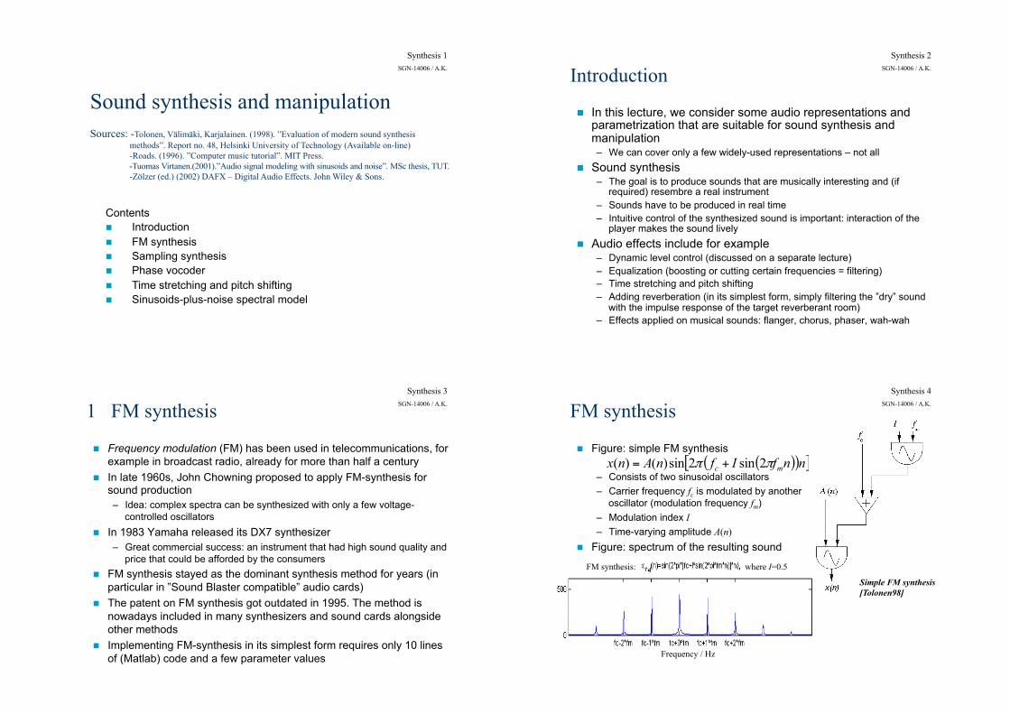
! Figure: simple FM synthesis – Consists of two sinusoidal oscillators – Carrier frequency fc is modulated by another
oscillator (modulation frequency fm) – Modulation index I – Time-varying amplitude A(n)
! Figure: spectrum of the resulting sound
Simple FM synthesis [Tolonen98]
( )( )[ ]nnfIfnAnx mc ππ 2sin2sin)()( +=
Frequency / Hz
FM synthesis: where I=0.5
Synthesis 5 SGN-14006 / A.K. FM synthesis
! The formula for FM synthesis can be also written as
– Note that here we modulate phase instead of frequency " more correct name would be phase modulation (PM)
– FM synthesis can be studies using the above formula, since phase is the integral of frequency and integral of sine is sine
" PM and FM produce essentially the same kind of sound – In analog devices, FM is used: PM is practical only digitally
( )[ ]nfInfnAnx mc ππ 2sin2sin)()( +=
Synthesis 6 SGN-14006 / A.K. FM synthesis
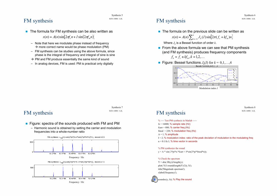
! The formula on the previous slide can be written as
Where Jk is a Bessel function of order k.
! From the above formula we can see that PM synthesis (and FM synthesis) produces frequency components
! Figure: Bessel functions Jk(I) for k = 0,1,…,4
[ ]∑∞
−∞=+=
k mck nkffIJnAnx )(2sin)()()( π
…,2,1, =±= kkfff mcn
Modulation index I
Synthesis 7 SGN-14006 / A.K. FM synthesis
! Figure: spectra of the sounds produced with FM and PM – Harmonic sound is obtained by setting the carrier and modulation
frequencies into a whole-number ratio
Frequency / Hz
Frequency / Hz
Synthesis 8 SGN-14006 / A.K. FM synthesis
% ---- Test PM synthesis in Matlab ----- fs = 16000; % sample rate (Hz) fcarr = 880; % carrier freq (Hz) fmod = 220; % modulation freq (Hz) A = 1; % amplitude I = 2; % modulation index: ratio of the peak deviation of modulation to the modulating freq n = 0:1/fs:1; % time vector in seconds % PM synthesize the sound y = A * sin( 2*pi*n.*fcarr + I*sin(2*pi*fmod*n)); % Check the spectrum Y = abs( fft(y))/length(y); plot( Y(1:round(length(Y)/2)), 'k'); title('Magnitude spectrum'); xlabel('frequency'); soundsc(y, fs); % Play the sound
Synthesis 9 SGN-14006 / A.K. FM synthesis: extensions
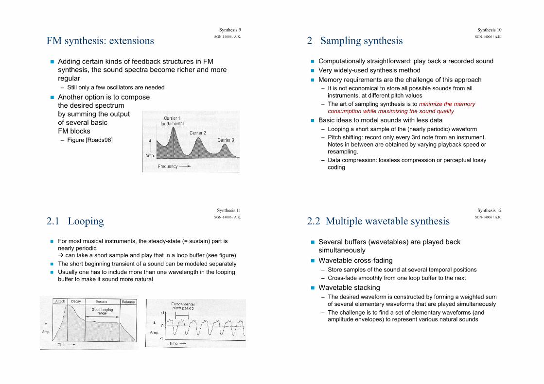
! Adding certain kinds of feedback structures in FM synthesis, the sound spectra become richer and more regular – Still only a few oscillators are needed
! Another option is to compose the desired spectrum by summing the output of several basic FM blocks – Figure [Roads96]
Synthesis 10 SGN-14006 / A.K. 2 Sampling synthesis
! Computationally straightforward: play back a recorded sound ! Very widely-used synthesis method ! Memory requirements are the challenge of this approach
– It is not economical to store all possible sounds from all instruments, at different pitch values
– The art of sampling synthesis is to minimize the memory consumption while maximizing the sound quality
! Basic ideas to model sounds with less data – Looping a short sample of the (nearly periodic) waveform – Pitch shifting: record only every 3rd note from an instrument.
Notes in between are obtained by varying playback speed or resampling.
– Data compression: lossless compression or perceptual lossy coding
Synthesis 11 SGN-14006 / A.K. 2.1 Looping
! For most musical instruments, the steady-state (= sustain) part is nearly periodic " can take a short sample and play that in a loop buffer (see figure)
! The short beginning transient of a sound can be modeled separately ! Usually one has to include more than one wavelength in the looping
buffer to make it sound more natural
Synthesis 12 SGN-14006 / A.K. 2.2 Multiple wavetable synthesis
! Several buffers (wavetables) are played back simultaneously
! Wavetable cross-fading – Store samples of the sound at several temporal positions – Cross-fade smoothly from one loop buffer to the next
! Wavetable stacking – The desired waveform is constructed by forming a weighted sum
of several elementary waveforms that are played simultaneously – The challenge is to find a set of elementary waveforms (and
amplitude envelopes) to represent various natural sounds
Synthesis 13 SGN-14006 / A.K. 3 Spectrum models
3.1 Additive synthesis ! Idea: construct a sound by summing sinusoidals
– The amplitudes and frequencies Ak and fk of individual sinusoids are slowly-varying
! In principle enables very high quality
! Drawback – Requires a lot of data
(time-varying parameters) – Large number of oscillators
! Figure: temporal evolution of the harmonic partials of a flute sound
( )[ ]∑=k
kk ttftAty π2sin)()(
Synthesis 14 SGN-14006 / A.K. 3.2 Phase vocoder
! Phase vocoder – ”vocoder” = voice coder: invented in the 60s when researching
speech compression methods – applications nowadays: audio time stretching, pitch shifting,
audio morphing, time-frequency domain processing
! General name for analysis-synthesis methods where – audio signal is represented as a sum of sinusoids – in addition to magnitudes and frequencies, also phases are
synthesized
! Usually implemented using short-time Fourier transform (STFT) – Described in the following
Synthesis 15 SGN-14006 / A.K. Phase vocoder
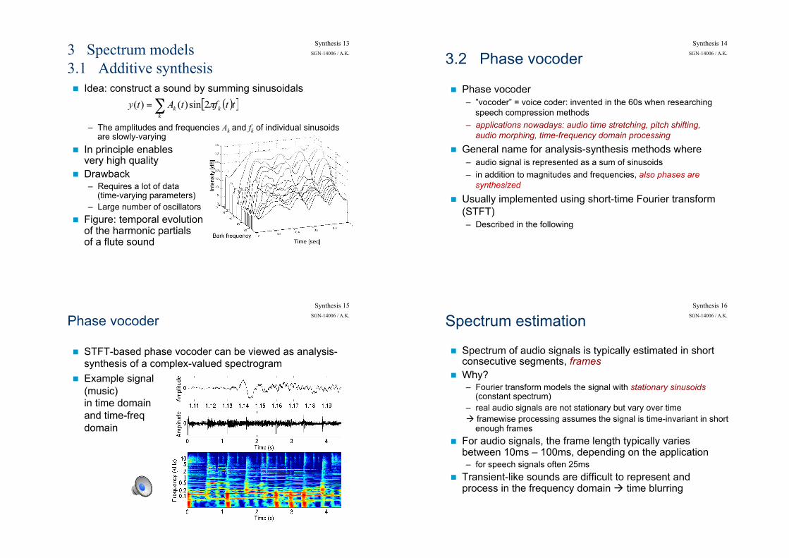
! STFT-based phase vocoder can be viewed as analysis-synthesis of a complex-valued spectrogram
! Example signal (music) in time domain and time-freq domain
Synthesis 16 SGN-14006 / A.K. Spectrum estimation
! Spectrum of audio signals is typically estimated in short consecutive segments, frames
! Why? – Fourier transform models the signal with stationary sinusoids
(constant spectrum) – real audio signals are not stationary but vary over time " framewise processing assumes the signal is time-invariant in short
enough frames ! For audio signals, the frame length typically varies
between 10ms – 100ms, depending on the application – for speech signals often 25ms
! Transient-like sounds are difficult to represent and process in the frequency domain " time blurring

Synthesis 17 SGN-14006 / A.K. Windowing
! Windowing is essential in frame-wise processing – weight the signal with a window function w(k) prior to transform – as a rule of thumb, windowing is always needed: one cannot just
take a short part of a signal without windowing
∑−
=
=1
0)()()(
N
n
nkmm WnwnxkX)()( nwnxm1,...,0),( −= Nnnxm
signal in frame m: windowed signal: short-time spectrum:
Synthesis 18 SGN-14006 / A.K. Windowing
! Example: spectrum of a sinusoid with/without windowing 1. No windowing (=rectangular window), sinusoid at a spectral bin 2. No windowing, random off-bin frequency " spectral blurring! 3. Hanning window, sinusoid at a spectral bin 4. Hanning window, random off-bin frequency " ok
! There are different types of windows, but most important is not to forget windowing altogether
Synthesis 19 SGN-14006 / A.K. Windowing in framewise processing
! Figure: Hanning windows – adjacent windows sum to unity when frames overlap 50% " all parts of the signal get an equal weight
– In each frame, the signal is weighted with the window function and short-time discrete Fourier transform is calculated
! This yields a spectrogram – complex spectrum in each frame over time
framewise processing
time freq
uenc
y
time (ms)
Synthesis 20 SGN-14006 / A.K. Windowing in analysis-synthesis systems
! Sine window (left panel below) is useful in analysis-synthesis systems – squared sine window equals the hanning window (middle panel)
! Sine windowing is done again in resynthesis to avoid artefacts at frame boundaries in the case that signal is manipulated in the f-domain – Figure below: 50% frame overlap leads to perfect reconstruction if nothing
is done at subbands
window
ing
DFT
signal in one frame ...
processing at subbands (freq. domain) ...
inverse DFT
window
ing
output
(overlap-add frames)

Synthesis 21 SGN-14006 / A.K. Reconstructing the time domain signal:
overlap-add technique ! Reconstructing a signal from its spectrogram:
1. inverse Fourier transform the spectrum of each frame back to time domain
2. apply windowing in each frame (e.g. sine or Hanning window) 3. successive frames are positioned to overlap 50% or more, and
summed sample-by-sample
Synthesis 22 SGN-14006 / A.K. Time stretching and pitch shifting
! Phase vocoder allows audio time stretching and pitch shifting ! Time strecthing
– change the time interval between frames during synthesis, OR althernatively, frames are copied or deleted at suitable intervals
– time-domain windowing has to be done carefully to avoid artefacts – phases are processed to keep phase time derivative unchanged
(duration • 2 " phases • 2) – in practice, some details are needed (see the code on next slide)
Synthesis 23 SGN-14006 / A.K. Time stretching and pitch shifting
! Time-stretching algorithm in a nutshell (stretching with ratio tStrRatio)
% interval between successive frames is different in analysis/synthesis winHopAn = round(0.7*winHopSyn); % slow-down audio since 0.7 < 1 tStrRatio = winHopSyn / winHopAn; % time-stretch ratio % frame-to-frame phase shift of different frequencies without stretching omega = 2*pi*winHopAn*[0:wLen-1]'/wLen; phi0 = zeros(wLen,1); psi = zeros(wLen,1); inInd = 0; outInd = 0; while inInd< length(audioIn)-wLen,
frame = audioIn(inInd+1:inInd+wLen).* winAn; f = fft(fftshift(frame)); delta_phi= omega + princarg(angle(f)-phi0-omega); phi0 = angle(f); psi = princarg(psi+delta_phi*tStrRatio); ft = (abs(f).* exp(i*psi)); frame = fftshift(real(ifft(ft))).*winSyn; audioOut(outInd+1:outInd+wLen) = ...
audioOut(outInd+1:outInd+wLen) + frame; inInd = inInd + winHopAn; outInd = outInd + winHopSyn;
end
% small function used in the code function phase=princarg(phase_in) phase=mod(phase_in+pi,-2*pi)+pi;
Synthesis 24 SGN-14006 / A.K. Time stretching and pitch shifting
! Pitch shifting – time-stretch first, then resample the signal so that duration becomes the
same again, but pitch changes – large changes make especially speech sound strange, because formants
(coarse specral envelope) are shifted too ! In spectrogram representation, sound can be flexibly processed
before returning to time domain – Filtering: multiply with frequency response – Morphing sounds: interpolate the magnitude and phase spectra of sounds
24 / klap

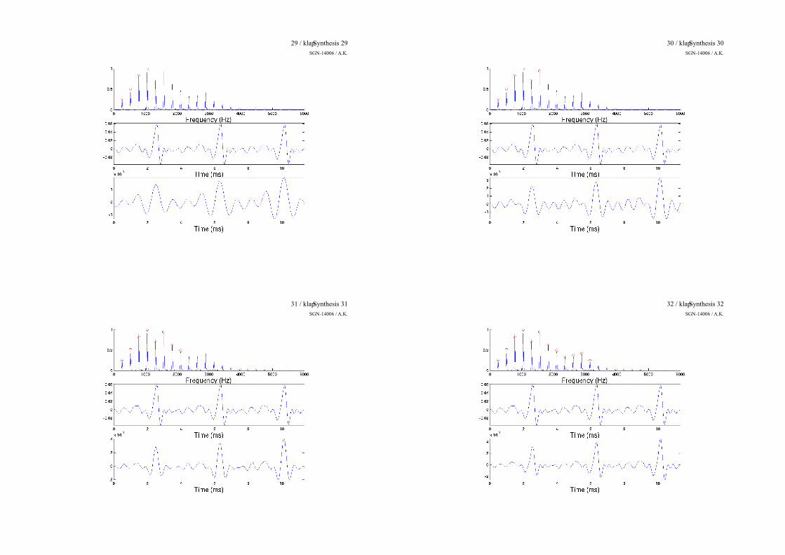
Synthesis 25 SGN-14006 / A.K. 3.3 Sinusoids plus noise model
! Signal model
" signal x(t) is represented with N sinusoids (freq, amplitude, phase) and noise residual r(t)
! Additive synthesis – according to Fourier theorem, any signal can be represented as a
sum of sinusoids – makes sense only for periodic signals, for which the amount of
sinusoids needed is small – non-deterministic part would require a large number of sinusoids
" use stochastic modeling
[ ] )()()(2cos)()(1
trtttftatxN
nnnn∑
=
++= ϕπ
Synthesis 26 SGN-14006 / A.K.
26 / klap
Synthesis 27 SGN-14006 / A.K.
27 / klap Synthesis 28 SGN-14006 / A.K.
28 / klap
Synthesis 29 SGN-14006 / A.K.
29 / klap Synthesis 30 SGN-14006 / A.K.
30 / klap
Synthesis 31 SGN-14006 / A.K.
31 / klap Synthesis 32 SGN-14006 / A.K.
32 / klap

Synthesis 33 SGN-14006 / A.K. Sinusoids+noise model
Analysis ! Block diagram
[Virtanen 2001] 1. detect sinusoids
in framewise spectra 2. estimate sinusoid
parameters and resynthesize
3. subtract sinusoids from original signal
4. model the noise residual
! We get – sinusoid parameters – noise level at
critical-band subbands
Synthesis 34 SGN-14006 / A.K. Sinusoids+noise model
Detecting and estimating sinusoids ! Block diagram: [Virtanen01] ! Spectral peaks are
interpreted as sinusoids 1. ”peak”: local maximum
in magnitude spectrum 2. peak frequency, amplitude,
and phase can be picked from the complex spectrum
! Tracking the peaks detected in successive frames " gives parameters of
a time-varying sinusoid " ”sinusoidal trajectory”
time
Synthesis 35 SGN-14006 / A.K. Sinusoids+noise model
Tracking the peaks ! If needed, spectral peaks in successive frames can be
associated and joined into time-vayring sinusoids " frequency, amplitude, and phases joined into curves
! Figure: peak tracking algorithm [Virtanen2001] – based e.g. on the track
derivatives; try to form a smooth track
– kill: if no continuation found, end the sinusoid
– birth: if spectral peak is not a continuation for an existing sinusoid, create a new one
Synthesis 36 SGN-14006 / A.K. Sinusoids+noise model
Synthesis of sinusoids ! Additive synthesis
! Often tracking the peaks is not necessary, but – synthesize sinusoids in each frame separately, keep the
parameters fixed in one frame – window the obtained signal with Hann window – overlap-add
[ ]∑=
+=N
nnnn tttftats
1
)()(2cos)()( ϕπ
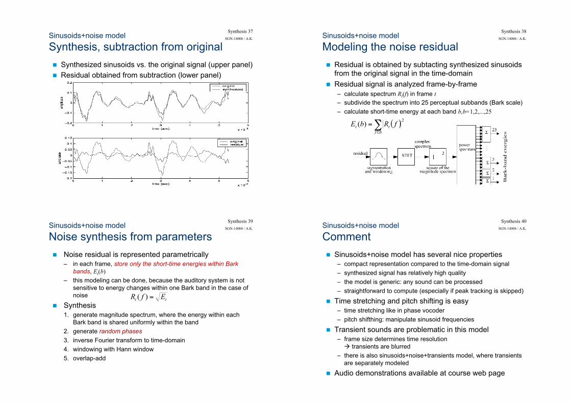
Synthesis 37 SGN-14006 / A.K. Sinusoids+noise model
Synthesis, subtraction from original ! Synthesized sinusoids vs. the original signal (upper panel) ! Residual obtained from subtraction (lower panel)
Synthesis 38 SGN-14006 / A.K. Sinusoids+noise model
Modeling the noise residual ! Residual is obtained by subtacting synthesized sinusoids
from the original signal in the time-domain ! Residual signal is analyzed frame-by-frame
– calculate spectrum Rt(f) in frame t – subdivide the spectrum into 25 perceptual subbands (Bark scale) – calculate short-time energy at each band b,b=1,2,...,25
( )2)( ∑∈
=bf
tt fRbE
Synthesis 39 SGN-14006 / A.K. Sinusoids+noise model
Noise synthesis from parameters ! Noise residual is represented parametrically
– in each frame, store only the short-time energies within Bark bands, Et(b)
– this modeling can be done, because the auditory system is not sensitive to energy changes within one Bark band in the case of noise
! Synthesis 1. generate magnitude spectrum, where the energy within each
Bark band is shared uniformly within the band 2. generate random phases 3. inverse Fourier transform to time-domain 4. windowing with Hann window 5. overlap-add
tt EfR =)(
Synthesis 40 SGN-14006 / A.K. Sinusoids+noise model
Comment ! Sinusoids+noise model has several nice properties
– compact representation compared to the time-domain signal – synthesized signal has relatively high quality – the model is generic: any sound can be processed – straightforward to compute (especially if peak tracking is skipped)
! Time stretching and pitch shifting is easy – time stretching like in phase vocoder – pitch shifthing: manipulate sinusoid frequencies
! Transient sounds are problematic in this model – frame size determines time resolution
" transients are blurred – there is also sinusoids+noise+transients model, where transients
are separately modeled
! Audio demonstrations available at course web page