symbolic and numerical computation for artificial … and numerical computation for artificial...
TRANSCRIPT
Symbolic and Numerical Computation for
Artificial Intelligence edited by
Bruce Randall Donald Department of Computer Science
Cornell University, USA
Deepak Kapur Department of Computer Science
State University of New York, USA
Joseph L. Mundy AI Laboratory
GE Corporate R&D, Schenectady, USA
Academic Press Harcourt Brace Jovanovich, Publishers
London San Diego New York Boston Sydney Tokyo Toronto
ACADEMIC PRESS LIMITED 24--28 Oval Road
London NW1
US edition published by ACADEMIC PRESS INC.
San Diego, CA 92101
Copyright © 1992 by ACADEMIC PRESS LIMITED
This book is printed on acid-free paper
All Rights Reserved No part of this book may be reproduced in any form, by photostat, microfilm or any other
means, without written permission from the publishers
A catalogue record for this book is available from the British Library
ISBN 0-12-220535-9
Printed and Bound in Great Britain by The University Press, Cambridge
Chapter 13
An Interactive Symbolic-Numeric Interface to Parallel ELLPACK for Building General PDE
Solvers
Sanjiva Weerawarana, Elias N. Houstis, John R. Rice t
Department of Computer Science
Purdue University
West Lafayette, IN 47907
In this paper we describe an interactive symbolic-numeric interface framework (editor) to the ELLPACK partial differential equation (PDE) system for building PDE solvers for a much broader range of applications. The domain of applicability of ELLPACK and its parallel version(/ /ELLPACK) is restricted to second order linear elliptic boundary value problems. This editor allows the specification of nonlinear initial and boundary value PDE problems. The editor applies hybrid symbolic-numeric techniques at the PDE problem level to automatically reduce them to a sequence of linear elliptic PDEs. The result of this preprocessing is recorded in the form of an ELLPACK program. Several examples are presented to demonstrate the functionality and applicability of this interface framework, and the efficiency of the underlying solution methods.
1. Introduction
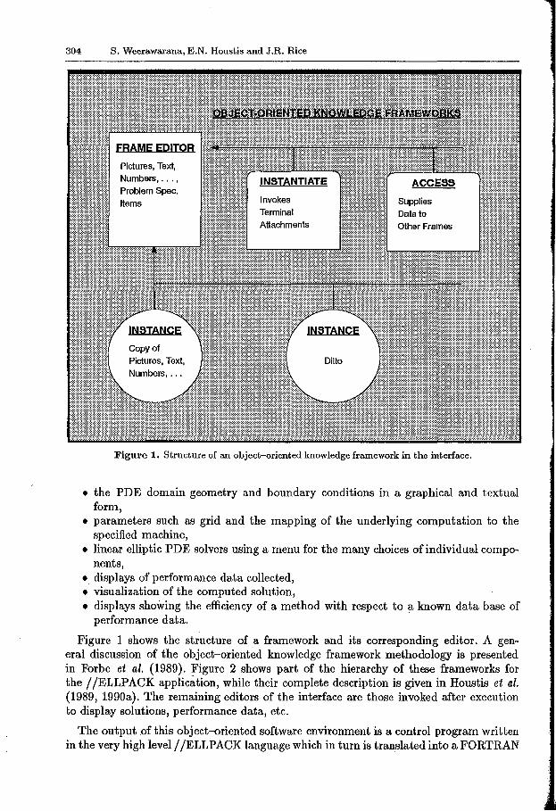
ELLPACK is a high level software environment for specifying linear elliptic second order boundary value problems and their solvers. The solvers are built out of an extensive library of modules that correspond to the various phases of the numerical processes for these types of PDE problems. A detailed description of the ELLPACK system for sequential machines is given in Rice and Boisvert (1985). The system is currently being extended to accommodate PDE problems which may be nonlinear, second order in space and parabolic or hyperbolic in time. The extension also includes facilities to specify or select pairs of parallel algorithms and architectures. We use an object-oriented knowledge framework (editor) interface which allows the user to specify:
• linear/nonlinear PDE boundary /initial value problems in a natural form,
t This research was supported in part by AFOSR 88-0234, ARO grant DAAG29-83-K-0026, NSF grant CCF-8619817 and ESPRIT project GENESIS.
304 S. Weerawarana, E.N. Houstis and J.R. Rice
Pictures, Text,
Numbers, ... , Problem Spec.
Items Invokes Terminal
Attachments
Supplies
Data to
Other Frames
Figure 1. Structure of an object-oriented knowledge framework in the interface.
• the PDE domain geometry and boundary conditions in a graphical and textual form,
• parameters such as grid and the mapping of the underlying computation to the specified machine,
• linear elliptic PDE solvers using a menu for the many choices of individual compo-nents,
• displays of performance data collected, • visualization of the computed solution, • displays showing the efficiency of a method with respect to a known data base of
performance data.
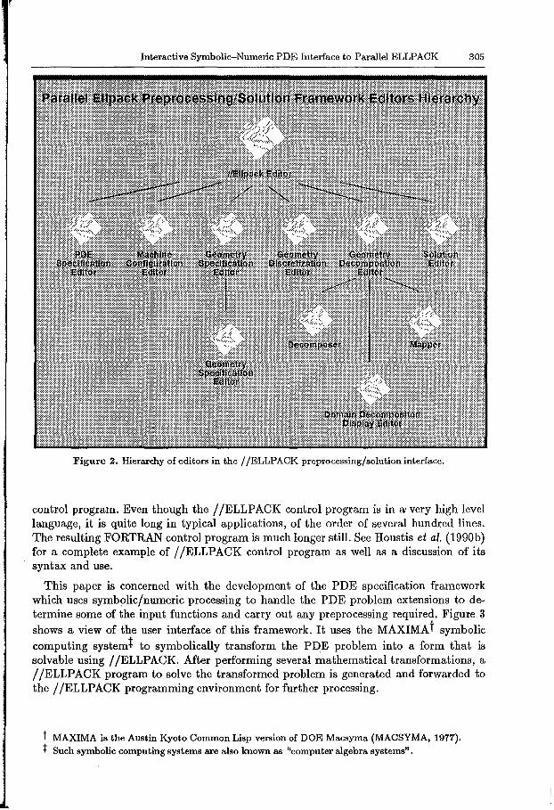
Figure 1 shows the structure of a framework and its corresponding editor. A general discussion of the object-oriented knowledge framework methodology is presented in Forbe et al. (1989). Figure 2 shows part of the hierarchy of these frameworks for the I IELLPACK application, while their complete description is given in Houstis et al. (1989, 1990a). The remaining editors of the interface are those invoked after execution to display solutions, performance data, etc.
The output of this object-oriented software environment is a control program written in the very high level I /ELLPACK language which in turn is translated into a FORTRAN
Interactive Symbolic-Numeric PDE Interface to Parallel ELLPACK 305
Figure 2. Hierarchy of editors in the/ /ELLPACK preprocessing/solution interface.
control program. Even though the / /ELLPACK control program is in a• very high level language, it is quite long in typical applications, of the order of several hundred lines. The resulting FORTRAN control program is much longer still. See Houstis et al. (1990b) for a complete example of/ /ELLPACK control program as well as a discussion of its syntax and use.
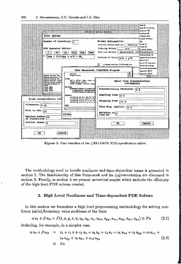
This paper is concerned with the development of the PDE specification framework which uses symbolic/numeric processing to handle the PDE problem extensions to determine some of the input functions and carry out any preprocessing required. Figure 3 shows a view of the user interface of this framework. It uses the MAXIMA t symbolic computing system+ to symbolically transform the PDE problem into a form that is solvable using / /ELLPACK. After performing several mathematical transformations, a / /ELLPACK program to solve the transformed problem is generated and forwarded to the/ /ELLPACK programming environment for further processing.
t MAXIMA is the Austin Kyoto Common Lisp version of DOE Macsyma (MACSYMA, 1977). :j: Such symbolic computing systems are also known as "computer algebra systems".
306 S. Weerawarana, E.N. Houstis and J.R. Rice
stopping Time: ;"i·a·:ii .................................................... j o,.,.,.,.,.,.,.,.,.,.,.,.,.,.,.,.,.,.,.u,•o•o•~rro•,.,._.,.,.,.,.,.,.,.,.,.,.,.,.,.,.,.,.,.,.,.,.,.,.,.,.,.,.,.;.,.,/
Tima step (del tat) : [~:::~:::::::::::::~:::::::::~::::::::::::::::::::;
r~t~~~ at[?.:::::::::::::::::::::::::::~:~::~::.:~::::~~:::::::::::::::::::;
Initial Guess: [~.:.:.:.:.:.:~~~:.·.::::.:.:::.::.:.:.::.:.::.:.:.:.:.:.:.:.:~.!
Figure 3. User interface of the/ /ELLPACK PDE specification editor.
The methodology used to handle nonlinear and time-dependent terms is presented in section 2. The functionality of this framework and its implementation are discussed in section 3. Finally, in section 4 we present numerical results which indicate the efficiency of the high level PDE solvers created.
2. High Level Nonlinear and Time-dependent PDE Solvers
In this section we formulate a high level preprocessing methodology for solving nonlinear initial/boundary value problems of the form
aUt+ (3 Utt = F(t,rn, y, z, u, U:u, Uy, Uz, U:u:!J, Uyy, Uzz, U:uy, U:uz, Uyz) = Fu
including, for example, in a simpler case,
C¥Ut + f3Utt Co+ C1 U + C2 U:u + C3 Uy + C4 Uz + C5 U:u:u + C6 Uyy + C7Uzz + Cg U:uy + Cg U:uz + C10 Uyz
Lu
(2.1)
(2.2)
Interactive Symbolic-Numeric PDE Interface to Parallel ELLPAOK 307
Problems (2.1) and (2.2) are defined on (0, T] x n with 0 C ~3 and are subject to boundary conditions
Gu =: G(t, x, y, z, u, Ux, Uy, Uz) = '!f;(t)
or, again in the simpler case,
Bu = do + d1 u + d2 Ux + ds Uy = 0
on the boundary of n, and initial conditions at t = 0
u(O,x,y,z) = ¢(x,y,z).
(2.3)
(2.4)
(2.5)
The coefficients c; and d; may depend on (x, y, z) and yet the problem remains in the class of linear PDEs that / /ELLPACK currently assumes. The coefficients of L and B could be functions of the solution u, making a semi-linear problem not in the class that f /ELLPACK currently assumes. The parameters ex and f3 are chosen to make the equation (2.1) elliptic (ex= 0,{3 = 0), parabolic (ex = 1,{3 = 0) and hyperbolic (a=0,f3=1).
2.1. NONLINEAR PDE SOLVERS
The traditional way to handle nonlinear PDE problems numerically is to discretize them first with an appropriate method and then solve the corresponding nonlinear algebraic' equations. A non-traditional alternative is to apply a nonlinear methodology directly on the continuous PDE equations and boundary conditions. This approach reduces the original nonlinear PDE problem to a sequence of linear PDEs which must be solved by iteration starting with some initial guess. Under certain general assumptions we can show that the two approaches are equivalent. Another advantage of the second approach is the ability to utilize existing linear PDE solvers without any modification. Its disadvantage is that the user has to define and implement the nonlinear process at the program control (PDE operator) level and carry out the symbolic processing required. Rice has tested this methodology (Rice, 1983; Rice and Boisvert, 1985) ·by constructing special ELLPACK templates, which implement nonlinear and time-dependent high level solvers by embedding FORTRAN code into ELLPACK. In order to separate the user from the PDE problem specification and PDE preprocessing/solution phases, we have developed a knowledge-based editor whi~4 automatically generates these templates from given specifications and carries out the needed symbolic processing. The/ /ELLPACK system already has a natural interface to MAXIMA and / /ELLPACK and now implements two of the most often used nonlinear approaches, the Picard and Newton's iterations. Their formulation at the PDE problem level has appeared in Rice and Boisvert (1985). For completeness, we present it here.
2.1.1. PICARD ITERATION FOR NONLINEAR PROBLEMS
In order to apply Picard iteration, one rewrites the equations F(u) = 0 and G(u) = 0 into the form L(u)u = f(u), and B(u)u = g(u) and then uses the iteration
308 S. Weerawarana, E.N. Houstis and J.R. Rice
l"i.~:i~···~~~~~·~····"'''"'''"'''"''""'""''"'''"'''"''''"''"'''''''''"''''''''"''"''""'''""'''"''''''""'''''''''"""''""''"'''""'''''"''""''"~~i~"'
r~~·~~~; .. ~;· .. ~~~;~~~;~·~i.;.: ... :.-.:r ....................................... ~~~~~~ .. ~~;~;~~~~~~·~ ........... · ... ...... .. ................... ..
" Discretization Method: f'w'""s:p;;"j~t'"'st~j:'""'"""G'"·~
.. !PDE Ope~ato~ Edito~·. . • • • Indexing Method: c···········A;··;; ..... ., ......... 5.'! l r····u'''j DE] []JL] ~ !1§U ("u~~·j Solution Method: r······--·;~~~'bi"si""""''''r€} f 1:~ + Uyy = U"2 * (x"2+y"2) * e"(-x*y) !
Solution to force:f l : ...................................................................................................... ...J
~ Linearization Information ~ Time Discretization Information
~ Generate //ELLPACK Program
~~~~'l~·~r-1::;::~. 'r.~;,~:S" ""'·~·~··· I ... JJ ..... l .. ,:,.l ... i·.·'
f pde * 1 Is not tl~e-d~pendent, :.: f. pde t+ 1 is non-linear. ~ ..... f: Generating progra"•• i ~::::~ r (DB) DONE i !'''!! i' (C7) " i ! i lii.!:~;::::::;;:::::~:::::::::::::::::~::::::~:::::::::::::;~:::::;:::::::::::::::~:;::::~;:::::E::::~:::~:::~::~;:::::~::::;;;;::;~:;:::::::~::::::::::::::~::::::;:::::~:::~~~:::::::;~:::::::~:;::::~::::::::::::::::::~::~~~~:::0.:::~:::::0..~~~::::::~:; 1~1
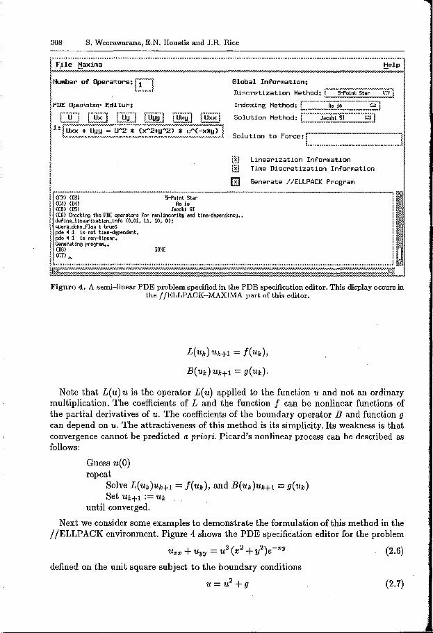
Figure 4. A semi-linear PDE problem specified in the PDE specification editor. This display occurs in the/ /ELLPACK-MAXIMA part of this editor.
L(u,~:)uk+l = f(u.~:), B(u,~:)uk+l = g(u,~:).
Note that L(u)u is the operator L(u) applied to the function u and not an ordinary multiplication. The coefficients of L and the function f can be nonlinear functions of the partial derivatives of u. The coefficients of the boundary operator B and function g can depend on u. The attractiveness of this method is its simplicity. Its weakness is that convergence cannot be predicted a priori. Picard's nonlinear process can be described as follows:
Guess u(O) repeat
Solve L(uk)uk+l = f(u.~:), and B(uk)uk+l = g(uk) Set Uk+l := u,~:
until converged.
Next we consider some_ examples to demonstrate the formulation of this method in the / /ELLPACK environment. Figure 4 shows the PDE specification editor for the problem
u~~ + Uyy = u2 (a:2 + y2)e-xy
defined on the unit square subject to the boundary conditions
u = u2 +g
(2.6)
(2.7)
Interactive Symbolic-Numeric PDE Interface to Parallel ELLPACK 309
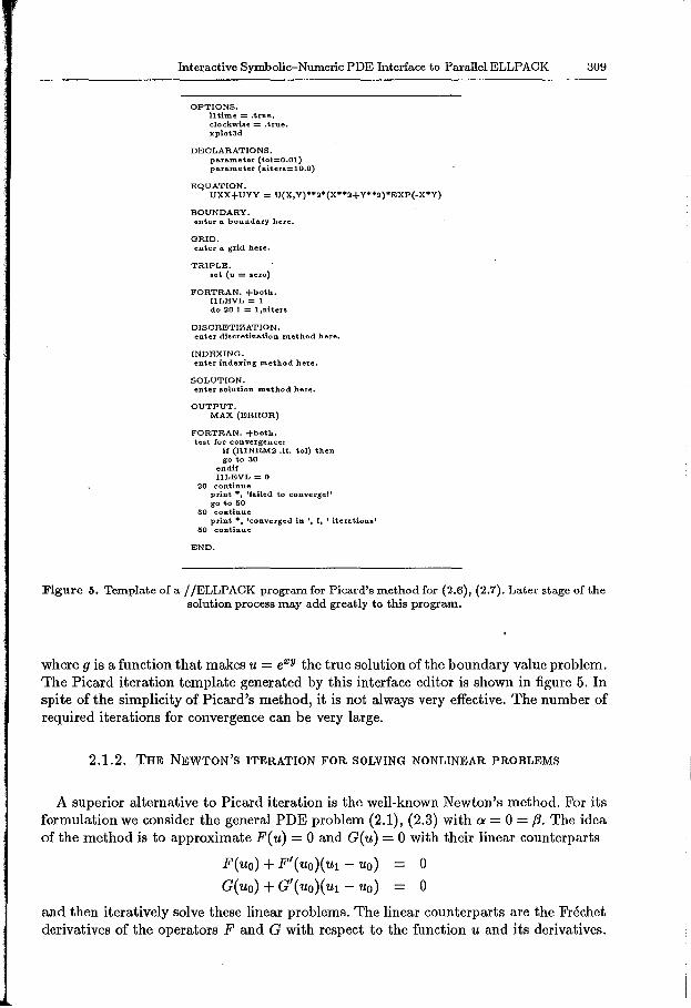
OPTIONS. 11 time = .true, clockwise = .true. xplot3d
DECLARATIONS. parameter (tol=O.Ol) pa.ra.meter (niters=lO.O)
EQUATION. UXX+UYY = U(X,Y) 002°(X**2+Y* 0 2)*EXP(-X*Y)
BOUNDARY. enter a. boundary here,
GRID. enter a. grid here.
TRIPLE. set (u =zero)
FORTRAN. +both. llLEVL = 1 do 20 I = 1 ,niters
DISCRETIZATION. enter discretization method here,
INDEXING. enter indexing method here.
SOLUTION. enter solution method here.
OUTPUT. MAX (ERROR)
FORTRAN. +both. test for convergence:
if (R1NRM2 .It. to!) then go to 30
endif llLEVL = 0
20 continue print •, 'fa.iled to converge!' go to 50
30 continue print*, 'converged in 1
1 I, 1 iterations' 50 continue
END.
Figure 5. Template of a/ /ELLPACK program for Picard's method for (2.6), (2.7). Later stage of the solution process may add greatly to this program.
where g is a function that makes u = exy the true solution of the boundary value problem. The Picard iteration template generated by this interface editor is shown in figure 5. In spite of the simplicity of Picard's method, it is not always very effective. The number of required iterations for convergence can be very large.
2.1.2. THE NEWTON'S ITERATION FOR SOLVING NONLINEAR PROBLEMS
A superior alternative to Picard iteration is the well-known Newton's method. For its formulation we consider the general PDE problem (2.1), (2.3) with a= 0 = {3. The idea of the method is to approximate F(u) = 0 and G(u) = 0 with their linear counterparts
F(uo) + F'(uo)(ul- uo) 0
G(uo) + G'(uo)(ul- uo) 0
and then iteratively solve these linear problems. The linear counterparts are the Frechet derivatives of the operators F and G with respect to the function u and its derivatives.
310 S. Weerawarana, E.N. Houstis and J.R. Rice
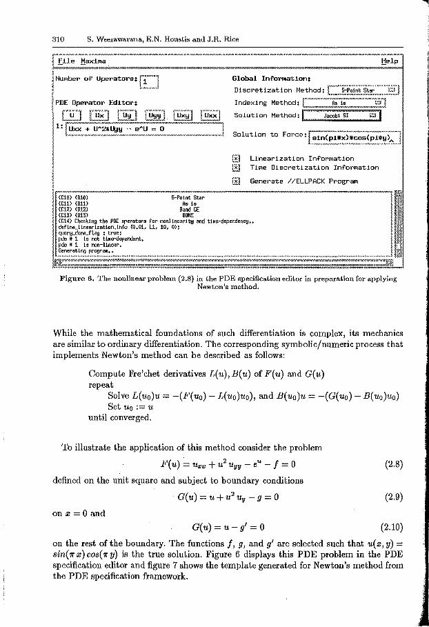
r··.Ei'i;·······.M;~;_;;···.······--····w····················································--·············································--············································w··m·······m·····--···························--·····--·········--···
F""'"'«« .... ~~ .. ~ .... «-: .. ~~ .... «":";~":7.o;-;o: ......... ••••••••• «~~~~~~ .......................... ................ "7.~ ••
i! Humber of' Operators: p."""i Global Inf'ormation:
~ .. :. . ......... ..l Discretization Method: f'"'"S:ii.~i~t··st~~··········:;s·J· " . ~ ...................................... . j PDE Operator Editor: Indexing Method: r·········""····.wo···;;;···j·;····--···················;;:5···'!
1 []] @D Q!ii] f"u!l·;;···i [§] U§J solution Method: r::::::::{e~;x::~c:::::::::§] 1
1 ~·~,,~~,~-·~.:· ... ~:~~,~~:~N,:N,:<:~,•,•,•:,.,,?,:,._..,.,•,•NNNm,•,•m,:<.•.w.w,•,•,,J ~ ~ ~
j iil Linearization Information !, lliJ Time Discl"etization Information
I ~fut ~:::lt ----~0~~\;tar iiJ Generate //ELLPACK Pl"ogram
I ~!~~~~ir::~:::: u: ~·:;~: "~--·· 1.\ r1.
~ pde H 1 Is non-linear, . ~ Generating progra~.. ~ ~
!!&;;;,~:f::::~::,;,;;;;;,;;,;;,;~;i:~::;:;::;~:f:~;f:~~::;::~:::~~:::::::::~::;:~f::~::::::f::::::::::::::~~::::;:::::0;::;::f:;:~:::;:::;~:~::~::::::~::::;~~:::~;~~:::;~:~,;;,;~;pf'::l Figure 6. The nonlinear problem (2.8) in the PDE specification editor in preparation for applying
Newton's method.
While the mathematical foundations of such differentiation is complex, its mechanics are similar to ordinary differentiation. The corresponding symbolic/numeric process that implements Newton's method can be described as follows:
Compute Fre'chet derivatives L(u), B(u) of F(u) and G(u) repeat
Solve L(uo)u = -(F(uo)- L(uo)uo), and B(uo)u = -(G(uo)- B(uo)uo) Set uo := u
until converged.
To illustrate the application of this method consider the problem
F(u) = U 111111 + u2 Uyy- eu- f = 0
defined on the unit square and subject to boundary conditions
· G(u) = u + u2 uy- g = 0
on x = 0 and
G( u) = u - g' = 0
(2.8)
(2.9)
(2.10)
on the rest of the boundary. The functions/, g, and g' are selected such that u(x, y) = sin( 1r x) cos( 1r y) is the true solution. Figure 6 displays this PDE problem in the PDE specification editor and figure 7 shows the template generated for Newton's method from the PDE specification framework.
Interactive Symbolic-Numeric PDE Interface to Parallel ELLPACK 311
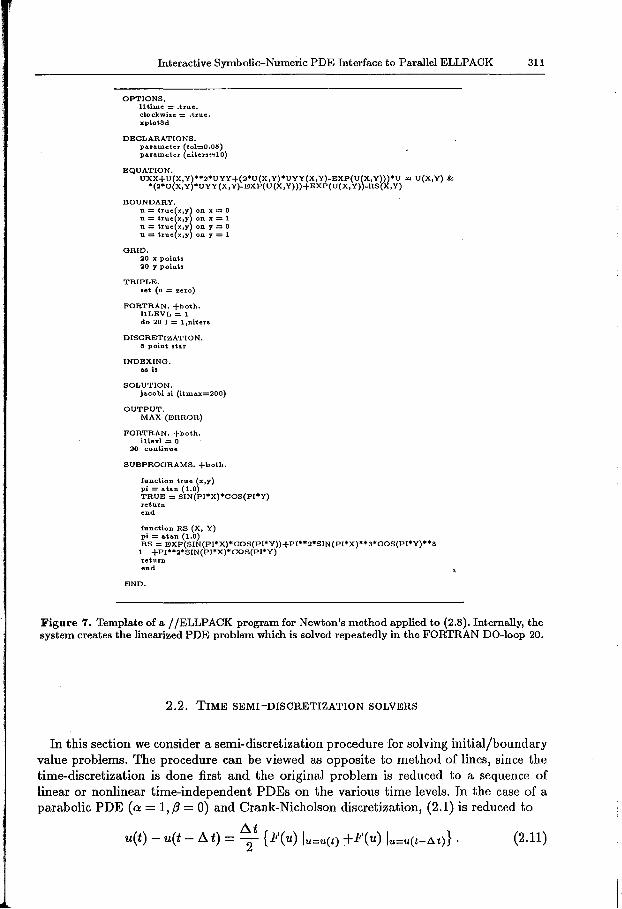
OPTIONS, 11 time = .true:. clockwise = ,true. xplot3d
DECLARATIONS. pa.rameter (tol=O.O.S) parameter (niters=lO)
EQUATION. UXX+U(X,Y)••2•UYV+(2•U(X,Y)•UYY(X,Y)-EXP(U(X,Y)))•U = U(X,Y) &
•(2•U(X,Y)•UYY(X,Y)-EXP(U(X,Y)))+EXP(U(X,Y))-RS(X,Y)
BOUNDARY. u = true(x,y) on x = 0 u = true(x,y) on x = 1 u = true(x,y) on y = 0 u = hue(x,y) on y = 1
GRID. 20 x points 20 y points
TRIPLE. set (u = zero)
FORTRAN. +both. llLEVL = 1 do 20 1 = 1 ,nit era
DISCRETIZATION. 5 point sta.r
INDEXING. &B is
SOLUTION. jacobi si (itma.x=200)
OUTPUT. MAX (ERROR)
FORTRAN. +both. illevl = 0
20 continue
SUBPROGRAMS. +both.
function true (x,y) pi= abn (1.0) TRUE = SIN(PI•x)•COS(PI*Y) return end
function RS (X, Y) pi = atan (1.0) RS = EXP(SIN(PI•X)*COS(PI•Y))+PI••2•SIN(PI•X)••a•COS(PI•Y)••a
1 +PI••2•SIN(PI•x)•coS(PI•Y) return end
END.
Figure 7. Template of a/ /ELLPACK program for Newton's method applied to (2.8).1nternally, the system creates the linearized PDE problem which is solved repeatedly in the FORTRAN DO-loop 20.
2.2. TIME SEMI-DISCRETIZATION SOLVERS
In this section we consider a semi-discretization procedure for solving initial/boundary value problems. The procedure can be viewed as opposite to method of lines, since the time-discretization is done first and the original problem is reduced to a sequence of linear or nonlinear time-independent PDEs on the various time levels. In the case of a parabolic PDE (a= 1, f3 = 0) and Crank-Nicholson discretization, (2.1) is reduced to
D..t u(t)- u(t- ~ t) = 2 { F(u) lu=u(t) +F(u) lu=u(t-~t)} · (2.11)
312 S. Weerawarana, E.N. Houstis and J.R. Rice
Note that we have suppressed the space variables and derivatives of u in the above equation. Assuming that the solution and its derivatives are known at thet-A t level, then the nonlinear PDE with respect to u(t) is solved over the domain Q with boundary conditions
G(u(t)) = ,P(t).
To illustrate this approach, we consider the equation
Ut = )rfl(u)ux)x + v (¢(u)uv)y - f(u)ux- g(u)uy + h un un
·defined on (0, T] X (unit square) subject to Dirichlet boundary conditions
u = true(t, x, y)
on the boundary of Q and initial conditions u = true(O, x, y).
(2.12)
(2.13)
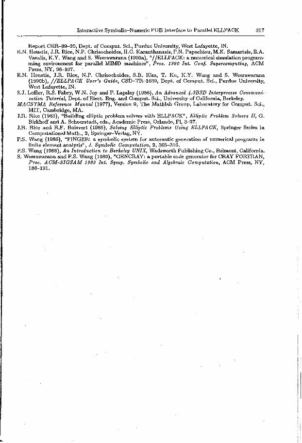
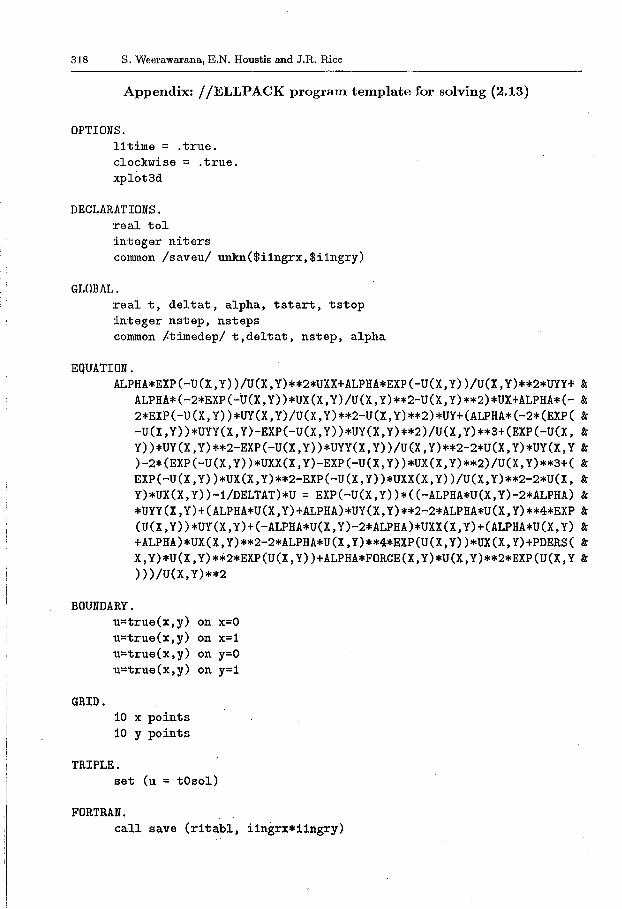
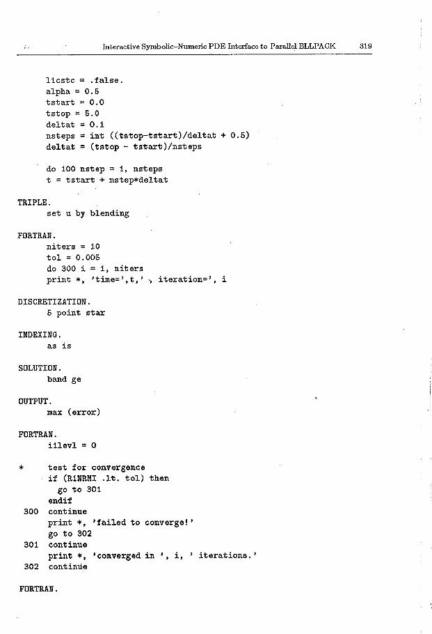
The equation is parametrized with respect to v, </J, n, j, and g. The function his chosen so that a given function true(t; x, y) is the solution of the PDE problem. The appendix shows the template for solving (2.13) with v = 1, t/J( u) = e-u, n = 2, f = g = u2 and true(t, x, y) = t + x + y.
3. A Symbolic/Numeric Interface for Nonlinear/Time-dependent PDEs
We have developed a PDE specification editor that is an interface between MAXIMA and / /ELLPACK. This editor implements some of the methodologies described. earlier to transform a nonlinear and/or time-dependent PDE into a sequence of elliptic PDEs that are accepted by / /ELLPACK. It is implemented in C and Lisp as an independent tool that uses simple protocols to communicate with MAXIMA and/ /ELLPACK. The graphical interface is built on top of the X Window System using the Motif widget set.
3.1. USER SPECIFICATION OF THE PDE OPERATOR
The PDE specification editor produces a / /ELLPACK program template that is further specialized by other editors of the / /ELLPACK Programming Environment. The only required information that the user must provide to the editor is the actual PDE operator. If the PDE is nonlinear, then the editor will ask for additional information to generate code for the iterative solution of the linearized PDE. Similarly, additional information is requested if the PDE is time-dependent; Other parameters of the the generated program (such as operator discretization method, and algebraic system indexing and solving methods) can also be specified via menu item selection.
The PDE operator editor window is a simple Emacs-like edit buffer where the PDE operator is entered. A sy~tem of PDEs can be specified by changing the number of PDEs from the default value of one. Another edit window allows one to specify a function that the PDE must be made to satisfy. This is achieved by perturbing the PDE by adding a term which forces the modified PDE to exactly (i.e. analytically) satisfy the specified function. This feature is extremely useful when one is attempting to debug a discretization
Interactive Symbolic-Numeric PDE Interface to Parallel ELLPACK 313
method, for example. We used this feature extensively during the development of this interface to verify· correctness of the generated code.
The other main component of the editor is the MAXIMA window. This is the trace window for MAXIMA and is not for direct user input. All communication between MAXIMA and the editor are echoed to this window so that progress can be monitored. Also, this window provides access to MAXIMA (for those users who are familiar with it) to manipulate the PDE problem data as needed.
Once the operator is defined, the user asks the editor to generate a I IELLPACK program by clicking on the Generate //ELLPACK Program button. At this time, the PDE is sent to MAXIMA for symbolic processing. MAXIMA interprets the operator and decides whether it is nonlinear, time-dependent etc. If the operator is nonlinear, a message is sent to the editor requesting it to ask for more information from the user and then forward the additional information to MAXIMA. Finally, the generated //ELLPACK program is sent to the editor which forwards it to the //ELLPACK programming environment. A similar transaction takes place in the case of parabolic/hyperbolic PDEs.
3.2. LINEARIZATION AND TIME DISCRETIZATION METHODOLOGY
If the given operator is found to be nonlinear, then it is linearized in the manner outlined in section 2.1.2 using MAXIMA's symbolic differentiation capability. If the operator is time-dependent, then the time-derivatives are discretized using one of several methods (for example, Crank-Nicholson discretization). Additional information for linearization and/or time-discretization is requested from the user by sending a message from MAXIMA to the editor. The editor then opens a window and gets the information from the user.
If the PDE is found to be nonlinear, a message is sent to the editor requesting it to ask the user for more information. The information that is requested currently includes the tolerance (to be used to check whether a satisfactory solution has been found), the maximum number of iterations to perform before aborting, the norm to' use to check for convergence and finally the initial guess. We plan to integrate knowledge-based assistance into this editor to automatically provide values for these parameters based on experience and other empirical data, if the user so desires.
For time-dependent PDEs, we allow the user to select one of several time-discretization methods, though it is always possible to define any discretization scheme directly using MAXIMA's symbolic manipulation capabilities. As I /ELLPACK's data structures only provide convenient mechanisms for 2-stage time-discretizations, we currently limit the user to them. We are examining convenient implementation methods for k-stage techniques also. The other parameters that are involved with the time-discretization stage are the starting time (t0), the solution uo at time to, the ending time (tend), and the time step. As with nonlinear PDEs, we expect to integrate knowledge-based assistance to select the time step needed to obtain some requested tolerance.
Once all the necessary parameters are specified, a I /ELLPACK program is generated. For nonlinear problems, this program iteratively improves an initial guess until some convergence criteria has been met. For time-dependent problems, the program steps along the time axis solving an elliptic problem at each step. If the operator is both time-
314 S. Weerawarana, E.N. Houstis and J.R. Rice
dependent and nonlinear, then the outer loop iterates over time while the inner loop iterates to solve the linearized elliptic PDE at each time step. The generated program is a I IELLPACK program which includes all necessary FORTRAN code. For example, FORTRAN functions are generated to compute derivatives of the initial conditions.
3.3. PDE SPECIFICATION EDITOR - MAXIMA INTERFACE
MAXIMA is a large, Lisp-based, interactive system that expects the user to type in expressions to be evaluated and printed. MAXIMA can be programmed in a high level language (MACSYMA, 1977) and in Lisp. In the PDE Specification Editor, MAXIMA runs as a separate process, possibly on a different host machine. The processes are connected via three sockets (Lefller et al., 1986); one to the standard input stream of MAXIMA, one to the standard output and standard error streams, and the other to a special connection to pass messages between MAXIMA and the editor. The MAXIMA functions we have implemented communicate with the editor using this third connection in a simple prot~col.
The user does not deal with MAXIMA directly but, instead, deals with the PDE Specification Editor. The editor provides very high level access to the transformations discussed earlier via menu choices and button clicks.
The PDE operator is entered symbolically in the PDE Operator Editor window. Similarly, the forcing solution (if any) is entered in another window. When the user clicks on the Generate / /ELLPACK Program button, messages are sent from the editor to MAXIMA giving it the necessary commands. If more information is needed, MAXIMA sends messages to the editor asking for the additional information. If what MAXIMA is asking for is not known, then the user is queried for the additional information. Once the information is available, it is forwarded to MAXIMA as another message. Finally, the generated I IELLPACK program is sent to the editor as a message from MAXIMA.
3.4. FORTRAN CODE GENERATION FROM MAXIMA
The I IELLPACK language allows one to use arbitrary FORTRAN functions (for boundary conditions, the PDE operator etc.) that are defined in a separate segment of the I IELLPACK file. This feature is used in the programs generated by the PDE Specification Editor to implement the true solution forcing capability, for example.
MAXIMA has simple FORTRAN code generation capabilities to generate FORTRAN code for expressions. We have extended this into a rudimentary code generation capability to generate the FORTRAN code we currently need (including loops, control structures and subprograms), using "print" statements. Since this technique does not allow one to manipulate the generated code, we will be integrating an automatic code generation system, GENCRAY (Weerawarana and Wang, 1989), to provide a flexible code generation capability.
The ability to manipulate generated FORTRAN code is very useful when dealing with PDEs that are both nonlinear and time-dependent, for example. Furthermore, since we
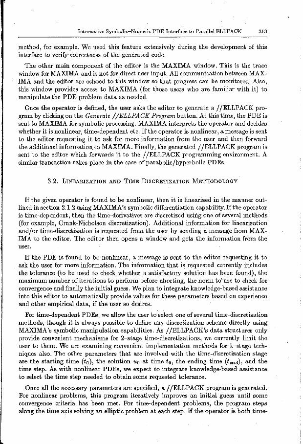
Interactive Symbolic-Numeric PDE Interface to Parallel ELLPACK 315
iterations iierrorlloo
1 6.767E-02 2 1.001E-02 3 1.466E-03 4 2.527E-04 5 5.215E-06 6 3.806E-05 10 ~ 3.329E-05
Table 1. The convergence of Picard's method for PDE (2.8) (with L( u) = Uxa: + u 2 * Uyy) defined on the unit square with Dirichlet boundary conditions and true solution u(x, y) = sin(1r x) cos('rr y). The computation uses ~x = ~y = 0.05.
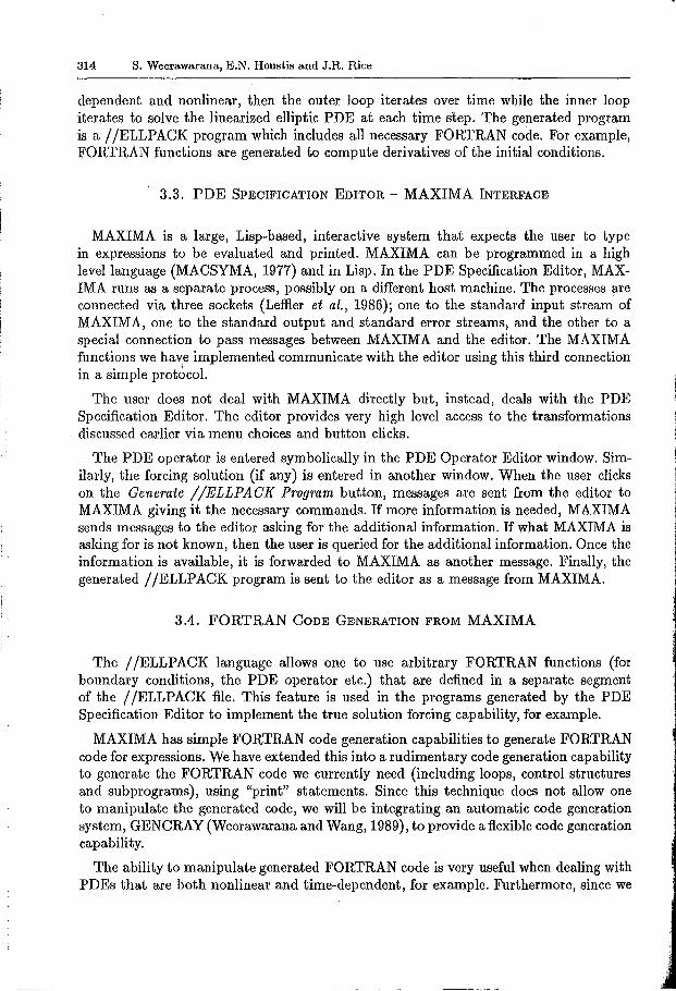
iterations llerrorlloo
1 1.804E-02 2 8.486E-04 3 3.749E-05 4 3.663E-05 5 3.725E-05
10 3.710E-05
'fable 2. The convergence of Newton's method for PDE (2.8) defined on the unit square with Dirichlet boundary conditions and true solution u(x,y) = sin(1rx)cos(1ry).
The computation uses ~x = ~y = 0.05.
intend to extend this editor to handle systems of PDEs as well, we need the ability to manipulate generated FORTRAN or/ /ELLPACK code conveniently.
4. Numerical Examples
Tables 1 and 2 indicate the error of five-point star approximations in the solution of PDE problem (2.8), coupled with Picard and Newton iterations, respectively. The approximations are computed using a 20x20 grid and measured in the L 00 norm. The numerical results confirm that the Picard method needs more iterations to reach the actual level of discretization error. This is in agreement with the theoretical behavior of the two methods.
The solution of the PDE problem (2.13) was selected so that it will coincide with the discrete approximation on a 10x10 grid. In table 3, we list the discretization error measured in the L00 norm. These results indicate that no accuracy is lost due to the linearization procedure used, and that the error remains at the single precision round-off error after several iterations and time levels.
In both PDE problems we have assumed Dirichlet boundary conditions and the JacobiSI method was used to solve the linear finite difference equations.
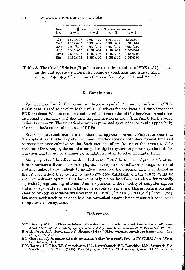
316 S. Weerawarana, E.N. Houstis and J.R. Rice
time llerrorlloo after k Newton iterations level k - 1 k - 2 k - 3 k - 5
llt 21lt 31lt 51lt 101lt 501lt
3.576E-07 4.172E-07 5.960E-07 5.960E-07 9.536E-07 1.192E-05
5.960E-07 5.960E-07 5.960E-07 7.152E-07 1.192E-06 1.096E-05
4.768E-07 5.960E-07 5.960E-07 7.152E-07 1.192E-06 1.001E-05
4.172E07 4.768E-07 5.960E-07 5.960E-07 1.430E-06 1.049E-05
Table 3. The Crank-Nicholson/5-point star numerical solution of PDE (2.13) defined · on the unit square with Dirichlet boundary conditions and true solution
u(:v, y) = t + :v + y. The computation uses .6.:v = .6.y = 0.1, and !::it = 0.1.
5. Conclusions
We have described in this paper an integrated symbolic/numeric interface to //ELLPACK that is used to develop high level PDE solvers for nonlinear and time-dependent PDE problems. We discussed the mathematicalformulationofthe linearization and timediscretization schemes and also their implementation in the / /ELLPACK PDE Specification Framework. The numerical examples presented gave evidence to the applicability of our methods on certain classes of PDEs.
Several observations can be made about the approach we used. First, it is clear that the application of hybrid symbolic-numeric methods yields both development time and computation time-effective results. Such methods allow the use of the proper tool for each task; for example, the use of a computer algebra system to perform symbolic differentiation and the use of a numerical simulation system to solve an elliptic PDE.
Many aspects of the editor we described were affected by the lack of proper infrastructure in various software. For example, the development of software packages as closed systems makes it very difficult to interface them to other systems. This is evidenced in the ad hoc method that we had to use to interface MAXIMA and the editor. What we need are software systems that have not only a user interface, but also a functionally equivalent programming interface. Another problem is the inability of computer algebra systems to generate and manipulate numeric code conveniently~ This problem is partially handled by code ganeration systems such as GENCRAY and GENTRAN (Gates, 1986), but more work needs to be done to allow convenient manipulation of numeric code inside computer algebra systems.
References
M.C. Dewar (1990), "IRENA: an integrated symbolic and numerical computation environment", Proc. AOM-SIGSAM 1989 Int. Symp. Symbolic and Algebraic Computation, ACM Press, NY, 171-179.
B.W.R. Forbe, A.D. Rusell and S.F. Stremer (1989), "Object-oriented knowledge frameworks", Eng. Oomput., 5, 79-89.
B.L. Gates (1986), "A numerical code generation facility for reduce", Proc. A OM SYMSA 0 '86, Waterloo, Ontario, 94-99.
E.N. Houstis, J .R. llice, N.P. Chrisochoides, H.C. Karanthanasis, P.N. Papachiou, M.K. Samartzis, E.A. Vavalis and K.Y. Wang (1989), Parallel (/ /) ELLPAOK PDE Solving System, CAPO Technical
Interactive Symbolic-Numeric PDE Interface to Parallel ELLPACK 317
Report CER-89-20, Dept. of Comput. Sci., Purdue University, West Lafayette, IN. E.N. Houstis, J.R. Rice, N.P. Chrisochoides, H. C. Karanthanasis, P.N. Papachiou, M.K. Samartzis, E.A.
Vavalis, K.Y. Wang and S. Weerawarana {1990a), "/ /ELLPACK: a numerical simulation programming environment for parallel MIMD machines", Proc. 1~990 Int. Conf. Supercomputing, ACM Press, NY, 96-107.
E.N. Houstis, J.R. Rice, N.P. Chrisochoides, S.B. Kim, T. Ku, K.Y. Wang and S. Weerawarana (1990b), //ELLPACJ( User's Guide, CSD-TR-1039, Dept. of Comput. Sci., Purdue University, West Lafayette, IN.
S.J. LefHer, R.S. Fabry, W.N. Joy and P. Lapsley (1986), An Ad'Vanced 4.8BSD Interprocess Communi-· cation Tutorial, Dept. of Elect. Eng. and Comput. Sci., University of California, Berkeley.
MACSYMA Reference Manual (1977), Version 9, The Mathlab Group, Laboratory for Comput. Sci., MIT, Cambridge, MA.
J.R. Rice (1983), "Building elliptic problem solvers with ELLPACK", Elliptic Problem Soi'Vers II, G. Birkhoff and A. Schoerstadt, eds., Academic Press, Orlando, Fl, 3-27.
J.R. Rice and R.F. Boisvert {1985), Soi'Ving Elliptic Problems Using ELLPACK, Springer Series in Computational Math., 2, Springer-Verlag, NY.
P.S. Wang (1986), "FINGER: a symbolic system for automatic generation of numerical programs in finite element analysis", J. Symbolic Computation, 2, 305-316.
P.S. Wang (1988), An Introduction to Berkeley UNIX, Wadsworth Publishing Co., Belmont, California. S. Weerawarana and P.S. Wang (1989), "GENCRAY: a portable code generator for CRAY FORTRAN,
Proc. ACM-SIGSAM 1989 Int. Symp. Symbolic and Algebraic Computation, ACM Press., NY, 186-191.
318 S. Weerawarana, E.N. Houstis and J.R. Rice
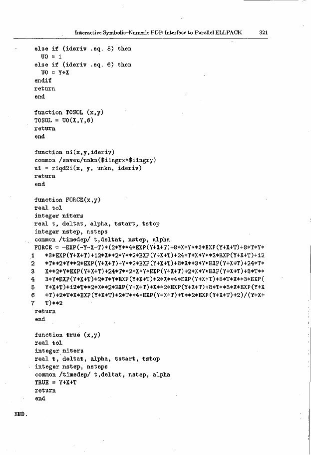
Appendix:/ /ELLPACK program template for solving (2.13)
OPTIONS. 11time = .true. clockwise = .true. xplot3d
DECLARATIONS. real tol integer niters common /saveu/ unkn($i1ngrx,$i1ngry)
GLOBAL. real t, deltat, alpha, tstart, tstop integer nstep, nsteps common Jtimedep/ t,deltat, nstep, alpha
EQUATION. ALPHA*EXP(-U(X,Y))/U(X,Y)**2*UXX+ALPHA*EXP(-U(X,Y))/U(X,Y)**2*UYY+ &
ALPHA*(-2*EXP(-U(X,Y))*UX(X,Y)/U(X,Y)**2-U(X,Y)**2)*UX+ALPHA*(- & 2*EXP(-U(X,Y))*UY(X,Y)/U(X,Y)**2-U(X,Y)**2)*UY+(ALPHA*(-2*(EXP( & -U(X,Y))*UYY(X,Y)-EXP(-U(X,Y))*UY(X,Y)**2)/U(X,Y)**3+(EXP(-U(X, & Y))*UY(X,Y)**2-EXP(-U(X,Y))*UYY(X,Y))/U(X,Y)**2-2*U(X,Y)*UY(X,Y & )-2*(EXP(-U(X,Y))*UXX(X,Y)-EXP(-U(X,Y))*UX(X,Y)**2)/U(X,Y)**3+( & EXP(-U(X,Y))*UX(X,Y)**2-EXP(-U(X,Y))*UXX(X,Y))/U(X,Y)**2-2*U(X, & Y)*UX(X,Y))-1/DELTAT)*U = EXP(-U(X,Y))*((-ALPHA*U(X,Y)-2*ALPHA) & *UYY(X,Y)+(ALPHA*U(X,Y)+ALPHA)*UY(X,Y)**2-2*ALPHA*U(X,Y)**4*EXP & (U(X,Y))*UY(X,Y)+(-ALPHA*U(X,Y)-2*ALPHA)*UXX(X,Y)+(ALPHA*U(X,Y) & +ALPHA)*UX(X,Y)**2-2*ALPHA*U(X,Y)**4*EXP(U(X,Y))*UX(X,Y)+PDERS( & X,Y)*U(X,Y)**2*EXP(U(X,Y))+ALPHA*FORCE(X,Y)*U(X,Y)**2*EXP(U(X,Y & )))/U(X,Y)**2
BOUNDARY.
GRID.
u=true(x,y) on x=O u=true(x,y) on x=1 u=true(x,y) on y=O u=true(x,y) on y=1
10 x points 10 y points
TRIPLE. set (u = tOsol)
FORTRAN. call save (ritabl, i1ngrx*i1ngry)
Interactive Symbolic-Numeric PDE Interface to Parallel ELLPACK
11cstc = .false. alpha= 0.5 tstart = 0.0 tstop = 5.0 deltat = 0.1 nsteps = int ((tstop-tstart)/deltat + 0.5) deltat = (tstop - tstart)/nsteps
do 100 nstep = 1, nsteps t = tstart + nstep*deltat
TRIPLE. set u by blending
FORTRAN. niters = 10 · tol = 0.005 do 300 i = 1, niters print *• 'time=',t,' ·,iteration=·', i
DISCRETIZATION. 5 point star
INDEXING. as is
SOLUTION. band ge
OUTPUT. max (error)
FORTRAN. i1levl = 0
* test for convergence if (R1NRMI .lt. tol) then
go to 301 endif
300 continue print *• 'failed to converge!' go to 302
301 continue print *• 'converged in', i, ' iterations.'
302 continue
FORTRAN.
319
320 S. Weerawarana, E.N. Houstis and J.R. Rice
call q35pvl call save (r1tabl, i1ngrx*i1ngry)
100 continue
SUBPROGRAMS. +both.
subroutine save (arr, len) real arr(1) common /saveu/ unkn($i1ngrx*$i1ngry) do 101 i = 1,len
unkn(i) = arr(i) 101 continue
return end
function PDERS(x,y) real t, deltat, alpha, tstart, tstop external u1 integer nstep, nsteps common /timedep/ t,deltat, nstep, alpha t = t - deltat if (nstep .eq. 1) then
PDERS = (ALPHA-1.0)*(-UO(X,Y,5)*UO(X,Y,6)**2-UO(X,Y,4)*UO(X,Y,6) 1 **2+(UO(X,Y,3)*EXP(-UO(X,Y,6))-UO(X,Y,5)**2*EXP(-UO(X,Y,6)))/ 2 UO(X,Y,6)**2+(UO(X,Y,1)*EXP(-UO(X,Y,6))-UO(X,Y,4)**2*EXP(-UO( 3 X,Y,6)))/UO(X,Y,6)**2-FORCE(X,Y))-UO(X,Y,6)/DELTAT else
PDERS = (ALPHA-1.0)*((EXP(-U1(X,Y,6))*U1(X,Y,3)-EXP(-U1(X,Y,6))* 1 U1(X,Y,5)**2)/U1(X,Y,6)**2-U1(X,Y,6)**2*U1(X,Y,5)+(EXP(-U1(X, 2 Y,6))*U1(X,Y,1)-EXP(-U1(X,Y,6))*U1(X,Y,4)**2)/U1(X,Y,6)**2-U1 3 (X,Y,6)**2*U1(X,Y,4)-FORCE(X,Y))-U1(X,Y,6)/DELTAT
end if t = t + deltat return end
function UO(x,y,ideriv) real t, deltat, alpha, tstart, tstop integer nstep, nsteps common /timedep/ t,deltat, nstep, alpha if (ideriv .eq. 1) then
uo = 0 else if (ideriv .eq. 2) then
uo = 0 else if (ideriv .eq. 3) then
uo = 0 else if (ideriv .eq. 4) then
uo = 1 I
J
END.
Interactive Symbolic-Numeric PDE Interface to Parallel ELLPACK 321
else if (ideriv .eq. 6) then uo = 1
else if (ideriv .eq. 6) then UO = Y+X
endif return end
function TOSOL (x,y) TOSOL = UO(X,Y,6) return end
function ui(x,y,ideriv) common /saveu/unkn($i1ngrx*$i1ngry) u1 = r1qd2i(x, y, unkn, ideriv) return end
function FORCE(x,y) real tol integer niters real t, deltat, alpha, tstart, tstop integer nstep, nsteps common /timedep/ t,deltat, nstep, alpha FORCE = -EXP(-Y-X-T)*(2*Y**4*EXP(Y+X+T)+8*X*Y**3*EXP(Y+X+T)+8*T*Y*
1 *3*EXP(Y+X+T)+12*X**2*Y**2*EXP(Y+X+T)+24*T*X*Y**2*EXP(Y+X+T)+12 2 *T**2*Y**2*EXP(Y+X+T)+Y**2*EXP(Y+X+T)+8*X**3*Y*EXP(Y+X+T)+24*T* 3 X**2*Y*EXP(Y+X+T)+24*T**2*X*Y*EXP(Y+X+T)+2*X*Y*EXP(Y+X+T)+8*T** 4 3*Y*EXP(Y+X+T)+2*T*Y*EXP(Y+X+T)+2*X**4*EXP(Y+X+T)+8*T*X**3*EXP( 6 Y+X+T)+12*T**2*X**2*EXP(Y+X+T)+X**2*EXP(Y+X+T)+8*T**3*X*EXP(Y+X 6 +T)+2*T*X*EXP(Y+X+T)+2*T**4*EXP(Y+X+T)+T**2*EXP(Y+X+T)+2)/(Y+X+ 7 T)**2 return end
function true (x,y) real tol integer niters real t, deltat, alpha, tstart, tstop integer nstep, nsteps common /timedep/ t,deltat, nstep, alpha TRUE = Y+X+T return end