switching asymmetric garch and options on a volatility index

SWITCHING ASYMMETRIC

GARCH AND OPTIONS

ON A VOLATILITY INDEX

HAZEM DAOUK*JIE QUN GUO

Few proposed types of derivative securities have attracted as much atten-tion and interest as option contracts on volatility. Grunbichler andLongstaff (1996) is the only study that proposes a model to value optionswritten on a volatility index. Their model, which is based on modelingvolatility as a GARCH process, does not take into account the switchingregime and asymmetry properties of volatility. We show that theGrunbichler and Longstaff (1996) model underprices a three-monthoption by about 10%. A Switching Regime Asymmetric GARCH is used tomodel the generating process of security returns. The comparison betweenthe switching regime model and the traditional uni-regime model amongGARCH, EGARCH, and GJR-GARCH demonstrates that a switchingregime EGARCH model fits the data best. Next, the values of Europeancall options written on a volatility index are computed using Monte Carlointegration. When comparing the values of the option based on theSwitching Regime Asymmetric GARCH model and the traditional

Our thanks go to Timothy Crack, Partha Deb, Craig Holden, Michael Sullivan, George Wang,Robert Webb (the editor), two anonymous referees, and participants at the 2000 FinancialManagement Association meeting for helpful discussions and comments. Opinions of the authorsare not necessarily those of Fannie Mae. Remaining errors are our own.*Correspondence author, Cornell University, Department of Applied Economics & Management,446 Warren Hall, Ithaca, NY 14853 USA; e-mail: [email protected]

Received March 2000; Accepted March 2003

� Hazem Daouk is an Assistant Professor at Cornell University, Department of AppliedEconomics & Management, Ithaca, New York.

� Jie Qun Guo is an Economist at Fannie Mae, Washington DC.

The Journal of Futures Markets, Vol. 24, No. 3, 251–282 (2004) © 2004 Wiley Periodicals, Inc.Published online in Wiley InterScience (www.interscience.wiley.com). DOI: 10.1002/fut.10114

252 Daouk and Guo

GARCH specification, it is found that the option values obtained from thedifferent processes are very different. This clearly shows that theGrunbichler-Longstaff model is too stylized to be used in pricing deriva-tives on a volatility index. © 2004 Wiley Periodicals, Inc. Jrl Fut Mark24:251–282, 2004

INTRODUCTION

Few proposed types of derivative securities have attracted as much atten-tion and interest as option contracts on volatility. The objective of thispaper is to show that pricing options on a volatility index demandsextreme care in modeling the underlying process. Grunbichler andLongstaff (1996), or G-L, is the only paper that proposes a model tovalue options on a volatility index. Their model is based on a GARCHspecification for the underlying asset. It is argued that the GARCH spec-ification leads to severe mispricing in the option value because it doesnot allow for regime switching and volatility asymmetry (leverage effect).No volatility options data is available, since those derivatives are nottraded yet. Hence, we cannot use real prices to test the option pricingmodels. For that reason, we use simulation to obtain our results.Nevertheless, it is argued that it is more useful to explore and test optionpricing models before the derivatives are introduced and traded, ratherthan after they are already priced in the market.

Ever since Mandelbrot (1963) suggested that large changes tend tobe followed by large changes—of either sign—and small changes tend tobe followed by small changes, a number of papers have illustrated thatstock variance exhibits temporal dependence (for example, Akgiray,1989). To capture this feature, Engle (1982) develops a new class of sto-chastic processes, the AutoRegressive Conditional Heteroscedasticity(ARCH) models, in which the conditional variance is a function of pastresiduals. It has been shown that allowing the conditional variance to betime-varying generates fat tails for the distribution of returns. Bollerslev(1986) introduces the Generalized ARCH (GARCH) which extendsEngle’s ARCH by allowing the conditional variance to be a function ofthe lagged variance. Bollerslev (1986) shows that the GARCH modelallows a better representation of the volatility process while being moreparsimonious.

Another important stylized fact of stock returns is that their volatili-ty tends to rise in response to “bad news” (excess returns lower thanexpected) and fall in response to “good news” (excess returns higher thanexpected). This is also known in the literature under the name of“volatility asymmetry” or “leverage effect,” since leverage provides at

Options on a Volatility Index 253

least a partial explanation. As the price of a stock decreases, the firmleverage will increase, assuming that debt value did not decrease by asmuch. Since the volatility of equity is an increasing function of leverage,this provides a simple explanation for asymmetry (Black, 1976). Anotherexplanation was given by French, Schwert, and Stambaugh (1987). Theyargue that the negative relation between volatility and stock prices is dueto the fact that an increase in unexpected volatility will increase theexpected future volatility (assuming persistence). Then, the risk premi-um will also increase causing prices to drop. Nelson (1991) introducesthe EGARCH model (Exponential GARCH) to account for volatilityasymmetry. Also, Glosten, Jagannathan, and Runkle (1993) introduce analternative specification know as the GJR-GARCH (see Bollerslev et al.,1992, for an extensive review of the literature).

Recently, Cai (1994) and Hamilton and Susmel (1994) introducethe Markov-Switching Regime ARCH (SWARCH) model that incorpo-rates the features of both Hamilton’s (1988, 1989) switching regimemodel and Engle’s ARCH model. Hamilton’s switching regime model canbe described as an autoregressive process in which the parameters of theautoregression can change as the result of a regime-shift variable. Theregime itself will be described as the outcome of an unobserved Markovchain. The basic idea is to allow the data generating process to bedifferent in different regimes. The existence of multiple regimes is apervasive phenomenon in financial economics. More recently, switching-regime models have been applied to stock market returns (Norden &Schaller, 1993), foreign stock markets (Bollen et al., 2000; Norden,1995; Rockinger, 1994), and interest rates (Ang & Bekaert, 1998;Dahlquist & Gray, 2000; Gray, 1996a, 1996b).

In this paper, we extend the SWARCH model to a Markov SwitchingRegime Asymmetric GARCH (SW-Asymmetric GARCH). The SW-Asymmetric GARCH allows both regime switching in volatility andasymmetry. It is argued that the additional effort required in estimatingthe model is justified by the benefit of providing a richer modeling of thevolatility dynamics.

The remainder of this paper is organized as follows. The next sec-tion describes volatility indices and options written on volatility indices.The following section presents a brief exposition of the Grunbichler andLongstaff (1996) model, and shows that the assumed process for volatil-ity is a continuous time limit of a GARCH model. Next we present thegeneral methodology used in assessing if the volatility process in G-L isappropriate. The next section provides detailed discussion of the switch-ing regime model and the model selection criteria. The following section

254 Daouk and Guo

1Eight near-the-money, nearby, and second nearby OEX call and put options provide the inputs forconstructing the volatility index. First, the implied volatilities of the call and the put in each of thefour categories of options are averaged. Second, at-the-money implied volatilities are created byinterpolating between the nearby and second nearby average implied volatilities. In this way, VIX isalways at-the-money. Finally, a constant time to expiration is maintained. The nearby and secondnearby at-the-money volatilities are weighted to create a constant 30-calendar day (22-trading day)time to expiration.2Brenner and Galai (1989) and Whaley (1993) provide excellent discussions of how volatility deriv-atives can be used to hedge the volatility risk of portfolios containing options or securities withoption-like features. See also Fleming, Ostdiek, and Whaley (1995) and Whaley (2000) for a thor-ough analysis of VIX.

contains results from fitting the volatility models, and rejects theGARCH specification in favor of those allowing for switching regime andasymmetry. Next we show that option prices computed with the G-Lassumed process underprice volatility index options by a considerableamount. Then, we provide further analysis and robustness checks. Thefinal section concludes.

OPTIONS ON A VOLATILITY INDEX

Few proposed types of derivative securities have attracted as much atten-tion and interest as option contracts on volatility. Grunbichler andLongstaff (1996) cite various sources including Reuters, The Wall StreetJournal, Futures, Futures and Options World, Barrons, etc., that discussthose derivatives. The underlying asset for those options is the MarketVolatility Index (VIX). VIX is an average of S&P 100 option (OEX)implied volatilities. It was introduced by the Chicago Board OptionsExchange (CBOE) to provide an up-to-the-minute measure of expectedvolatility of the US equity market.1 According to Duke Chapman, CBOEformer chairman, the index is particularly suited for institutionalinvestors interested in hedging future, not past changes in portfolio risk(see Vosti, 1993). Robert Whaley, the developer of the index, declaredthat the availability of an option contract on the CBOE Market VolatilityIndex will allow market participants to manage the risks associated withunanticipated changes in volatility.2 The CBOE has applied to theSecurities and Exchange Commission to trade European options on thevolatility index. Yet, this operation was constantly delayed. The reason forthat seems to be that market makers are still trying to understand theimplications and risks involved in trading volatility derivatives. Morerecently, many European exchanges have introduced volatility indices inthe hope of trading volatility derivatives (two examples are the VX1 andVX6 volatility indices from MONEP in France and the VLEU volatilityindex in Switzerland). Some exchanges have even started to trade futures


on volatility indices (VOLAX futures from the Deutsche Terminborse inGermany, SEK volatility futures for the Swedish market, and FTSEvolatility futures in the United Kingdom). A better understanding ofvolatility options, and the way they should be priced, will facilitate theintroduction and adoption of volatility options worldwide. This papercontributes in this direction.

THE GRUNBICHLER AND LONGSTAFF (1996)MODEL

Grunbichler and Longstaff (1996), or G-L, is the only paper to ourknowledge that presents a model to price options on a volatility index.The major assumption of their model is that related to the specificationof the dynamics of the underlying process, i.e., volatility. The volatilityindex, denoted V, is modeled as a mean reverting process

(1)

where v, k, and s are constants, and Z is a standard Wiener process.Since V is not the price of a traded asset, it is assumed that the

expected premium for volatility risk is proportional to the level of volatil-ity, zV where z is a constant parameter.

The G-L model captures many of the observed properties of volatil-ity. In particular, the model allows volatility to be mean reverting andconditionally heteroscedastic.

We argue below that the G-L specification for volatility is indeed thecontinuous time limit of a GARCH model. Nelson (1990) investigatesthe convergence of stochastic difference equations for volatility models tostochastic differential equations as the length of the discrete time intervalsbetween observations goes to zero. We present the results from Nelson’s(1990) derivation of the continuous time limits of a GARCH(1,1) in ourown notation.

A GARCH(1,1) model can be written as follows:

(2)

where

ht is conditional volatility, and a1, d1, and g are constant parameters.

zt i.i.d. � N(0, 1)

et � h1�2t zt

ht � a � d1ht�1 � ge2t�1

dV � (v � kV) dt � s1V dZ

256 Daouk and Guo

3The options we are interested in are written on a volatility index implied from options. The volatilityprocesses we simulate to compute the option prices represent the instantaneous (or a discreteapproximation to the instantaneous) volatility of the S&P 100 index. As Grunbichler and Longstaff(1996) note, the volatility can be either the instantaneous volatility or the volatility implied fromsome option pricing model—the distinction does not affect the form of the resulting valuation pro-cedure. For example, Taylor and Xu (1994) show that when volatility is stochastic, the volatility esti-mate implied by inverting the Black-Scholes model is nearly a linear function of the actual instanta-neous volatility.

Nelson (1990) derives diffusion limits of the form

(3)

where w, �, and q are constant parameters, and Z is a standard Wienerprocess.

As can be seen, the derived model in (3) is essentially the G-L spec-ification. In fact, GARCH models do imply mean reversion in volatility(the coefficients need to sum to less than one for stationarity) and con-ditional heteroskedasticity (the change in conditional volatility is largerfor larger levels of volatility).

IS THE GRUNBICHLER AND LONGSTAFF(1996) VOLATILITY PROCESS APPROPRIATE?

The GARCH specification for the volatility process suffers from twomajor drawbacks. The first one is that it does not allow for volatilityasymmetry (leverage effect). The second drawback is that it does notaccount for regime switching (regime shifts). The objective of this paperis not to criticize the specific form of the volatility model in G-L. Rather,we want to show that any model not accounting for the switching regimeand asymmetry properties will severely misprice (undervalue) volatilityoptions. To that end, we compare option prices computed using a simpleGARCH process to those computed using switching and asymmetricmodels.3

In the literature, many studies have derived closed form solutionsfor stock options with stochastic volatility (Heston, 1993; Hull & White,1987; Stein & Stein, 1991). Those models came in response to theempirical evidence related to time-varying volatility. Also, stock optionpricing models where stock volatility follows a GARCH process havebeen derived by Duan (1995) and Heston and Nandi (1999). Morerecently, studies like Ritchey (1990), Billio and Pelizzon (1996), Bollen(1998), Duan, Popova, and Ritchken (1999), and Campbell and Li(1999) develop models obtained when the stock dynamic is modeled by aMarkov regime-switching process. The regimes are characterized bydifferent volatility levels. Those models differ from the previous ones in

dh � (w � �h) dt � qh dZ


4Also, Walsh (1999) examines the effect of ignoring conditional volatility on the price of stockoptions. He considers many GARCH models including asymmetric ones. He finds that asymmetricGARCH effects exacerbate the bias in the price of the options.

that rather than permitting volatilities to follow a continuous time, con-tinuous state process, their focus is on cases where volatilities can takeon a finite set of values, and can only switch regimes at finite times.There is still very little work on volatility asymmetry as applied to optionpricing. Along those lines, Schobel and Zhou (1998) use Fourier inver-sion techniques to price stock options allowing for correlation betweeninstantaneous volatilities and the underlying stock returns. This is a firststep towards accounting for volatility asymmetry.4

Many of the above studies are able to show that their model presentan improvement over Black and Scholes (1973) that is statistically sig-nificant. However, this improvement is not economically large. On theother hand, in our case, the model in Grunbichler and Longstaff (1996)will be shown to misprice option on volatility by a very large amount.There are reasons to believe that mispecifying the volatility process whenthe option is written on a stock index is much less serious than in thecase where the option is written on a volatility index. In the first case,the volatility process is a major determinant of the underlying assetprocess. In the second case, the volatility process is the underlying asset.Ignoring regime switching in the volatility process might not be too badof an approximation when pricing derivatives on a stock index, as long asvolatility is allowed to be stochastic. However, It is argued that ignoringregime switching and asymmetry in volatility when pricing derivatives ona volatility index could be disastrous.

None of the above models can be used to price options on volatility.The only model that can do that is that of G-L. Their model assumes thatvolatility follows a stochastic process that is the continuous time ana-logue of GARCH. As argued before, this process does not allow volatilityasymmetry. Also, it does not allow the parameters of the autoregressiveprocess to be different for different regimes. We note that this is a short-coming that is common to all the option models reviewed above. Giventhe large empirical evidence related to volatility asymmetry and regimeswitching, there are reasons to suspect that volatility options pricedunder the GARCH or other “simple” stochastic volatility assumptionswill be significantly mispriced. It will be demonstrated that the mispric-ing in the case of options on a volatility index is very large economically.

There are no analytic solutions for the price of options on a volatilityindex under the assumption of volatility following a switching asymmet-ric autoregressive process. Therefore, Monte Carlo integration is used tocompute the option values. Also option values for the G-L model are

258 Daouk and Guo

computed using Monte Carlo integration instead of using analyticsolutions. There are two reasons for that choice.

First, we want to conduct hypothesis testing from fitting the differ-ent processes to the S&P 100 data. By using a GARCH process for theG-L model, we are able to compare its fit to the data with that of othermore rich volatility processes. As will be shown in the next section, theGARCH model can be nested in the switching asymmetric GARCHmodels, allowing for hypothesis testing for nested models (likelihoodratio). This will allow us to test the hypothesis that the GARCH processis an adequate representation of the data as compared to the moregeneral processes.

The second reason why option prices for the G-L model are com-puted using Monte Carlo integration is that the GARCH specification iswidely used in the literature and has been found to be flexible enough tofit the data well. The point is that using the simple GARCH impliesaccepting the restrictive assumptions of no switching or asymmetricproperties in volatility. Those assumptions might be convenient to workwith in some contexts. However, we want to show that those assump-tions are not appropriate to use to price options on volatility.

SWITCHING REGIME ASYMMETRIC GARCH MODELS

Model Specification

The Switching Regime Asymmetric GARCH models used in this paperare part of the family of Markov switching regime models (see chapter 22of Hamilton, 1994). A common finding using high-frequency financialdata concerns the apparent persistence implied by the estimates for theconditional variance functions. This has prompted Bollerslev and Engle(1986) to introduce the class of integrated GARCH or IGARCH.However, the intuitive appeal and fit of this model has raised questions.Cai (1994) and Hamilton and Susmel (1994) have addressed the issueby proposing Markov switching volatility models. They note that the per-sistence implied by the model in Bollerslev and Engle (1986) is difficultto reconcile with the poor forecasting performance. Further, it is arguedthat the poor forecasting performance and spuriously high persistencemight be related to structural change in the volatility process. This isrelated to Perron’s (1989) observation that changes in regime may givethe spurious impression of unit roots in characterizations of the level ofa series. For example, Cai (1994) and Hamilton and Susmel (1994) findthat volatility of returns appears to be much less persistent when one


models changes in the parameter through a Markov switching process.The SWARCH model allows occasional shifts in the asymptotic varianceof the ARCH process by having the intercept term switch between dif-ferent values depending on what volatility regime the process is in. Thetraditional ARCH-type models rely on the assumption of parametrichomogeneity. This means that the parameters of the model remain thesame whether the market is in a calm regime or a volatile regime. Whatdistinguishes periods of high volatility from periods of low volatility is thesize of the residual. On the other hand, the SWARCH model allows therelation between the conditional volatility and the explanatory variables(lagged residuals) to be different between periods of high volatility andperiods of low volatility. Kim and Kon (1999) provide evidence that thetime-series properties of stock returns include both structural changeand time dependence in the conditional variance. The estimation of aSWARCH model determines the parameters of the ARCH terms (whichinclude different parameters for different regimes) along with transitionprobabilities between the different regimes. Cai (1994) and Hamiltonand Susmel (1994) show that their model is better able to capture thebehavior of returns volatility than previous ARCH-type models. Sincethen, the SWARCH model has been applied to international equity mar-kets (Fornari & Mele, 1997; Susmel, 1994, 1998a), and inflation timeseries (Susmel, 1998b). We follow Cai (1994) and Hamilton and Susmel(1994) in adopting a Markov switching regime model. We believe thatthis will account for volatility persistence in an appropriate manner. Cai(1994) and Hamilton and Susmel (1994) propose and estimate aSwitching-ARCH. The dynamic lag structure, was restricted to an ARCHspecification. This is a drawback since the GARCH specification hasbeen shown to be a better fit to financial data. We generalize theSWARCH model to a GARCH specification. We are able to account forvolatility asymmetry by using an Asymmetric GARCH. Furthermore, weallow the persistence of volatility and the asymmetry to be differentbetween different regimes. This means that when there is a change inthe regime, the model that is used to generate conditional volatility isreplaced by a different model with different parameters.

Formally, let Rt be a vector of observed variables and let st denote anunobserved random variable that can take on the values Suppose that st can be described by a Markov chain

(4)� Prob(st � j 0 st�1 � i) � pij

Prob(st � j 0 st�1 � i, st�2 � k, . . . , �t)

1, 2, . . . , C.

260 Daouk and Guo

for It is sometimes convenient to collect the transitionprobabilities in a (C � C) matrix:

(5)

Note that each column of sums to unity.A useful representation for a Markov chain is obtained by letting jt

denote a random (C � 1) vector whose jth element is equal to unity ifst � j and whose jth element equals zero otherwise:

(6)

The variable st is regarded as the state or regime that the process isin at date t. By this, we mean that st governs that parameters of the con-ditional distribution of Rt. The density of Rt is conditional on its ownlagged values as well as on the current and previous q values for the stateis of the form

The methods developed in Hamilton (1989) are used to evaluate thelikelihood function for the observed data and make inferences about theunobserved regimes. In this case, the returns Rt follow a process inthe ARCH family whose parameters depend on the unobserved realiza-tion of The objective is to select a parsimonious repre-sentation for the different possible regimes.

For a two-regime switching model, C is equal to 2. In other words,the volatility of security returns are assumed to be generated from tworegimes which are different in describing the underlying behavior.

Bera and Higgins (1993) find that with a parametric specification ofthe conditional variance function, there does not appear to be a densityfunction that is suitable for all security data. It is of interest to see if after

st, st�1, . . . , st�q.

f(Rt 0 st, st�1, . . . , st�q, �t)

jt � h

(1, 0, 0, . . , 0)��when st � 1(0, 1, 0, . . , 0)��when st � 2::

(0, 0, 0, . . , 1)��when st � C

�

q � ≥ p11 p21 . . pC1

p12 p22 . . pC2

: : . . :

p1C p2C . . pCC

¥i, j � 1, 2, . . . , C.


5One of the benefits of the normality assumption is that the parameter estimates are asymptoticallyunbiased, even if the true distribution is non-normal, provided the first two conditional moments arecorrectly specified (Weiss, 1986). On the other hand, the t distribution does not have this robustproperty.

allowing for regime switching, a normal distribution for Rt will be ade-quate in fitting the data.5

Since we focus on the influence of volatility on the price of options,we use the simplest specification for the mean equation

(7)

where . We use different specifications forthe conditional variance equation.

For GARCH(1,1),

(8)

For EGARCH(1,1),

(9)

For GJR-GARCH(1,1),

(10)

where and 0 otherwise.As can be seen, ht is a function of That is, the conditional vari-

ance is time dependent and relies on past information. The (1,1) formu-lation (p � q � 1) is used because it has consistently been found tomodel variance dynamics adequately (e.g., Akgiray, 1989; Bollerslev,1986). Moreover, a natural specification is needed to avoid overfittingthe data. The focus is on highlighting the switching and asymmetryproperties of the data. The EGARCH and GJR-GARCH specificationsallow for volatility asymmetry (leverage effect). If there exists volatilityasymmetry consistent with previous literature, then we should find thatg2 � 0 in EGARCH(1,1) and g2 0 in GJR-GARCH(1,1).

Model Estimation and Selection

The switching regime model is based on the discrete heterogeneityassumption. The volatility of security returns has been shown to be per-sistent. However, this relationship behaves differently between different

�t.St � 1 if et�1 � 0

ht � a � d1ht�1 � g1e2t�1 � g2St�1e

2t�1

ln(ht) � a � d1ht�1 � g1 0zt�1 0 � g2zt�1

ht � a � d1ht�1 � ge2t�1

et � h1�2t zt, zt i.i.d. � N(0, 1)

Rt � m � et

262 Daouk and Guo

6The switching regime model is considered to be semi-parametric because knowledge of the distri-bution of the unobserved mixing variable is not required. Hence, we need not know which factorsdetermine , the matrix of transition probabilities.7However, we are comfortable with that choice because in an earlier version of this paper, we com-pared a more restrictive version of our model (i.i.d. mixtures) with three regimes and two regimesrespectively. We found that the model with two regimes was a better fit to the data.

�

regimes (see Cai, 1994). The underlying reasons that causes this differentbehavior are unobservable but are highly related to regime conditions.Our model is able to classify heterogeneity into a small finite number ofrelatively homogeneous regimes (a calm regime and a volatile regime).6

One of the difficulties in using switching regime models is decidingon how many regimes are needed in the model. In practice, one can startwith a small number of regimes and add more provided the fit of themodel is significantly improved. In this paper, we use a two-regime-switching model because of the extreme difficulty in estimating a modelwith a larger number of regimes.7

Let denote all unknown parameters, . Let T bethe sample size. Let Prob( denote the inference about thevalue of st based on data obtained through date t and based on a “guess”of the population parameters (starting values). Collect these condi-tional probabilities Prob( for in a (C � 1)vector denoted

Also, forecasts of how likely the process is to be in regime j in periodt � 1 are formed given observations obtained through date t. These fore-casts are collected in a (C � 1) vector which is a vector whose jthelement represents Prob(

The optimal inference and forecast for each date t in the sample canbe found by iterating on the following pair of equations:

(11)

(12)

Here 1� represents a (1 � C) vector of 1s, and the symbol denoteselement-by-element multiplication. Given a starting value and anassumed value for the population parameter vector , one can iterate onthe above two equations for to calculate the values of and for each date t in the sample. The log-likelihood function for the observed data evaluated at the value of that was used to per-form the iterations can also be calculated as a by-product of this

U�T

L(U)jt�1 0 t jt 0 tt � 1, 2, . . . , TU

j1 0 0�

jt 0 t�1 � q jt 0 t jt 0 t �

(jt 0 t�1 � ht)

1�(jt 0 t�1 � ht)

st�1 � j 0 �t; U).jt�1 0 t,

jt 0 t. j � 1, 2, . . . , Cst � j 0 �t; U)U

st � j 0 �t; U)U � (�, m, d, g)U


8Sometimes, the conclusions drawn from AIC and BIC are not the same. This can happen becauseBIC is more severe in penalizing non-parsimonious specifications than AIC.

algorithm from

(13)

where

(14)

Robust standard errors are computed to account for heteroscedas-ticity and serial correlation. The likelihood ratio (LR) test, penalized AICand BIC are used as selection vehicles to compare models.

The LR test is a popular test for multiple parameter situations (seeKon, 1984). The following models were tested against each others:GARCH, Switching Variance, GJR-GARCH, EGARCH, SW-GARCH,SW-GJR-GARCH, and SW-EGARCH.

The model corresponding to the null hypothesis (H0) is nested withinthe model corresponding to the alternative (H1). If H0 is true,

(15)

has an asymptotic chi-square distribution with degrees of freedom equal top (the difference in the number of parameters between H0 and H1).However, the method may not be appropriate for the switching modelbecause the hypothesis is on the boundary of the parameter space and thisviolates the standard regularity condition for maximum likelihood.Böhning et al. (1994) show that using LR test is likely to underreject thefalse null when the boundary condition is involved. Hence, the test tendsto choose a small number of components. As alternative methods, we usepenalized Akaiki Information Criterion (AIC � �2L(u) � 2K) and BaysianInformation Criterion (BIC � �2L(u) � K ln(N)). These methods arerobust in a sense that they are valid even when the model is misspecified.The model with the lowest value of AIC or BIC is considered the best.8

ESTIMATION RESULTS ANDHYPOTHESES TESTING

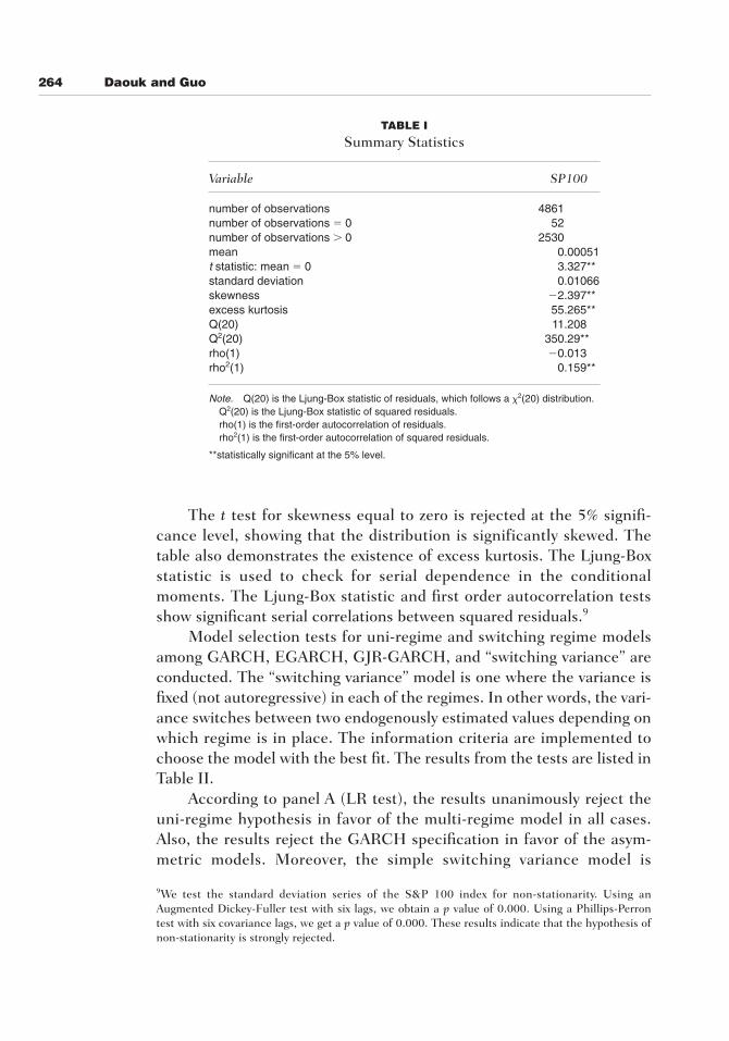
We use daily continuously compounded S&P 100 index (SP100) returnsfrom the period January 3, 1980 to March 26, 1999. Summary statisticsare reported in Table I.

�2L(u) � �2[L(uH0) � L(uH1

)]

f(Rt 0 �t�1; U) � 1�(jt 0 t�1 � ht)

L(U) � aT

t�1log f(Rt 0 �t�1; U)

264 Daouk and Guo

TABLE I

Summary Statistics

Variable SP100

number of observations 4861number of observations � 0 52number of observations 0 2530mean 0.00051t statistic: mean � 0 3.327**standard deviation 0.01066skewness �2.397**excess kurtosis 55.265**Q(20) 11.208Q2(20) 350.29**rho(1) �0.013rho2(1) 0.159**

Note. Q(20) is the Ljung-Box statistic of residuals, which follows a �2(20) distribution.Q2(20) is the Ljung-Box statistic of squared residuals.rho(1) is the first-order autocorrelation of residuals.rho2(1) is the first-order autocorrelation of squared residuals.

**statistically significant at the 5% level.

9We test the standard deviation series of the S&P 100 index for non-stationarity. Using anAugmented Dickey-Fuller test with six lags, we obtain a p value of 0.000. Using a Phillips-Perrontest with six covariance lags, we get a p value of 0.000. These results indicate that the hypothesis ofnon-stationarity is strongly rejected.

The t test for skewness equal to zero is rejected at the 5% signifi-cance level, showing that the distribution is significantly skewed. Thetable also demonstrates the existence of excess kurtosis. The Ljung-Boxstatistic is used to check for serial dependence in the conditionalmoments. The Ljung-Box statistic and first order autocorrelation testsshow significant serial correlations between squared residuals.9

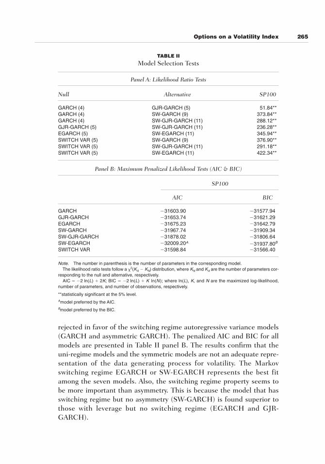
Model selection tests for uni-regime and switching regime modelsamong GARCH, EGARCH, GJR-GARCH, and “switching variance” areconducted. The “switching variance” model is one where the variance isfixed (not autoregressive) in each of the regimes. In other words, the vari-ance switches between two endogenously estimated values depending onwhich regime is in place. The information criteria are implemented tochoose the model with the best fit. The results from the tests are listed inTable II.

According to panel A (LR test), the results unanimously reject theuni-regime hypothesis in favor of the multi-regime model in all cases.Also, the results reject the GARCH specification in favor of the asym-metric models. Moreover, the simple switching variance model is


TABLE II

Model Selection Tests

Panel A: Likelihood Ratio Tests

Null Alternative SP100

GARCH (4) GJR-GARCH (5) 51.84**GARCH (4) SW-GARCH (9) 373.84**GARCH (4) SW-GJR-GARCH (11) 288.12**GJR-GARCH (5) SW-GJR-GARCH (11) 236.28**EGARCH (5) SW-EGARCH (11) 345.94**SWITCH VAR (5) SW-GARCH (9) 376.90**SWITCH VAR (5) SW-GJR-GARCH (11) 291.18**SWITCH VAR (5) SW-EGARCH (11) 422.34**

Panel B: Maximum Penalized Likelihood Tests (AIC & BIC)

SP100

AIC BIC

GARCH �31603.90 �31577.94GJR-GARCH �31653.74 �31621.29EGARCH �31675.23 �31642.79SW-GARCH �31967.74 �31909.34SW-GJR-GARCH �31878.02 �31806.64SW-EGARCH �32009.20A �31937.80B

SWITCH VAR �31598.84 �31566.40

Note. The number in parenthesis is the number of parameters in the corresponding model.The likelihood ratio tests follow a �2(KA � KN) distribution, where KN and KA are the number of parameters cor-

responding to the null and alternative, respectively.AIC � �2 ln(L) � 2K; BIC � �2 ln(L) � K ln(N ); where ln(L), K, and N are the maximized log-likelihood,

number of parameters, and number of observations, respectively.

**statistically significant at the 5% level.Amodel preferred by the AIC.Bmodel preferred by the BIC.

rejected in favor of the switching regime autoregressive variance models(GARCH and asymmetric GARCH). The penalized AIC and BIC for allmodels are presented in Table II panel B. The results confirm that theuni-regime models and the symmetric models are not an adequate repre-sentation of the data generating process for volatility. The Markovswitching regime EGARCH or SW-EGARCH represents the best fitamong the seven models. Also, the switching regime property seems tobe more important than asymmetry. This is because the model that hasswitching regime but no asymmetry (SW-GARCH) is found superior tothose with leverage but no switching regime (EGARCH and GJR-GARCH).

266 Daouk and Guo

TABLE III

Parameter Estimates of SW-EGARCH

SP100

Variable Regime 1 Regime 2

a �0.1267** �0.3376(0.0203) (0.7453)

d1 0.9928** 0.9676**(0.0018) (0.0785)

g1 0.0695** 0.2670(0.0126) (0.3753)

g2 �0.0197** �0.3113(0.0100) (0.2070)

m 0.0005**(0.0001)

p11 0.9675**(0.0393)

p22 0.2675(0.2513)

log-likelihood 16015.585Q(20) 20.916Q2(20) 7.953rho(1) 0.0138rho2(1) �0.0133skewness �0.4158**excess kurtosis 3.6155**

Note. The EGARCH(1,1) specification is defined as follows

where ht is the conditional variance, zt i.i.d. ~ N(0, 1), and �, �1, �1, and �2 are constantparameters.

The numbers in parenthesis are standard errors.

Q(20) is the Ljung-Box statistic of residuals, which follows a x2(20) distribution.Q2(20) is the Ljung-Box statistic of squared residuals.rho(1) is the first-order autocorrelation of residuals.rho2(1) is the first-order autocorrelation of squared residuals.

** statistically significant at the 5% level.

ln(ht) � a � d1ht�1 � g1 0zt�1 0 � g2 zt�1

10To check if the estimated model is stable, simulated data (conditional volatility) from the modelare generated and tested for non-stationarity. The tests are made over 1000 replications. Using anAugmented Dickey-Fuller with six lags, the largest p value over the 1000 replications is 0.000. Usinga Phillips-Perron with six covariance lags, the largest p value over the 1000 replications is also0.000. Therefore, the tests show that the simulated data is indeed very stationary, which confirmsthat the model is stable.

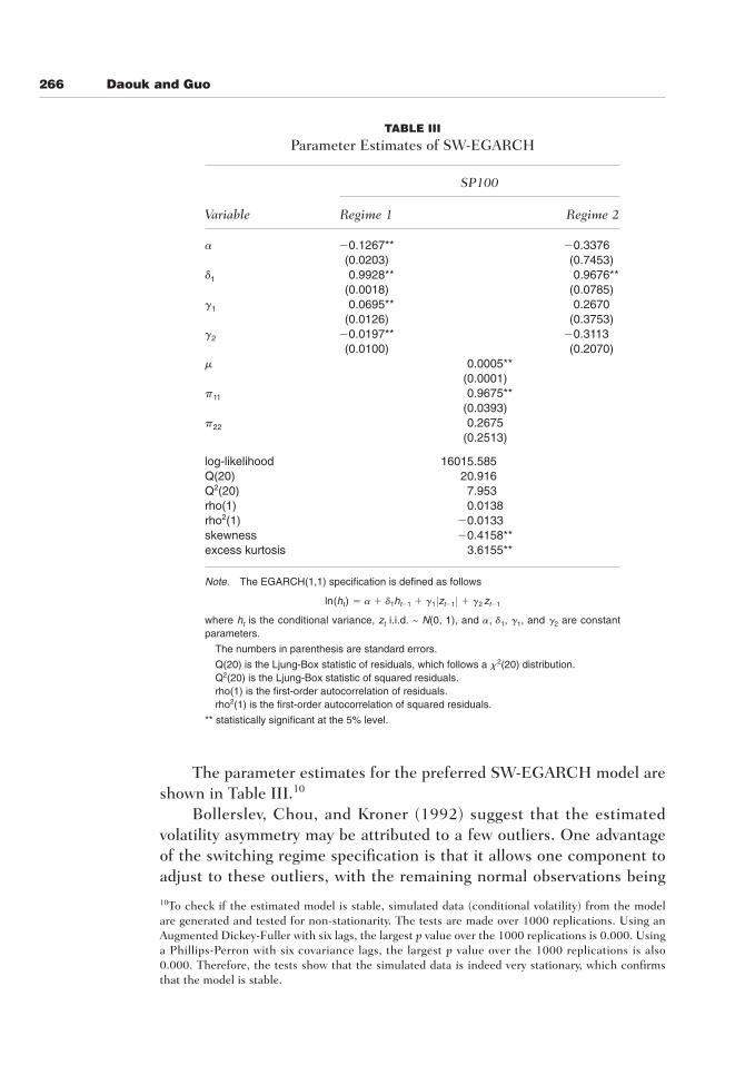
The parameter estimates for the preferred SW-EGARCH model areshown in Table III.10

Bollerslev, Chou, and Kroner (1992) suggest that the estimatedvolatility asymmetry may be attributed to a few outliers. One advantageof the switching regime specification is that it allows one component toadjust to these outliers, with the remaining normal observations being


estimated by another component. In this case, the influence of the out-liers is isolated. Table III shows that g2 is significantly negative in thetranquil regime. The coefficient g2 is large in the volatile regime, albeitnot statistically significant because of the large standard error. Thisseems to indicate that volatility asymmetry is present in both the tranquiland volatile regimes. d1 is larger in the tranquil regime than in thevolatile regime, which seems to indicate that the tranquil regime exhibitsmore persistence than the volatile regime. This is consistent with litera-ture that shows that removing exceptionally volatile observations (the1987 crash for example) increases the persistence parameters of ARCHmodels (see for example Blair et al., 1998).

The standardized residual diagnostics are reported at thebottom of Table III. If the model is correctly specified, the null hypothe-sis of zero autocorrelation of standardized residuals and squared stan-dardized residuals should not be rejected. We indeed find that Q(20) andQ2(20) are not significantly different from zero. The results demonstratethat there is no evidence of autocorrelation in the squared residuals,which suggests that the SW-EGARCH model provides an adequatedescription of the data.

The Jarque-Bera normality tests still reject the null of normality ofstandardized residuals. However, comparing with the raw residuals inTable I, we can see that there is a dramatic reduction in the skewnessand kurtosis.

The mean of the conditional variance of the first regime is found tobe 0.000083. That of the second regime is 0.000568. This clearly showsthat the second regime is much more volatile than the first regime. Theratio of the variances is about 6.8. The unconditional probability of beingin the tranquil regime is 0.783, which indicates that during the period ofinterest (4861 days), roughly 1053 days were in the volatile regime.

MONTE CARLO INTEGRATION OF OPTION PRICES

At this juncture, it has been shown that the SW-EGARCH specificationfor volatility is a better fit to security returns than a simple GARCH. Inthis section, values for options on volatility are computed using differentspecifications for the volatility process. The objective is to assess theeconomic significance of the impact of the volatility index properties onthe value of the options. More specifically, we want to quantify thedifference in the options value between the different volatility specifica-tions analyzed in the previous section.

(et�2ht)

268 Daouk and Guo

The focus is on the switching and asymmetry properties of volatility.However, the issue of risk premium has to be addressed. As statedbefore, volatility is not a traded asset. Therefore, a volatility option pric-ing model needs to account for that by making assumptions about theexpected premium for volatility risk. G-L assume that it is proportional tothe level of volatility. This paper focuses on the assumption for theunderlying process of volatility. Therefore, we want to show that regard-less of the choice of risk premium, the process in G-L leads to a severemispricing in the options. To attain this objective, option values that arediscounted by the risk-free rate alone are computed. This is done forsimplicity. This is appropriate because we are not proposing a new pric-ing model, but rather highlighting the impact of assumptions about theunderlying asset on the price of the options. All what is needed is to com-pare values computed using different underlying processes irrespectiveof the discount factor. In fact, if those values are discounted using thesame discount factor, the relative difference between the values based ondifferent underlying processes will remain the same. In the next section,the results are replicated using a discount factor that incorporates a riskpremium. It is shown that in this case, the conclusions remain the same.

The procedure to compute option prices is as follows:

1. The parameters from the volatility models estimated previously areused to generate a simulated volatility index.11

2. The payoff at maturity of a European call option on the volatilityprocess is computed.

3. The payoff is discounted using the appropriate discount rate.4. The procedure is repeated for 100,000 independent replications.5. The value of the option is then computed as the average of all option

discounted payoffs at maturity over the 100,000 replications.12

11We use a technique known as synchronization (see Law and Kelton, 1991). This implies twothings. First, we adopt the same seed for the random number generator for each model. Second, wemake sure to adopt the same sequence of generation of random variates for each model. This isimportant since we need to generate more random variates for the switching models to allow the ran-dom choice of different regimes. For that reason, for the uni-regime models, we generate the samesequence of random variates as for the switching models, but we simply discard those that are meantto determine the regime. The result from synchronization is that the random variates used by eachmodel are identical. This ensures that the differences in option values will arise uniquely from thedifference in assumed volatility processes (as opposed to the random variates generated).12Standard errors are also computed for each option value. Given that a large number of replications(100,000) are made, the standard errors are extremely small compared to the difference betweenvalues computed from different processes. For that reason, statistical significance holds for all ourresults. As an indication, the largest standard error of any option value in our study is 0.0457. As willbe seen, this is dwarfed by the difference between option values computed with different volatilityprocesses. For that reason, the issue of statistical significance will be omitted throughout the expo-sition of the results.


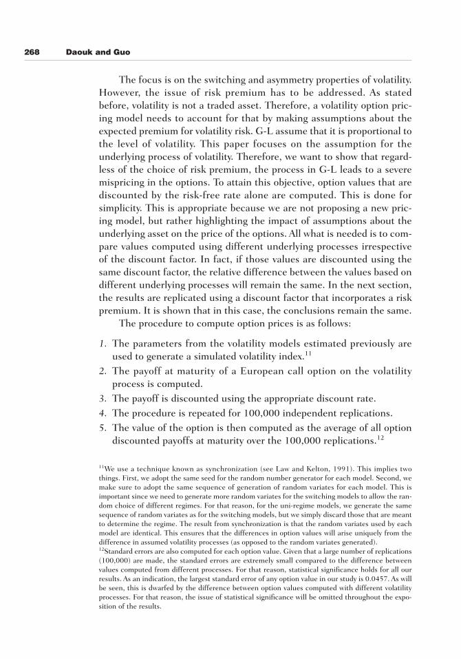
Call option values are computed for different time to maturity(1 month to 12 months), different exercise prices (5 to 30), and differentvolatility index (underlying asset) values (5 to 40). Figures 1, 3, and 5present three-dimensional graphs depicting option values from the SW-EGARCH for different sets of characteristics. Figures 2, 4, and 6 providethree-dimensional graphs presenting the difference in option valuesbetween those based on the SW-EGARCH and those based on theGARCH process. This will allow us to assess if the difference in optionvalues between the two processes is large enough as compared to theoption values under SW-EGARCH. This will tell us if the assumptions inG-L are acceptable approximations or not.

Figure 1 gives option values for different exercise prices and time tomaturity.

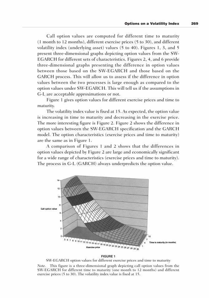
The volatility index value is fixed at 15. As expected, the option valueis increasing in time to maturity and decreasing in the exercise price.The more interesting figure is Figure 2. Figure 2 shows the difference inoption values between the SW-EGARCH specification and the GARCHmodel. The option characteristics (exercise prices and time to maturity)are the same as in Figure 1.

A comparison of Figures 1 and 2 shows that the differences inoption values depicted by Figure 2 are large and economically significantfor a wide range of characteristics (exercise prices and time to maturity).The process in G-L (GARCH) always underpredicts the option value.

FIGURE 1SW-EGARCH option values for different exercise prices and time to maturity

Note. This figure is a three-dimensional graph depicting call option values from theSW-EGARCH for different time to maturity (one month to 12 months) and differentexercise prices (5 to 30). The volatility index value is fixed at 15.

270 Daouk and Guo

FIGURE 2Difference between SW-EGARCH and GARCH-based option values

for different exercise prices and time to maturityNote. This figure is a three-dimensional graph presenting the difference in call optionvalues between those based on the SW-EGARCH and those based on the GARCHprocesses for different time to maturity (one month to 12 months) and different exerciseprices (5 to 30). The volatility index value is fixed at 15.

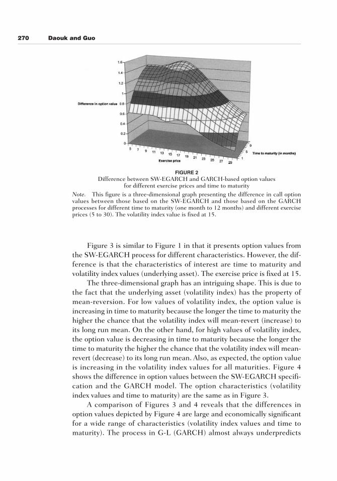
Figure 3 is similar to Figure 1 in that it presents option values fromthe SW-EGARCH process for different characteristics. However, the dif-ference is that the characteristics of interest are time to maturity andvolatility index values (underlying asset). The exercise price is fixed at 15.

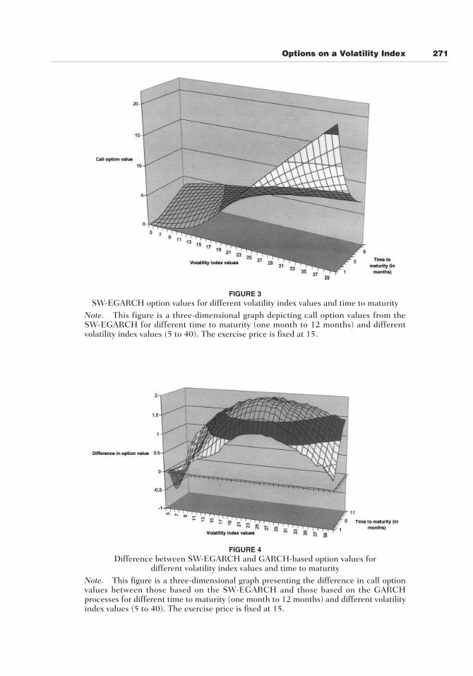
The three-dimensional graph has an intriguing shape. This is due tothe fact that the underlying asset (volatility index) has the property ofmean-reversion. For low values of volatility index, the option value isincreasing in time to maturity because the longer the time to maturity thehigher the chance that the volatility index will mean-revert (increase) toits long run mean. On the other hand, for high values of volatility index,the option value is decreasing in time to maturity because the longer thetime to maturity the higher the chance that the volatility index will mean-revert (decrease) to its long run mean. Also, as expected, the option valueis increasing in the volatility index values for all maturities. Figure 4shows the difference in option values between the SW-EGARCH specifi-cation and the GARCH model. The option characteristics (volatilityindex values and time to maturity) are the same as in Figure 3.

A comparison of Figures 3 and 4 reveals that the differences inoption values depicted by Figure 4 are large and economically significantfor a wide range of characteristics (volatility index values and time tomaturity). The process in G-L (GARCH) almost always underpredicts


FIGURE 3SW-EGARCH option values for different volatility index values and time to maturity

Note. This figure is a three-dimensional graph depicting call option values from theSW-EGARCH for different time to maturity (one month to 12 months) and differentvolatility index values (5 to 40). The exercise price is fixed at 15.

FIGURE 4Difference between SW-EGARCH and GARCH-based option values for

different volatility index values and time to maturityNote. This figure is a three-dimensional graph presenting the difference in call optionvalues between those based on the SW-EGARCH and those based on the GARCHprocesses for different time to maturity (one month to 12 months) and different volatilityindex values (5 to 40). The exercise price is fixed at 15.

272 Daouk and Guo

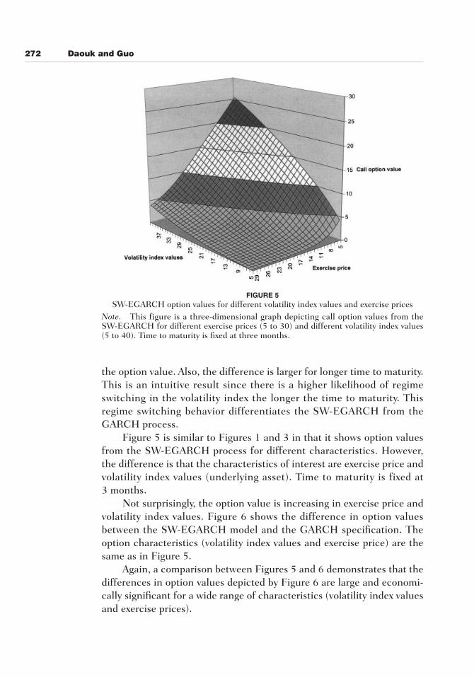
FIGURE 5SW-EGARCH option values for different volatility index values and exercise prices

Note. This figure is a three-dimensional graph depicting call option values from theSW-EGARCH for different exercise prices (5 to 30) and different volatility index values(5 to 40). Time to maturity is fixed at three months.

the option value. Also, the difference is larger for longer time to maturity.This is an intuitive result since there is a higher likelihood of regimeswitching in the volatility index the longer the time to maturity. Thisregime switching behavior differentiates the SW-EGARCH from theGARCH process.

Figure 5 is similar to Figures 1 and 3 in that it shows option valuesfrom the SW-EGARCH process for different characteristics. However,the difference is that the characteristics of interest are exercise price andvolatility index values (underlying asset). Time to maturity is fixed at3 months.

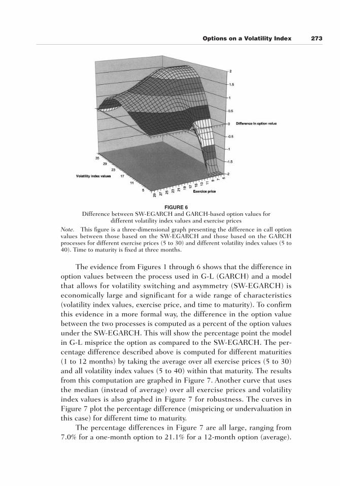
Not surprisingly, the option value is increasing in exercise price andvolatility index values. Figure 6 shows the difference in option valuesbetween the SW-EGARCH model and the GARCH specification. Theoption characteristics (volatility index values and exercise price) are thesame as in Figure 5.

Again, a comparison between Figures 5 and 6 demonstrates that thedifferences in option values depicted by Figure 6 are large and economi-cally significant for a wide range of characteristics (volatility index valuesand exercise prices).


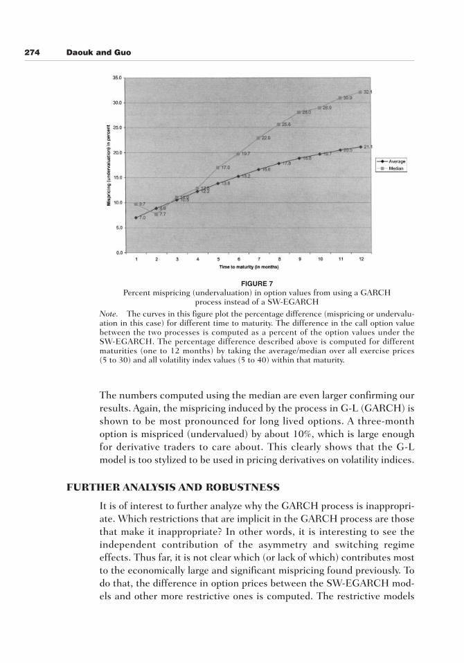
The evidence from Figures 1 through 6 shows that the difference inoption values between the process used in G-L (GARCH) and a modelthat allows for volatility switching and asymmetry (SW-EGARCH) iseconomically large and significant for a wide range of characteristics(volatility index values, exercise price, and time to maturity). To confirmthis evidence in a more formal way, the difference in the option valuebetween the two processes is computed as a percent of the option valuesunder the SW-EGARCH. This will show the percentage point the modelin G-L misprice the option as compared to the SW-EGARCH. The per-centage difference described above is computed for different maturities(1 to 12 months) by taking the average over all exercise prices (5 to 30)and all volatility index values (5 to 40) within that maturity. The resultsfrom this computation are graphed in Figure 7. Another curve that usesthe median (instead of average) over all exercise prices and volatilityindex values is also graphed in Figure 7 for robustness. The curves inFigure 7 plot the percentage difference (mispricing or undervaluation inthis case) for different time to maturity.

The percentage differences in Figure 7 are all large, ranging from7.0% for a one-month option to 21.1% for a 12-month option (average).

FIGURE 6Difference between SW-EGARCH and GARCH-based option values for

different volatility index values and exercise pricesNote. This figure is a three-dimensional graph presenting the difference in call optionvalues between those based on the SW-EGARCH and those based on the GARCHprocesses for different exercise prices (5 to 30) and different volatility index values (5 to40). Time to maturity is fixed at three months.

274 Daouk and Guo

FIGURE 7Percent mispricing (undervaluation) in option values from using a GARCH

process instead of a SW-EGARCHNote. The curves in this figure plot the percentage difference (mispricing or undervalu-ation in this case) for different time to maturity. The difference in the call option valuebetween the two processes is computed as a percent of the option values under theSW-EGARCH. The percentage difference described above is computed for differentmaturities (one to 12 months) by taking the average/median over all exercise prices (5 to 30) and all volatility index values (5 to 40) within that maturity.

The numbers computed using the median are even larger confirming ourresults. Again, the mispricing induced by the process in G-L (GARCH) isshown to be most pronounced for long lived options. A three-monthoption is mispriced (undervalued) by about 10%, which is large enoughfor derivative traders to care about. This clearly shows that the G-Lmodel is too stylized to be used in pricing derivatives on volatility indices.

FURTHER ANALYSIS AND ROBUSTNESS

It is of interest to further analyze why the GARCH process is inappropri-ate. Which restrictions that are implicit in the GARCH process are thosethat make it inappropriate? In other words, it is interesting to see theindependent contribution of the asymmetry and switching regimeeffects. Thus far, it is not clear which (or lack of which) contributes mostto the economically large and significant mispricing found previously. Todo that, the difference in option prices between the SW-EGARCH mod-els and other more restrictive ones is computed. The restrictive models


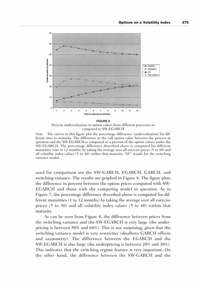
used for comparison are the SW-GARCH, EGARCH, GARCH, andswitching variance. The results are graphed in Figure 8. The figure plotsthe difference in percent between the option prices computed with SW-EGARCH and those with the competing model in question. As inFigure 7, the percentage difference described above is computed for dif-ferent maturities (1 to 12 months) by taking the average over all exerciseprices (5 to 30) and all volatility index values (5 to 40) within thatmaturity.

As can be seen from Figure 8, the difference between prices fromthe switching variance and the SW-EGARCH is very large (the under-pricing is between 50% and 60%). This is not surprising, given that theswitching variance model is very restrictive (disallows GARCH effectsand asymmetry). The difference between the EGARCH and theSW-EGARCH is also large (the underpricing is between 20% and 30%).This indicates that the switching regime feature is very important. Onthe other hand, the difference between the SW-GARCH and the

FIGURE 8Percent undervaluation in option values from different processes as

compared to SW-EGARCHNote. The curves in this figure plot the percentage difference (undervaluation) for dif-ferent time to maturity. The difference in the call option value between the process inquestion and the SW-EGARCH is computed as a percent of the option values under theSW-EGARCH. The percentage difference described above is computed for differentmaturities (one to 12 months) by taking the average over all exercise prices (5 to 30) andall volatility index values (5 to 40) within that maturity. “SV” stands for the switchingvariance model.

276 Daouk and Guo

SW-EGARCH is rather small (between 2% and 6%). This shows that thevolatility asymmetry feature is much less important than the regimeswitching in terms of option pricing. Finally, the underpricing from theGARCH process (as compared to the SW-EGARCH) is less than that ofthe EGARCH. This indicates that accounting for asymmetry withoutregime switching can make things worse (especially for short maturities).

Next, the consequences on our previous results of relaxing theassumption that volatility risk is not priced, is examined. G-L followWiggins (1987), Stein and Stein (1991), and others in assuming that theexpected premium for volatility risk is proportional to the level ofvolatility, zV where z is a constant parameter. This assumption is similarto the implications of general equilibrium models such as Cox, Ingersoll,and Ross (1985), Hemler and Longstaff (1991), and Longstaff andSchwartz (1992), in which risk premia in security returns are propor-tional to the level of volatility. We replicate the results in Figure 7 for thecase where volatility risk is priced. The only difference in option pricescomputed in this section from those presented before is in the discountfactor. Previously, the discount factor was assumed to be the risk-freerate. In this section however, the discount factor is defined to be the risk-free rate plus a risk premium. The risk premium is a linear function ofthe level of volatility (zV). z is chosen to be equal to 0.25. The choice ofthis coefficient is somewhat arbitrary. However, it seemed to deliver real-istic risk premia for different levels of volatility. Moreover, we checkedthe robustness of our results by trying a wide range of values for z. Theresults were extremely close. Figure 9 replicates the results fromFigure 7 with the addition of the risk premium described above.

A comparison between the two figures reveals that they are very sim-ilar. Essentially, the mispricing between the GARCH and the SW-EGARCH processes are as described before. There is a very smalldecrease in the mispricing when the risk premium is taken into account(less than 1% in all cases). Therefore, assuming a risk premium asopposed to just using the risk-free rate does not alter our results.

Finally, we analyze volatility index data (VIX). We want to make surethat the SW-EGARCH is also a better fit than GARCH in the case ofVIX. Since the options are written on the volatility index itself, we needto prove that VIX is more consistent with SW-EGARCH than it is withGARCH. We obtain VIX daily data from the Chicago Board OptionsExchange. Our data is from the period January 2, 1986 to December 6,2002. We estimate two models. The first one is the analog to a GARCHprocess:

(16)VIXt � a � d1VIXt�1 � et


FIGURE 9Percent undervaluation in option values from using a GARCH process instead

of a SW-EGARCH (accounting for volatility risk premium)Note. The curves in this figure plot the percentage difference (undervaluation) for dif-ferent time to maturity. The difference in the call option value between the two processesis computed as a percent of the option values under the SW-EGARCH. The percentagedifference described above is computed for different maturities (one to 12 months) bytaking the average/median over all exercise prices (5 to 30) and all volatility index values(5 to 40) within that maturity. The discount factor is defined to be the risk-free rate plusa risk premium factor. The risk premium factor is a linear function of the level ofvolatility (zV). z is chosen to be equal to 0.25

The second model we estimate is the analog to a SW-EGARCH:

(17)

where VIXt is the volatility index, and is the residual from This residual term introduces asymmetry in the model analo-

gously to SW-EGARCH, by allowing the sign (and magnitude) of thereturn on the S&P 100 to affect the volatility index. Also, note that thesecond model is a regime-switching model.

The models are estimated using a normal likelihood for the errorterms. The d1 coefficient in the model analog to GARCH is estimated tobe 0.95. As expected, this indicates that the volatility index is highly per-sistent. The coefficient estimates for the second model are qualitativelysimilar to the SW-EGARCH model, and are available upon request fromthe authors. The key here is to figure out which model fits the data best.Since the two models are not nested, we use the penalized Akaiki

m � ret�1.Rt �ret�1

ln(VIXt) � a � d1VIXt�1 � g1 ` ret�1

1VIXt�1

` � g2

ret�1

1VIXt�1

� et

278 Daouk and Guo

Information Criterion and the Baysian Information Criterion. The AIC is20079 for the GARCH analog and 13395 for the SW-EGARCH analog,respectively. As can be seen, the AIC for the SW-EGARCH analog ismuch smaller than that of the GARCH analog. This indicates that theSW-EGARCH representation is a much better fit to the VIX data than theGARCH representation. The BIC is 20098 for the GARCH analog and13471 for the SW-EGARCH analog, respectively. This confirms the AICresults. To conclude, we are now comfortable that our results related tothe conditional volatility carry through to the observed volatility index.

CONCLUSION

In this paper, it is shown that volatility index option pricing models thatdo not take into account the regime switching and asymmetry propertiesof volatility, undervalue a three-month option by about 10%. Such amodel was proposed in Grunbichler and Longstaff (1996). Their modelis based on modeling volatility as a GARCH process. For that reason,their model does not take into account the asymmetric relation betweenvolatility and returns. More importantly, their model does not accountfor the fact that volatility might be subject to different regimes.Switching Regime Asymmetric GARCH is used to model the generatingprocess of security returns. The model specifies the conditional varianceof security returns as following two regimes possessing different charac-teristics (tranquil regime and volatile regime). The comparison betweenthe switching regime models and the traditional uni-regime modelsamong GARCH, EGARCH, and GJR-GARCH demonstrates that theSW-EGARCH model fits the data best. Next, the values of European calloptions written on a volatility index are computed using Monte Carlointegration. Option values based on the SW-EGARCH model are com-pared with those based on the traditional GARCH specification. It isfound that the option values obtained from the different processes arevery different. This clearly shows that the G-L model is too stylized to beused in pricing derivatives on volatility indices. Therefore, uni-regimemodels for volatility should be used with caution because they are basedon the assumption of parametric homogeneity and do not allow regimeswitching. There is an urgent need for research to develop volatilityderivatives pricing models that account for volatility asymmetry andvolatility regime switching. This will need to be done before derivativeson volatility indices are introduced by the major futures and optionsexchanges of the world. Finally, we propose three promising avenues forfuture research. An alternative approach to address the persistence in


volatility (or spurious persistence) issue is that of Bollerslev andMikkelsen (1996) and Baillie, Bollerslev, and Mikkelsen (1996). Theypropose and use a fractionally integrated GARCH, which implies a slowhyperbolic rate of decay for the influence of lagged squared innovations.It might be worthwhile to explore volatility option pricing using theFIGARCH model. This study has focused on call options. It might be aworthwhile extension to check that the results still hold with put options.

BIBLIOGRAPHY

Akgiray, V. (1989). Conditional heteroskedasticity in time series of stockreturns: Evidence and forecasts. Journal of Business, 62, 55–80.

Ang, A., & Bekaert, G. (1998). Regime switches in interest rates. Working paper,Columbia University.

Baillie, R. T., Bollerslev, T., & Mikkelsen, H. O. (1996). Fractionally integratedgeneralized autoregressive conditional heteroskedasticity. Journal ofEconometrics, 74, 3–30.

Bera, A. K., & Higgins, M. L. (1993). ARCH models: Properties, estimation andtesting. Journal of Economic Surveys, 7, 305–366.

Billio, M., & Pelizzon, L. (1996). Pricing option with switching regime volatility.Working paper, University of Venice.

Black, F. (1976). Studies of stock price volatility changes. Proceedings of theBusiness and Economic Statistics Section, American Statistical Association,177–181.

Black, F., & Scholes, M. (1973). The pricing of options and corporate liabilities.Journal of Political Economy, 81, 637–654.

Blair, B., Poon, S., & Taylor, S. (1998). Asymmetric and crash effects in stockvolatility for the S&P 100 Index and its constituents. Working paper,Lancaster University.

Böhning, D., Dietz, E., Schaub, R., Schlattmann, P., & Lindsay, B. G. (1994).The distribution of the likelihood ratio for mixtures of densities from theone-parameter exponential family. Annals of the Institute of StatisticalMathematics, 46, 373–388.

Bollen, N. (1998). Valuing options in regime-switching models. Journal ofDerivatives, 6, 38–49.

Bollen, N., Gray, S., & Whaley, R. (2000). Regime-switching in foreignexchange rates: Evidence from currency options. Journal of Econometrics,94, 239–276.

Bollerslev, T. (1986). Generalized autoregressive conditional heteroskedasticity.Journal of Econometrics, 31, 307–327.

Bollerslev, T., Chou, R. Y., & Kroner, K. F. (1992). ARCH modeling in finance.Journal of Econometrics, 52, 5–59.

Bollerslev, T., & Engle, R. F. (1986). Modelling the persistence of conditionalvariances. Econometric Reviews, 5, 1–50.

Bollerslev, T., & Mikkelsen, H. O. (1996). Modeling and pricing long memory instock market volatility. Journal of Econometrics, 73, 151–184.

280 Daouk and Guo

Brenner, M., & Galai, D. (1989). New financial instruments for hedgingchanges in volatility. Financial Analysts Journal, July/August, 61–65.

Cai, J. (1994). A Markov model of switching-regime ARCH. Journal of Businessand Economic Statistics, 12, 309–316.

Campbell, S., & Li, C. (1999). Option pricing with unobserved and regime-switching volatility. Working paper, University of Pennsylvania.

Cox, J., Ingersoll, J., & Ross, S. (1985). A theory of the term structure of inter-est rates. Econometrica, 53, 385–408.

Dahlquist, M., & Gray, S. (2000). Regime-switching and interest rates in theEuropean Monetary System. Journal of International Economics, forth-coming.

Duan, J. (1995). The GARCH option pricing model. Mathematical Finance, 5,13–32.

Duan, J., Popova, I., & Ritchken, P. (1999). Option pricing under regimeswitching. Working paper, Hong Kong University of Science andTechnology.

Engle, R. (1982). Autoregressive conditional heteroskedasticity with estimatesof the variance of U.K. inflation. Econometrica, 50, 987–1008.

Fleming, J., Ostdiek, B., & Whaley, R. (1995). Predicting stock market volatility:A new measure. Journal of Futures Markets, 15, 265–302.

Fornari, F., & Mele, A. (1997). Sign- and volatility-switching ARCH models:Theory and application to international stock markets. Journal of AppliedEconometrics, 12, 49–67.

French, K., Schwert, W., & Stambaugh, R. (1987). Expected stock returns andvolatility. Journal of Financial Economics, 19, 3–29.

Glosten, L., Jagannathan, R., & Runkle, D. (1993). On the relation between theexpected value and the volatility of the nominal excess return on stocks.Journal of Finance, 68, 1779–1801.

Gray, S. (1996a). Modeling the conditional distribution of interest rates as aregime switching process. Journal of Financial Economics, 42, 27–62.

Gray, S. (1996b). Regime-switching in Australian interest rates. Accounting andFinance, 36, 65–88.

Grunbichler, A., & Longstaff, F. (1996). Valuing futures and options onvolatility. Journal of Banking and Finance, 20, 985–1001.

Hamilton, J. (1988). Rational-expectations econometric analysis of changes inregime: An investigation of the term structure of interest rates. Journal ofEconomic Dynamics and Control, 12, 385–423.

Hamilton, J. (1989). A new approach to the economic analysis of nonstationarytime series and the business cycle. Econometrica, 57, 357–384.

Hamilton, J. (1994). Time series analysis. Princeton, NJ: Princeton UniversityPress.

Hamilton, J., & Susmel, R. (1994). Autoregressive conditional heteroskedasticityand changes in regime. Journal of Econometrics, 64, 307–333.

Hemler, M., & Longstaff, F. (1991). General equilibrium stock index futuresprices: Theory and empirical evidence. Journal of Financial andQuantitative Analysis, 26, 287–308.


Heston, S. (1993). A closed form solution for options with stochastic volatilitywith applications to bond and currency options. Review of FinancialStudies, 6, 327–343.

Heston, S., & Nandi, S. (1999). A closed-form GARCH option pricing model.Review of Financial Studies, forthcoming.

Hull, J., & White, A. (1987). Pricing options with stochastic volatilities. Journalof Finance, 42, 281–300.

Kim, D., & Kon, S. J. (1999). Structural change and time dependence in modelsof stock returns. Journal of Empirical Finance, 6, 283–308.

Kon, S. J. (1984). Models of stocks returns—A comparison. Journal of Finance,39, 147–165.

Law, A. M., & Kelton, W. D. (1991). Simulation modeling & analysis (2nd ed.).New York: McGraw-Hill.

Longstaff, F., & Schwartz, E. (1992). Interest rate volatility and the term struc-ture: A two-factor general equilibrium model. Journal of Finance, 47,1259–1282.

Mandelbrot, B. (1963). The variation of certain speculative prices. Journal ofBusiness, 36, 394–419.

Nelson, D. (1990). ARCH models as diffusion approximations. Journal ofEconometrics, 45, 7–38.

Nelson, D. (1991). Conditional heteroskedasticity in asset returns: A newapproach. Econometrica, 59(2), 347–370.

Norden, S. (1995). Regime switching as a test for exchange rate bubbles.Working paper, Bank of Canada.

Norden, S., & Schaller, H. (1993). Regime switching in stock market returns.Manuscript, Bank of Canada and Carleton University.

Perron, P. (1989). The great crash, the oil price shock, and the unit root hypoth-esis. Econometrica, 57, 1361–1401.

Ritchey, R. (1990). Call option valuation for discrete normal mixtures. Journalof Financial Research, 13, 285–296.

Rockinger, M. (1994). Regime switching: Evidence for the French stock market.Mimeo, HEC.

Schobel, R., & Zhu, J. (1998). Stochastic volatility with an Ornstein-UhlenbeckProcess: An extension. Working paper, University of Tuebingen.

Stein, E., & Stein, C. (1991). Stock price distributions with stochastic volatility:An analytic approach. Review of Financial Studies, 4, 727–752.

Susmel, R. (1994). Switching volatility in international equity markets. Workingpaper, University of Houston.

Susmel, R. (1998a). Switching volatility in Latin American emerging markets.Emerging Markets Quarterly, 2.

Susmel, R. (1998b). A switching volatility model for inflation: International evi-dence. Working paper, University of Houston.

Taylor, S., & Xu, X. (1994). Implied volatility shapes when price and volatilityshocks are correlated. Working paper, Lancaster University.

Vosti, C. (1993). CBOE creates new index to deal with market volatility.Pensions & Investments, February 8, 1993.

282 Daouk and Guo

Walsh, D. (1999). Some exotic options under symmetric and asymmetric condi-tional volatility of returns. Journal of Multinational Financial Management,9, 403–417.

Weiss, A. (1986). Asymptotic theory for ARCH models: Estimation and testing.Econometric Theory, 2, 107–131.

Whaley, R. (1993). Derivatives on market volatility: Hedging tools long overdue.Journal of Derivatives, Fall, 71–84.

Whaley, R. (2000). The investor fear gauge. Working paper, Duke University.Wiggins, J. (1987). Option values under stochastic volatility: Theory and empir-

ical estimates. Journal of Financial Economics, 19, 351–372.

switching asymmetric garch and options on a volatility index

Documents