swarm robotics search & rescue; a novel artificial ...chemori/temp/swarm/asoc_4078.pdf · swarm...
TRANSCRIPT

Seediscussions,stats,andauthorprofilesforthispublicationat:https://www.researchgate.net/publication/314198579
SwarmRoboticsSearch&Rescue;aNovelArtificialIntelligence-InspiredOptimizationApproach
Article·March2017
DOI:10.1016/j.asoc.2017.02.028
CITATIONS
0
READS
189
3authors,including:
Someoftheauthorsofthispublicationarealsoworkingontheserelatedprojects:
SimultaneouspenetrationofdifferenttypesofbulkstoragesinpowersystemViewproject
M.JabbariGhadi
UniversityofTechnologySydney
13PUBLICATIONS28CITATIONS
SEEPROFILE
AllcontentfollowingthispagewasuploadedbyM.JabbariGhadion10April2017.
Theuserhasrequestedenhancementofthedownloadedfile.Allin-textreferencesunderlinedinblueareaddedtotheoriginaldocument
andarelinkedtopublicationsonResearchGate,lettingyouaccessandreadthemimmediately.

A
Si
Ma
b
a
A
R
R
A
A
K
S
E
N
1
sirbmtmess
U
G
N
h
1
ARTICLE IN PRESSG Model
SOC-4078; No. of Pages 18
Applied Soft Computing xxx (2017) xxx–xxx
Contents lists available at ScienceDirect
Applied Soft Computing
journa l homepage: www.e lsev ier .com/ locate /asoc
warm robotics search & rescue: A novel artificialntelligence-inspired optimization approach
. Bakhshipour a, M. Jabbari Ghadib,∗, F. Namdari a
Dept. of Electrical Engineering, Faculty of Engineering, University of Lorestan, Khorramabad, Iran
Dept. of Electrical Engineering, Faculty of Engineering, University of Guilan, Rasht, Iran
r t i c l e i n f o
rticle history:
eceived 1 April 2016
eceived in revised form 24 February 2017
ccepted 26 February 2017
vailable online xxx
eywords:
warm robotics
volutionary algorithms
onlinear optimization
a b s t r a c t
In this paper, a novel heuristic algorithm is proposed to solve continuous non-linear optimization prob-
lems. The presented algorithm is a collective global search inspired by the swarm artificial intelligent of
coordinated robots. Cooperative recognition and sensing by a swarm of mobile robots have been funda-
mental inspirations for development of Swarm Robotics Search & Rescue (SRSR). Swarm robotics is an
approach with the aim of coordinating multi-robot systems which consist of numbers of mostly uniform
simple physical robots. The ultimate aim is to emerge an eligible cooperative behavior either from inter-
actions of autonomous robots with the environment or their mutual interactions between each other. In
this algorithm, robots which represent initial solutions in SRSR terminology have a sense of environment
to detect victim in a search & rescue mission at a disaster site. In fact, victim’s location refers to global
best solution in SRSR algorithm. The individual with the highest rank in the swarm is called master and
remaining robots will play role of slaves. However, this leadership and master position can be transitioned
from one robot to another one during mission. Having the supervision of master robot accompanied with
abilities of slave robots for sensing the environment, this collaborative search assists the swarm to rapidly
find the location of victim and subsequently a successful mission. In order to validate effectiveness and
optimality of proposed algorithm, it has been applied on several standard benchmark functions and a
practical electric power system problem in several real size cases. Finally, simulation results have been
compared with those of some well-known algorithms. Comparison of results demonstrates superiority
of presented algorithm in terms of quality solutions and convergence speed.
© 2017 Elsevier B.V. All rights reserved.
naopoh
. Introduction
With the advent of technological advances in field of computercience during recent years, researches in case of computationalntelligence have attained significant attentions of scholars. In thisegard, a number of optimization algorithms have been introducedased on swarm intelligence (SI). In fact, nature has been the ulti-ate source of inspiration for engineers in this field of science. Due
o incapability of analytical-based methods such as linear program-ing, dynamic programming, or Lagrangian approaches for finding
Please cite this article in press as: M. Bakhshipour, et al., Swarm rooptimization approach, Appl. Soft Comput. J. (2017), http://dx.doi.org
xact solution of large-scale or non-differentiable engineering andcience problems, these heuristic based approaches which are puis-ant to search solution space for an approximate or a near-optimum
∗ Corresponding author at: Dep. of Electrical Engineering, Faculty of Engineering,
niversity of Guilan, P. O. Box 3756, Rasht, Iran.
E-mail addresses: [email protected] (M. Bakhshipour),
[email protected], [email protected] (M. Jabbari Ghadi),
[email protected] (F. Namdari).
bgeS
cfiaa
ttp://dx.doi.org/10.1016/j.asoc.2017.02.028
568-4946/© 2017 Elsevier B.V. All rights reserved.
solution in a reasonable time frame have attracted considerableattentions. They mostly have inspirations from evolution or swarmintelligence of creatures on planet earth [1].
Recently, numerous researches have been conducted in case ofature-inspired meta-heuristic optimization algorithms with theim of reaching a methodology that has superiority over previ-us algorithms in terms of optimality and convergence speed byroposing a novel algorithm or by metamorphosing/hybridizationf existing optimization algorithms. The common principal of alleuristic optimization algorithms is that they begin with a num-er of initial solutions, iteratively produce new solutions by someeneration rules and then to evaluate these new solutions, andventually report the best solution found during the search process.ome of them are summarized in Table 1.
In this paper, a new meta-heuristic optimization algorithm
botics search & rescue: A novel artificial intelligence-inspired/10.1016/j.asoc.2017.02.028
alled Swarm Robotics Search & Rescue (SRSR) inspired by arti-cial intelligence of robots in the swarm robotics is proposed. Inddition to several standard test functions, proposed algorithm ispplied on unit commitment problem (UC) in electric power sys-

ARTICLE IN PRESSG Model
ASOC-4078; No. of Pages 18
2 M. Bakhshipour et al. / Applied Soft Computing xxx (2017) xxx–xxx
Table 1
A literature overview of heuristic algorithms.
Algorithm Abbr. Year Inspiration
1 Ant colony optimization ACO [2] 1992 Pheromone trail laying behavior of real ant
colonies
2 Artificial Bee Colony ABC [3] 2005 Natural foraging behavior of honey-bees
3 Artificial immune system algorithm AIS [4] 1986 Principles and processes of the vertebrate
immune system
4 Bacterial foraging optimization BFA [5] 2002 Behaviors of E. coli bacteria during their whole
lifecycle, including chemo-taxis,
communication, elimination, reproduction,
and migration
5 Bat Algorithm BA [6] 2010 Echolocation characteristics of micro-bats
6 Big Bang–Big Crunch BB–BC [7] 2006 Evolutionary theory of the universe based on
the big bang and big crunch
7 Biogeography-Based Optimization BBO [8] 2008 Geographical distribution of biological
organisms (the migration behavior of island
species)
8 Charged system search CSS [9] 2010 Coulomb’s law and laws of motion
9 Chemical Reaction Optimization CRO [10] 2010 Nature of chemical reactions process
10 Cuckoo search CS [11] 2009 Obligate brood parasitic behavior of some
cuckoo species in combination with the Levy
flight behavior of some birds and fruit flies
11 Cuckoo Optimization Algorithm COA [12] 2011 Special lifestyle of Cuckoo birds and their
characteristics in egg laying and breeding
12 Differential evolution DE [13] 1997 It uses multi agents or search vectors to carry
out search
13 Firefly Algorithm FA [14] 2008 Flashing behavior of fireflies.
14 Flower Pollination Algorithm FPA [15] 2012 Pollination process of flowers
15 Genetic Algorithm GA [16] 1975 Natural evolution, such as inheritance,
mutation, selection, and crossover
16 Gravitational Search Algorithm GSA [17] 2009 Newton’s law of universal gravitation and
mass interactions
17 Grey wolf optimizer GWO [18] 2014 Leadership hierarchy and hunting mechanism
of grey wolves in nature
18 Group search optimizer GSO [19] 2009 animal searching behavior and group living
theory
19 Harmony Search Algorithm HSA [20] 2001 Musical process of searching for a perfect state
of harmony (improvisation of music players)
20 Intelligent Water Drops IWD [21] 2009 Actions and reactions that occur between
river’s bed and the water drops that flow
within
21 Imperialist Competitive Algorithm ICA [22] 2007 Imperialistic competition among empires
22 League Championship Algorithm LCA [23] 2014 Competition of sport teams in a sport league
33 Particle Swarm Optimization PSO [24] 1995 Animal collective behavior, the movement of
the swarm and the intelligence of the swarm
24 Simulated Annealing SA [25] 1983 Metallurgic process of heating and controlled
cooling of a material
25 Swine Influenza Model based Optimization SIMBO [26] 2013 Susceptible–Infectious–Recovered (SIR)
models of swine flu
26 Teaching–learning-based optimization TLBO [27] 2012 Philosophy of teaching and learning process in
a classroom
27 Variable Neighborhood Search VNS [28] 2012 Perturbing the incumbent solution by adding
some Gaussian distribution generated noise
[29]
28 Wind Driven Optimization WDOtems. UC is an non-convex optimization problem to determine theoperation schedule of the electrical generating units at every hourinterval with varying loads under different operational constraints.
The main contributions of this paper compared to the previousstudies can be detailed as follows:
• Proposing an artificial intelligence inspired optimization algo-rithm: As opposed to previous heuristic algorithms that wereinspired by evolutionary or natural phenomena, presented algo-rithm is based on an artificial intelligence concept. Consideringthe fact that personal movements of robots and their internalinteractions are programed by human brain, a wide range of
Please cite this article in press as: M. Bakhshipour, et al., Swarm rooptimization approach, Appl. Soft Comput. J. (2017), http://dx.doi.org
movements and characteristics can be obtained which are mostlyrare or impossible to observe simultaneously in a specific crea-ture or phenomenon in the nature. Therefore, high flexibility ofimplementation and programing is achievable.
2010 Wind flow from high pressure points to low
pressure points (Newton’s second law of
motion)
• Proposing new operators: Three new operators have been pre-sented in proposed optimization algorithm, which are differentthan those of presented by previous algorithms. a) Accumulation:the first operator moves solutions to their new positions by uti-lizing normal distribution function. To this end, a new methodfor calculating mean and variance factors for each of solutionsare presented. b) Exploration: the second operator may dis-place solutions toward/backward the best solution by a twofoldmaster-slave concept. None of previous algorithms can lead someof solutions on counter direction of best solution during a con-trolled procedure to explore the entire of search space better.Besides, as opposed to previous algorithms like PSO, GA and etc.in which positions of low quality solutions were basis of their new
botics search & rescue: A novel artificial intelligence-inspired/10.1016/j.asoc.2017.02.028
respective positions, some positions around these solutions arebasis of movement for low quality solutions in proposed opera-tor. c) Local search: well-known operators of exponent and round

ING Model
A
Soft C
paar
r
S
w
sawccf
i
ii
i
sesmfawlmrdlua
3
s
omd
ARTICLESOC-4078; No. of Pages 18
M. Bakhshipour et al. / Applied
effecting on float part of variables are employed for the firsttime in this paper as the third operator. However, local searchpolicy effects on limited number of solutions during each of iter-ations, these operators considerably accelerate convergence ofalgorithm when solutions are gathered near the most optimalposition.
• Enjoying high robustness: Contrary to previous algorithms thattheir overall convergence qualities were highly dependent toseveral controlling parameters, SRSR has only one controllingparameter limited within a short interval that subsequentlyminimizes familiar challenges related to setting of controllingparameters.
• During section “progress assessment” of proposed method, posi-tion of solutions are compared with that of elite solutionsusing a modified approach which helps to maintain diversityof solutions; While, some optimization algorithms omitted thismethodology, or this the problem about other remaining algo-rithms like PSO and GA results in a pre-mature convergence ofalgorithm and plighting in local optima.
• Enjoying high convergence in term of solution quality: In caseof number of cost function evaluation in each of iterations ofalgorithm, this value is about 2 for proposed algorithm. How-ever, this value for some algorithms like PSO, GA and etc. are lessthan SRSR, as results will confirm, quality of proposed operatorssuitably compensate this deficiency.
Structure of the paper is as follows: After presenting a briefreview about the emergence of robotics in Section 2, Section 3
rovides some explanations for swarm robotics and its practicalpplications in real world. Details of the proposed optimizationlgorithm inspired by swarm robotics based algorithm of search &escue are described in Section 4. The performance of the proposed
algorithm is illustrated in Section 5 using case studies. Concludingemarks are presented in Section 6.
2. Emergence of robotics
The development and progress of robotics in human life canbe categorized into two main phases. During the first phase, elec-tric machines that could be programmed to carry out some specifictasks have been emerged [30]. They didn’t really have any obviousinteractions with the real world, such as the highlighted recip-rocal performance can be seen in automotive manufacturing inhigh-tech companies over the last century. Japanese companieswere pioneer in case of employing industrial robots to differentmarkets including pharmaceutical packaging, auto manufacturing,foundries, distribution centers and many others. As opposed tothe first stage of robotics industry, novel robots are programmednot only to basically perform repetitive tasks, but also to recog-nize objects based on information absorbed and correspondinglyrespond to objects in their environment utilizing gathered infor-mation with higher accuracy. In recent years, a large number ofdifferent models have been proposed to constitute multi-robotssystem or swarm robotics form of collections of robots which areprinciple inspiration for proposed algorithm.
3. Swarm robotics, definition and application
3.1. Definition of swarm robotics
Swarm robotics is a newfangled algorithm to coordinate a large
Please cite this article in press as: M. Bakhshipour, et al., Swarm rooptimization approach, Appl. Soft Comput. J. (2017), http://dx.doi.org
number of robots in form of multi-robot or swarm systems [31]. Itis supposed that interactions of robots either with the environmentor between each other result in a desired collective behavior [32].warm robotics was an anonymous field of research until the model
sr
PRESSomputing xxx (2017) xxx–xxx 3
as proposed by Reynolds in 1986 [30]; A flock of birds in flight hasbeen simulated based on local interactions and only few simplerules [30]. Independence of swarm robotics to a central wirelessystem and their abilities to utilize own wireless communicationsssist a swarm of robots to be efficient in industrial environmentshere the quality of receiving wireless signals is highly variable and
ommunication failures are to be expected. Some of the highlightedharacteristics of members in these swarms can be summarized asollows [33]:
i They should be completely autonomous mobile robots withability to analyze data perceived by sensation of the real envi-ronment.
i Based on complexities of manufacturing and control systems,number of robots in a swarm can vary from several to thousands.
i Although, homogeneity of robots is another key feature of indi-viduals existing in a swarm, it is seen there are a limited numberof robots with specific superiorities in order to accomplish par-ticular obligations in a mission.
v Inability of sole individuals of swarm to reach ultimate goaldesired for the entire system.
v Due to local and limited sensing and communication capabil-ities of robots in a swarm, coordination of individuals will bedistributed and therefore, scalability becomes a property of thesystem.
As opposed to robots can be witnessed during routine dayswhich mostly enjoy significant computer processing power withcomplex components, robots utilized in a swarm are often rela-tively inexpensive and simple [33]. Cooperative operation of theseimple machines eliminates the necessity to more powerful andxpensive robot. In order to satisfy such the necessity, oblivionhould be an inseparable feature of robots in such the style whicheans they cannot remember observations or computations per-
ormed. In the best state of construction, they can remember onlylimited number of previous steps. Based on the environment inhich the swarm will be utilized, different communication systems
ike radio frequency, infrared or any other types of wireless trans-ission systems are employed. With respect to the fact, the sensing
ange of robots may vary from zero to visibility domain. Unlike theistributed computing in which many computers work on a single
arge task, each individual in the swarm-style robotics deals withnique stimuli. For instance, each robot might be in a different areat a given time.
.2. Search & rescue application of swarm robotics
Research for applications of swarm robotics in the field of targetearch has grown significantly during recent years [32]. Prob-
lems related to applications of swarm robotics can be categorizedinto two classes. First class includes pattern based problems (e.g.
self-organizing grids, migration, cartography, aggregation and areacoverage) while destination in the second class is object existence(e.g. searching for ore veins in wild region, locating targets in anunknown environment, foraging, detecting the odor sources andsearch & rescue (S&R) mission accomplishment for a victim in apost-disaster area) [34].
In this regard, the focus of majority of contributions has beenn groups of machines which have relatively small number ofembers. However, a swarm having 1024 single robots was
emonstrated by Harvard in 2014 and that has been the largest
botics search & rescue: A novel artificial intelligence-inspired/10.1016/j.asoc.2017.02.028
o far [35]. Swarm robotics system is mostly common for the tasksequiring a large area of space (e.g. the tasks that cover large areas)
[40–43]. A simple example is searching and collecting multiple tar-gets in an open area [42]. The area might be very large and the
ARTICLE IN PRESSG Model
ASOC-4078; No. of Pages 18
4 M. Bakhshipour et al. / Applied Soft Computing xxx (2017) xxx–xxx
e prop
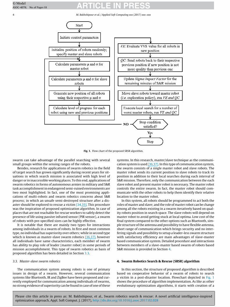
Fig. 1. Flow chart of thswarm can take advantage of the parallel searching with severalsmall groups within the sensing ranges of the robots.
Besides, research for applications of swarm robotics in the fieldof target search has grown significantly during recent years for sit-uations in which search mission is associated with high level ofdanger or in inaccessible working places. To this end, applications ofswarm robotics in forms of autonomous armies in military and S&Rtask accomplishment in endangered semi-ruined environments aretwo most highlighted. In fact, one of the most promising appli-cations of multi-robots and swarm robotics concerns about S&Rprocess; in which an unsafe semi-destroyed structure after a dis-aster should be explored to rescue a victim [34,35]. This procedurewas the inspiration of proposed optimization algorithm. In case ofplaces that are not reachable for rescue workers to safely detect thepresence of life using passive infrared sensor (PIR sensor), a swarmof robots with pre-specified sizes can be highly effective.
It is notable that there are mainly two types for interactionsamong individuals in a swarm of robots. In first and most commontype, no individual has superiority over others; while in second typewhich is known as master-slave swarm robotics [36,37], howeverall individuals have same characteristics, each member of swarmhas ability to play role of leader (master robot) in some periods ofmission accomplishment. This type of swarm robotics as basis ofproposed algorithm has been detailed in Section 3.3.
3.3. Master-slave swarm robotics
The communication system among robots is one of primary
Please cite this article in press as: M. Bakhshipour, et al., Swarm rooptimization approach, Appl. Soft Comput. J. (2017), http://dx.doi.org
issues in design of a swarm. However, several communicationsystems like Bluetooth, IR and ZigBee have been proposed and cur-rently employed for communication among individuals of swarms,no strong evidence of superiority can be found in case of one of these
osed SRSR algorithm.
systems. In this research, master/slave technique as the communi-cation system is used [36,37]. In this type of communication system,the swarm consists of a single master robot and slave robots. Themaster robot sends its current position to slave robots to track itsposition in addition to their local searches during each interval ofS&R mission. Therefore, only the communication between the eachslave robot and present master robot is necessary. The master robotcontrols the entire swarm. In fact, the master robot should com-municate with the other robots to help them identify their relativelocation to the master robot.
In this system, all robots should be programmed to act both theroles of master and slave; and the role of master robot can be changeamong all the robots existing in a swarm iteratively based on qual-ity robots position in search space. The slave robots will depend onmaster robot to avoid getting stuck at local optima. Low cost of thefinal system compared to the other options such as Bluetooth, sim-ple structure of the antenna and possibility to have flexible antenna,short range of communication which brings security and no inter-fering signals and possibility to setup a leader-less swarm structurewith satisfactory efficiency are main advantages of slave-masterbased communication system. Detailed procedure and interactionsbetween members of a slave-master based swarm of robots basedS&R mission is provided in Section 4.
4. Swarm Robotics Search & Rescue (SRSR) algorithm
In this section, the structure of proposed algorithm is described
botics search & rescue: A novel artificial intelligence-inspired/10.1016/j.asoc.2017.02.028
based on cooperative behavior of a swarm of robots to searcha victim in a post-disaster location. Flowchart depicted in Fig. 1shows the procedure of algorithm implementation. As like as otherevolutionary optimization algorithms, it starts with creation of a

ARTICLE IN PRESSG Model
ASOC-4078; No. of Pages 18
M. Bakhshipour et al. / Applied Soft Computing xxx (2017) xxx–xxx 5
n pro
P
Vv
WaN
tab
nu
Fig. 2. Normal distributio
population of robots. In next step, robots should be distributedin catastrophe areas. Then, they start to search and appraise areanear their position and by utilization of high-tech sensors mountedon robots for attaining specified vital signs of the victim, mostlyhuman. Based on data gathered by robots, the superior individualamong the swarm plays role of the master robot and should con-duct group to promoted situations; while it is mandatory for otherrobots to perform as the slaves. In such the condition, quality of arobot position is completely related to its sense of environment and,subsequently its ability to track vital signs of victim. It is noteworthythat all robots in a swarm have similar construction specifications,and therefore their abilities to response to environmental signalsand to analyze the received information are identical as well. Dur-ing the search and rescue (S&R) mission, with leadership of therobot named master due to highest peripheral perception from vic-tim, three policies including 1) Accumulation: gathering of slaverobots in a position near the position of master robot, 2) Explo-ration: search of distance between slave and master robots by slaverobots and, 3) Local search: search of specified number of robotssurrounding the position of master robot should be accomplished.
As opposed to individuals in natural swarms, semi-advancedrobots in a homogeneous group have a limited ability to recordprevious steps. This characteristic assists members to return to pre-vious positions if they don’t reach a favorable position during theperiod of mission accomplishment. However, due to the mentionedhardware limitations of robots in a swarm with large number ofmembers which are designed for a coherent behavior in a rescuemission, the chip design of robots will not permit them to recordmore than one or two previous steps. Besides, the robustness ofswarm robotic systems comes from the implicit redundancy inthe swarm. This redundancy allows the swarm robotic system todegrade peace-fully making the system less prone to catastrophicfailures. For instance, swarm robotic systems can create dynamiccommunication networks in the battlefield. The first hypothesisfor these swarms assumes that each individual owns a unique IDfor communication and cooperation. Such networks can enjoy therobustness achieved through re-configuration of the communica-tion nodes when some of the nodes are hit by enemy fire. However,there are some limitations for swarm like central automatic controlby which slave robots are restricted to communicate solely withmaster robot. While a slave robot reaches a position better thanthat of master robot, it should guide swarm for rest of mission asthe master robot; while prior master will play role of a slave robot.In fact, they should exchange their duties and responsibilities of
Please cite this article in press as: M. Bakhshipour, et al., Swarm rooptimization approach, Appl. Soft Comput. J. (2017), http://dx.doi.org
S&R mission for remaining minutes ahead. The rest of paper illus-trates how S&R mission is modeled based on swarm robotics foroptimization task.
bability density function.
4.1. Generating initial swarm of robots
In order to obtain a global solution of an optimization problem,the first step is to form decision variables of problem as an array.In different codifications of optimization algorithms, this array hasbeen called with different names. For instance, it is named as chro-mosome, social-political position of a country and habitat in GA, ICAand COA, respectively. In the proposed algorithm, vector of decisionvariables is called robot position. In an optimization problem withNvar decision variables, each initial solution is composed of an arraywith dimension 1 × Nvar shows the position of a robot in search area.This position is defined by Eq. (1):
ositionirobot = [x1, x2, ...., xNvar ] , i = 1,2, , ...., Nrobots (1)
ariables x1, x2, ...., xNvar can be floating point numbers. Value ofictim’s vital signs (VVS) monitored by each robot is defined by Eq.
(2):
VVS = f(
Positionirobot
)
= f ([x1, x2, ...., xNvar ]) , i = 1,2, , ...., Nrobots (2)
here f is referred to optimization function. Considering Nrobots
s number of robots in initial swarm, a matrix with dimension of
robots × Nvar is generated as initial population of robots. In a solu-ion search space with maximum and minimum limits of Varmax
nd Varmin, respectively; initial position of a robot can be obtainedy Eq. (3):
Positionrobot = Urnd(
Varmin, Varmax, Varsize
)
(3)
Function Urnd generates an array of random floating-pointumbers from continuous uniform distribution with lower andpper endpoints specified by Var
minand Varmax , respectively; and
Varsize = 1 × Nvar.As mentioned, after generating initial solutions and evaluating
of initial population, master and slave robots are determined basedon fitness of VVSs. Then, three main policies of algorithm includingaccumulation, exploration, and local search are implemented asfollows:
4.2. Accumulation
During the first policy of algorithm, all slave robots should moveto a position near the position of the master robot aiming at ame-liorating its current sense of VVS. This accumulation nearby theposition of best robot is implemented with random movementsand by utilizing normal probability distribution function (PDF). The
botics search & rescue: A novel artificial intelligence-inspired/10.1016/j.asoc.2017.02.028
probability density of normal distribution is given by Eq. (4):
y = f [x|�,�] =1
�√
2�e
−(x−�)2
2�2 (4)

ARTICLE IN PRESSG Model
ASOC-4078; No. of Pages 18
6 M. Bakhshipour et al. / Applied Soft Computing xxx (2017) xxx–xxx
robot
en
etlp
Wiamwtci
4
�
r
Si
r
4
s
− Pos
t[M](j
Fig. 3. Movement of slave robot toward master
Here parameter � is mean or expectation of distribution andparameter � is its standard deviation with its variance then �2.A random variable with a Gaussian distribution is said to be nor-mally distributed and is called a normal deviate. If �= 0 and � = 1,the distribution is called the standard normal distribution denotedbyN (0,1). As it can be seen in Fig. 2, with variations of two param-ters � and �, different ranges of PDF based random floatingumbers can be obtained.
The master robot transmits its current position to slave robotsmploying predesigned communication systems like Bluetoothechnology, global positioning system (GPS) and etc. as an accumu-ation command. Subsequently, slave robots start to change theirosition toward the position of the master robot.
Comparing normal PDF to some other well-known PDFs likeeibull, Gamma or Pareto, it should be mentioned that the most
mportant aspect about these functions is that these are skewednd asymmetric. These distribution functions are mostly used toodel phenomena in which generated points should be distributedith high probabilities at first/ending stages of phenomenon. On
he contrary, the great power of the normal distribution is that theoncept of Master-Slave in a swarm of robots can be transformednto a normal distribution via Central Limit Theorem [38]. More-
over, it also serves a physical manifestation. Due to fact that thereis no certain justification about superiority of movement direction
for an individual in a swarm of robots with limited level of intelli-gence, especially during first iterations, robots should explore bothdirections with same probability to maintain diversity and also toprevent plighting in local minimums. Using Weibull, Gamma orPareto distributions, probability to search on one direction towardthe master robot will be dominant and logically, because of highconvergence toward local minimums during first iterations of algo-
�irobot[S]
= SCF i ×(
Positionrobot[M]
+r2 × Positionirobot[S]
(j) |(Position
robo
Please cite this article in press as: M. Bakhshipour, et al., Swarm rooptimization approach, Appl. Soft Comput. J. (2017), http://dx.doi.org
rithm execution, an extensive exploration of search space for globaloptimum cannot be achieved.
Values � and � for master and slave robots can be obtained asfollows:
by the accomplishment of accumulation policy.
.2.1. Calculation of parameters � and � for master robot
As aforementioned, master robot calls slave robots up to its cur-rent position with aim of directing population to location with themaximum likelihood of victim presence. As long as slave robots areaccumulating in position of master robot, it starts a local searchnearby the stated position. In fact, by execution of such the search,master robot tries to improve its situation during period otherrobots are moving toward position in which maximum VVS hasbeen found. Considering C1 as first control parameter, values� and
for master robot are defined by Eqs. (5) and (6), respectively:
�robot[M] = r (5)
�robot[M] =(
1 + (−1)Eit+1 × �robot[M]
/(
max(
0, (−1)Eit+1)
× (1 − C1) + 1))
× Positionrobot[M](6)
is a random number within [0,1], Eit denotes elapsed time of&R mission in SRSR terminology, refers to number of iterationsn algorithm codification and Position
robot[M]is position of master
obot.
.2.2. Calculation of parameters � and � for slave robots
During implementation procedure of accumulation policy, alllave robots should be relocated by their own parameters� and �.
Parameters for slave robots are defined by Eqs. (7) and (8):
itionirobot[S]
)
)−Positionirobot[S]
(j))
<0.05, i = 1, ...., Nslaves; j = 1, ...., Nvar
(7)
�irobot[S]
= C1 × Positionrobot[M]
+ (1 − C1) × Positionirobot[S]
, i = 1, ...., Nslaves (8)
SCFi is a correction factor for parameter � corresponding to slaverobot i. Calculation method of SCF value has been detailed in Section4.2.5. The schematic representation for calculation procedure ofnew position of a slave robot by executing accumulation policy inrelation to master robot is shown in Fig. 3. It should be mentionedthat the location
(
�p1,�p2,�p3
)
enjoys maximum likelihood to
botics search & rescue: A novel artificial intelligence-inspired/10.1016/j.asoc.2017.02.028
be chosen as the next position of slave robot. However, based onthe variance obtained for each of the axes which refer to decisionvariables, the locations near the location of master robot might beproportionally chosen with lower probabilities.

ING Model
A
Soft C
4
l
N
4
eebstetartoTrb
)
prictspfii
tfi
4
t
Ss
[
d
V
(
a
ARTICLESOC-4078; No. of Pages 18
M. Bakhshipour et al. / Applied
.2.3. Generating new positions
In this section, new position of master and slave robots by uti-izing parameters � and � corresponding to each robot should be
determined.
New Positionrobot[i] = Nrnd(
�robot[i], �robot[i])
, i =Master, Slaves(9)
Function Nrnd generates an array of random floating pointnumber from normal PDF with mean parameter � and standarddeviation parameter � obtained from two previous sections. It isnoteworthy; this equation is valid to determine new position forboth master and slave robots. In order to bound new obtainedpositions in range of search space, following equations are utilized:
New Positionrobot[i] (j) = max(
Varmin (j) ,New Positionrobot[i] (j)
) , i =Master, Slaves; j = 1, ...., Nvar (10)
New Positionrobot[i] (j) = min(
Varmax (j) ,New Positionrobot[i] (j)
) , i =Master, Slaves; j = 1, ...., Nvar (11)
ew VVSrobot[i] = f(
New Positionrobot[i]
)
, i =Master, Slaves (12)
.2.4. Progress assessment
In nature, there are a large number of creatures with somelements of cooperative behaviors. In animal communities, manympirical evidences suggest that performance of a cooperativeehavior may not be desirable in a period of time and it was impos-ible to return to previous situation. Lack of a temporary memoryo record accurate previous situation and time variant features ofnvironmental elements are two key factors for occurrence of theseypes of events. However, such the happenings are not mostly prob-ble in artificial intelligence territory. As an illustration, a simpleobot in a S&R swarm with moderate functionality which has abilityo record one previous step can change its current position to previ-us one if desired improvements are not achieved in new position.his capability has been considered for rescuer robots in swarmobotics. Mathematic formulation of this characteristic is definedy Eq. (13):
if NewVVSjrobot[i]
< VVSjrobot[i]
, i =Master, Slaves; j = 1, ...., Nvar
VVSjrobot[i]
= NewVVSjrobot[i]
Positionrobot[i] = NewPositionrobot[i]
end
(13
However, it should be mentioned that by implementation of thisolicy during every minute of the S&R mission for all robots, theyapidly gather at a local optimum location and algorithm will losets diversity factor gradually in search process. Therefore, after relo-ation of robots to their new position and sorting them based onheir new VVS quality, one of values 50% or 100% of populationhould be selected randomly by algorithm. If 50% is selected, robotopulation should be divided to two groups. Then, robots in therst group which enjoy higher VVS values are permitted to reside
n new positions, if NewVVSrobot
< VVSrobot
; otherwise, they aresubject to return to previous positions. Whereas, members of thesecond group should reside in new positions without any consid-eration of improvement in NewVVS to maintain diversity of wholehe population. If value 100% is selected, method employed for therst group should be utilized for all members of population.
Please cite this article in press as: M. Bakhshipour, et al., Swarm rooptimization approach, Appl. Soft Comput. J. (2017), http://dx.doi.org
.2.5. Calculation of SCFAfter settling of robots at their new position at the end of each
ime interval of S&R mission, SCF value should be modified for
PRESSomputing xxx (2017) xxx–xxx 7
coming one minute (refers to next iteration in algorithm imple-mentation) based on VVS change of robots in current iteration. Thatis the robot which enjoys highest VVS change compared to previ-ous one minute should be considered as basis for modification ofrobots movement in coming one minute of S&R mission. Calculationprocedure of SCF is detailed in the following steps:
Step 1: Let SIF = 6 as an initial value for the first iteration (algo-rithm is not sensitive to this value, because value of this temporaryvariable will be modified iteratively).
Step 2: Calculate SCFi = SIF × ri, i = 1, ...., Nrobots; ri is random num-ber within [0,1] corresponding to robot i.
Step 3: Calculate VVSiMovement = VVSirobot
− NewVVSirobot
, i =1, ...., Nrobots
Step 4: Select index i which refers to robot enjoysmaximumVVSMovement
Step 5: CalculateSIF =(
1 +(
max
(
Varmax − Varmin,
))
× r)
×
CFmax; SCFmax is value of SCF corresponding to robot which iselected in step 4.
Step 6: Limit SIF value obtained in previous step within
0,max
(
Varmax
)]
, derived from six sigma theory [39].
Step 7: Go step 2 for new iteration.It is noteworthy variable VVSiMovement in step 3 should be
etermined before implementation of “Section 4.2.4 progressassessment” in which variables Position and VVS are updated basedon improvements of robots; otherwise, it is probable about someof robots to return to their respective position if new positions arenot more justified in term of VVS
robotvalue.
4.3. Exploration
Exploration policy is another main operator of proposed algo-rithm by which slave robots are allowed to search spaces aroundthemselves in a direct path toward/backward master robot. Newposition of slave robots by execution of exploration policy can beobtained by Eq. (14):
NewPositionirobot[S]
= r × Positionirobot[S]
+GB×(
Positionrobot[M]
− Positionirobot[S]
)
×MF, i = 1, ...., Nslaves
(14)
ariable GB = ±1 is selected randomly and vector of movement factor
MF) is calculated bymax
(
1, |Positionrobot[M]
− Positionrobot[WS]
|)
t the end of each iteration; here index WS refers to slave robotwith the worst VVS. Parameter MF can control convergence speedand accuracy of search at different intervals of algorithm execu-tion. This movement is shown in Fig. 4. As it can be seen, a randompercent of current position of a slave robot is added to/subtractedfrom a factor of direct path from position of slave robot to position ofmaster robot. In fact, the first term of exploration equation changesdistance and initial angle of position of a slave robot with respect tomaster robot (first step), randomly; while the second term of explo-ration equation moves position of slave robot toward/backwardmaster robot (second step). After creating new position of slaverobot, all steps proposed in Section “4.2.4 progress assessment”should be implemented to determine optimal position of slaverobots in current one minute of S&R mission.
4.4. Local search
botics search & rescue: A novel artificial intelligence-inspired/10.1016/j.asoc.2017.02.028
In this policy, a specified number of robots which have lowestqualities perform as worker robots. These robots are assigned to alocal search around the position of master robot. In fact, this pol-icy is an extra accurate search by which worker robots, that refer

ARTICLE IN PRESSG Model
ASOC-4078; No. of Pages 18
8 M. Bakhshipour et al. / Applied Soft Computing xxx (2017) xxx–xxx
f expl
N
eo
4
N bot[M
bot[M
pr
4
fN
P
cas
4
i
i
m0
5
atptsh
Fig. 4. Two steps o
to low quality solutions in optimization algorithm, are permittedto improve their position. However, residing of worker robots atnew positions is possible only when they reach a position bet-ter than position of robot enjoying second rank. Otherwise, theyshould return to the previous position after an unsuccessful search.In order to implement such an expression, some arithmetic opera-tors with elementary operations have been employed to determinethe new position of worker robots as follows:
4.4.1. Round operator
NewPosition1robot[W]
= sign{
round+(
|Positionrobot[M]|)}
robot[M](15)
ewPosition2robot[W]
= sign{
round−(
|Positionrobot[M]|)}
robot[M](16)
Operators round+ (x)/round− (x) round elements of x to near-st integers greater than/less than or equal to x, respectively; andperator sign{ω} reflects signs of to ω element by element.
.4.2. Exponential operator
ew Position3robot[W]
= sign{
Int{
Positionrobot[M]
}
+(
Fra{
Positionro
New Position4robot[W]
= sign{
Int{
Positionrobot[M]
}
+(
Fra{
Positionro
Functions Int{
�}
and Fra{
�}
return integer and fractionalarts of elements of �, respectively. Parameters e1 and e2 are twoandom integers within [2,4].
.4.3. Combined operator
This operator is retrieved from crossover policy in GA. Inact, new position of worker robot 5 is a combination ofewPosition3
robot[W]and NewPosition4
robot[W]with random shares of
1 and P2, respectively; while, P1 + P2 = 100%.
New Position5robot[W]
=[[
P1%(
NewPosition3robot[W]
)] [
P2%(
NewPosition4robot[W]
)]]
(19)
Please cite this article in press as: M. Bakhshipour, et al., Swarm rooptimization approach, Appl. Soft Comput. J. (2017), http://dx.doi.org
It is noteworthy such implementation is accomplished about aertain number of decision variables, not all variables of positionrray to prevent sudden chaotic changes in position of obtainedolutions.
oration procedure.
]
})1e1}
robot[M](17)
]
})e2}
robot[M](18)
.5. Control parameters
Control parameters of algorithm are as follows:
i Mu factor [C1]: controls mean values for master and slave robots.This parameter controls dominance degree of the master robot.
ii Movement factor [C2]: determines movement pace of robotsduring exploration policy
ii Sigma factor [C3]: determines level of divergence of the slaverobots from master robot.
v Sigma limit [C4]: limits value of sigma factor
In this algorithm, control parameters C2, C3 and C4 are auto-atically tuned; while C1 should be adjusted by user within [0.5,
.85].
. Case study and results
In this paper, the effectiveness of the presented method has beenssessed in two scenarios. For first scenario, a number of standardest functions have been employed; while, in second scenario, theroposed method has been applied to obtain optimum schedulingable for medium-scale (10 unit system) to large-scale (100 unitystem) thermal electric power generating systems. The proposedeuristic algorithm has been implemented on an Intel
®CoreTM
i5–460 M Processor (3 M Cache, 2.53 GHz).
5.1. Scenario 1: standard benchmark functions
For this scenario, the proposed method has been applied to aset of unimodal (F1–F10; for scales of small (D1), medium (D2) andlarge (D3)) and multimodal (F11–F14) standard benchmark func-
botics search & rescue: A novel artificial intelligence-inspired/10.1016/j.asoc.2017.02.028
tions. These functions have been detailed in Tables 2 and 3. Theproposed algorithm has been run for 50 times. In order to guar-antee a fair comparison among different algorithms and to avoidconsideration of execution time as the comparison index (because

ARTICLE IN PRESSG Model
ASOC-4078; No. of Pages 18
M. Bakhshipour et al. / Applied Soft Computing xxx (2017) xxx–xxx 9
Fig. 5. Multimodal functions with a few local minima (f11: Six Hump Camel Back and f12: Himmelblau).
local
dmtimapw
f
focmf
x
v
x
Fig. 6. Multimodal functions with many
ifferent qualities of codification for a same problem formulationay result in different execution times), maximum number of func-
ion evaluations (NFE) is considered as stop criterion of algorithmmplementation. NFE parameter has been set to 5000 in case of uni-
odal and 10000 in case of multimodal benchmark functions. Forll other algorithms, the maximum NFE has been set to that of theroposed algorithm. Multimodal functions include two functionsith a few local minima (F11 and F12 depicted by Fig. 5) and two
functions with many local minima (F13 and F14 depicted by Fig. 6).In implementation procedure of algorithm, stop criterion is
defined by Eq. (20):
end.it(robot[M]) − globalmin ≤ StC (20)
end.it(robot[M]) is cost of the best obtained solution at last iterationf algorithm and StC is stopping criterion of the algorithm, when itonverges into 10−6 and 10−3 tolerance in cases of unimodal andultimodal functions, respectively. Mean and standard deviation
or obtained results are calculated by Eq. (21):
Std.dev =
(
1
n
n∑
i=1
(xi − x)2
)12
(21)
i is vector of solutions resulted by runs of program and x is mean
Please cite this article in press as: M. Bakhshipour, et al., Swarm rooptimization approach, Appl. Soft Comput. J. (2017), http://dx.doi.org
alue of solutions:
¯ =1
n
n∑
i=1
xi (22)
minima (f13: Hansen and f14: Shubert).
Obtained results including best (min), arithmetic average(mean), worst (max) and standard deviation (Std. dev.) after 50independent executions of proposed SRSR optimization algorithmhave been compared with those of TLBO, ABC, ICA, BBO, GSA, PSOand DE in Tables 4–6 for dimensions D1-D3, respectively. As itcan be deduced from Table 4, proposed SRSR methodology showsthe best performances among presented methods; while the worstperformance is related GSA. ABC and ICA enjoy relatively equal per-formances and also weaker performances compared to SRSR andTLBO. Obviously, proposed algorithm demonstrates its superior-ity and efficiency in cases of reaching global solution and lowerstandard deviations. Moreover, in case of max (worst) solution, pro-posed algorithm has shown its excellence in comparison task for allbenchmark functions. Although, BBO presents a better performancethan GSA, solutions obtained by executions of these algorithms donot enjoy expected quality to be comparable with other algorithms.Moreover, considering little changes in ranking, PSO and DE providesolutions relatively as similar as TLBO in most of the cases.
Referring to Table 5 and 6, superiority of SRSR method can behighly demonstrated by comparison of obtained results with thoseof literature review for medium and large scale unimodal problems.
Convergence curves of the proposed algorithm versus NFE fordifferent benchmark functions are compared with those of ABC,
botics search & rescue: A novel artificial intelligence-inspired/10.1016/j.asoc.2017.02.028
TLBO, ICA, BBO and GSM in Fig. 7. In the case of single objectivefunctions, superiority of SRSR over other algorithms in term of thesolution quality is evident; however such the superiority cannot beobserved for all benchmark functions in term of convergence pace.

ARTICLE IN PRESSG Model
ASOC-4078; No. of Pages 18
10 M. Bakhshipour et al. / Applied Soft Computing xxx (2017) xxx–xxx
Table 2
Standard unimodal test functions.
Func Definition Interval Global minimum Dimension
D1 D2 D3
F1 f (x) =
N∑
i=1
x2i
[−100,100] 0 10 50 200
F2 f =
D∑
i=1
[100(xi2 − xi+1)
2 + (1 − xi)2] [−10,10] 0 2 50 200
F3 f (x, y) = y sin(4x) + 1.1x sin(2y) [−10, 10] −19.8623 2 – –
F4 f = 10n+
n∑
i=1
(xi2 − 10 cos(2�xi)) [−5.12,5.12] 0 3 50 200
F5 f (x) = −20 exp(−0.2
√
√
√
√1
30
D∑
i=1
xi2) − exp( 130
D∑
i=1
cos 2�xi) [−30,30] 8.8818e-16 10 50 200
F6 f (x) =
N∑
i=1
(x2i
+ xi) cos(xi) [−10,10] −100.22375 × D 2 50 200
F7 f (x, y) = x sin(4x) + 1.1y sin(2y) [−10,10] −18.5547 2 – –
F8 f (x) =
N∑
i=1
(|xi| − 10 cos(√
|xi|) [−10,10] −10 × D 10 50 200
F9 f (x) = 0.5 +sin2(
√
(x21+x2
2))−0.5
1+0.001(x21+x2
2)
[−10,10] 0 2 – –
F10 f (x) = 1 +
N∑
i=1
x2i
4000 −
N∏
i=1
cos(xi√i) [−10,10] 0 10 50 200
Table 3
Standard multimodal test functions.
Func Definition Interval Global minimum Global peaks
F11 f (x) =(
4 − 2.1x21
+x4
13
)
x21
+ x1x
2+(
−4 + 4x22
)
x22
x1 ∈ [−1.9, 1.9] x2 ∈ [−1.1, 1.1] −1.03162 2
F12 f (x) =(
x21
+ x2
− 11)2
+(
x1
+ x22
− 7)2
x1 ∈ [−6, 6] x2 ∈ [−6, 6] 0 4
F13 f (x) =
(
5∑
i=1
i cos ((i− 1) x1 + i)
)
×
(
5∑
j=1
j cos ((j + 1) x2 + j)
)
x1 ∈ [−10, 10] x2 ∈ [−10, 10] −176.541 18*
F14 f (x) =
(
5∑
i cos ((i+ 1) x1 + i)
)
×
(
5∑
j cos ((j + 1) x2 + j)
)
x1 ∈ [−10, 10] x2 ∈ [−10, 10] −186.730 18*
i=1 j=1
* indicates minimum number of peaks for 2D function.
It should be mentioned that convergence quality of algorithms iscompletely related to features of benchmark functions. Needlessto say, level of adaptability of an optimization algorithm cannot bedetermined by applying to a limited number of problems. As anillustration, GSM algorithm does not provide quality solutions inmost of cases, while its convergence speed surpasses that of otheralgorithms for function F1.
In case of multimodal functions (F11–F14), results of compari-son of SRSR with other algorithms based on success times (numberof runs in which all global peaks have been found), mean (aver-age final value of all runs of algorithm) and average number ofoptima found (the average number of peaks found over 50 runswith StC = 1 × 10⁻³) are detailed in Table 7. As it can be seen,maximum number of success times has been obtained by SRSR.
Please cite this article in press as: M. Bakhshipour, et al., Swarm rooptimization approach, Appl. Soft Comput. J. (2017), http://dx.doi.org
Considering more challengeable feature of multimodal benchmarkfunctions compared to unimodal functions, success rates for mul-timodal functions are not as high as unimodal functions. In caseof multimodal functions F11–F14, TLBO and ABC have better per-
formances than ICA in most of cases. It is noteworthy, with theincrement of complexity of benchmark functions from F11 to F14,quality of solutions are reduced. As an illustration, average optimafound by SRSR for the function F11 is 2 where there are two globalpeaks (100% success rate); However, there are 18 global peaks forfunction F14 and the best average optima found is 16.18 by SRSR(89.9% success rate). Such the statement is true about number ofsuccess times and mean values as well. Results obtained by BBO andGSA implementations show none of them are capable of compar-ing with other algorithms. However, TLBO has approximately equalperformances to SRSR about functions F11 and F12, superiorities ofproposed algorithm are obvious in cases of benchmark functionsF7 and F8 where complexities of test functions are increased.
botics search & rescue: A novel artificial intelligence-inspired/10.1016/j.asoc.2017.02.028
5.2. Scenario 2: practical power system problem
In order to evaluate the quality of the proposed technique fora practical problem, unit commitment as one the most important

ARTICLE IN PRESSG Model
ASOC-4078; No. of Pages 18
M. Bakhshipour et al. / Applied Soft Computing xxx (2017) xxx–xxx 11
Table 4
Comparison of best obtained solutions from different algorithms (unimodal function); dimension: D1.
ABC TLBO ICA BBO GSA PSO DE SRSR
F1 Min (best) 0.0368 3.24 × 10−06 51.6464 4.4543 5.8254 4.16 × 10⁻¹⁴ 41.82 × 10−09 0
Mean 0.4282 9.34 × 10−05 196.9432 17.3496 15.2565 8.99 × 10⁻¹² 4.57 × 10−08 0
Max (worst) 1.4496 0.0011 606.8374 52.3666 24.0362 1.83 × 10⁻¹⁰ 2.73 × 10−07 0
Std. dev. 0.3499 1.82 × 10−04 117.6103 10.7962 4.0361 2.70 × 10⁻¹¹ 5.95 × 10−08 0
F2 Min (best) 5.61 × 10−07 6.83 × 10−05 1.06 × 10−05 0.0306 0.0086 3.13 × 10⁻¹⁶ 1.82 × 10⁻¹⁸ 0
Mean 0.0017 2.42 × 10−02 0.0272 1.1487 0.349 374 × 10−09 1.96 × 10−09 0
Max (worst) 0.0177 0.1654 0.5372 5.5865 1.1296 4.95 × 10−08 7.14 × 10−08 0
Std. dev. 0.0035 0.0328 0.0787 1.3068 0.2913 1.03 × 10−08 1.07 × 10−08 0
F3 Min (best) −19.8623 −19.8623 −19.8623 −19.7337 −19.7744 −19.8623 −19.862 −19.8623
Mean −19.8623 −19.8621 −19.786 −18.3463 −18.5486 −17.0653 −19.337 −19.8623
Max (worst) −19.8623 −19.8582 −18.5916 −16.8589 −17.4261 −11.6434 −17.494 −19.8622
Std. dev. 4.48 × 10⁻¹⁰ 5.71 × 10−04 0.3048 0.6638 0.5188 1.9560 0.96656 1.69 × 10−06
F4 Min (best) 1.99 × 10−06 0 2.95 × 10−05 0.011 1.0318 0 0 0
Mean 0.3137 2.54 × 10⁻¹³ 0.2013 0.6115 4.2586 1.3730 0 0
Max (worst) 1.6941 5.01 × 10⁻¹² 1.0074 1.7147 7.7237 4.9748 0 0
Std. dev. 0.4339 8.80 × 10⁻¹³ 0.3833 0.4815 1.5559 1.3164 0 0
F5 Min (best) 0.1132 0.0027 3.7334 1.4843 4.8953 5.32 × 10−08 1.38 × 10−05 8.88 × 10⁻¹⁶
Mean 0.4015 0.0451 6.5576 2.8951 6.1779 0.1715 1.28 × 10−04 8.88 × 10⁻¹⁶
Max (worst) 1.3313 0.955 10.5058 4.7718 7.3042 1.6462 1.73 × 10−03 8.88 × 10⁻¹⁶
Std. dev. 0.2694 0.1332 1.2746 0.599 0.5294 0.4344 2.49 × 10−04 0
F6 Min (best) −200.4475 −200.4475 −200.4475 −200.4471 −200.4395 −200.4475 −200.4475 −200.4475
Mean −200.0689 −200.4475 −198.5618 −199.9672 −199.0868 −150.7990 −197.6926 −200.4474
Max (worst) −181.5918 −200.4475 −181.5918 −198.2014 −193.2686 −89.8412 −181.5918 −200.4470
Std. dev. 2.6664 1.56 × 10⁻¹² 5.71 0.5861 1.3386 42.3979 4.6158 1.08 × 10−04
F7 Min (best) −18.5547 −18.5547 −18.5547 −18.5544 −18.5516 −18.5547 −18.5547 −18.5547
Mean −18.5521 −18.5547 −18.5547 −18.4316 −18.3571 −16.6552 −18.5547 −18.5547
Max (worst) −18.4758 −18.5547 −18.5547 −16.9746 −17.8192 −10.3993 −18.5547 −18.5545
Std. dev. 0.0126 1.73 × 10−07 1.31 × 10−07 0.2269 0.1867 2.0012 1.79 × 10⁻¹⁴ 4.73 × 10−05
F8 Min (best) −76.2009 −80.2417 −70.9271 −87.5371 −45.7483 −76.7780 −80.574 −100
Mean −65.3395 −73.1429 −59.3421 −77.647 −39.1211 −65.9410 −67.848 −100
Max (worst) −59.7662 −67.8236 −35.7792 −71.1918 −32.0331 −61.2966 −60.995 −100
Std. dev. 3.4832 2.8901 8.1086 3.8414 3.5161 4.2108 −60.995 0
F9 Min (best) 0 1.24 × 10−04 3.98 × 10⁻¹² 2.90 × 10−05 3.60 × 10−05 0 0 0
Mean 9.46 × 10⁻¹⁰ 0.0163 8.30 × 10−03 0.0402 0.0073 0.0161 2.02 × 10−03 0
Max (worst) 4.71 × 10−08 0.0406 0.0447 0.0445 0.0265 0.0447 4.47 × 10−02 0
Std. dev. 6.66 × 10−09 0.0106 1.73 × 10−02 0.0125 0.0066 0.0217 8.86 × 10−03 0
F10 Min (best) 4.40 × 10−04 6.34 × 10−05 0.9997 0.0168 0.3207 0 0.0309 0
Mean 0.1279 0.0334 1.0004 0.0579 0.5894 0.0399 0.1502 0
Max (worst) 0.4574 0.0456 1.0019 0.1129 0.7471 0.1229 0.3316 0
0.022
ppasi
rcft[
5
5
(o
U
H
T
Ii
C
taud
M
ocuu
Std. dev. 0.1069 0.0166 5.69 × 10−04
roblems in operation of electric power system is assessed. Thisroblem is a large-scale mixed integer problem (MIP) in which day-head power production scheduling of thermal generating unitshould be determined aiming at minimizing operating costs includ-ng fuel cost, start-up and shut-down costs.
This problem is subjected to some system (e.g. demand andeserve) and units (e.g. minimum on/off time, ramp up/down rates)onstrains. It is noteworthy due to large scale and non-convexeatures of this problem; it is a costly problem from computa-ional view point which has been investigated in many researches44–51].
.2.1. UC problem formulation
.2.1.1. Objective Function. The objective function of UC problemUCOF) for a generating system consisting N units and for T hoursf scheduling horizon can be formulated as:
COF = minimize (TC) (23)
Please cite this article in press as: M. Bakhshipour, et al., Swarm rooptimization approach, Appl. Soft Comput. J. (2017), http://dx.doi.org
ere:
C =T∑
t=1
N∑
i=1
[
Ci(
P(i,t).I(i,t))
+ ST(i,t).I(i,t).[1 − I(i,t−1)]]
(24)5
l
2 0.1001 0.0313 0.0574 0
(i,t) commitment state of unit i at time t, and fuel cost for generatorwith fuel cost coefficients ai, bi and ci is defined by Eq. (25):
i
(
P(i,t).I(i,t))
= ai + bi × P(i,t) + ci × P(i,t)2 (25)
Start-up costs can be expressed as an exponential or linear func-ion of the time [39]. In this paper, start-up costs are modeleds a two-valued (hot start/cold start) staircase function [44]. Fornit i with hot start-up cost (HSCi) and cold start-up (CSCi), time-ependent cost of start-up is defined by Eq. (26) [44]:
ST(i,t) =
{
HSCi, ifMDTi ≤ DTi ≤MDTi + CSHi
CSCi, ifDTi >MDTi + CSHi(26)
DTi is minimum down-time limit of unit i, CSHi is cold start hourf unit i, and DTi is the unit’s down time. Similarly, Shutdown costan be considered as a fix, staircase or exponential cost for eachnit per shut down. However, in this paper, the shut-down cost ofnits is not considered during simulation procedure.
botics search & rescue: A novel artificial intelligence-inspired/10.1016/j.asoc.2017.02.028
.2.1.2. Constraints. The PBUC problem is formulated subject to fol-owing system and unit constraints [46].
A. Unit constraints

Please cite this article in press as: M. Bakhshipour, et al., Swarm robotics search & rescue: A novel artificial intelligence-inspiredoptimization approach, Appl. Soft Comput. J. (2017), http://dx.doi.org/10.1016/j.asoc.2017.02.028
ARTICLE IN PRESSG Model
ASOC-4078; No. of Pages 18
12 M. Bakhshipour et al. / Applied Soft Computing xxx (2017) xxx–xxx
Table 5
Comparison of best obtained solutions from different algorithms (unimodal function); dimension: D2.
ABC TLBO ICA BBO GSA PSO DE SRSR
F1 Min (best) 20.9616 0.0770 90.4533 2.65 × 10³ 202.0650 86.7748 338.26 0
Mean 259.4144 1.2408 331.8823 4.32 × 10³ 300.4854 8.3405 685.04 0
Max (worst) 1013.7 5.9629 869.7397 6.20 × 10³ 628.7836 493.2527 1248.9 0
Std. dev. 248.9055 1.1920 168.0125 767.6956 65.5196 96.6024 229.03 0
F2 Min (best) 431.4416 49.0658 799.9275 1.21 × 10⁴ 7.15 × 10⁴ 156.6446 3075.6 48.5066
Mean 8.48 × 10³ 49.9723 1.93 × 10³ 2.60 × 10⁴ 1.61 × 10⁵ 330.3673 9507.8 48.7696
Max (worst) 1.16 × 10⁵ 52.8635 4.03 × 10³ 5.21 × 10⁴ 2.71 × 10⁵ 883.0405 26352 48.9163
Std. dev. 1.77 × 10⁴ 0.8572 857.8237 8.86 × 10³ 4.91 × 10⁴ 151.5299 5542 0.1051
F4 Min (best) 0 24.9020 130.1062 97.1867 478.2112 65.4286 327.76 0
Mean 61.4583 101.6300 231.9110 117.6285 520.0191 99.5531 417.87 0
Max (worst) 252.7431 195.3031 342.9199 152.6470 553.5434 151.2542 480.95 0
Std. dev. 85.4016 42.9534 48.3793 11.8371 17.0121 22.4923 30.229 0
F5 Min (best) 5.9047 0.0621 6.0671 8.7395 8.2637 2.7354 4.7953 8.88 × 10⁻¹⁶
Mean 9.6925 0.2186 9.3658 10.1661 9.1511 4.5972 7.6771 8.88 × 10⁻¹⁶
Max (worst) 14.6906 0.4458 17.2838 11.6550 9.7827 7.6744 20.126 8.88 × 10⁻¹⁶
Std. dev. 2.1077 0.0935 2.5389 0.5837 0.3446 1.0973 3.0628 0
F6 Min (best) −4236.7 −4695.8 −3018.2 −4621.7 −1181.9 −2881.8 −4702.4 −4813.2
Mean −3845.1 −4545.1 −2529.5 −4445.5 −806.6711 −2219.7 −4473.6 −4681.6
Max (worst) −3490.0 4344.4 −1936.4 −4222.2 −539.5142 −1602.1 −4086.1 −4480.3
Std. dev. 183.5911 81.2469 218.2588 79.4057 134.3862 285.28 115.3663 62.73
F8 Min (best) −316.7334 −299.1715 −336.5846 −318.0996 −115.5267 −350.1117 −184.01 −500
Mean −289.7390 −276.2601 −295.9097 −298.1003 −90.9463 −331.5742 −129.29 −500
Max (worst) −249.4120 −249.5225 −184.8459 −281.6284 −64.5994 −317.5358 −82.62 −500
Std. dev. 15.6372 11.4651 36.8068 7.5289 11.6338 8.5092 25.41 0
F10 Min (best) 0.0288 3.24 × 10−05 0.0278 0.5816 0.9832 0.0031 0.1020 0
Mean 0.1971 3.14 × 10−04 0.870 0.7703 1.0399 0.0304 0.2985 0
Max (worst) 0.7102 0.0012 0.1915 0.9054 1.0546 0.1073 0.8113 0
Std. dev. 0.1194 2.34 × 10−04 0.3888 0.0694 0.0117 0.0218 0.1604 0
Table 6
Comparison of best obtained solutions from different algorithms (unimodal function); dimension: D3.
ABC TLBO ICA BBO GSA PSO DE SRSR
F1 Min (best) 1.37 × 10⁵ 0.6033 4.18 × 10⁴ 1.50 × 10⁵ 4.88 × 10³ 10103 89361 0
Mean 1.83 × 10⁵ 2.7282 5.78 × 10⁴ 1.74 × 10⁵ 8.91 × 10³ 15292 1.22 × 10⁵ 0
Max (worst) 2.32 × 10⁵ 7.5115 7.91 × 10⁴ 1.93 × 10⁵ 1.39 × 10⁴ 22349 1.63 × 10⁵ 0
Std. dev. 2.42 × 10⁴ 1.4664 8.66 × 10³ 9.53 × 10³ 1.98 × 10³ 2397.4 17172 0
F2 Min (best) 3.49 × 10⁶ 200.1324 5.16 × 10⁵ 4.16 × 10⁶ 4.23 × 10⁵ 41095 2.68 × 10⁶ 198.5736
Mean 7.09 × 10⁶ 203.7160 9.23 × 10⁵ 5.13 × 10⁶ 6.40 × 10⁵ 74358 4.07 × 10⁶ 198.8343
Max (worst) 1.06 × 10⁷ 212.1350 1.82 × 10⁶ 6.49 × 10⁶ 1.27 × 10⁶ 134610 5.79 × 10⁶ 198.8995
Std. dev. 1.56 × 10⁶ 2.8224 2.71 × 10⁵ 4.67 × 10⁵ 1.38 × 10⁵ 18740 8.33 × 10⁵ 0.0603
F4 Min (best) 1.46 × 10³ 18.5455 1.34 × 10³ 1.48 × 10³ 1.90 × 10³ 777.6756 2345.9 0
Mean 1.66 × 10³ 66.9449 1.57 × 10³ 1.66 × 10³ 2.06 × 10³ 896.1709 2472.8 0
Max (worst) 1.88 × 10³ 143.7546 1.81 × 10³ 1.83 × 10³ 2.18 × 10³ 10624 2657.4 0
Std. dev. 96.1158 29.4746 115.0177 55.7392 63.1357 65.0518 66.821 0
F5 Min (best) 18.4168 0.0860 17.2205 17.5759 10.2026 9.7014 17.137 8.88 × 10⁻¹⁶
Mean 18.9445 0.1843 18.4381 18.2013 10.9454 11.4041 18.598 8.88 × 10⁻¹⁶
Max (worst) 19.4393 0.3355 19.0665 18.6056 11.8548 12.9827 20.464 8.88 × 10⁻¹⁶
Std. dev. 0.2471 0.0639 0.3963 0.1885 0.3725 0.7696 1.1491 0
F6 Min (best) −11743 −17852 −8871.9 −11514 −3205.6 −7705.4 −16931 −18013
Mean −10152 −17378 −7355.8 −10670 −2258.1 −4058.1 −15858 −17333
Max (worst) −9073.1 −16613 −5964.5 −10146 −1736.1 −1778.5 −14444 −16182
Std. dev. 505.3396 226.7118 678.2347 305.3386 273.3307 1637.9 578.42 407.7910
F8 Min (best) −957.4032 −636.7343 −668.7113 −527.6198 −489.0815 −789.6414 −112.03 −2000
Mean −665.9442 −472.1799 −506.2347 −423.7153 −360.1752 −874.9599 134.1 −2000
Max (worst) −384.3000 −337.2687 −272.9559 −345.7854 −273.9183 −10054.21 386.44 −2000
Std. dev. 133.2749 68.1014 100.6667 44.3224 51.9544 50.7416 87.317 0
F10 Min (best) 1.3415 4.04 × 10−05 1.0771 1.3743 1.1068 0.5447 1.2346 0
Mean 1.5124 2.30 × 10−04 1.1493 1.4342 1.1689 0.7379 1.3241 0
Max (worst) 1.5947 6.02 × 10−04 1.2056 1.4971 1.2161 0.9790 1.4589 0
Std. dev. 0.522 1.29 × 10−04 0.0232 0.0287 0.0173 0.0935 0.0509 0

ARTICLE IN PRESSG Model
ASOC-4078; No. of Pages 18
M. Bakhshipour et al. / Applied Soft Computing xxx (2017) xxx–xxx 13
Table 7
Optimization results obtained from different algorithms for multimodal functions.
ABC TLBO ICA BBO GSA SRSR
F11 Succ. times 48 49 46 40 32 50
Mean −1.02801 −1.03147 −1.0176 −1.0026 −0.9783 −1.03162
Ave. optima 1.94 1.98 1.88 1.76 1.68 2
F12 Succ. times 40 43 37 35 30 47
Mean 3.2546 × 10⁻⁶ 4.2860 × 10⁻⁷ 5.7585 × 10⁻⁶ 5.9763 × 10⁻⁵ 4.5213 × 10⁻³ 4.6294 × 10⁻⁸
Ave. optima 3.55 3.63 3.49 3.22 2.67 3.79
F13 Succ. times 32 34 29 21 18 40
Mean −170.8438 −173.8538 −169.5672 −165.1547 −152.2435 −175.7126
Ave. optima 12.65 13.37 11.89 10.95 8.02 17.18
F14 Succ. times 28 29 24 21 13 34
Mean −178.1639 −179.2478 −175.9807 −171.2474 −163.8247 −181.5655
Ave. optima 13.58 13.62 12.89 11.43 6.07 16.18
Table 8
The data for 10 unit case study.
Unit 1 Unit 2 Unit 3 Unit 4 Unit 5 Unit 6 Unit 7 Unit 8 Unit 9 Unit 10
Pgmax
i455 455 130 130 162 80 85 55 55 55
Pgmin
i150 150 20 20 25 20 25 10 10 10
ai 1000 970 700 680 450 370 480 660 665 670
bi 16.19 17.26 16.6 16.50 19.70 22.26 27.74 25.92 27.27 27.79
ci × 10−2 0.048 0.031 0.200 0.211 0.398 0.712 0.079 0. 413 0.222 0.173
MDTi 8 8 5 5 6 3 3 1 1 1
MUTi 8 8 5 5 6 3 3 1 1 1
HSCi 4500 5000 550 560 900 170 260 30 30 30
1800
4
−6
1
P
i
2
vsrE
ϕ
3
ahc{
u
1
∑
P
2
∑
P
c
ide
5
1ttl
CSCi 9000 10000 1100 1120
CSHi 5 5 4 4
Ini. Si 8 8 −5 −5
Unit generation limits
gmin(i)
≤ P(i,t)I(i,t) ≤ Pgmax(i)
(27)
Power production of units is constrained to minimum and max-
mum limits of Pgmin(i)
and Pgmax(i)
, respectively.
Ramp up/down rates
By considering ramp up/down rates constrains, difference ofalues in production levels is limited to a maximum value in con-ecutive periods of scheduling horizon. For generator i with theamp-up RUi and ramp-down RDi, this constrain is formulated byqs. (28) and (29):
When generator ramps up:
P(i,t) = min
{
Pgmax(i)
, P(i,t−1) + ϕ × RUi}
(28)
When generator ramps down:
P(i,t) = max
{
Pgmin(i)
, P(i,t−1) − ϕ × RDi}
(29)
is equal to 60 min and it is the UC time step.
Unit minimum ON/OFF durations
This constrain limits minimum duration of ON status of gener-tor operation before shutting the unit down as well as minimumours that should be spent on OFF status before next start up. Thisonstrain can be formulated by Eq. (30):
Xci
≥MUTi ifXci
≥ 0
Please cite this article in press as: M. Bakhshipour, et al., Swarm rooptimization approach, Appl. Soft Comput. J. (2017), http://dx.doi.org
−Xci
≥MDTi ifXci< 0
(30)
MUTi is minimum up-time limit of unit i, and Xci
is a signed inte-ger which represents the continuous ON/OFF status duration of the u
340 520 60 60 60
2 2 0 0 0
−3 −3 −2 −1 −1
ith cycle of the ith unit. The sum of the absolute values of Xci
for allnits must be equal to the scheduling horizon.
B. System constraints
Demand constraint
N
i=1
P(i,t).I(i,t) = PD(t)t = 1, ..., T (31)
D(t)is system load demand at hour t.
Spinning reserve of the system
N
i=1
P(i,t).I(i,t) = PD(t)+PR(t)t = 1, ..., T (32)
R(t)is system reserve at hour t. P(i,t) should be obtained by (28)
and (29) with ϕ = 10 min. This is 10-min maximum response-rate-onstrained active power of generating unit i.
Obviously, economic load dispatch (ELD) should be executedn order to reach optimal power of each generating unit afteretermining commitment status of units. Traditional ELD has beenmployed to specify power dispatched during scheduling horizon.
.2.2. Case study
The proposed SRSR algorithm has been applied to systems with0, 20, 40, 60, 80, and 100 generating units for a 24-h schedulingime horizon with one period per hour. Data for the generation sys-em consisting 10 units is detailed in Table 8. The data for forecastedoad is given in Table 9 [45]. Single line diagram of the IEEE 39 bus
botics search & rescue: A novel artificial intelligence-inspired/10.1016/j.asoc.2017.02.028
system with ten generation units is shown in Fig. 8. Method of MIPcodification of solutions is based on [45].
For the 20-generating unit system, the data of the ten generatingnit system duplicated and the load data multiplied by 2. Similarly,

Please cite this article in press as: M. Bakhshipour, et al., Swarm robotics search & rescue: A novel artificial intelligence-inspiredoptimization approach, Appl. Soft Comput. J. (2017), http://dx.doi.org/10.1016/j.asoc.2017.02.028
ARTICLE IN PRESSG Model
ASOC-4078; No. of Pages 18
14 M. Bakhshipour et al. / Applied Soft Computing xxx (2017) xxx–xxx
Fig. 7. Algorithms’ convergence versus NFE for functions F1–F10.
Table 9
Hourly forecasted load and power price in power market.
Hour [h] 1 2 3 4 5 6 7 8 9 10 11 12
Load [MW] 700 750 850 950 1000 1100 1150 1200 1300 1400 1450 1500
Hour [h] 13 14 15 16 17 18 19 20 21 22 23 24
Load [MW] 1400 1300 1200 1050 1000 1100 1200 1400 1300 1100 900 800

Please cite this article in press as: M. Bakhshipour, et al., Swarm robotics search & rescue: A novel artificial intelligence-inspiredoptimization approach, Appl. Soft Comput. J. (2017), http://dx.doi.org/10.1016/j.asoc.2017.02.028
ARTICLE IN PRESSG Model
ASOC-4078; No. of Pages 18
M. Bakhshipour et al. / Applied Soft Computing xxx (2017) xxx–xxx 15
Fig. 8. Single line diagram of IEEE 39 bus system.
Table 10
Power dispatch for 10 unit system using SRSR.
Time [h] Load [MW] U1 [MW] U2 [MW] U3 [MW] U4 [MW] U5 [MW] U6 [MW] U7 [MW] U8 [MW] U9 [MW] U10 [MW] Reserve
[%
Load]
1 700 455 245 0 0 0 0 0 0 0 0 30.00
2 750 455 295 0 0 0 0 0 0 0 0 21.33
3 850 455 370 0 0 25 0 0 0 0 0 26.12
4 950 455 455 0 0 40 0 0 0 0 0 12.84
5 1000 455 390 0 130 25 0 0 0 0 0 20.20
6 1100 455 360 130 130 25 0 0 0 0 0 21.09
7 1150 455 410 130 130 25 0 0 0 0 0 15.83
8 1200 455 455 130 130 30 0 0 0 0 0 11.00
9 1300 455 455 130 130 85 20 25 0 0 0 15.15
10 1400 455 455 130 130 162 32 26 10 0 0 10.86
11 1450 455 455 130 130 162 44 54 10 10 0 10.83
12 1500 455 455 130 130 162 53 85 10 10 10 10.80
13 1400 455 455 130 130 162 32 26 10 0 0 10.86
14 1300 455 455 130 130 85 20 25 0 0 0 15.15
15 1200 455 455 130 130 30 0 0 0 0 0 11.00
16 1050 455 310 130 130 25 0 0 0 0 0 26.86
17 1000 455 260 130 130 25 0 0 0 0 0 33.20
18 1100 455 360 130 130 25 0 0 0 0 0 21.09
19 1200 455 455 130 130 30 0 0 0 0 0 11.00
20 1400 455 455 130 130 162 32 26 10 0 0 10.86
21 1300 455 455 130 130 85 20 25 0 0 0 15.15
22 1100 455 455 0 0 145 20 25 0 0 0 12.45
23 900 455 425 0 0 0 20 0 0 0 0 10.00
24 700 455 345 0 0 0 0 0 0 0 0 13.75
Table 11
Commitment status for 20 unit system using SRSR.
Time [h] ON Units Reserve [% Load] Time [h] ON Units Reserve [%
Load]
1 1–4 30.00 13 1–16 10.86
2 1–4 21.33 14 1–13 11.88
3 1–4, 10 16.59 15 1–10 11.00
4 1–4, 9, 10 12.84 16 1–4, 6–10 20.67
5 1–4, 7, 9, 10 13.70 17 1–4, 6–10 26.70
6 1–5, 7–10 15.18 18 1–4, 6–10 15.18
7 1–5, 7–10 10.17 19 1–4, 6–10, 12, 14 12.46
8 1–10 11.00 20 1–4, 6–18 10.14
9 1–13 11.88 21 1–4, 6–14 10.15
10 1–16 10.86 22 1–4, 8–11, 13 10.86
11 1–18 10.83 23 1–4, 10 10.11
12 1–20 10.80 24 1–4 13.75

ARTICLE IN PRESSG Model
ASOC-4078; No. of Pages 18
16 M. Bakhshipour et al. / Applied Soft Computing xxx (2017) xxx–xxx
Table 12
Commitment status for 40 unit system using SRSR.
Time [h] ON Units Reserve [% Load] Time [h] ON Units Reserve [% Load]
1 1–8 30.00 13 1–32 10.86
2 1–8 21.33 14 1–24, 28 10.25
3 1–8, 20 11.82 15 1–8, 11, 13–24, 28 11.31
4 1–8, 15, 17, 18, 20 12.00 16 1–8, 11, 13–20 17.57
5 1–8, 15–20 13.70 17 1–8, 11, 13–20 23.45
6 1–8, 12–20 12.23 18 1–8, 11, 13–20 12.23
7 1–8, 10, 12–20 10.17 19 1–8, 11, 13–24, 27 11.31
8 1–20 11.00 20 1–24, 27, 29–36 10.23
9 1–24, 27 10.25 21 1–24, 27 10.25
10 1–32 10.86 22 1–10, 12, 14, 16, 18–20, 24 10.36
11 1–36 10.83 23 1–10, 12 11.94
12 1–40 10.80 24 1–7, 9, 10, 12 11.72
Table 13
Commitment status for 60 unit system using SRSR.
Time [h] ON Units Reserve [% Load] Time [h] ON Units Reserve [% Load]
1 1–12 30.00 13 1–43, 45–48 10.20
2 1–12 21.33 14 1–16, 18–36, 38, 39, 41 10.22
3 1–12, 29 10.24 15 1–12, 15, 16, 19–36 10.44
4 1–12, 25–29 10.00 16 1–12, 15, 16, 19–30 18.60
5 1–12, 21, 23–30 13.70 17 1–12, 15, 16, 19–30 24.53
6 1–12, 17, 19–30 11.24 18 1–12, 15, 16, 19–30 13.21
7 1–12, 14, 17–30 10.17 19 1–12, 15–17, 19–31, 35, 39, 41 10.17
8 1–30 11.00 20 1–36, 39, 41, 43–52, 54 10.08
9 1–37, 41 10.79 21 1–36, 39, 41 10.79
10 1–46, 48 10.20 22 1–14, 17, 18, 20, 22–24, 26, 28, 29, 32–34, 36 10.70
11 1–52, 54 10.20 23 1–14, 17, 18 10.74
12 1–59 10.19 24 1–7, 9–14, 18 12.40
Table 14
Commitment status for 80 unit system using SRSR.
Time [h] ON Units Reserve [% Load] Time [h] ON Units Reserve [% Load]
1 1–16 30.00 13 1–58, 60–64 10.37
2 1–16 21.33 14 1–16, 18, 20–48, 52–56 10.20
3 1–16, 35, 38 11.82 15 1–16, 20, 21, 23, 25–45, 47, 48 10.06
4 1–16, 29, 34–36, 38–40 10.29 16 1–16, 20, 21, 23, 25–40 19.12
5 1–16, 25, 26, 28, 29, 33–40 13.70 17 1–16, 20, 21, 23, 25–40 25.08
6 1–16, 23, 25–40 10.75 18 1–16, 20, 21, 23, 25–40 13.70
7 1–17, 22–40 10.17 19 1–17, 19–21, 23, 25–40, 47, 48, 51, 53 10.38
8 1–40 11.00 20 1–48, 51, 53, 57–72 10.23
9 1–48, 50, 54 10.25 21 1–48, 51, 53 10.25
10 1–63 10.37 22 1–19, 22, 24–26, 30–33, 36, 37, 39, 41–46 10.32
11 1–66, 68–72 10.35 23 1–19, 22, 24 10.14
12 1–74, 76–80 10.34 24 1–9, 11–16, 18, 22, 24 12.73
Table 15
Commitment status for 100 unit system using SRSR.
Time [h] ON Units Reserve [% Load] Time [h] ON Units Reserve [% Load]
1 1–20 30.00 13 1–70, 72, 74–80 10.07
2 1–20 21.33 14 1–52, 55–60, 62, 66, 68, 70 10.00
3 1–20, 44, 46 10.87 15 1–22, 26–28, 31–52, 55–57, 59, 60 10.25
4 1–20, 35, 37, 41, 44, 46–50 10.46 16 1–22, 26–28, 31–50 20.67
5 1–20, 32, 35–38, 41–50 13.70 17 1–22, 26–28, 31–50 26.70
6 1–21, 31–50 10.45 18 1–22, 26–28, 31–50 15.18
7 1–22, 24, 29–50 10.17 19 1–22, 26–28, 31–50, 52–55, 62, 63, 68 10.37
8 1–50 11.00 20 1–60, 62, 63, 68, 71–86, 88–90 10.14
9 1–53, 55, 57–60, 65, 66, 68, 70 10.00 21 1–60, 62, 63, 68 10.58
10 1–76, 79, 80 10.07 22 1–20, 23–25, 29–33, 36–38, 40–44, 46, 50, 51, 56–60 10.11
11 1–83, 85–89 10.07 23 1–20, 23–25, 29, 30, 41 10.13
Please cite this article in press as: M. Bakhshipour, et al., Swarm rooptimization approach, Appl. Soft Comput. J. (2017), http://dx.doi.org
12 1–92, 94–98, 100 10.07 24
botics search & rescue: A novel artificial intelligence-inspired/10.1016/j.asoc.2017.02.028
1–12, 14–18, 20, 23–25, 29, 30 10.50

ARTICLE IN PRESSG Model
ASOC-4078; No. of Pages 18
M. Bakhshipour et al. / Applied Soft Computing xxx (2017) xxx–xxx 17
Table 16
Hourly operation cost of 10, 20, 40, 60, 80 and 100 unit systems.
Time [h] Number of generating units
10 20 40 60 80 100
1 13,683.13 27,366.71 54,733.45 82100.23 109,467.03 136,833.86
2 14,554.50 29,109.33 58,218.79 87328.40 116,438.15 145,547.50
3 17,709.45 34,011.32 66,615.07 99218.83 133,230.42 165,834.15
4 18,597.67 38,096.56 76,680.05 114,745.19 152,316.56 190,875.63
5 20,580.02 40,017.23 80,374.47 120,951.70 161,308.93 201,666.17
6 23,487.04 46,378.28 91,066.97 135,905.90 180,743.83 225,582.95
7 23,261.98 46,009.27 93,119.81 140,229.34 187,339.66 234,449.45
8 24,150.34 49,400.88 98,802.56 148,204.46 197,605.55 247,007.43
9 27,986.06 54,914.53 108,771.65 163,687.05 217,544.78 272,019.09
10 29,992.61 60,505.22 121,530.44 181,283.95 242,309.18 302,222.69
11 31,842.63 63,685.31 127,370.62 190,346.28 254,031.62 317,007.28
12 33,705.61 67,411.34 134,823.19 201,516.21 268,927.89 335,621.13
13 29,932.61 59,865.22 119,730.44 178,903.95 238,769.18 297,942.69
14 27,126.06 53,714.53 106,891.65 160,926.34 214,964.13 267,219.09
15 24,150.34 48,300.88 98,012.22 146,328.39 194,774.02 243,043.57
16 21,513.66 42,407.15 84,198.06 126,603.94 169,010.71 212,036.98
17 20,641.82 40,659.26 80,698.79 121,357.68 162,016.74 203,297.19
18 22,387.04 44,158.28 87,726.97 131,860.95 176,019.24 220,791.42
19 24,150.34 49,415.52 98,952.22 147,412.07 196,253.02 244,890.84
20 30,422.61 62,028.61 123,262.92 184,218.94 245,895.97 307,272.21
21 27,126.06 54,044.05 106,891.65 160,607.05 213,784.78 267,499.34
22 22,610.52 44,456.61 87,762.31 132,272.91 176,276.93 219,994.65
23 17,645.36 34,862.82 70,560.61 105,531.35 140,502.59 175,362.51
24 15,427.42 30,854.93 62,637.38 93,492.18 124,347.33 155,510.67
Total 56,2684.87 1,121,673.83 2,239,432.31 3,355,033.29 4,473,878.23 5,589,528.49
Table 17
Comparison of operation cost obtained by SRSR and other algorithms for different case studies.
No. of units Total operation cost of generating units
LR [47] ICGA [44] DE [48] BF [49] ICA [46] SFL [50] GMTLBO–BH [51] SRSR
10 565,825 566,404 566,070 564,842 564,405 564,769 563,937 562,684
20 1,130,660 1,127,244 1,126,121 1,124,892 1,124,274 1,123,261 1,123,297 1,121,673
40 2,258,503 2,254,123 2,255,077 2,246,223 2,247,078 2,246,005 2,245,601 2,239,432
,237
,287
,514
dphgtta
c
60 3,394,066 3,378,108 – 3,369
80 4,526,022 4,498,943 – 4,491
100 5,657,277 5,630,838 – 5,611
ata for 10 unit system and respective load demand scaled appro-riately in order to provide data for larger-scale test systems. 10% ofourly load demand of system is considered as spinning reserve ofeneration in all cases. Optimum power dispatched correspondingo the best solution obtained by SRSR for the given 10-unit sys-em and commitment status of generating units for 20, 40, 60, 80nd 100 unit system are shown in Tables 10–15. Operation costs
corresponding to the obtained solutions for the given test systemsare detailed in Table 16.The results obtained by SRSR have beenompared with other methods in Table 17 for 6 given generating
systems. It can be seen, with the increment of scale of test sys-tems, hourly reserve constrains are satisfied marginally. In otherwords, changes in size of case studies donate algorithm freedomto search marginal points more precisely. Optimal parameters ofthe proposed algorithm have been obtained through several runsof program. Obviously, number of initial solutions should be pro-portionally increased along with increment of generating systemscale. Needless to say, a trade-off should be placed between thenumber of initial solutions and optimality of results as a furtherincrease in the number of solutions may cause algorithm to incurhigher computational costs; while, convergence may not improveas expected. Effectiveness of proposed SRSR algorithm in term ofoptimality of obtained solutions (lower operation cost of generat-
Please cite this article in press as: M. Bakhshipour, et al., Swarm rooptimization approach, Appl. Soft Comput. J. (2017), http://dx.doi.org
ing systems) has been validated by comparison of the results asdetailed in Table 17.
3,379,120 3,368,257 – 3,355,033
4,508,762 4,503,928 – 4,473,878
5,617,913 5,624,526 5,611,105 5,589,528
6. Conclusion
In this paper, a novel algorithm called SRSR has been pro-posed based on collective search approach of a swarm of robotsto find a victim in post-disaster locations. In contrast to previouslynature-inspired optimization algorithms, collective intelligence inartificial life is the main inspiration of the presented method. A setof problems including several standard benchmark functions anda practical electric power system problem have been utilized toassess the performance of the presented optimization algorithm interms of quality solutions as well as convergence pace. However,quality of the solutions obtained by SRSR surpasses those of otheralgorithms in almost all the cases; obviously, it is not possible toconclude that the proposed algorithm is universally superior to allother previously proposed population-based methods. In fact, theacceptable performance of SRSR in cases of benchmark functionsand UC problem provides some evidences that this algorithm can besuccessfully applied to other challengeable optimization problemsin different branches of science. Finally, authors proposed someresearch directions for future works as follows:
botics search & rescue: A novel artificial intelligence-inspired/10.1016/j.asoc.2017.02.028
i Considering eye-catching role of mean and variance factorsof distribution function on convergence of algorithm, a novelmethod for updating these factors can ameliorate algorithm per-formance.
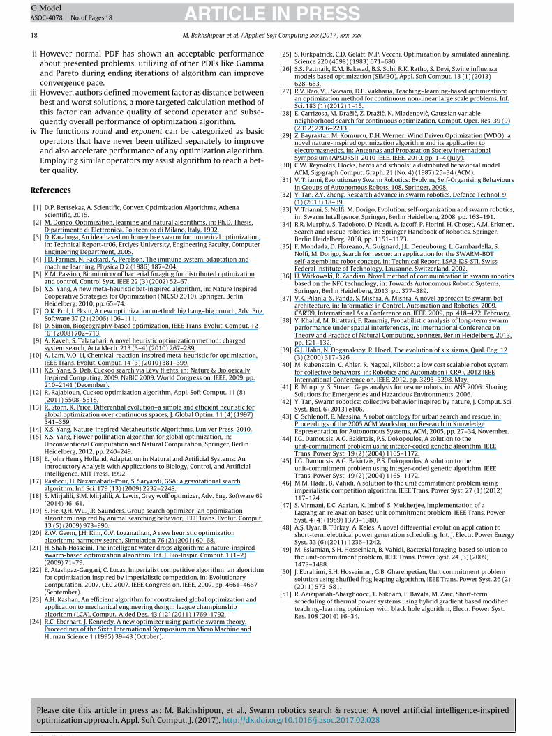
ING Model
Soft C
i
[
[
[
[
[[
[
[
[
[
[
[
[
[
[
[
[
[
[
[
[
[
[
[
[
[
[
[
[
[
[
[
[
[
[
[
[
[
[
[
[
(2011) 573–581.[51] R. Azizipanah-Abarghooee, T. Niknam, F. Bavafa, M. Zare, Short-term
scheduling of thermal power systems using hybrid gradient based modified
ARTICLEASOC-4078; No. of Pages 18
18 M. Bakhshipour et al. / Applied
ii However normal PDF has shown an acceptable performanceabout presented problems, utilizing of other PDFs like Gammaand Pareto during ending iterations of algorithm can improveconvergence pace.
ii However, authors defined movement factor as distance betweenbest and worst solutions, a more targeted calculation method ofthis factor can advance quality of second operator and subse-quently overall performance of optimization algorithm.
iv The functions round and exponent can be categorized as basicoperators that have never been utilized separately to improveand also accelerate performance of any optimization algorithm.Employing similar operators my assist algorithm to reach a bet-ter quality.
References
[1] D.P. Bertsekas, A. Scientific, Convex Optimization Algorithms, AthenaScientific, 2015.
[2] M. Dorigo, Optimization, learning and natural algorithms, in: Ph.D. Thesis,Dipartimento di Elettronica, Politecnico di Milano, Italy, 1992.
[3] D. Karaboga, An idea based on honey bee swarm for numerical optimization,in: Technical Report-tr06, Erciyes University, Engineering Faculty, ComputerEngineering Department, 2005.
[4] J.D. Farmer, N. Packard, A. Perelson, The immune system, adaptation andmachine learning, Physica D 2 (1986) 187–204.
[5] K.M. Passino, Biomimicry of bacterial foraging for distributed optimizationand control, Control Syst. IEEE 22 (3) (2002) 52–67.
[6] X.S. Yang, A new meta-heuristic bat-inspired algorithm, in: Nature InspiredCooperative Strategies for Optimization (NICSO 2010), Springer, BerlinHeidelberg, 2010, pp. 65–74.
[7] O.K. Erol, I. Eksin, A new optimization method: big bang–big crunch, Adv. Eng.Software 37 (2) (2006) 106–111.
[8] D. Simon, Biogeography-based optimization, IEEE Trans. Evolut. Comput. 12(6) (2008) 702–713.
[9] A. Kaveh, S. Talatahari, A novel heuristic optimization method: chargedsystem search, Acta Mech. 213 (3–4) (2010) 267–289.
10] A. Lam, V.O. Li, Chemical-reaction-inspired meta-heuristic for optimization,IEEE Trans. Evolut. Comput. 14 (3) (2010) 381–399.
11] X.S. Yang, S. Deb, Cuckoo search via Lévy flights, in: Nature & BiologicallyInspired Computing, 2009, NaBIC 2009. World Congress on. IEEE, 2009, pp.210–2141 (December).
12] R. Rajabioun, Cuckoo optimization algorithm, Appl. Soft Comput. 11 (8)(2011) 5508–5518.
13] R. Storn, K. Price, Differential evolution–a simple and efficient heuristic forglobal optimization over continuous spaces, J. Global Optim. 11 (4) (1997)341–359.
14] X.S. Yang, Nature-Inspired Metaheuristic Algorithms, Luniver Press, 2010.15] X.S. Yang, Flower pollination algorithm for global optimization, in:
Unconventional Computation and Natural Computation, Springer, BerlinHeidelberg, 2012, pp. 240–249.
16] E. John Henry Holland, Adaptation in Natural and Artificial Systems: AnIntroductory Analysis with Applications to Biology, Control, and ArtificialIntelligence, MIT Press, 1992.
17] Rashedi, H. Nezamabadi-Pour, S. Saryazdi, GSA: a gravitational searchalgorithm, Inf. Sci. 179 (13) (2009) 2232–2248.
18] S. Mirjalili, S.M. Mirjalili, A. Lewis, Grey wolf optimizer, Adv. Eng. Software 69(2014) 46–61.
19] S. He, Q.H. Wu, J.R. Saunders, Group search optimizer: an optimizationalgorithm inspired by animal searching behavior, IEEE Trans. Evolut. Comput.13 (5) (2009) 973–990.
20] Z.W. Geem, J.H. Kim, G.V. Loganathan, A new heuristic optimizationalgorithm: harmony search, Simulation 76 (2) (2001) 60–68.
21] H. Shah-Hosseini, The intelligent water drops algorithm: a nature-inspiredswarm-based optimization algorithm, Int. J. Bio-Inspir. Comput. 1 (1–2)(2009) 71–79.
22] E. Atashpaz-Gargari, C. Lucas, Imperialist competitive algorithm: an algorithmfor optimization inspired by imperialistic competition, in: EvolutionaryComputation, 2007, CEC 2007. IEEE Congress on. IEEE, 2007, pp. 4661–4667(September).
23] A.H. Kashan, An efficient algorithm for constrained global optimization and
Please cite this article in press as: M. Bakhshipour, et al., Swarm rooptimization approach, Appl. Soft Comput. J. (2017), http://dx.doi.org
application to mechanical engineering design: league championshipalgorithm (LCA), Comput.-Aided Des. 43 (12) (2011) 1769–1792.
24] R.C. Eberhart, J. Kennedy, A new optimizer using particle swarm theory,Proceedings of the Sixth International Symposium on Micro Machine andHuman Science 1 (1995) 39–43 (October).
View publication statsView publication stats
PRESSomputing xxx (2017) xxx–xxx
25] S. Kirkpatrick, C.D. Gelatt, M.P. Vecchi, Optimization by simulated annealing,Science 220 (4598) (1983) 671–680.
26] S.S. Pattnaik, K.M. Bakwad, B.S. Sohi, R.K. Ratho, S. Devi, Swine influenzamodels based optimization (SIMBO), Appl. Soft Comput. 13 (1) (2013)628–653.
27] R.V. Rao, V.J. Savsani, D.P. Vakharia, Teaching–learning-based optimization:an optimization method for continuous non-linear large scale problems, Inf.Sci. 183 (1) (2012) 1–15.
28] E. Carrizosa, M. Drazic, Z. Drazic, N. Mladenovic, Gaussian variableneighborhood search for continuous optimization, Comput. Oper. Res. 39 (9)(2012) 2206–2213.
29] Z. Bayraktar, M. Komurcu, D.H. Werner, Wind Driven Optimization (WDO): anovel nature-inspired optimization algorithm and its application toelectromagnetics, in: Antennas and Propagation Society InternationalSymposium (APSURSI), 2010 IEEE. IEEE, 2010, pp. 1–4 (July).
30] C.W. Reynolds, Flocks, herds and schools: a distributed behavioral modelACM, Sig-graph Comput. Graph. 21 (No. 4) (1987) 25–34 (ACM).
31] V. Trianni, Evolutionary Swarm Robotics: Evolving Self-Organising Behavioursin Groups of Autonomous Robots, 108, Springer, 2008.
32] Y. Tan, Z.Y. Zheng, Research advance in swarm robotics, Defence Technol. 9(1) (2013) 18–39.
33] V. Trianni, S. Nolfi, M. Dorigo, Evolution, self-organization and swarm robotics,in: Swarm Intelligence, Springer, Berlin Heidelberg, 2008, pp. 163–191.
34] R.R. Murphy, S. Tadokoro, D. Nardi, A. Jacoff, P. Fiorini, H. Choset, A.M. Erkmen,Search and rescue robotics, in: Springer Handbook of Robotics, Springer,Berlin Heidelberg, 2008, pp. 1151–1173.
35] F. Mondada, D. Floreano, A. Guignard, J.L. Deneubourg, L. Gambardella, S.Nolfi, M. Dorigo, Search for rescue: an application for the SWARM-BOTself-assembling robot concept, in: Technical Report, LSA2-I2S-STI, SwissFederal Institute of Technology, Lausanne, Switzerland, 2002.
36] U. Witkowski, R. Zandian, Novel method of communication in swarm roboticsbased on the NFC technology, in: Towards Autonomous Robotic Systems,Springer, Berlin Heidelberg, 2013, pp. 377–389.
37] V.K. Pilania, S. Panda, S. Mishra, A. Mishra, A novel approach to swarm botarchitecture, in: Informatics in Control, Automation and Robotics, 2009.CAR’09, International Asia Conference on. IEEE, 2009, pp. 418–422, February.
38] Y. Khaluf, M. Birattari, F. Rammig, Probabilistic analysis of long-term swarmperformance under spatial interferences, in: International Conference onTheory and Practice of Natural Computing, Springer, Berlin Heidelberg, 2013,pp. 121–132.
39] G.J. Hahn, N. Doganaksoy, R. Hoerl, The evolution of six sigma, Qual. Eng. 12(3) (2000) 317–326.
40] M. Rubenstein, C. Ahler, R. Nagpal, Kilobot: a low cost scalable robot systemfor collective behaviors, in: Robotics and Automation (ICRA), 2012 IEEEInternational Conference on. IEEE, 2012, pp. 3293–3298, May.
41] R. Murphy, S. Stover, Gaps analysis for rescue robots, in: ANS 2006: SharingSolutions for Emergencies and Hazardous Environments, 2006.
42] Y. Tan, Swarm robotics: collective behavior inspired by nature, J. Comput. Sci.Syst. Biol. 6 (2013) e106.
43] C. Schlenoff, E. Messina, A robot ontology for urban search and rescue, in:Proceedings of the 2005 ACM Workshop on Research in KnowledgeRepresentation for Autonomous Systems, ACM, 2005, pp. 27–34, November.
44] I.G. Damousis, A.G. Bakirtzis, P.S. Dokopoulos, A solution to theunit-commitment problem using integer-coded genetic algorithm, IEEETrans. Power Syst. 19 (2) (2004) 1165–1172.
45] I.G. Damousis, A.G. Bakirtzis, P.S. Dokopoulos, A solution to theunit-commitment problem using integer-coded genetic algorithm, IEEETrans. Power Syst. 19 (2) (2004) 1165–1172.
46] M.M. Hadji, B. Vahidi, A solution to the unit commitment problem usingimperialistic competition algorithm, IEEE Trans. Power Syst. 27 (1) (2012)117–124.
47] S. Virmani, E.C. Adrian, K. Imhof, S. Mukherjee, Implementation of aLagrangian relaxation based unit commitment problem, IEEE Trans. PowerSyst. 4 (4) (1989) 1373–1380.
48] A.S. Uyar, B. Türkay, A. Keles, A novel differential evolution application toshort-term electrical power generation scheduling, Int. J. Electr. Power EnergySyst. 33 (6) (2011) 1236–1242.
49] M. Eslamian, S.H. Hosseinian, B. Vahidi, Bacterial foraging-based solution tothe unit-commitment problem, IEEE Trans. Power Syst. 24 (3) (2009)1478–1488.
50] J. Ebrahimi, S.H. Hosseinian, G.B. Gharehpetian, Unit commitment problemsolution using shuffled frog leaping algorithm, IEEE Trans. Power Syst. 26 (2)
botics search & rescue: A novel artificial intelligence-inspired/10.1016/j.asoc.2017.02.028
teaching–learning optimizer with black hole algorithm, Electr. Power Syst.Res. 108 (2014) 16–34.