sustainable optimal strategic planning for shale water...

Sustainable Optimal Strategic Planning for Shale Water

Management

Alba Carrero-Parreñoa, Juan A. Reyes-Labarta*a,b, Raquel Salcedo-Díaza,b, Rubén Ruiz-

Femeniaa,b, José A. Caballeroa,b, Ignacio E. Grossmannc

aInstitute of Chemical Process Engineering, University of Alicante, Ap Correos 99,

Alicante 03080, Spain bDepartment of Chemical Engineering, University of Alicante, Ap Correos 99, Alicante

03080, Spain cDepartment of Chemical Engineering, Carnegie Mellon University, Pittsburgh, PA

15213, U.S.A.

* Corresponding author at. Institute of Chemical Process Engineering, University of

Alicante, Ap Correos 99, Alicante 03080, Spain. Phone: +34 965903867. [email protected]

ABSTRACT

In this work, we introduce a non-convex MINLP optimization model for water

management in shale gas production. The superstructure includes direct reuse in the same

or neighboring wellpads, treatment in mobile units and in centralized water treatment

(CWT) facility, and transport to Class II disposal wells. We consider four different water

qualities: flowback water, impaired water, desalinated water and freshwater.

Additionally, water blending ratios are unrestricted and friction reducers expenses are

calculated accounting for impaired water contamination. The objective is to optimize the

fracturing schedule, the number of tanks needed at each time period, flowback destination

(reuse, treated or disposal), and fracturing fluid composition by maximizing the

“sustainability profit”. The problem is tackled in two steps. First, we solve an MILP

model based on McCormick relaxations. Second, a smaller MINLP is solved in which the

binary variables that determine the fracturing schedule are fixed. The capabilities of the

proposed mathematical model are validated against several case studies based on

Marcellus Shale play.

mailto:[email protected]

A. Carrero-Parreño et al.

2

INTRODUCTION

Natural gas production worldwide is expected to increase 62% by 2040. The largest

component in the projected growth is due to shale gas production, which will increase

from 342 billion cubic feet per day (Bcf/d) in 2015 to 554 Bcf/d by 2040.1 Currently, only

United States, Canada, China and Argentina have commercial shale gas production.

However, Mexico and Algeria are expected to contribute to the projected growth due to

the technological improvements made in the extraction techniques.1,2

It is well-known that the extraction of shale gas, apart from generating huge benefits, has

associated environmental risks including many water-based concerns. The exploitation of

a shale gas well includes exploration, wellpad construction, well drilling, well treatment

and completion, and production. The largest volume of water used is during well

treatment and completion where hydraulic fracturing occurs. Operators fracture shale gas

wells in 8 to 23 stages, using from 190 to 38,000 m3 of fracturing fluid per well depending

on shale gas formation.3 Fracturing fluids typically contain about 90% water, 9%

propping agent and less than 1% of friction‐reducing additives.3,4 After the well is

hydraulically fractured, the pressure of the wellhead is released allowing a portion of

wastewater, called flowback water, return to the wellhead. Flowback is recovered from

few days to few weeks containing total dissolved solids (TDS) ranging from 10,000 to

150,000 mg L-1. The wastewater that continues generating over the life of the well (10 -

30 years) is called produce water. The TDS concentration in long-term produce water can

reach 250,000 mg L-1. Both wastewater volume and concentration of TDS is uncertain

and varies with the geographical properties of the formation. As a rule of thumb, the

volume of wastewater generated is 50 percent flowback water and 50 percent produce

water.3


3

Current water management strategies include disposal of wastewater via Class II disposal

wells, transfer to a centralized water treatment facility (CWT) or direct reuse in drilling

the subsequent wells. The reused flowback is called impaired water. This water

management strategy has been possible due to the development of salt-tolerant friction

reducers.3,5,6 Previous friction reducers were not compatible with salt-water, therefore

they were not able to control friction pressure losses and associated pump pressure. Direct

reuse in drilling the subsequent wells is currently the most popular option due to its

operational simplicity for contractors.7 Moreover, this practice has the potential to

decrease the environmental issues associated with shale gas water management such as

transportation, disposal or treatment. However, the cost of friction reducers increases

with the concentration of TDS. Operators must take into consideration that reusing

impaired water, the concentration of TDS will increase over the time representing a major

cost-barrier.

Several works have been reported on the optimization of shale gas water management.

Yang et. al8 proposed a discrete-time two-stage stochastic mixed-integer linear

programming model to determine - in short-term operations - the optimal fracturing

schedule and transportation, storage, treatment and disposal cost under uncertain

availability water. The model does not account for TDS concentration. They developed

an extended model 9 accounting for TDS to consider long-term decisions for investments

in water treatment, impoundments and pipelines. However, to avoid non linearities they

used an approximation by discretizing the TDS concentration. Bartholomew and Mauter10

used the Yang et. al model9 integrating human health and environmental impacts with

multi-objective optimization. However, the authors do not consider return to pad

operations, and fixed the blending ratio a priori. Gao and You11 proposed a mixed-integer

linear fractional programming model to maximize the profit per unit of freshwater


4

consumption. The authors include multiple transportation modes and water management

options. Nevertheless, they also do not consider return to pad operations and they fixed

the blending ratio and fracturing schedule a priori. Gao and You12 also presented a mixed-

integer nonlinear programming problem addressing the life-cycle economic and

environmental optimization of shale gas supply chain network. Guerra et al.13 presented

an optimization framework that integrates water management and the design and planning

of the shale gas supply chain. In this case, the fracturing schedule and sizing of storage

facilities are out of the scope of the proposed framework. Moreover, they do not consider

reusing water directly, without treatment. Lira-Barragán et. al14 presented a mathematical

model for synthesizing shale gas water networks accounting uncertainty in water demand

for hydraulic fracturing and flowback water forecast. Lira-Barragán et. al15 also

developed an MILP mathematical programming formulation accounting for economics

by minimizing the cost for the freshwater, treatment, storage, disposals, and

transportation, and minimizing freshwater usage and wastewater discharge as an

environmental objectives. However, in both works the schedule is fixed in advance, and

the wastewater is always treated. Recently, Drouven and Grossmann16 proposed an MILP

model to identify the optimal strategies for impaired water overestimating the cost of

friction reducers. The authors consider return to pad operations and assume that the water-

blending ratio is unrestricted. However, the mathematical model does not account for

other water management strategies nor the salt concentration of impaired water.

This paper focuses on overcoming some of the limitations of the previous papers cited

above. Specifically, we propose a mixed-integer non-linear programming (MINLP)

model that considers the TDS concentration of flowback and impaired water, as well as

different water treatment solutions. The main novelties introduced in this work comprise:

(a) estimation of friction reducers expenses as a function of TDS concentration to


5

determine if the level of TDS in impaired water is an impediment for reusing it in

fracturing operations; (b) distinction of four types of water: impaired water, flowback

water, desalinated water and freshwater; and (c) rigorous handling at storage solution by

determining the required number of tanks installed/uninstalled over the time period.

The objective of the proposed model is to maximize the “sustainability profit”17 in order

to obtain a compromise solution between economic, environmental and social aspects.

The advantage of this metric is that multi-objective optimization can be reduced to a

single-objective since all the indicators are expressed in monetary terms.

The rest of the paper is organized as follows: Section 2 describes the problem statement.

In section 3, the mathematical MINLP model is described in detail. In section 4, the

modeling and solution strategy are described. The results obtained from different case

studies based on Marcellus play are presented in section 5. Finally, the last section

summarizes the conclusions of the present work.

PROBLEM STATEMENT

The problem studied in this paper can be stated as follows. Given are the following:

• A set of shale gas wells belonging a specific wellpads including water requirements,

fracturing time and crews available to perform the drilling and completion phase.

Profiles for the flowback flowrate, TDS concentration and gas production curve per

well are also provided.

• The capacity and the maximum number of fracturing tanks. Each storage unit

includes the cost associated to move, demobilize and clean out the tank before

removing it from the location and leasing cost.

• The capacity and the maximum number of freshwater tanks available to store the

water required to complete each well.


6

• The capacity and the maximum number of impoundments. Freshwater can also be

stored in freshwater impoundments.

• A set of freshwater sources available to supply the water for hydraulic fracturing

operations and the water withdrawal cost.

• A set of Class II disposal wells to inject the wastewater and the corresponding cost

of disposal.

• A set of treatment technologies to desalinate the flowback water onsite. The

maximum capacity, treatment cost, leasing cost and the cost associated to move,

demobilize and clean out are also given.

• A set of centralized water treatment (CWT) plants and the treatment cost and

maximum capacity of each facility.

• Locations of freshwater source, centralized water treatment (CWT), disposal wells

and wellpads.

• Transportation costs of freshwater and wastewater via trucks.

• The cost of moving rigs, well drilling and completion, shale gas production and

friction reducers are given.

• The sales price of shale gas per week for all prospective wells is provided.

The problem is to determine: wellpad fracturing start date (fracturing schedule), number

of tanks leased at each time period, flowback destination (reuse, treatment or disposal),

and type and location of onsite desalination treatment at each time period.

The superstructure proposed for water management in shale gas operations is shown in

Figure 1.


7

Figure 1. General superstructure of shale gas water management operations.

The water management system comprises wellpads p, shale gas wells in each wellpad w,

centralized water treatment technologies (CWT) k, natural freshwater sources f, fracturing

crew c, and disposal wells d.

As commented before, after hydraulic fracturing, a portion of the water called flowback

water returns to the wellhead. The flowback water is stored onsite in fracturing tanks (FT)

before basic treatment (pre-treatment) in mobile units, or else transported to CWT facility,

Class II disposal, or to a neighboring wellpad. Pre-treatment includes technologies to

remove suspended solids, oil and grease, bacteria and certain ions that can cause the scale

to form on equipment and interfere with fracturing chemical additives.18 After pre-

treatment, the water can be used directly as a fracturing fluid in the same or neighboring

wellpad, or it can be desalinated in the onsite TDS removal technologies.

Two desalination technologies can be selected such as multi-stage membrane distillation

(MSMD)19 and multi-effect evaporation with mechanical vapor recompression (MEE-

MVR)20,21. We consider that the outflow brine salinity in the onsite treatment is close to

External water

source f

W1 W2

(…)WIWI

Disposal well d

OT

f1

f2

fIFI

d1

d2

dIDI

CWT plant k

Well pad p

k1 k2

kIKI

From wellpad p

from wellpad p

Discharge

Discharge

Fracturing fluidDesalinated water

Freshwaterflowback

water

Impairedwater

FWT: Freshwater tank / FT: Fracturing tank /OP: Onsite pre-treatment /OT: Onsite treatment

to wellpad p

to wellpad p

FTFWT

OP

BrineBrine


8

salt saturation conditions to achieve zero liquid discharge (ZLD) operation, maximizing

at the same time the recovered freshwater. Costs restrict the type of desalination unit that

can be used for TDS removal. The onsite desalinated water can also be used as a fracturing

fluid in the same wellpad, transported to the next wellpad, or discharged for other uses.

The flowback water can also be transported and treated in CWT plants. Desalinated water

from CWT plants can select the same routes as the desalinated water in onsite

technologies. Natural freshwater is obtained from an uninterruptible freshwater source.

Desalinated water and natural freshwater are stored in freshwater tanks (FWT) and/or

water impoundment.

The assumptions made in this work are as follows:

• A fixed time horizon is discretized into weeks as time intervals.

• The volume of water required to fracture each well is available at the beginning of

well development, and includes the water used in drilling, construction and

completion.

• Onsite pretreatment (OP) process provides adequate contaminant removal for the

next operations.

• Friction reducers costs increase linearly with the concentration of salts.

• Transportation is only performed by trucks.

MATHEMATICAL PROGRAMMING MODEL

The optimization problem is formulated as an MINLP model that includes: assignment

constraints, material balance in storage tanks, mixers and splitters, logic constraints, and

an objective function. The mathematical problem is detailed below.

Set definition

The following sets are defined to develop the MINLP model.


9

/ is a wellpad

/ is a well

/ is a time period

/ is a onsite water treatment

/ is centralized water treatment plant

/ is a freshwater source

/ is a fracturing crew

/ is a dispo

P p p

W w w

T t t

N n n

K k k

F f f

C c c

D d d

=

=

=

=

=

=

=

=

sal

/ is a storage tank type

/ is a well in wellpad pp

S s s

RPW w w

=

=

Assignment constraint

Eq. (1) ensures that at the time horizon each well can be fractured by one of the available

fracturing crew c,

, , , 1 ,hft p w c p

t T c C

y w RPW p P

(1)

where 𝑦𝑡,𝑝,𝑤,𝑐ℎ𝑓

indicates that the well w in wellpad p is stimulating by fracturing crew c in

time period t.

Eq. (2) guarantees that there is no overlap in the hydraulic fracturing operations between

different wells,

, , ,

1

1 ,

p w

thftt p w c

p P w RPW tt t

y t T c C = − +

(2)

where 𝜏𝑤 is a parameter that indicates the time required to fracture well w by fracturing

crew c.

Shale water composition and water recovered

After a well is hydraulically fractured, a portion of the water injected is returned to the

wellhead,

, , , , ,, ,

w

hf fbt p w c w pt p w

c C

y y t T w RPW p P

+

= − (3)


10

where 𝑦𝑡,𝑝,𝑤,𝑐𝑓𝑏

represents the time period when the flowback water comes out. The binary

variable 𝑦𝑡,𝑝,𝑤,𝑐𝑓𝑏

is treated as a continuous variable since its integrality is enforced by

constraint (3).

The shale gas water recovered and composition from each wellpad, once the well is

hydraulically fractured, is calculated with Eqs. (4-5),

1

, , , , 1, ,0

, ,tt t

well well fbt p w t tt p w ptt p w

tt

f F y t T w RPW p P −

− +=

= (4)

1

, , , , 1, ,0

, ,tt t

well well fbt p w t tt p w ptt p w

tt

c C y t T w RPW p P −

− +=

= (5)

where, 𝐹𝑡,𝑝,𝑤𝑤𝑒𝑙𝑙 and 𝐶𝑡,𝑝,𝑤

𝑤𝑒𝑙𝑙 are parameters that indicate flowback flowrate and TDS

concentration at week, respectively.

Eqs. (6-7) correspond to the mass and salt balance of flowback water collected from the

wells belonging the wellpad p,

, , , ,

p

pad wellt p t p w

w RPW

f f t T p P

= (6)

, , , , , , ,

p

pad pad well wellt p t p t p w t p w

w RPW

c f C F t T p P

= (7)

Mass and salt balance in storage tanks

The level of the storage tank in each time period (𝑠𝑡𝑡,𝑝,𝑠) depends on the water stored in

the previous time period (𝑠𝑡𝑡−1,𝑝,𝑠), the mass flowrates of the inlet streams belonging the

storage tank s, and the mass flowrates of the outlet streams belonging the storage tank s.

1, , , , , , , , , ,i ot p s t p s t p s t p s

i IS o OS

st f st f t T p P s S−

+ = + (8)

The salt mass balance in fracturing tank is described by the following equation,


11

1, , 1, , , , , , , , ,

, ,

i i ot p s t p t p s t p t p s t p s t p

i IS o OS

st c f c st f c

t T p P s ft

− −

+ = +

(9)

Storage balances

Flowback water and freshwater are stored in portable leased tanks at wellpad p. Eq. (10)

describes the storage balance of tank s in wellpad p in time period t,

, , 1, , , , , , , ,ins uninst p s t p s t p s t p sn n n n t T p P s S−= + −

(10)

where 𝑛𝑡,𝑝,𝑠 is the total number of tanks, 𝑛𝑡,𝑝,𝑠𝑖𝑛𝑠 and 𝑛𝑡,𝑝,𝑠

𝑢𝑛𝑖𝑛𝑠 represent the number of

installed or uninstalled tanks in a specific time period.

The amount of water stored 𝑠𝑡𝑡,𝑝,𝑠 is bounded by the capacity of one tank 𝐶𝑆𝑇𝑠 and the

number of tanks installed. As the time horizon is discretized into weeks, the storage tank

should handle the inlet water that comes from one day. Therefore, 𝜃𝑡,𝑝,𝑠 represents the

inlet water in the storage tank divided by the number of days in a week to avoid oversizing

the tanks,

, , , , , , , ,t p s t p s s t p sst CST n t T p P s ft+ (11)

, , , , , , , ,LO st ins UP sts t p s t p s s t p sN y n N y t T p P s S (12)

𝑁𝑠𝐿𝑂 and 𝑁𝑠

𝑈𝑃 are lower and upper bounds of the number of tanks installed. 𝑦𝑡,𝑝,𝑠 𝑠𝑡 indicates

the installation of each tank s on wellpad p at time period t.

The total freshwater stored also depends on the number of freshwater impoundments

installed,

,, 1, , ,im im im ins

t p t p t pn n n t T p P−= + (13)

, , ,, , , ,im LO im im ins im UP im

t p t p t pN y n N y t T p P (14)


12

, , , , , , , , ,imp imt p s t p s s t p s t pst CST n V n t T p P s fwt+ + (15)

where impV is the capacity of an impoundment.

Water Demand

The amount of water required per wellpad (𝑓𝑡,𝑝𝑑𝑒𝑚) can be supplied by a mixture of fresh

(𝑓𝑡,𝑝𝑓𝑟𝑒𝑠ℎ

) or impaired water (𝑓𝑡,𝑝𝑖𝑚𝑝

),

, , , ,dem fresh impt p t p t pf f f t T p P= + (16)

The fracturing water (𝑓𝑡,𝑝,𝑤𝑑𝑒𝑚) required in each well is given by constraint (17),

, , , ,

p

dem demt p t p w

w RPW

f f t T p P

= (17)

The following constraint indicates that the water available at each well, when the well is

fractured must be greater or equal than the water demand of each well (𝑊𝐷𝑤),

, , , , , , ,dem hft p w w t p w c p

c C

f WD y t T w RPW p P

(18)

Onsite treatment

Mass balance around onsite pretreatment technology is described in Eq.(19),

, , ,, , , ,pre out on slud pre in

t p t p t pf f f t T p P+ = (19)

The relation between inlet and outlet mass flowrate is modeled by using the recovery

factor (𝛼𝑝𝑟𝑒),

, ,, , ,pre out pre pre in

t p t pf f t T p P= (20)

After pretreatment, the water can be used as a fracturing fluid (𝑓𝑡,𝑝𝑖𝑚𝑝

) or/and can be sent

to desalination technology (𝑓𝑡,𝑝𝑜𝑛,𝑖𝑛

),

, ,, , , ,pre out imp on in

t p t p t pf f f t T p P= + (21)


13

The total and salt balances around the onsite desalination treatment are given by Eqs. (22-

23). In order to achieve the outlet stream close to ZLD conditions, the outlet brine salinity

(𝐶𝑧𝑙𝑑) is fixed to 300 g·kg-1 (close to salt saturation condition of ̴ 350 g·kg-1).

, , ,, , , ,on out on brine on in

t p t p t pf f f t T p P+ = (22)

, ,, , , ,on brine zld on in

t p t p t pf C f c t T p P = (23)

Two options have been considered for TDS reduction such as MSMD and MEE-MVR.

The onsite desalination treatment is also leased. Hence, onsite treatment balance is

described in the following equations.

, ,, , 1, , , , , , , ,on on on ins on unins

t p n t p n t p n t p nn n n n t T p P n N−= + − (24)

The number of onsite treatment leased depends on the total number of portable treatments

available.

, , ,, , , , , , , ,on LO on on ins on UP on

n t p n t p n n t p nN y n N y t T p P n N (25)

Eq (26) represents the mass balance through the desalination unit,

, ,, , , ,on in on in

t p t p n

n N

f f t T p P

= (26)

The following equation Eq. (27) represents the selection of treatment units and their

maximum capacity.

, , ,, , , , , , , ,on LO on on in on UP on

n t p n t p n n t p nF y f F y t T p P n N (27)

The flow directions for the desalinated water are given by Eq.(28). 𝑓𝑡,𝑝𝑜𝑛,𝑓𝑤𝑡

is the

desalinated water sent to freshwater tank, 𝑓𝑡,𝑝𝑜𝑛,𝑑𝑒𝑠 is the water discharged on the surface

and 𝑓𝑡,𝑝,𝑝𝑝𝑝𝑎𝑑,𝑓𝑤𝑡

is the desalinated water used as a fracturing fluid in the same or other

wellpad,


14

, , , ,, , , , , ,on out on fwt on des pad fwt

t p t p t p t p pp

pp P

f f f f t T p P

= + + (28)

Centralized water treatment

In this section, mass balances are performed in the CWT facility. Eq. (29) shows the

relationship between inlet and outlet streams, and Eq. (30) constraints the inlet flowrate

of CWT k with the maximum flowrate allowed.

, ,, , , ,cwt out rec cwt in

t k k t p k

p P

f f t T k K

= (29)

, ,, , ,cwt in cwt UP

t p k k

p P

f F t T k K

(30)

The freshwater mass balance at the end of CWT k is given by Eq.(31),

, , ,, ,, , ,cwt out cwt fwt cwt des

t k t kt p kp P

f f f t T k K

= + (31)

Sustainability profit – Objective function

The objective function to be maximized includes the economic profit (PEconomic), eco-cost

(CEco) and social profit (PSocial).

Economic Eco Socialmax SP P C P= − + (32)

Economic profit includes revenues from natural gas minus the sum of the following

expenses: drilling and production cost, wastewater disposal cost, storage tank cost,

freshwater cost, friction reducer cost, wastewater and freshwater transport cost and onsite

and offsite treatment cost.

( )Economic gas drill dis sto source fr trans ondes cwt crewP R E E E E E E E E E= − + + + + + + + + (33)

The revenues of shale gas sales can be represented by Eq. (34),

1

, , 1, ,0p

tt tgas gas fb gas

t tt p w ttt p wt T p P w RPW tt

R F y −

− + =

= (34)


15

where 𝐹𝑡,𝑝,𝑤𝑔𝑎𝑠

is the gas production and 𝛼𝑡𝑔𝑎𝑠

is the gas price forecast in time period t.

Drilling, completion and production cost are defined by Eq. (35),

, , , , ,

p p

drill drill hf prod gast p w c t p w

t T p P w RPW c C t T p P w RPW

E y f

= + (35)

Disposal expenses only include the disposal costs 𝛼𝑑𝑑𝑖𝑠 which depend on the place where

the class II disposal well is located,

, ,dis dis dis

d t p d

t T p P d D

E f

= (36)

Fracturing, impaired water and freshwater tanks are typically leased, the cost is made up

of leasing cost (𝛼𝑠𝑠𝑡𝑜) and mobilize, demobilize and cleaning cost (𝛽𝑠

𝑠𝑡𝑜) as follows,

( ) ,, , , , ,

sto sto sto ins im im ins ims t p s s t p s t p

t T p P s S t T p P

E n n n V

= + + (37)

Where 𝛼𝑖𝑚 represents the cost of the impoundments construction. The freshwater cost

includes the withdrawal cost from the diverse sources f,

, ,source source source

f t p f

t T p P f F

E f

= (38)

The friction reducers costs are given by Eq.(39). They depend on the TDS concentration

and the flowrate used for hydraulic fracturing,

( ), ,fr fr fr imp

t p t p

t T p P

E c f

= + (39)

Transportation expenses by truck involve the sum of the following transfers: (1) from

wellpad p to disposal location d, (2) from freshwater source f to wellpad p, (3) from

wellpad p to offsite treatment k, and (4) from wellpad p to wellpad pp.

( )

( )

, , , ,, ,

, ,, , , ,

,, , , , ,

+

+

+

dis pad dis source pad sourcet p d t p fp d f p

d D f F

truck truck cwt in cwt fwt pad cwtt k t p k p k

t T p P k K

pad pad imp pad padt p pp t p pp p pp

pp P

f D f D

E f f D

f f D

− −

−

−

= +

+

(40)


16

where 𝐷𝑝,𝑑𝑝𝑎𝑑−𝑑𝑖𝑠

, 𝐷𝑝,𝑓𝑝𝑎𝑑−𝑠𝑜𝑢𝑟𝑐𝑒

, 𝐷𝑝,𝑘𝑝𝑎𝑑−𝑐𝑤𝑡

and 𝐷𝑝,𝑝𝑝𝑝𝑎𝑑−𝑝𝑎𝑑

are the distances from wellpad p

to disposal site d, source f, CWT facility and wellpad pp.

Pretreatment expenses depend on the wastewater destination. Obviously, requirements to

desalinate the water in thermal treatment or membrane treatments are more restrictive

than the requirements to reuse it in fracturing operations. As described in Eq. (41), 𝛼𝑟𝑒𝑢𝑠𝑒

represents the pretreatment cost aiming its reuse, and 𝛼𝑡𝑟𝑒𝑎𝑡 the pretreatment cost aiming

to remove TDS by desalination technologies. Onsite TDS removal unit cost includes

desalination cost (𝛼𝑛𝑜𝑛), mobilize, desmobilize and cleaning cost (𝛽𝑛

𝑜𝑛) and leasing cost

(𝛼𝑛𝑜𝑛 ).

, ,, , , , , ,[ ( )]ondes reuse imp treat on in on on on on inst

t p t p n t p n n t p n

t T p P n N

E f f n n

= + + + (41)

The CWT cost is given by Eq. (42) and it depends on the cost that the treatment plant

imposes for treating the flowback water from shale gas operations (𝛼𝑘𝑐𝑤𝑡).

,, ,

cwt cwt cwt ink t p k

t T p P k K

E f

= (42)

The cost of moving crews and rigs depends if the candidate well is going to be fractured

in the same or other wellpad. With that purpose, the binary variable 𝑦𝑡,𝑝,𝑐𝑐𝑟𝑒𝑤 is equal to 1 if

at least one well is drilled in wellpad p in time period t by crew c,

, , , , , , ,

p

crew frt p c t p w c

w RPW

y y t T p P c C

(43)

, , 1 ,crewt p c

p P

y t T c C

(44)

, , 1, ,( )crew crew crew crewt p c t p c

t T p P c C

E y y −

= − (45)

Eco-cost is a robust indicator from cradle-to-cradle LCA calculations in the circular

economy that includes eco-costs of human health, ecosystems, resource depletion and

global warming. The terms are calculated by using eco-cost coefficients.22 In our problem,


17

the eco-cost term includes natural gas extraction, freshwater withdrawal, desalination,

disposal and transportation. The eco-cost to be minimized is defined by Eq. (46),

Eco T Tr r g g r r g g

r R g G r R g G

C q q D q D q

= + + + (46)

where r and g are indices for raw materials and products, respectively. 𝜇 represents eco-

cost of raw materials and products and 𝜇𝑇is the eco-cost of transportation. All coefficients

are proportional to mass flows (𝑞).

Social profit includes social security contributions paid for the employed people to

fracture a well (SS), plus the social transfer by hiring people (SU), minus social cost

(SC).17 We only take into account the number of jobs on a fracturing crew and the time

that they are working to fracture a specific well. Once the well is completed, the number

of jobs generated by truck drivers or maintenance team are not considered. The social-

profit is defined by Eq. (47),

, ,, , , N ( ) N N ( ) hf

w

p

Social

jobs jobs jobs Companyhf Gross Net UNE State EMP Statet p w c

t T p P w RPW c C

P SS SU SC

y S S C C C

= + + =

− + − +

(47)

where 𝑁𝑗𝑜𝑏𝑠 is the number of new jobs needed to fracture a well, 𝑆𝑔𝑟𝑜𝑠𝑠 and 𝑆𝑛𝑒𝑡 are the

average gross and net salaries paid for each employee, 𝐶𝑈𝑁𝐸,𝑆𝑡𝑎𝑡𝑒 is the average social

transfer for unemployed people, 𝐶𝐸𝑀𝑃,𝑆𝑡𝑎𝑡𝑒 is the state social transfer (i.e child allowance,

state scholarship, health insurance) and 𝐶𝑐𝑜𝑚𝑝𝑎𝑛𝑦 is company’s social charge (i.e team

building events, excursions, cultural activities).

SOLUTION STRATEGY

The optimization problem is modeled using total flows and salt composition as variables.

This proposed MINLP model - Eqs. (1)-(47) - involves bilinear terms in the salt water

mass balances - Eqs. (7), (9), (23) and (39). These terms are the source of the non-


18

convexity in the model. An advantage of using this representation is that the bounds of

the variables present in the non-convex bilinear terms can be easily determined. If local

solvers are selected to solve the MINLP problem, we may converge to a local solution.

Global optimization solvers can in principle be used but may not reach a solution for a

large scale non-convex MINLP problems in a reasonable period of time. Thus, we

propose the following decomposition strategy in order to achieve a trade-off between the

solution quality vs time.

• The original MINLP is relaxed using under and over estimators of the bilinear

terms, McCormick convex envelope23, which leads to an MILP. To this aim, the

bilinear terms in constraints (7), (9), (23) and (39) are replaced by the following

equations. The solution of this MINLP yields an upper bound (UB) to the original

MINLP.

LO LO LO LO

UP UP UP UP

UP LO LO UP

UP LO UP LO

s c F C f C FUnderestimators

s C f c F C F

s c F C f C FOverstimators

s C f c F C F

+ −

+ −

+ −

+ −

(48)

where s is the corresponding bilinear term and flow and 𝐶𝐿𝑂, 𝐹𝐿𝑂 , 𝐶𝑈𝑃 and 𝐹𝑈𝑃 are

the lower and upper bound of salt concentrations and flows

• The binary variables obtained in the previous MILP, that determine the fracture

schedule (𝑦𝑡,𝑝,𝑤,𝑐ℎ𝑓

), are fixed into the original MINLP, resulting in a smaller

MINLP involving the binary variables 𝑦𝑡,𝑝,𝑠𝑠𝑡 and 𝑦𝑡,𝑝,𝑛

𝑜𝑛 .

The model is implemented in GAMS 25.0.1.24 The relaxed MILP problem is solved with

Gurobi 7.5.2 25 and the MINLP problem with DICOPT 2 26 using CONOPT 4 27 to solve

the NLP sub-problems. Although DICOPT cannot guarantee a global solution, we


19

calculate the optimality gap defined by Eq. (49) to obtain the deviation of this solution

with respect to the global optimum,

UB LBgap

UB

−= (49)

CASE STUDIES

The case studies shown in Table 1 based on Marcellus Play illustrate the capabilities of

the proposed optimization model. They are composed by 20 wells grouped in 3 wellpads,

one year discretized at one week per time period, three Class II disposal wells, four

interruptible sources of freshwater, two CWT plants and one fracturing crew. The

difference between interruptible sources, disposal wells and CWT plants lies in the

geographical location. Data of the problem – cost coefficients and model parameters -

are given in Appendix A (Table A.1 – A.4). Gross and net salaries paid for each employee

are obtained from the Bureau of Labor Statistics. 28 Our goal is to determine the optimal

water management during the flowback water process. Therefore, we consider the natural

gas production and wastewater generated in the first twelve weeks. Flowback water

generation is the critical period for shale gas water management. In this phase, the

coordination between different contractors is crucial since the water is recovered in a

short time period. The inlet TDS concentration increase with time ranging from 3,000 to

200,000 ppm. We assume that 50% of the water used to fracture a well, which ranges

from 4,800 to 18,600 m3, is recovered as flowback water.

The relaxed MILP problem has 3,273 binary variables, 21,373 continuous variables and

20,600 constraints. In the reduced non-convex MINLP, the binary variables decrease to

2,337 by using the solution of the relaxed MILP problem that provides the fracturing

schedule for the non-convex MINLP. The reduced non-convex MINLP has 14,607


20

continuous variables and 9,361 constraints. The model has been solved on a computer

with a 3 GHz Intel Core Dual Processor and 4 GB RAM running Windows 10.

Table 1. Case study description

Case study Description

Case 1 All water management options are allowed: reuse the flowback water

with a little treatment, desalinate the water in onsite treatment or CWT,

reuse the desalinated water as a fracturing fluid and disposal in class II

disposal wells.

Case 2 Disposal in class II disposal wells is the only water management option

allowed.

Case 3 Wastewater can be sent to onsite desalination treatment or CWT.

Case 4 The cost of friction reducers is overestimated. Eq. (50) is replaced by

the following equation:

,fr fr imp

t p

t T p P

E f

= (50)

Case 5 All water management options, as in Case 1, are allowed. However,

return to pad-operations is not allowed and wells are fractured in order;

well 2 cannot be fractured before well 1. To do this, the following

constraint is added:

, , , , , , , ,hf hft p w c t p ww c p

t T t T

t y t y w ww w RPW p P

(51)

The optimal fracturing schedule for each case study is shown in Figure 2. All wells are

fractured before time period forty. This allows to treat the flowback water and extract the

natural gas that comes from all wells in the first twelve weeks.


21

Figure 2. Fracturing schedule for all case studies.

The fractured schedule for Cases 2, 3 & 4 is the same since the model maximizes the

revenue. A different schedule with lower revenue would reduce the cost to compensate

the change in the revenue. This happens in Case 1, the maximization of the water reuse

to fracture other wells compensate to obtain another fracture schedule with lower revenue

but lower cost.

In all cases, the optimal solution shows that the fracturing schedule includes return to pad-

operations, except in Case 5 where it is prohibited. Therefore, moving the crew from one

wellpad to another without fracturing all wells that belong to the candidate wellpad is

profitable. Return to pad-operations always must take into consideration to the optimal

shale gas fracturing schedule.


22

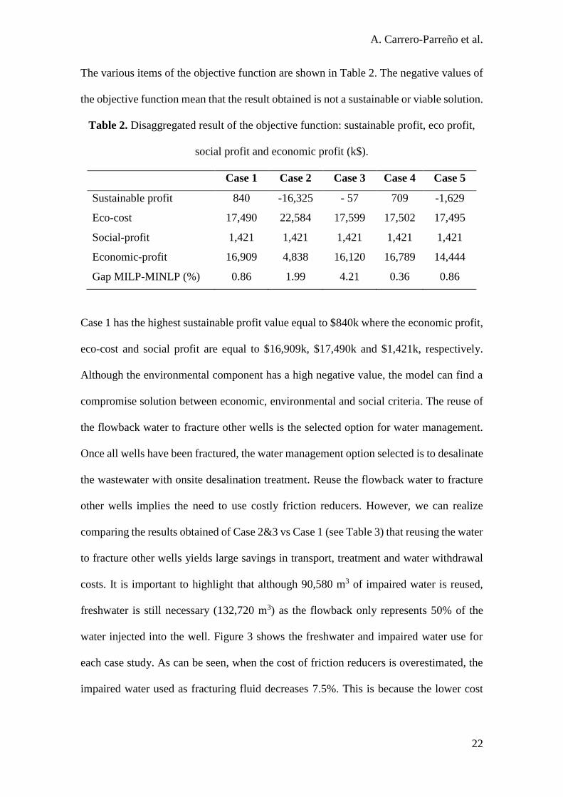
The various items of the objective function are shown in Table 2. The negative values of

the objective function mean that the result obtained is not a sustainable or viable solution.

Table 2. Disaggregated result of the objective function: sustainable profit, eco profit,

social profit and economic profit (k$).

Case 1 Case 2 Case 3 Case 4 Case 5

Sustainable profit 840 -16,325 - 57 709 -1,629

Eco-cost 17,490 22,584 17,599 17,502 17,495

Social-profit 1,421 1,421 1,421 1,421 1,421

Economic-profit 16,909 4,838 16,120 16,789 14,444

Gap MILP-MINLP (%) 0.86 1.99 4.21 0.36 0.86

Case 1 has the highest sustainable profit value equal to $840k where the economic profit,

eco-cost and social profit are equal to $16,909k, $17,490k and $1,421k, respectively.

Although the environmental component has a high negative value, the model can find a

compromise solution between economic, environmental and social criteria. The reuse of

the flowback water to fracture other wells is the selected option for water management.

Once all wells have been fractured, the water management option selected is to desalinate

the wastewater with onsite desalination treatment. Reuse the flowback water to fracture

other wells implies the need to use costly friction reducers. However, we can realize

comparing the results obtained of Case 2&3 vs Case 1 (see Table 3) that reusing the water

to fracture other wells yields large savings in transport, treatment and water withdrawal

costs. It is important to highlight that although 90,580 m3 of impaired water is reused,

freshwater is still necessary (132,720 m3) as the flowback only represents 50% of the

water injected into the well. Figure 3 shows the freshwater and impaired water use for

each case study. As can be seen, when the cost of friction reducers is overestimated, the

impaired water used as fracturing fluid decreases 7.5%. This is because the lower cost


23

obtained if the same amount of water in Case 1 is reused, does not compensate the higher

revenue achieved with the fracturing schedule obtained in Case 4.

Figure 3. Total impaired water and freshwater used for all case studies.

In Case 1 the producer would spend $167k on tolerant additives, while overestimating the

price of friction reducers this cost would rise to $252k. It should be noted that in Case 4

a compromise solution between economic, environmental and social criteria is also found,

although the sustainable profit decreases 13%. Therefore, if the concentration of TDS

increases over the time due to the use of impaired water as a fracturing fluid, reusing it to

fracture other wells will be the best water management option.

In the other case studies (Cases 2, 3 & 5), a compromise solution is not found. Therefore,

the sustainable profit is negative, and no wells should be fractured. However, in these

cases, we enforce that all wells must be fractured at the end of the time period in order to

compare the results obtained with the others case studies. The worst scenario studied is

Case 2, where the only water management option available is to send the wastewater to

Class II disposal wells. The sustainable profit is equal to - $16,325k. Both eco and

economic costs to send flowback water to disposal is too high compared with other water

management options. Therefore, disposal wastewater into Class II disposal wells should

be excluded for wells based on Marcellus play. Case 3, where desalination is the only


24

water management strategy allowed, has lower economic and eco impact than disposal,

although the sustainable profit still remains negative equal to - $57k. In this case, part of

desalinated water is reused to fracture others wells. This allows important economic and

environmental savings in transportation and water withdrawal. Finally, it is interesting to

mention that in Case 5, where the fracturing schedule is restricted to be sequential, is the

second worst scenario. Although the wastewater reused (85,152 m3) is close to the

impaired water of the first scenario (90,580 m3), the revenue obtained from natural gas

decreases 9% compare with the revenue obtained from Case 1. Hence, the fracturing

schedule is highly dependent on the price and production of the natural gas forecast.

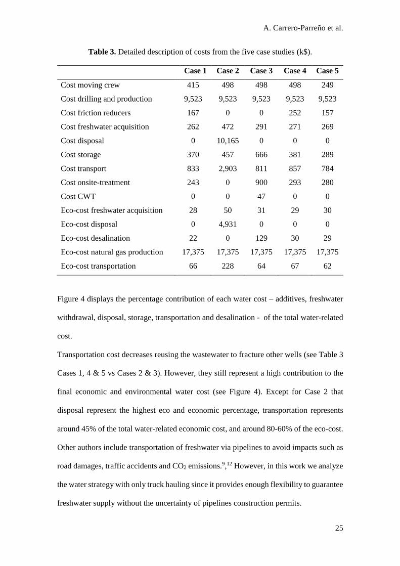
In Table 3, the different costs from the five case studies are reported in detail. Water-

related costs range from 5 to 13% for the different case studies of the revenue of shale

gas production. Regarding economics, the cost of drilling and production represents for

Cases 1, 3, 4 & 5 the highest contribution of the total cost. In Case 2, the disposal cost

yields the highest contribution in the total cost ($10,165k), however, it is close to the

drilling and production cost equal to $9,523k. Regarding the environmental criterion, the

eco-cost of natural gas production is equal to $17,375k, which is significantly higher than

the others calculated eco-cost (see Table 3).


25

Table 3. Detailed description of costs from the five case studies (k$).

Case 1 Case 2 Case 3 Case 4 Case 5

Cost moving crew 415 498 498 498 249

Cost drilling and production 9,523 9,523 9,523 9,523 9,523

Cost friction reducers 167 0 0 252 157

Cost freshwater acquisition 262 472 291 271 269

Cost disposal 0 10,165 0 0 0

Cost storage 370 457 666 381 289

Cost transport 833 2,903 811 857 784

Cost onsite-treatment 243 0 900 293 280

Cost CWT 0 0 47 0 0

Eco-cost freshwater acquisition 28 50 31 29 30

Eco-cost disposal 0 4,931 0 0 0

Eco-cost desalination 22 0 129 30 29

Eco-cost natural gas production 17,375 17,375 17,375 17,375 17,375

Eco-cost transportation 66 228 64 67 62

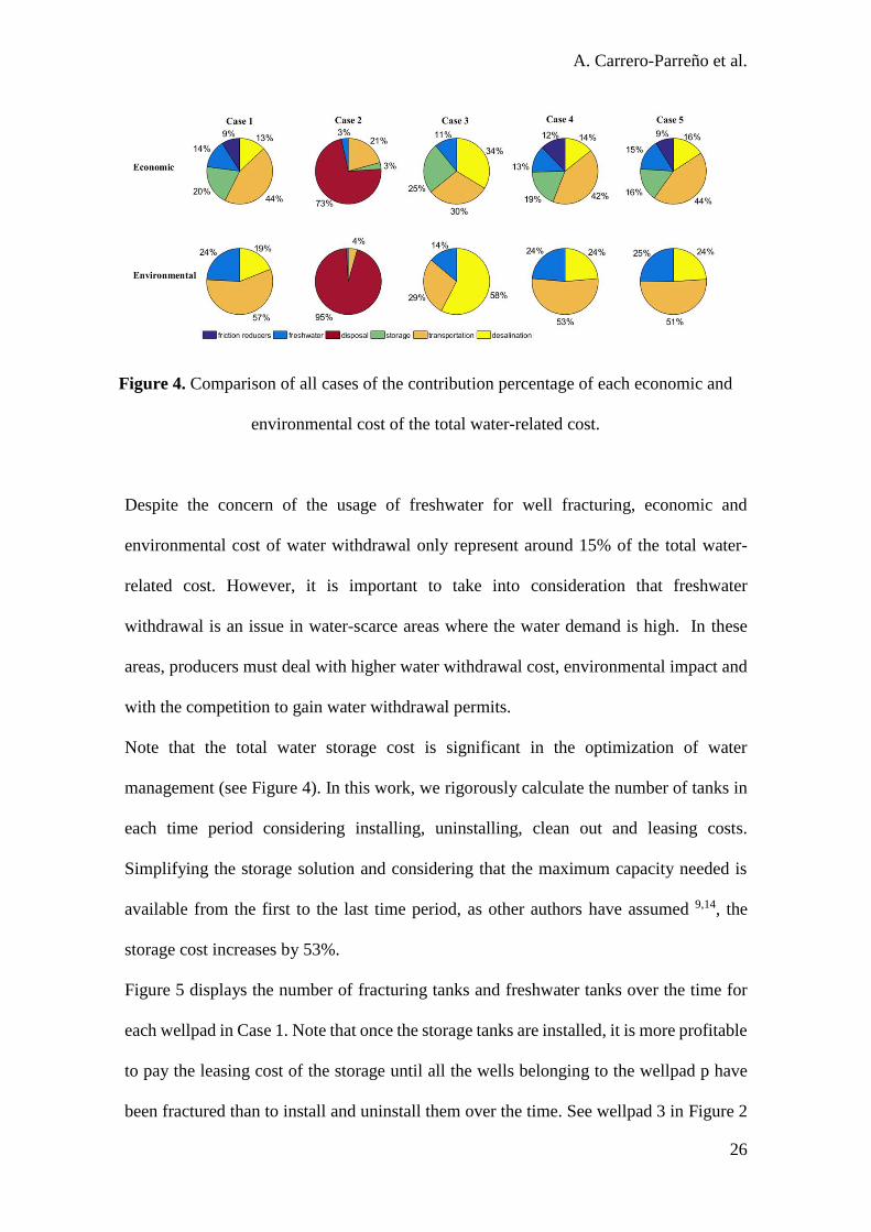
Figure 4 displays the percentage contribution of each water cost – additives, freshwater

withdrawal, disposal, storage, transportation and desalination - of the total water-related

cost.

Transportation cost decreases reusing the wastewater to fracture other wells (see Table 3

Cases 1, 4 & 5 vs Cases 2 & 3). However, they still represent a high contribution to the

final economic and environmental water cost (see Figure 4). Except for Case 2 that

disposal represent the highest eco and economic percentage, transportation represents

around 45% of the total water-related economic cost, and around 80-60% of the eco-cost.

Other authors include transportation of freshwater via pipelines to avoid impacts such as

road damages, traffic accidents and CO2 emissions.9,12 However, in this work we analyze

the water strategy with only truck hauling since it provides enough flexibility to guarantee

freshwater supply without the uncertainty of pipelines construction permits.


26

Figure 4. Comparison of all cases of the contribution percentage of each economic and

environmental cost of the total water-related cost.

Despite the concern of the usage of freshwater for well fracturing, economic and

environmental cost of water withdrawal only represent around 15% of the total water-

related cost. However, it is important to take into consideration that freshwater

withdrawal is an issue in water-scarce areas where the water demand is high. In these

areas, producers must deal with higher water withdrawal cost, environmental impact and

with the competition to gain water withdrawal permits.

Note that the total water storage cost is significant in the optimization of water

management (see Figure 4). In this work, we rigorously calculate the number of tanks in

each time period considering installing, uninstalling, clean out and leasing costs.

Simplifying the storage solution and considering that the maximum capacity needed is

available from the first to the last time period, as other authors have assumed 9,14, the

storage cost increases by 53%.

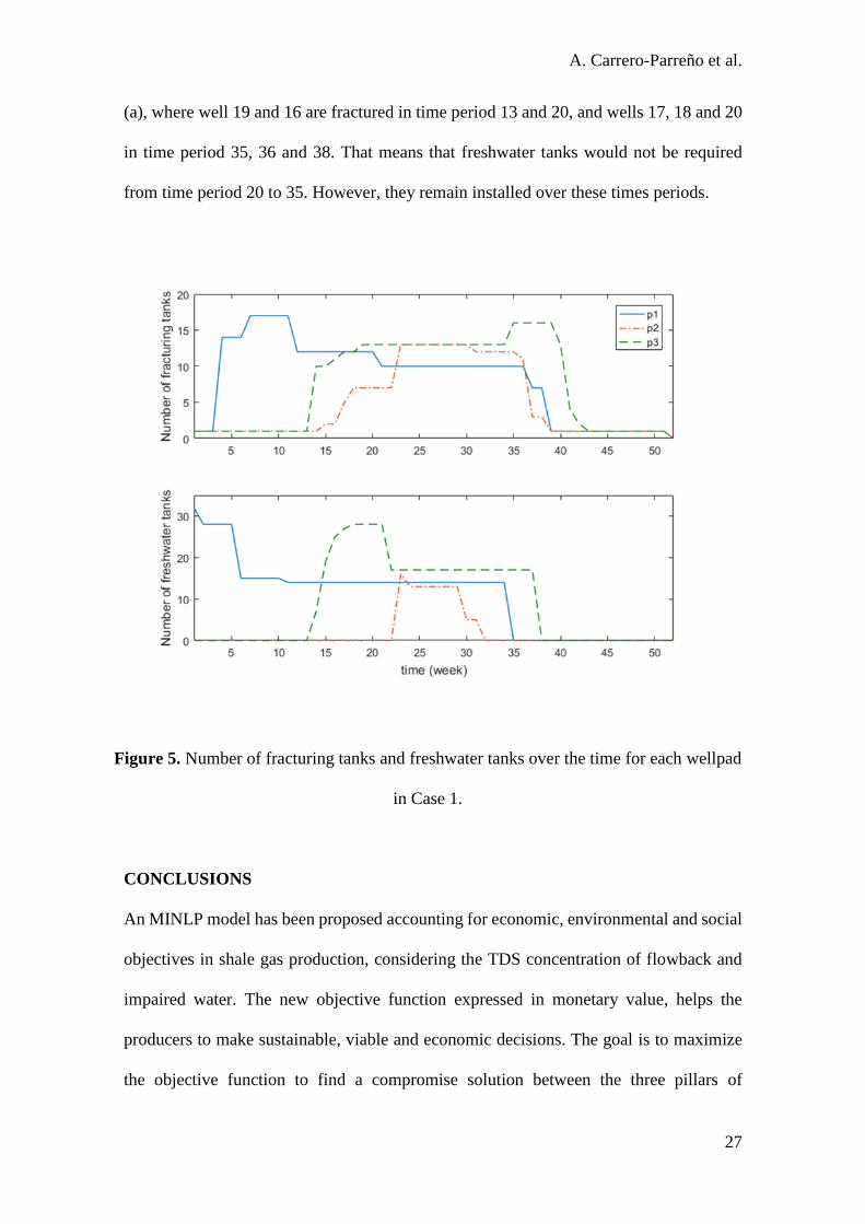
Figure 5 displays the number of fracturing tanks and freshwater tanks over the time for

each wellpad in Case 1. Note that once the storage tanks are installed, it is more profitable

to pay the leasing cost of the storage until all the wells belonging to the wellpad p have

been fractured than to install and uninstall them over the time. See wellpad 3 in Figure 2


27

(a), where well 19 and 16 are fractured in time period 13 and 20, and wells 17, 18 and 20

in time period 35, 36 and 38. That means that freshwater tanks would not be required

from time period 20 to 35. However, they remain installed over these times periods.

Figure 5. Number of fracturing tanks and freshwater tanks over the time for each wellpad

in Case 1.

CONCLUSIONS

An MINLP model has been proposed accounting for economic, environmental and social

objectives in shale gas production, considering the TDS concentration of flowback and

impaired water. The new objective function expressed in monetary value, helps the

producers to make sustainable, viable and economic decisions. The goal is to maximize

the objective function to find a compromise solution between the three pillars of


28

sustainability. The economic indicator includes revenue from natural gas and cost related

to drilling and production, storage, freshwater withdrawal, friction reducer,

transportation, disposal and treatment. The environmental indicator takes into

consideration cost of transportation, treatment, disposal, water withdrawal and shale gas

extraction. The social indicator includes social security contributions, social effects due

to the new jobs created and social cost. The inclusion of friction reducers cost function of

TDS concentration allows to determine if reusing impaired water is a cost barrier.

Additionally, the rigorous calculation of storage solution permits to operators to know the

number of tanks that should be leased in each time period.

The proposed decomposition technique solves the MINLP model effectively. First, the

original problem is relaxed using McCormick convex envelopes obtaining a relaxed

MILP. Then, the fracturing schedule is fixed, and the reduced MINLP is solved.

We have presented different case studies based on Marcellus Play. Different assumptions

are analyzed in each case study to gain a clear understanding of the nature of the problem.

The results reveal that reusing flowback water is possible to obtain a compromise solution

between economic, environmental and social criterium. The level of TDS in impaired

water is not an obstacle to reusing it for fracturing purposes, although the concentration

increases over the time, and consequently the cost of the friction reducers. Also, it has

been shown that onsite desalination treatment can be cost-effective for operators once no

more wells are available to be fractured. Finally, it should be noted that transportation is

the highest water-related contribution to both economic and environmental impacts.


29

ACKNOWLEDGMENTS

This project has received funding from the European Union’s Horizon 2020

Research and Innovation Program under grant agreement No. 640979 and from the

Spanish «Ministerio de Economía, Industria y Competitividad» CTQ2016-77968-C3-02-

P (FEDER, UE).

NOMENCLATURE

Parameters

, ,wellt p wC Concentration of flowback water forecast for well w on wellpad p in time

period t

conC Outlet salinity for desalination treatments

sCST Capacity of storage tank s

,pad disp dD −

Distance from wellpad p to disposal well d

,pad sourcef pD −

Distance from source f to wellpad p

pad offpD −

Distance from wellpad p to offsite-treatment

,pad padp ppD −

Distance from wellpad p to wellpad pp

, ,well

t p wF Flowback water forecast for well w on wellpad p in time period t

, ,,on UP on LOn nF F Maximum and minimum onsite capacity for treatment wt

,cwt UPkF Maximum centralize water treatment capacity k

, ,gas

t p wF Production gas flow forecast for well w on wellpad p in time period t

,UP LOs sN N Upper and lower bound of tanks s installed


30

, ,,im UP im LON N Upper and lower bound of impoundments installed

, ,,on UP on LON N Upper and lower bound of onsite treatment leased

imV Capacity of an impoundment

wWD Water demand of well w

w Time to fracture well w

pre Pretreatment recovery factor

rec Centralized water treatment recovery factor

drill Drilling and completion cost

prod Shale gas production cost

disd Disposal coefficient cost coefficient for disposal d

stos Storage leasing cost coefficient for storage tank s

im Impoundment construction cost

sourcef Freshwater cost coefficient in freshwater source f

fr Friction reducer cost coefficient

truck Trucking cost coefficient

reuse Pretreatment cost coefficient aiming its reuse

treat Pretreatment cost coefficient aiming its desalination

crew Cost of moving crews

onn Onsite desalination cost coefficient for treatment n

cwtk Cost coefficient of centralized water treatment k

gast Natural gas price forecast in time period t

stos Mobilize, demobilize and cleaning cost coefficient for storage tank s


31

fr Friction reducer cost coefficient

onn Maintenance cost coefficient for onsite desalination treatment n

fr Overestimated cost of friction reducers

Integer variables

, ,t p sn Number of tank type s on wellpad p on time period t

, ,inst p sn Number of tank type s installed on wellpad p on time period t

, ,unist p sn Number of tank type s uninstalled on wellpad p on time period t

,imt pn Number of impoundments on wellpad p on time period t

,,

im inst pn Number of impoundments installed on wellpad p on time period t

, ,ont p nn Number of onsite treatment n on wellpad p on time period t

,, ,

on inst p nn Number of onsite treatment n installed on wellpad p on time period t

,, ,

on unist p nn Number of onsite treatment n uninstalled on wellpad p on time period t

Binary variables

, , ,hft p w cy Indicates if well w on wellpad p is stimulating using fracturing crew c in

time period t

, ,stt p sy Indicates if storage tank type s are installed on wellpad p in time period t

, ,ont p ny Indicates if onsite treatment n is used on wellpad p in time period t

, ,crewt p cy Indicates if at least one well is drilled in wellpad p in time period t with

fracturing crew c

Variables

,padt pc Salt concentration on wellpad p in time period t


32

,t pc Salt concentration in fracturing tanks on wellpad p in time period t

,it pc Salt concentration of the inlets flows in fracturing tanks on wellpad p in time

period t

drillE Drilling and production expenses

disE Disposal expenses

stoE Storage freshwater and wastewater expenses

sourceE Freshwater acquisition expenses

frE Friction reducer expenses

transE Transport expenses

ondesE Onsite treatment expenses

cwtE Centralized water treatment expenses

drillE Drilling and production expenses

crewE Moving crew expenses

, ,well

t p wf Flowrate of produce water on well w wellpad p in time period t

,pad

t pf Flowrate of produce water on wellpad p in time period t

,,pre in

t pf Onsite pretreatment inflow in wellpad p in time period t

, ,source

t p ff Flowrate of freshwater from natural source f to wellpad p in time period t

,,on fwt

t pf Flowrate of desalinated water from onsite treatment to freshwater tanks in

wellpad p in time period t

,, ,pad fwt

t pp pf Flowrate of desalinated water from wellpad pp to freshwater tanks in



33

,,on des

t pf Flowrate of freshwater used in hydraulic fracturing in wellpad p in time

period t

,imp

t pf Flowrate of impaired water used in hydraulic fracturing in wellpad p in

time period t

,dem

t pf Flowrate of water demand in wellpad p in time period t

,,pre out

t pf Onsite pretreatment outflow in wellpad p in time period t

,,on slud

t pf Slud flowrate after onsite desalination process in wellpad p in time period t

,,on in

t pf Onsite desalination inflow in wellpad p in time period t

,,on out

t pf Onsite desalination outflow in wellpad p in time period t

,, ,on brine

t p df Brine flowrate after onsite desalination process in wellpad p in time period t

,,on fresh

t pf Flowrate of desalinated water from onsite treatment on wellpad p in time

period t sent to discharge

,,cwt in

t kf Inlet flow in centralized water treatment k in time period t

,,cwt out

t kf Outlet flow in centralized water treatment k in time period t

,, ,cwt fwt

t p kf Desalinated water from centralized water treatment k to freshwater tank on


,,cwt des

t kf Desalinated water from centralized water treatment k to discharge in time

period t

, ,i

t p sf Outlet flow in tank s in wellpad p in time period t

, ,o

t p sf Inelt flow in tank s in wellpad p in time period t


34

gasR Total gas revenue

, ,t p sst Level of water in tank type s on wellpad p in time period t

, ,fb

t p wy Indicates when the water starts to come out on well w on wellpad p in time

period t

REFERENCES

1. U.S. Energy Information Administratio. International Energy Outlook 2016.

http://www.eia.gov/outlooks. Published 2016. Accessed March 12, 2018.

2. Gao J, You F. Design and optimization of shale gas energy systems: Overview,

research challenges, and future directions. Comput Chem Eng. 2017;106:699-718.

3. U.S. Environmental Portection Agency. Technical Development Document For

Effluent Limitations Guidelines and Standars for the Oil and Gas Extraction Point

Source Category. Washington, DC; 2016.

4. Holditch SA. Getting the Gas Out of the Ground. Chem Eng Prog. 2012.

5. Mimouni A, Kuzmyak N, Oort E van, Sharma M, Katz L. Compatibility of

hydraulic fracturing additives with high salt concentrations for flowback water

reuse. In: World Environmental and Water Resources Congress 2015. ; 2015:496-

509.

6. Paktinat J, Neil BO, Tulissi M, Service TW. Case Studies : Improved Performance

of High Brine Friction Reducers in Fracturing Shale Reserviors. SPE Int. 2011.

7. Ruyle B, Fragachan FE. Quantifiable Costs Savings by Using 100 % Raw

Produced Water. . SPE Int. 2015.

8. Yang L, Grossmann IE, Manno J. Optimization models for shale gas water

management. AIChE J. 2014;60(10):3490-3501.

9. Yang L, Grossmann IE, Mauter MS, Dilmore RM. Investment optimization model


35

for freshwater acquisition and wastewater handling in shale gas production. AIChE

J. 2015;61(6):1770-1782.

10. Bartholomew T V, Mauter MS. Multiobjective Optimization Model for

Minimizing Cost and Environmental Impact in Shale Gas Water and Wastewater

Management. ACS Sustain Chem Eng. 2016;4(7):3728-3735.

11. Gao J, You F. Optimal Design and Operations of Supply Chain Networks for Water

Management in Shale Gas Production : MILFP Model and Algorithms for the

Water-Energy Nexus. AIChE J. 2015;61(4).

12. Gao J, You F. Shale Gas Supply Chain Design and Operations toward Better

Economic and Life Cycle Environmental Performance: MINLP Model and Global

Optimization Algorithm. ACS Sustain Chem Eng. 2015;3(7):1282-1291.

13. Guerra OJ, Calderón AJ, Papageorgiou LG, Siirola JJ, Reklaitis G V. An

optimization framework for the integration of water management and shale gas

supply chain design. Comput Chem Eng. 2016;92:230-255.

14. Lira-Barragán LF, Ponce-Ortega JM, Guillén-Gosálbez G, El-Halwagi MM.

Optimal Water Management under Uncertainty for Shale Gas Production. Ind Eng

Chem Res. 2016;55(5):1322-1335.

15. Lira-Barragán LF, Ponce-Ortega JM, Serna-González M, El-Halwagi MM.

Optimal Reuse of Flowback Wastewater in Hydraulic Fracturing Including

Seasonal and Environmental Constraints. AIChE J. 2016;62(5).

16. Drouven MG, Grossmann IE. Optimization models for impaired water

management in active shale gas development areas. J Pet Sci Eng. 2017;156:983-

995.

17. Zore Ž, Čuček L, Kravanja Z. Syntheses of sustainable supply networks with a new

composite criterion – Sustainability profit. Comput Chem Eng. 2017;102:139-155.


36

18. Carrero-Parreño A, Onishi VC, Salcedo-Díaz R, Ruiz-Femenia R, Fraga ES,

Caballero JA, Reyes-labarta JA. Optimal Pretreatment System of Flowback Water

from Shale Gas Production. Ind Eng Chem Res. 2017;56(15):4386-4398.

19. Carrero-Parreño A, Onishi VC, Ruiz-Femenia R, Salcedo-Díaz R, Caballero JA,

Reyes-labarta JA. Multistage Membrane Distillation for the Treatment of Shale

Gas Flowback Water: Multi-Objective Optimization under Uncertainty. Comput

Aided Chem Eng. 2017;40:571-576.

20. Onishi VC, Carrero-Parreño A, Reyes-Labarta JA, Ruiz-Femenia R, Salcedo-Díaz

R, Fraga ES, Caballero JA. Shale gas flowback water desalination: Single vs

multiple-effect evaporation with vapor recompression cycle and thermal

integration. Desalination. 2017;404(C):230-248.

21. Onishi VC, Carrero-Parreño A, Reyes-Labarta JA, Fraga ES, Caballero JA.

Desalination of shale gas produced water: A rigorous design approach for zero-

liquid discharge evaporation systems. J Clean Prod. 2017;140:1399-1414.

22. Delft University of Technology. The Model of the Eco-costs/Value Ratio (EVR).

http://www.ecocostsvalue.com. Published 2017. Accessed December 1, 2017.

23. Garth P. McCormick. Mathematical programming computability of global

solutions to factorable nonconvex programs: Part i - convex underestimating

problems. Math Program. 1976;10(1):147-175.

24. Rosenthal RE. GAMS — A User ’s Guide. GAMS Doc 246. 2016;(January):1-316.

25. Gurobi Optimization I. Gurobi Optimizer Reference Manual.

http://www.gurobi.com. Published 2016.

26. Duran MA, Grossmann IE. An outer-approximation algorithm for a class of mixed-

integer nonlinear programs. Math Program. 1986;36:307-339.

27. Drud A. CONOPT: A GRG code for large sparse dynamic nonlinear optimization


37

problems. Math Program. 1985;31(2):153-191.

28. United States Department of Labor. Usual Weekly Earnings of Wage and Salary

Workers. Bureau of Labor Statistics.

https://www.bls.gov/news.release/wkyeng.toc.htm. Accessed March 12, 2018.

29. Petroleum Services Association of Canada. How many jobs does a single drilling

rig create and where are they? Alberta Oil - The Business of Energy.

https://www.albertaoilmagazine.com/2015/05/drilling-rig-jobs/. Published 2015.

Accessed March 12, 2018.

30. Urban Institute & Brookings Institution. Tax Policy Center.

http://www.taxpolicycenter.org/taxvox. Accessed March 12, 2018.


38

APPENDIX A

The parameters used in this work are listened in the following tables.

Table A.1. Costs coefficient

Parameter Value Units Ref

Drilling cost (drill ) 270,000 $

12

Production cost (prod ) 0.014 $/m3

12

Disposal cost (disd ) 90 - 120 $/m3

9

Truck cost (truck ) 0.15 $/km/m3

9

Storage cost ( stos ) 70 $/week/tank *

Impoundment cost (im ) 3.86 $/m3

8

Pretreatment cost (reuse ,

treat ) 0.8 - 2 $/m3 18

Desalination cost (ondesn ) 6 - 15 $/m3

20,19

Demobilize, mobilize and clean out cost (ondesn ) 2,000 $/week *

Centralized water treatment (cwtk ) 42 - 84 $/m3

9

Demobilize, mobilize and clean out cost (stos ) 1,500 $ *

F Friction reducer cost (fr ) 0.18 - 0.30 $/m3 *

Freshwater withdrawal cost (sourcef ) 1.76 - 3.5 $/m3

8

Moving crew cost (crew ) 83,000 $ *

*Provided by a company


39

Table A.2. Model parameters


sCST 60 m3 *

, ,wellt p wC 3,000 - 200,000 ppm 3

conC 300 g kg-1 20

, ,well

t p wF 2,400 – 9,300 m3 week-1 3

, ,gas

t p wF 2.8 106 – 0.6 106 m3 week-1 3

,on UPnF 4,000 m3 week-1 *

,cwt UPkF 16,700 m3 week-1 *

UPsN 100 - *

,im UPN 3 - *

,on UPnN 3 - *

imV 120 m3 *

wWD 4,800 - 18,600 m3 week-1 3

w 1-5 weeks 3

*Provided by a shale gas company


40

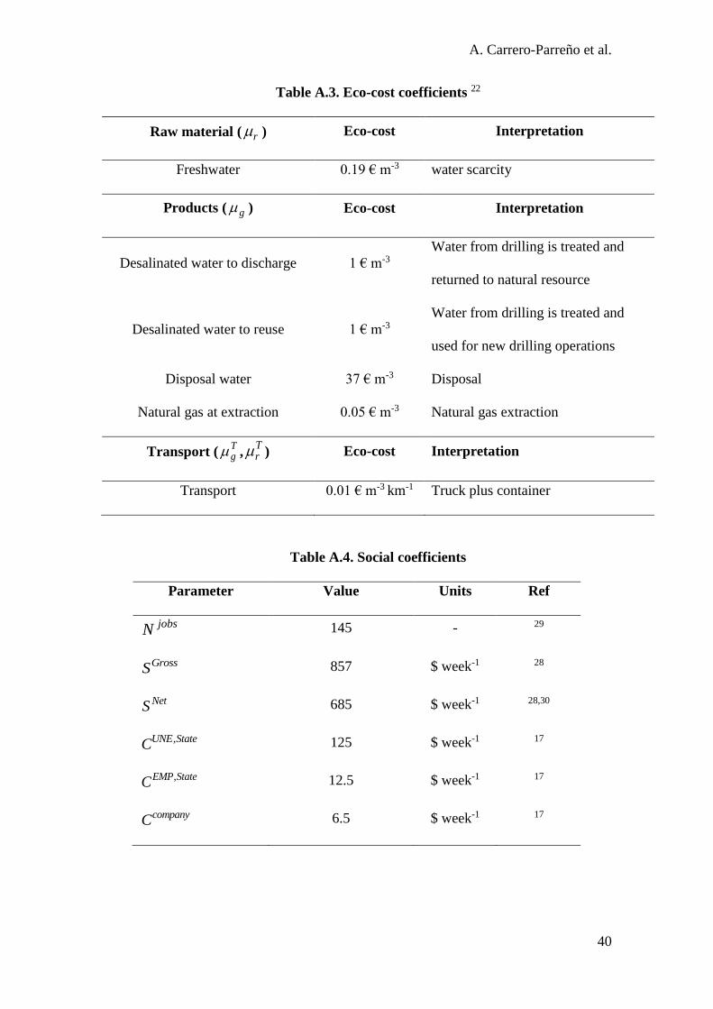
Table A.3. Eco-cost coefficients 22

Raw material ( r ) Eco-cost Interpretation

Freshwater 0.19 € m-3 water scarcity

Products ( g ) Eco-cost Interpretation

Desalinated water to discharge 1 € m-3

Water from drilling is treated and

returned to natural resource

Desalinated water to reuse 1 € m-3

Water from drilling is treated and

used for new drilling operations

Disposal water 37 € m-3 Disposal

Natural gas at extraction 0.05 € m-3 Natural gas extraction

Transport (Tg ,

Tr ) Eco-cost Interpretation

Transport 0.01 € m-3 km-1 Truck plus container

Table A.4. Social coefficients


jobsN 145 - 29

GrossS 857 $ week-1 28

NetS 685 $ week-1 28,30

,UNE StateC 125 $ week-1 17

,EMP StateC 12.5 $ week-1 17

companyC 6.5 $ week-1 17

sustainable optimal strategic planning for shale water...

Documents