Survival of Commodity Trading Advisors: Systematic vs.Discretionary CTAs.

Julia Arnold, Robert Kosowski, Paolo Za¤aroni1

Abstract: This study investigates the di¤erences in mortality between systematic and discretionary CommodityTrading Advisors, CTAs, over 1994-2009 period, the longest horizon than any encompassed in the literature. This

study shows that liquidation is not the same as failure in the CTA industry. New lters are proposed that allow

to identify real failures among funds in the graveyard database. By reexamining the attrition rate, this study

nds that the real failure rate is in fact 11.1% in the CTA industry lower than the average yearly attrition rate

of 17.3%. Secondly this study proposes a new way to classify CTAs, mainly into systematic and discretionary

funds and provides detailed analysis of their survival. Systematic CTAs are found to have higher median survival

than discretionary, 12 years vs. 8 years. The e¤ect of various covariates including several downside risk measures

is investigated in predicting CTA failure. Controlling for performance, HWM, minimum investment, fund age,

leverage and lockup, funds with higher downside risk measures have a higher hazard rate. Compared to the

other downside risk measures, volatility of returns is less able to predict failure. Fund ows have signicant and

positive e¤ect on the probability of survival, funds that receive larger inows are able to survive longer than

funds that do not. Finally larger systematic CTAs have the highest probability of survival.

Keywords: CTA failure, liquidation, median survival, attrition rate, downside risk, systematic,discretionary.

JEL Classication: G11, G12, C31

1Paolo Za¤aroni is at Imperial College Business School p.za¤aroni@imperial.ac.uk. Robert Kosowski is at Im-perial College Business School and the Oxford-Man Institute of Quantitative Finance r.kosowski@imperial.ac.uk.Julia Arnold is at Imperial College Business School and Tuneinvest Ltd.

1

2

Introduction

Over the last decade, the CTA and hedge fund industry has more than doubled in both size and

number of funds. Estimates indicate that, at its peak in the summer of 2008, the entire industry

managed around US$2.5 trillion. The impact of the financial crisis of 2008-2009, however, has

clearly been felt by the hedge fund and CTA industries. The crisis is arguably the largest in

modern financial history and has led assets under management to fall sharply via a combination

of trading losses and investor withdrawals. Although assets under management have decreased

in the hedge fund industry as a whole, they have increased slightly in the CTA industry over

the course of this crisis. BarclayHedge reports a level of assets under management for CTAs

of over US$200 billion for the end of 2009. In addition, around 50% of funds have less than

US$10 million in assets, suggesting a high number of new entrants into the industry. The rapid

growth of the CTA and hedge fund industries has also been accompanied by a growth in the

number and severity of failures, however. Investors recognize that whilst hedge funds and CTAs

may produce high expected returns they may also expose investors to potentially large downside

risks.

The term CTA represents an industry of money managers known as Commodity Trading

Advisors who accept compensation for trading on behalf of their clients in the global futures

and forwards markets. These funds originally operated predominantly in commodities markets

but today they invest in liquid futures and forwards markets in commodities, currencies, fixed

income and equity indices. CTAs are usually self-regulated and registered with the National Fu-

tures Association (NFA), a self-regulatory organization for futures and options markets. CTAs

are known to have unique risks and nonlinear returns. Fung and Hsieh (1997b) documented

CTAs to have nonlinear and non-normal payoffs due to their dynamic trading strategies and use

3

of derivatives. Some of the previous research suggests that CTAs demonstrate positive skewness

and excess kurtosis and a rejection of the Jarque-Bera (1980) test for normality.2 Like hedge

funds, CTAs charge a management fee and, in particular, an incentive fee which some have

argued may create an incentive for excessive risk taking.

An important issue for both private and institutional investors is how to best achieve a

targeted return with an acceptable level of risk. A possible solution would be a diversified

portfolio with a certain portion allocated to managed futures. Lintner (1983) showed that the

risk-adjusted return of a portfolio of stocks and bonds exhibits substantially less variance at

every level of expected return when combined with managed futures. Yet a much debated issue

remains whether managed futures have done well enough on a stand alone basis to justify the

high fees that they charge, Amin and Kat (2004), Kosowski, Naik and Teo (2007), Liang (1999),

Liang (2001) and Bhardwaj, Gorton and Rouwenhorst (2008). In order to properly address the

performance issue one needs to first account for the mortality and survivorship bias associated

with these funds. Moreover, while historically most of the money held by CTAs and hedge funds

was from high-net-worth individuals, recent growth in assets under management has been from

institutional investors such as pension plans and insurance companies. Unlike private high-net-

worth individuals, to meet their obligations institutional investors need to allocate capital on a

long-term basis with reliable return streams. Selecting alternative investments that are likely

to produce stable returns and remain in operation is, therefore, of particular interest to these

investors. Survival analysis can be useful as it can provide additional due diligence and aid the

selection of funds that are less likely to liquidate.

The study of survival in the CTA industry is sparse and in its virtual infancy. Although

2See Liang (2004), Park (1995), Edwards and Park (1996), Gregoriou and Rouah (2004), Schneeweis andGeorgiev (2002).

4

previous literature points to a higher attrition rate for CTAs relative to hedge funds, Brown,

Goetzmann and Park (2001), these studies do not take into account extreme market events,

simply due to their limited data sample. A few studies, however, have shown that CTAs provide

downside protection during bear market conditions.3 Analyzing survival during the recent fi-

nancial crisis is of particular interest to investors who have become ever more cautious investing

in hedge funds. This study provides a detailed survival analysis over a new range of CTA classi-

fications and encompasses the longest time horizon of any examined in the literature, including

the recent financial crisis of 2008.4 In doing so, it makes several contributions. The first is to

distinguish the real failure rate from the attrition rate of CTAs. By clarifying the definition of

real failure, despite the fact that to date all CTA studies have deemed the two concepts as one,

it is possible to estimate a real failure rate of the CTA industry over the longest period so far

studied. Secondly, it finds that CTA survival is heavily dependent on the strategy of CTAs.

Whilst Baquero et al. (2005) and Liang and Park (2010) find that hedge fund style is a factor

in explaining hedge fund survival, Gregoriou et al. (2005) examine survival over a range of CTA

classifications and find that survival is heavily related to the strategy of the CTA. Whilst these

authors use the CTA classifications directly provided by the BarclayHedge database, this study

makes an important contribution by reclassifying CTAs into two main trading styles: system-

atic and discretionary, and shows how survival is related to these styles. The life expectancy

of CTAs is investigated at the aggregate level and for all classifications, whilst the impact of

various variables on survival is analyzed.

Hedge fund databases provide information on live and dead funds. Funds no longer report-

3Edwards and Caglayan (2001), Fung and Hsieh (1997b) and Liang (2004).4Fung and Hsieh (2009) note that as capital flows out of the hedge fund and CTA industry at an unprecedented

rate, the attrition rate is likely to rise. The full impact of the contraction of the assets may take some time tomanifest itself however. “Consequently the liquidation statistics from the second half of 2009 are likely to beimportant in estimating survivorship bias.”

5

ing to the database are moved into the “Graveyard”. Fung and Hsieh (2002), however, point

out that not all funds listed in the graveyard database have in fact liquidated. Many stopped

reporting for a variety of other reasons, including merging with another fund, name change, etc.

Earlier studies on hedge funds and CTAs have regarded moving to the graveyard as represent-

ing liquidation and failure and the attrition rates estimated by previous research have all been

based on this classification. Defining failure is particularly challenging as it is difficult to obtain

information on the reasons for exit in respect to the defunct funds, although a few databases

do provide such information. In this regard, an important contribution offered by Rouah (2005)

was explicitly to examine fundamental differences between different types of exits in hedge fund

data. His study was implemented using the HFR database which provides three drop reason

categories: liquidated, stopped reporting and closed to new investment. As such, Rouah (2005)

study was able to examine the effect of different exit types on attrition statistics, survivorship

bias and the survival analysis of hedge funds. When liquidation only was considered the average

annualized attrition rate dropped to 3-5% and the bias associated with using only live funds

and funds that stopped reporting, the survivorship bias, increased to 4.6%.5 A recent study

by Liang and Park (2010) on hedge funds also accounts for the potential shortcomings of using

the entire Graveyard database, or even just liquidated funds, as failures. Even though some

databases provide information on liquidated funds, the authors argue that even liquidation does

not necessarily mean failure, as some funds may liquidate for other reasons. The authors, there-

fore, propose a filtering system based on fund past performance and past asset flow analysis

to distinguish failed funds from those that had voluntary closures. Using this new dataset, the

5The biases present in the hedge fund and CTA data and its effects on performance are well documentedin the literature (Ackermann, McEnally and Ravenscraft (1999), Fung and Hsieh (2000b), Diz (1999a), Brown,Goetzmann, Ibbotson and Ross (1992), Fung and Hsieh (1997b) and Carpenter and Lynch (1999)), howevernone of the previous studies have accounted for the different exit types. As such, Rouah (2005) is the first todemonstrate the effect of different exit types on survivorship bias.

6

authors reexamine the effects that contribute to real failure. To date, there are no comparative

studies for CTAs exclusively, however. Furthermore, Liang and Park (2010) explicitly exclude

managed futures from their hedge fund sample.

Early studies on CTAs regarded the entire graveyard as an indication of failure because on

average such funds had poor performance, Gregoriou (2002). The attrition rate results esti-

mated by previous studies are all based on such a classification. Thus previous literature on

CTAs suggest that they experience lower survival than hedge funds (see Brown, Goetzmann and

Park (2001), Liang (2004)). Brown et al. (2001) determine that the attrition of CTAs is 20%

versus 15% for hedge funds. Liang (2004) uses HFR data for the period 1994-2003 and estimates

that hedge funds have an attrition of 13.23% in bull markets and 16.7% in bear markets, whilst

CTAs have an average attrition of 23.5%. Getmansky, Lo and Mei (2004) also find that managed

futures have the highest average annualized attrition rate, compared to other hedge fund strate-

gies, with a rate of 14.4%. Fung and Hsieh (1997b) and Capocci (2005) also find an attrition of

19%. Spurgin (1999) notes that the mortality of CTAs reached 22% in 1994. Two recent studies

however find conflicting rates. Bhardwaj et al. (2008) found an attrition rate of 27.8% whilst

Xu, Liu and Loviscek (2010) found a substantially lower rate of 11.96%. Both studies covered

the latest period but used different databases. This could account for the difference in results.

As stressed by Xu et al. (2010), however, it is important to account for attrition rates in light

of the effect of the recent crisis on the industry.

This study extends the most recent advances in survival analysis in the hedge fund literature

to CTAs, whilst encompassing the longest time period so far studied for CTAs. To date there

appears to have been no study that has analyzed CTA attrition and survival using different exit

types. The most recent CTA survival study by Gregoriou, Hubner, Papageorgiou and Rouah

7

(2005) treats all funds in the graveyard as liquidated possibly due to the limitations of their

database. In fact the authors explicitly make a strong assumption that all funds in the database

that have stopped reporting did so due to poor returns. The authors use the BarclayHedge

database for the period 1990-2003. Unfortunately, BarclayHedge does not provide exit reasons

for many funds in the graveyard. While, this study also employs BarclayHedge, since it provides

the most extensive database of CTAs, it builds on the methodology of Liang and Park (2010) to

identify failures in the CTA graveyard. One of the key contributions of this study is to extend

the failure filters proposed by Liang and Park (2010); it shows that their two return and AUM

filters are incomplete and applies extended filters to the BarclayHedge database to reclassify the

exit types of the graveyard into those that liquidated and those that are alive but no longer

report. It also separates real failures from liquidated funds. These new criteria are based on an

examination of all available information on defunct funds. Many of the funds in the database

have been contacted to confirm their liquidation status and reason for exit. Certain information

was obtained from private commercial sources and extensive internet searches.

The second contribution of this study is to reclassify the entire CTA database into investment

styles that are more commonly used in the industry. Unlike previous research, therefore, CTAs

are separated into two distinct styles: Systematic and Discretionary. Systematic CTAs base

their trading on technical models devised through rigorous statistical and historical analysis.

Investment decisions are made algorithmically and thus all the rules are applied consistently

and there is limited uncertainty as to their application. The last decade has witnessed an in-

crease in the complexity and breadth of quantitative financial research; an increase that has

been fueled by the greater availability of financial and economic data as a result of the relentless

increase in computing power. Systematic trading that requires intensive quantitative research

8

and the use of sophisticated computer models has thus become more prevalent. Most of the

entrants into this field are trained scientists and engineers. Park, Tanrikulu and Wang (2009)

argue that systematic traders may hold significant advantages over discretionary traders. Even

though discretionary traders may also follow trends they still base their trading decisions on

manager discretion. Thus one of the challenges facing discretionary traders is the control of

human emotion in reacting to difficult market conditions. Systematic programs do not have

this weakness as all the trades are executed by the program. In addition there is a lesser “key

man risk” which tends to be associated with discretionary traders. Due to their automated

nature, systematic funds have the further advantage of scalability across a multitude of markets

and they can thus accept more capital whilst allowing for more diversification across markets,

strategies employed and number of trades. In light of these differences, it is of interest to test

empirically the survival rates associated with the two strategies. A recent study by Kazemi

and Li (2010) also classifies CTAs into these two manager categories and finds that there are

differences in the market timing abilities of systematic and discretionary CTAs, notably that

systematic CTAs are generally better at market timing than discretionary CTAs. This study

however, further breaks systematic funds into sub-strategies. Park, Tanrikulu and Wang (2009)

note that systematic CTAs are comprised of multiple strategies most of which can be classified

as either trend-following or relative value. Others employ trading models that fall into neither of

these categories, e.g. pattern recognition and counter trend. Trend-following strategies are also

split into programs that primarily use short-term, medium-term or long-term signals or holding

periods. Based on the previous research, one would expect the findings of this study to indicate

that systematic CTAs have better performance and higher survival than discretionary funds,

since the lack of the human emotion element allows for better risk control and a consequent

9

reduction in the risk of failure.

Using the classification of investment styles and the failure filtering system discussed above,

the average annual attrition rate of the entire CTA database is found to be 17.3% for the 1994-

2009 period, i.e. similar to previous studies. The failure rate, however, is significantly lower at

11.1%. There are also differences between systematic and discretionary funds, with systematic

funds having lower attrition and failure rates of 16.0% and 10.4% versus 21.6% and 12.6% re-

spectively. The BarclayHedge database contains a significant number of funds with less than

US$10 million under management. After removing such funds, the average attrition and failure

rates drop to 7.8% and 4.1% for systematic and 10.8% and 5.9% for discretionary funds. These

are lower than previously estimated but comparable to the findings of Rouah (2005) and Liang

and Park (2010) for hedge funds. The results suggest that the attrition rate of CTAs may not

be as high as previously suggested and in particular systematic CTAs have a lower attrition rate

than discretionary CTAs.

Survival analysis is then implemented to determine factors affecting CTA failure. There are

a few studies in the hedge fund literature analyzing the effect of various variables on survival,

including: Liang (2000), Brown, Goetzmann and Park (2001), Gregoriou (2002), Baquero, Horst

and Verbeek (2005), Rouah (2005), Ng (2008) and Baba and Goko (2009). In particular Brown,

Goetzmann and Park (2001) find that hedge fund survival depends on absolute as well as relative

performance, seasoning and volatility. Recently, Brown, Goetzmann, Liang and Schwarz (2009)

estimated the effect of operational risk on hedge fund survival. Using novel data from SEC filings

(Form ADV) in combination with the TASS database, the study developed a quantitative model,

the ω-score, to quantify operational risk and use it as a predictor in the Cox (1972) proportional

hazards model to predict its effect on hedge fund survival. The study included managed futures

10

as a sub-strategy but found that the coefficient of operational risk was insignificant for managed

futures and the direction of its effect was blurred. The score was related to conflict-of-interest

issues, concentrated ownership and reduced leverage, none of which seem to explain CTA sur-

vival. Other studies on CTA survival are rather sparse, Diz (1999a), (1999b), Spurgin (1999)

and Gregoriou et al. (2005) each analysed CTA survival separately from hedge funds. The most

recent of these analyses is that of Gregoriou et al. (2005) who find that performance, size and

management fees have an effect on CTA survival. The influence of volatility appears rather

limited.

The particular contribution of this study is to employ downside risk measures that incorpo-

rate higher return moments in predicting CTA failure. In doing so it incorporates time varying

as well as fixed covariates. The methodology closely follows that of Liang and Park (2010), who

show that these measures are better able to capture the non-normality of hedge fund returns.

Incorporating additional risk measures is of particular interest in respect to CTAs who have

positive skewness yet can experience large losses. Drawdown as a risk measure is also considered

since this can be useful in predicting failure. Lang, Gupta and Prestbo (2006), in fact, argue

that drawdowns are the single most significant factor that determines the likelihood of hedge

fund survival. Another contribution of this study is to employ Cox (1972) proportional hazard’s

model with time-varying covariates. This is an improvement to the Gregoriou et al. (2005)

model for CTAs who employ Cox’s (1972) proportional hazard model with fixed covariates only.

By using time dependent covariates new risk measures as well as other covariates are allowed

to change with time. Finally, the aim of the study is to build a forecasting model with better

warning signals for possible fund liquidations. In order to do this as accurately as possible, the

survival analysis for three different definitions of failure is compared: i) attrition, ii) liquidation

11

and iii) real failure. The results show that standard deviation is not an appropriate risk measure

in predicting the type of failure and that downside risk measures are better able to explain real

failure. As a result, this study finds that systematic CTAs should be favoured by investors due

to their significantly higher survival than their discretionary counterparts.

The rest of the study is organized as follows. Section 1.2 describes the data. Section 1.3 ex-

plains the methods. Section 1.4 provides the empirical results and robustness tests and section

1.5 concludes.

Data

There are several databases that collect data on CTAs. The most commonly used databases in

academic studies are TASS, CISDM and BarclayHedge. To analyze the attrition and survival

of CTAs properly this study uses monthly net-of-fees returns from live and dead CTAs that re-

ported to the BarclayHedge database, proprietor of one of the most comprehensive commercially

available databases of CTAs and CTA performance. The sample period under examination in

this study is from January 1994 to December 2009, a total of 192 months: a time period that

spans both bull (pre 2000 and 2003-2007) and bear markets, such as the bursting of the tech

bubble in the spring of 2000 and, importantly, the financial crisis of 2007-2009. This constitutes

the longest period used to date to examine CTA survival. BarclayHedge provides a variety

of information other than performance. It collects fund names, management company, AUM,

minimum investment, start and ending dates, investment style, management and incentive fees,

HWM, leverage, fund status, share restrictions, and others. It is important to note that all the

information contained in these databases is reported on a strictly voluntary basis only.

The BarclayHedge database consists of both active “Live” and “Defunct” funds. The database

12

is divided into two separate parts: “Live” and “Graveyard” funds. Funds that are in the live

database are ones that are still operating and continue to provide updates on their performance.

Once a fund stops reporting for three consecutive months, the fund is moved into the Graveyard.

A fund can only be in a Graveyard once it has been listed in the live database. As of the end

of December 2009, there were 3436 funds in the combined database. Out of these, 1,016 were

live funds and 2,420 were defunct funds. The majority of the funds report their returns net of

management and incentive fees. We eliminate from our sample funds that report quarterly or

gross returns, a total of 15 funds. We also remove various long only funds and index trackers,

duplicate entries due to multiple share classes, onshore and offshore vehicles, leveraged versions

and various feeder structures and funds born prior to 1994.6 This leaves 696 live funds and 1750

defunct funds. We also remove all multi-manager funds. In words of Liang (2005), “Combining

CTAs with funds that manage several CTAs would not only cause double counting problem but

would also hide the differences in fee structures between CTAs and fund-of-funds.” To eliminate

backfill bias, for the empirical analysis we impose an additional filter in which we require funds

to have at least 24 months of non-missing returns.

Style Classification

Hedge funds are not allowed to solicit the general public, therefore detailed strategy information

is not included in the databases. In addition, several data vendors like TASS do not include

fund identities in their academic versions making it impossible to collect information on funds

from other sources. In this study, however, we had access to fund identities that allowed us to

6Figure 1.1 was constructed using all the share classes and onshore and offshore vehicles so as to capture totalassets under management accurately across the industry.

13

access information through fund websites, other sources such as Alphametrix, as well as private

sources, to get a fuller understanding of each fund’s strategy. Narang (2009) and Rami (2009)

also provided a basis to understand the complexities of the different CTA strategies. This has

allowed us to segregate CTA funds into various strategies. We therefore used funds’ self-reported

strategy description in addition to BarclayHedge categories and hand collected information and

are therefore the first to classify CTAs in this manner.

BarclayHedge classifies funds into several investment styles. There is currently no universally

accepted form with which to classify CTAs into different strategy classes. There is some form

of consensus emerging in the literature as to how best to classify various hedge fund strategies,

however nothing similar yet exists for CTAs. In fact, most of the earlier literature treated CTAs

as a single group. Recently, some studies classified CTAs into different investment styles but

these have all done so in a different manner. Gregoriou et al. (2005) grouped the BarclayHedge

classifications into five categories, yet in their 2010 paper the same authors arrived at twelve clas-

sifications from the same database. Capocci (2005), meanwhile, grouped the same dataset into

ten classifications. All of these authors have used the BarclayHedge database yet have created

different strategy classes. It is also unclear how previous studies arrived at their classifications

since most funds in BarclayHedge would frequently fall into several categories representing trad-

ing style and asset class utilized. For example, a fund may select itself to be both systematic

and technical diversified, yet the authors would have both of these as a separate category. In

this study therefore, we propose a different CTA style classification based on the one used in the

industry.

Firstly, we note that almost all funds fall into one of the three main categories based on their

self-reported trading strategies: i.e. systematic, discretionary and options strategies. Systematic

14

traders systematically apply an alpha-seeking investment strategy that is specified based on ex-

haustive research. This research is the first step in the creation of a systematic trading strategy.

As a result, most new entrants into the industry are trained scientists and engineers. Market

phenomena are uncovered with statistical analysis of historical data. Trading algorithms are

then constructed to exploit the markets and these are applied consistently. Discretionary CTAs,

on the other hand, base their models on manager’s discretion. There are several advantages of

systematic trading over the discretionary style. Firstly, the emotional element of discretionary

trading is removed. Discretionary traders may frequently suffer from disposition effect, as doc-

umented by Shefrin and Statman (1985): they are quick to realize gains and are slow to realize

losses. In essence the main difference between the two always lies in how an investment strategy

is conceived and implemented rather than what the strategy actually is. Systematic trading

takes emotion out of investing and imposes a disciplined approach. Additional benefits are re-

duction of key man risk, scalability and more diversification in terms of the number of markets

analyzed and the types of strategies employed. We separate options strategies into a separate

group as we believe they follow substantially different trading strategies compared to systematic

and discretionary funds. In particular, options funds engage in either selling options or exploit-

ing arbitrage opportunities using options. Our final three main category classification therefore

has systematic, discretionary and options CTAs. Our classification is in line with recent work

of Kazemi and Li (2010) who break their CISDM database into systematic and discretionary

CTAs. However, we further their work by breaking systematic funds into several categories:

trend-following, pattern recognition and relative value. Trend-following funds are further broken

into short-term, medium-term and long-term traders. Billingsley and Chance (1996) also sepa-

rate CTAs into technical and non-technical funds, where technical funds essentially mirror the

15

systematic funds classified in this study. The authors further note that among those technical

funds, the majority are indeed trend-followers.7 About ten percent of the funds in our database

have no BarclayHedge classification, yet when reading their detailed strategy description it is

apparent that they still fall into one of the three main categories.

The final count and description for the different investment styles are shown in the Appendix.

It is clear from the table that the representation of the investment style is not evenly distributed.

Systematic CTAs account for 60% of all CTAs. This is a lower number than the one reported

by BarclayHedge, which cites that approximately 80% of all CTAs are systematic. We have

employed a more stringent approach to qualify the funds as being systematic, however, and this

explains the lower figure in our study. Our classification results should still be treated with

caution. Due to the nature of the industry and the lack of full information, it is impossible

to arrive at strategy assessments with absolute certainty since one is relying on the managers’

statements. We also note that among systematic funds, trend-following is the most dominant

strategy with 87% of the funds. The vast majority of trend-followers employ a medium-term

frame in a variety of markets. We define short-term as anything between high frequency trading

to trades within one week. Indeed high frequency trading has become a popular strategy in

the last few years. Medium-term trend-followers are defined as those that use two weeks up to

one month trading signals and long-term trend-followers as anything above one month. Among

discretionary funds, most utilize either technical or a combination of technical and fundamental

approaches. In addition, most funds trade in diversified markets. The Appendix provides a

detailed description of strategies.

7Fung and Hsieh (2001) show that a simple trend following strategy can be modeled using look-back straddlesthat generate a non-linear payoff structure.

16

Distinguishing Discontinuation from Death and Failure

Within those funds assigned to the graveyard database, distinguishing between liquidated funds

and those that are in fact still in operation is complicated by the lack of detailed information

available on defunct hedge funds. Early studies on hedge funds regarded moving funds to the

graveyard as a de facto indication of failure. Attrition rate calculations and survival analysis

done by previous research is based on just such a broad classification. Recently, however, data

vendors began to provide information on reasons for exit. Thus, the TASS database has seven

distinct exit classifications: fund liquidated, no longer reporting, unable to contact the manager,

closed to new investment, merged into another entity, dormant, unknown. HFR, meanwhile, has

only three categories. BarclayHedge only began collecting this information very recently. As a

result, this information is only available for a small proportion of funds, the rest are classified

as unknown.8 This is in sharp contrast to other databases such as TASS or HFR. For exam-

ple, Baquero, Horst and Verbeek (2005) used the TASS database and had only a small number

of funds with an unknown disappearance reason. Rouah (2005) used the HFR database and

was able to report exit information for most funds. In this study we employ the BarclayHedge

database, however, as it has the advantage of having the widest coverage of CTAs available.

The limited nature of its information on exit types, however, renders any meaningful survival

analysis all but impossible. To circumvent this problem several studies have proposed various

methods to filter for liquidated funds in other databases as well. Baquero, Horst and Verbeek

(2005) follow Agarwal, Daniel and Naik’s (2004) quarterly flow analysis to make an assessment

of the death reason in the TASS database. Their analysis, however, concentrates on liquidation

only. Liang and Park (2010), (henceforth, LP) further make a distinction between liquidation

8Out of 2076 funds in the graveyard, only 435 funds have a recorded reason for not reporting.

17

and real failure and argue that the classification provided by the databases is not sufficient. Not

all liquidated funds fail. Some funds may choose to liquidate based on the market expectations

of managers, funds merging, or simply the manager retiring. As a consequence, LP reclassify

the database using a performance and fund flow filter system. Utilizing only failed funds they

are able to examine the effects that contribute to hedge fund failure.

Survival analysis necessitates clear definition of failure. Rouah (2005) argues that including

all the graveyard funds in the database can blur the effect of predictor variables in a survival

analysis. We filter all the funds following the three criteria used by LP: all funds in the grave-

yard, funds with negative average rate of return in the last 6 months, funds with a decrease in

assets under management (henceforth, AUM) for the last 12 months. This study finds that these

filters would miss some of the liquidated and failed funds. In particular it failed for many small

funds in our sample and for many funds that had experienced large losses more than 12 months

before the end of data.

Case 1. A failed fund with small AUM.

We found that our sample contained a lot of funds with assets under management of less than

US$20 million. Figure 1.1 shows the evolution of AUM in the CTA industry.

[Please insert Figure 1.1 here]

In fact, on average 96% of the total AUM of the industry is managed by funds with assets above

US$20 million, yet funds with less than US$20 million under management comprise almost 70%

of the total number of funds in our database. Kosowski et al. (2007) argue that funds with

less than US$20 million AUM should be excluded from the analysis due to concerns that such

funds may be too small for institutional investors. Given the large proportion of these funds

18

in the sample, removing them would greatly reduce the available data. In addition, this study

is concerned with establishing attrition and failure rate which necessitates inclusion of all the

available data. For the survival model, however, it would be sensible to remove all the funds

below the US$20 million threshold.

Figure 1.2 shows an example of Fund A, a liquidated fund with small AUM. The AUM of

Fund A remained stable during the twelve months prior to dissolution yet, in terms of downside

risk measures, the fund has failed: it had negative average return in the last six and twelve

months. Liquidation for small funds is likely to happen quickly without noticeable decline in

assets, therefore it would be impossible to filter for these funds using AUM criteria.

[Please insert Figure 1.2 here]

Case 2. Assets lost more than 12 months before end of data.

LP’s filters assume very recent failures. Some funds. however, may experience large drawdown

followed by loss of assets as investor confidence fails. Still, some funds would continue to report

to the database with virtually no assets and good returns until they finally exit. Fund B in

Figure 2 is an example of a liquidated fund that continued to report after a large drawdown and

loss of assets. LP’s criteria would be unable to identify this failure as it happened prior to 12

months before dissolution.

[Please insert Figure 1.3 here]

Case 3. Failure with positive average return in the last six months.

Some funds fail and liquidate yet in the last six months may report a positive average return

as they reduce volatility in expectation of liquidation. There is an indication that these funds

still continue to report to the database before they eventually shut down. Figure 1.4 shows an

19

example of fund C with a negative annualized compound rate of return, with a loss in AUM, yet

it has an positive average rate of return in the last six months.

Case 4. Failure due to a large drawdown 24 months before liquidation.

Fund C is an example of a large fund that suffered a 78% drawdown and lost a majority of its

assets, yet it had a positive average return in the last six months. Such a fund would not be

picked up by LP’s criteria yet it is a clear failure and should be included in the survival model.

[Please insert Figure 1.4 here]

Ng(2008) proposes more a extensive range of filters to identify failures among hedge funds,

including the change in AUM 24 months prior to dissolution and the average return in the last

12 months. As has already been mentioned, data in this study is more limited than that used in

previous survival analyses since BarclayHedge does not provide reasons for exit for most funds.

This study, therefore, separates the graveyard into funds that are still alive but stopped reporting

and liquidated funds. It then sorts liquidated funds into those that failed and funds with various

discretionary closures. This study follows Agarwal, Daniel and Naik’s (2004) AUM flow analysis

to make an assessment of the liquidation. Fung et al. (2008), meanwhile, group liquidated funds

based on the relative AUM at the end of the fund’s life, compared to maximum AUM. We used

several filters as it is clear from looking at the previous studies that it is unlikely that one filter

can capture all the liquidated funds. In particular we filter for liquidated funds using either of

the following criteria:

• Funds with decreased AUM in the last 12 months

• Funds with decreased AUM in the last 24 months

• Funds with very low final AUM relative to the maximum AUM over the fund’s lifetime -

20

I use a 70% drop as well as a 60% drop for robustness check

• Funds with AUM equal to 0 in the last month

From the above we obtain two groups of funds; liquidated and not liquidated. Funds that are

classified as liquidated by the first set of filters are further sorted into failures or discretionary

closures. In particular we calculate the following statistics for all funds and apply them to the

“liquidated” set:

• CUM, Annualized cumulative rate of return

• Average return in the last 6, 8, 12 and 24 months

• Annualized standard deviation over entire fund history

• Drawdown in the last 12 and 24 months

Funds that had either negative average returns in the last 6, 8, 12 or 24 months, or negative

annualized cumulative returns or a drawdown in the last 12 or 24 months that was significantly

higher than annualized standard deviation were classified as Liquidated Failure. The rest of the

funds were classified as Liquidated Discretionary Closures. These are the funds that liquidated

for other reasons than bad performance as described in Liang and Park (2010). To test our

filtering we contacted many of the funds either by phone or email. The majority of the funds

that liquidated but did not experience bad returns were funds that were merging into another

fund in the same management company, funds that were going through restructuring or simply a

name change, or even retirement of the principal. Hence, these funds would affect the calculation

of the liquidation rate but they would not enter into the failure rate. We also checked funds that

did not pass the liquidation filters. In many cases these were the funds that had too small an

21

asset base to show a drop in assets but upon contacting them and looking at their returns it was

still apparent that they liquidated. There were also some funds that showed no decline in assets

nor passed any of the return filter criteria - these were funds that were still active but stopped

reporting to the database. Compared to the hedge fund industry the proportion of such funds

is not as large, possibly because CTAs would not suffer from the same capacity issues as many

hedge funds do.

Covariates & Basic Data Description

The covariates used in the survival model include average millions managed, performance, fund

age, size, lock-up provision, size volatility, and risk measures as proposed by Liang and Park

(2010). This study also adds drawdown to the risk measures. Table 1.1 presents the statistical

summary of the data for 2446 funds. The average monthly rate of return is 1.01% with a stan-

dard deviation of 6.09%. At the same time the average skewness is positive at 0.33 and average

kurtosis is 2.61. This is in contrast to the reported statistics for hedge funds found in Liang

and Park (2010) where the mean hedge fund return was 0.62%, negative skewness (-0.04) and

kurtosis 5.57. Consistent with previous literature, Table 1.1 shows that live funds outperform

defunct funds (“Graveyard funds”) with a higher standard deviation on average. The graveyard

funds also have slightly higher maximum and lower minimum returns than live funds, consistent

with higher volatility of the defunct funds. In addition, Table 1.1 shows the need to separate the

exit types. Graveyard funds are further broken into liquidated funds and funds that are alive

but stopped reporting: “Not reporting funds”. Liquidated funds have significantly lower mean

monthly returns than funds that simply stopped reporting to the database. This underlines the

fact that not all funds exit due to liquidation. The not reporting funds are also more positively

22

skewed with lower kurtosis than liquidated funds. In turn, as underlined earlier, not all liquida-

tions are indeed failures as reported in the literature. In line with this, Table 1.1 also reports

descriptive statistics for failures and discretionary closures. Real failures have the lowest mean

monthly return of 0.50% with the largest standard deviation of 6.91% and lowest skewness of

0.25. The discretionary failures have a mean return that is higher than that of the live funds

of 1.52% but lower than funds that simply stop reporting. We find that on average 41.9% of

CTAs reject the null hypothesis of normality at the 5% level. Malkiel and Saha (2005) find that

both managed futures funds and global macro hedge funds do not reject the Jarque-Bera test of

normality.9

Methodology

Risk Measures

Standard Deviation. For each month starting January 1994, we estimate standard deviation

using 60 month rolling windows of previous returns. Where 60-month data is not available a

minimum of 24 months is used.

In what follows the discussion here follows closely that in Liang and Park (2010).

SEM - Semi-deviation - this measure is similar to standard deviation except that it consid-

9See Jarque and Bera(1980).

23

ers deviation from the mean only when it is negative.

SEM ≡√

Emin[(R− µ), 0]2, (1)

where µ is the average return of the fund. SEM has been found to be a more accurate measure

for assets with non-symmetric distributions, Estrada (2001).

VaR - Value-at-Risk - is a risk measure widely used by portfolio managers which provides a

single number for the risk of loss on a portfolio. This measure allows one to make a statement

of the following form: We are (1-α) percent certain that we will not lose more than VaR(α,τ)

dollars in τ days. Thus VaR uses two parameters: the horizon (τ), and the confidence level,

(1-α). I use a 95% confidence level (α=0.05). The frequency of the data dictates the time hori-

zon, which is monthly in this case. In particular, the VaR statistic can be defined as a one-sided

confidence interval on a portfolio loss:

Prob[∆P (∆t,∆x) > V aR] = 1− α, (2)

where ∆P (∆t,∆x) is the change in the market value of the portfolio, as a function of the time

horizon ∆t and the vector of changes of random variables. This formulation shows that the

distribution of the portfolio returns is key. Calculation of the true distribution is generally not

feasible. VaR can be estimated using parametric techniques, however most assume normally

distributed returns. The VaR measure under this normality assumption becomes:

VaR Normal(α) = −(µ+ z(α)× σ) (3)

24

VaR CF - The Cornish-Fisher (1973) expansion (V aR CF ) considers higher moments in

the return distribution such as skewness and kurtosis. It is possible to obtain an approximate

representation of any distribution with known moments in terms of any known distribution,

for example normal distribution. Thus the Cornish-Fisher expansion explicitly incorporates

skewness and kurtosis, making it particularly suitable for use with CTA data. The equations

below explicitly show the terms in the Cornish-Fisher (1937) expansion.

Ω(α) = z(α) +1

6(z(α)2 − 1)S +

1

24(z(α)3 − 3z(α))K − 1

36(2z(α)3 − 5z(α))S2 (4)

V aR CF (α) = −(µ+ Ω(α)× σ) (5)

where µ is the average return, σ is the standard deviation, S is the skewness, K is the excess

kurtosis of the past 24− 60 monthly returns of CTAs, (1− α) is the confidence level, and z(α)

is the critical value from the standard normal distribution.

ES - Expected Shortfall - Another measure of risk that is included in the analysis is the

expected shortfall, ES. Artzner, Delbaen, Eber and Heath (1999) argue that ES has superior

mathematical properties to VaR. Liang and Park (2007) formally test this for hedge funds and

confirm that expected shortfall is better able to explain the cross-section of hedge funds. Unlike

VaR, ES tells us how big the expected loss could be once VaR is breached. It is therefore more

sensitive to the shape of the loss distribution in the tail of the distribution. ES is the conditional

expected loss greater or equal to VaR, sometimes called conditional value at risk. It can be

25

defined in terms of portfolio return instead of notional amount and is defined as follows:

ESt(α, τ) = −Et [Rt+τ |Rt+τ ≤ −V aRt(α, τ)]

= −

−V aRt(α,t)∫v=−∞

vfR,t(v)dv

FR,t[−V aRt(α, τ)]

= −

−V aRt(α,t)∫v=−∞

vfR,t(v)dv

α(6)

where Rt+τ denotes portfolio return during periods t and t+τ , and fR,t is the conditional proba-

bility density function (PDF) ofRt+τ . Here, FR,t denotes the conditional CDF ofRt+τ conditional

on the information available at time t, F−1R,t, and 1−α is the confidence level. To compute 95%

ES using the Cornish-Fisher expansion, one needs to compute 95% VaR CF based on equation

(1.4) and (1.5) and then search through the 60-month returns window to find all the returns

that are below the calculated 95% VaR. The average of the obtained returns is ES CF with a

95% confidence level. Alternative way is to use the analytical solution due to Christoffersen and

Goncalves (2005). However, Liang and Park (2010) show that due to extreme skewness of some

of the hedge funds the analytical solution is not very applicable.

TR - Tail Risk - Tail Risk is known as the possibility that an investment will move more

than three standard deviations from the mean and this probability is greater than that shown

by normal distribution. Tail risk arises for assets that do not follow normal distribution. In this

context, tail risk is the standard deviation of the losses greater than VaR from the mean, or,

26

more formally:

TRt(α, τ) =√Et[(Rt+τ − Et(Rt+τ ))2|Rt+τ ≤ −V aRt(α, τ)] (7)

Note that TR CF denotes Tail Risk estimated using VaR CF as a cut-off criteria.

Maximum Drawdown - Drawdown is any losing period during an investment record. It

is defined as the percent retrenchment from an equity peak to an equity valley. A drawdown

is in effect from the time an equity retrenchment begins until a new equity high is reached

(i.e. In terms of time, a drawdown encompasses both the period from equity peak to equity

valley (Length) and the time from the equity valley to a new equity high (Recovery). Maximum

Drawdown is simply the largest percentage drawdown that has occurred in any investment data

record. Diz (1999b) analyses the effect of various variables on the probability of survival of CTAs

and includes maximum monthly drawdown as one of the covariates. He finds that the maximum

monthly drawdown and the maximum time to recover from a drawdown as a percentage of a

program’s life is negatively related to survival. Baba and Goko (2009) explicitly model time

varying drawdown in their survival model of hedge funds only and come to the same conclusion.

Maximum Drawdown relative to Standard Deviation - we also calculate drawdown relative to

annualized standard deviation. Annualized standard deviation is given by:

St.Dev.Annualised =

√√√√(∑N

i=1(Ri − µR)2

N − 1

)× 12

12

(8)

27

The proportion is calculated as:

=Max.Drawdown

Std.Dev.Annuliased(9)

Once the drawdown reaches two times annualized standard deviation the fund is unlikely to

survive.

Survival Analysis

Survival analysis is concerned with analyzing the probability and time until some event occurs.

Such events are typically referred to as failures. In this context, failures are defined as financial

distress of CTAs. In the literature the problem of hedge fund survival and variables that affect

it is addressed by the use of hazard models. The underlying setting of these is as follows. If we

denote T as a nonnegative continuous random variable representing time to failure of a CTA.

The cumulative probability distribution is given by:

F (t) = Pr(T ≤ t) (10)

F(t) is also known in the literature as the failure function. An alternative formulation, which is

at the core of the survival analysis, is the survivor function: an elapsed time since the entry to

the state at time 0. This is given as:

S(t) = 1− F (t) = Pr(T > t) (11)

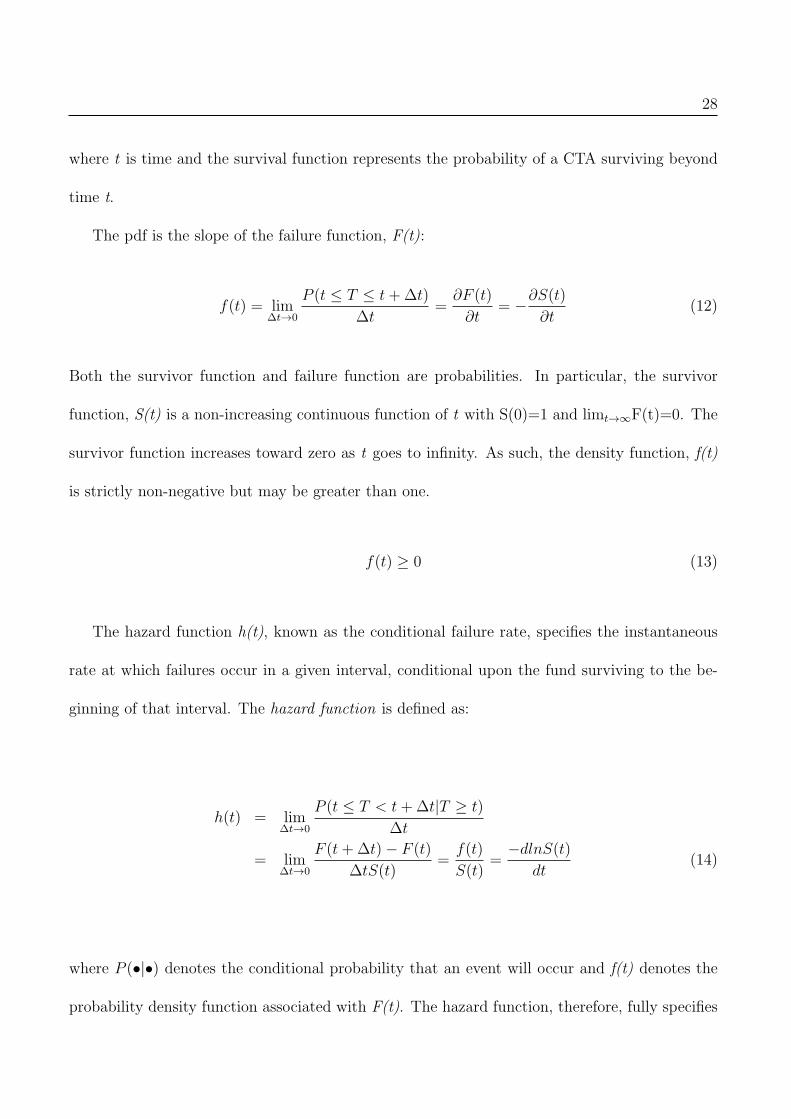
28

where t is time and the survival function represents the probability of a CTA surviving beyond

time t.

The pdf is the slope of the failure function, F(t):

f(t) = lim∆t→0

P (t ≤ T ≤ t+∆t)

∆t=

∂F (t)

∂t= −∂S(t)

∂t(12)

Both the survivor function and failure function are probabilities. In particular, the survivor

function, S(t) is a non-increasing continuous function of t with S(0)=1 and limt→∞F(t)=0. The

survivor function increases toward zero as t goes to infinity. As such, the density function, f(t)

is strictly non-negative but may be greater than one.

f(t) ≥ 0 (13)

The hazard function h(t), known as the conditional failure rate, specifies the instantaneous

rate at which failures occur in a given interval, conditional upon the fund surviving to the be-

ginning of that interval. The hazard function is defined as:

h(t) = lim∆t→0

P (t ≤ T < t+∆t|T ≥ t)

∆t

= lim∆t→0

F (t+∆t)− F (t)

∆tS(t)=

f(t)

S(t)=

−dlnS(t)

dt(14)

where P (•|•) denotes the conditional probability that an event will occur and f(t) denotes the

probability density function associated with F(t). The hazard function, therefore, fully specifies

29

the distribution of t and subsequently the density and survivor functions. The only restriction

on the hazard rate implied by the properties of these functions is that:

h(t) ≥ 0 (15)

Thus λ(t) may be greater than one, in the similar way that f(t) may be greater than one. In fact

there is a key relationship between these functions that underpins much of the survival analysis.

Whatever the functional form for the hazard rate, λ(t), one can derive the survivor function

S(t), failure function F(t) and integrated hazard rate H(t) from it. In particular from (11) and

(13) we obtain:

h(t) =f(t)

S(t)

=f(t)

1− F (t)

=−∂[1− F (t)]/∂t

∂t

=∂−ln[1− F (t)]

∂t(16)

Integrating both sides with respect to t and using F(0) = 1,

∫ t

0

h(u)du = −ln[1− F (t)]|t0

= −ln[S(t)]

(17)

30

Hence, the survivor function can be expressed in terms of hazard rate and subsequently the

cumulative hazard:

S(t) = exp

(−∫ t

0

h(u)du

)= exp[−H(t)] (18)

The term H(t) is called cumulative hazard function and measures the total amount of risk

that has accumulated up to time t whereas the hazard rate has units of 1/t. Hazard functions

have an advantage in that they have a convenient interpretation in the regression models of

survival data of the effect of the coefficients. Once hazard rate is estimated, it is possible to then

derive the survivor function using (1.18). Fundamental to this is an appropriate estimation of

the hazard rate.

There are two types of model that can be used to analyze the survival data: duration models

and discrete-time models. This study employs duration type models as they are better able to

deal with the problem of right censoring. Right censoring is the term used to describe funds in the

sample that have not failed during the observation period. These funds are the live funds of the

database and funds that have been identified as having stopped reporting. Excluding such funds

would lead to a downward bias of the survival time since live funds are also at risk during the

sample and thus contribute information about the survival experience, Rouah (2005). Censoring,

therefore occurs because there is no information on funds that do not experience failure during

the period. An underlying assumption is that censoring is independent of the failure rates,

and observations that have been censored do not have systematically higher or lower hazard

rates that could essentially lead to biased coefficient estimates, Kalbfleisch and Prentice (2002).

31

Also included in the censoring are the funds that have dropped out of the sample during the

examination period for reasons other than failure, e.g. funds that have merged or restructured

and thus ceased to report to the database, Ng (2008).

The survival function S(t) and the hazard function h(t) can be estimated with the use

of nonparametric univariate methods as well as parametric and semiparametric multivariate

methods. Semiparametric methods are still parametric since the covariates are still assumed to

take a certain form. The nonparametric methods, on the other hand, make no distributional

assumptions and can handle right censoring. The Kaplan-Meier (1958) or the product limit

estimate is an entirely nonparametric approach. Under the assumption of right censoring, let

t1 < t2 < t3 < ... < tj < ... < tk < ∞ represent observed sample survival times. Let dj denote

the number of funds that exit at each tj and let mj denote the number of censored funds at the

same time interval. The risk set is then defined as the set of the durations:

ni =k∑

j≥i

(mj + dj) (19)

The proportion of funds that have survived to the first observed survival time, S(t1) is simply

one minus the number of failed funds divided by the total number at risk. Multiplying survival

over all intervals yields the Kaplan-Meier survival estimator:

S(t) =∏j|tj<t

(1− dj

nj

)(20)

The earlier discussion has shown how one can easily derive from S(t), the hazard rate λ(t) and

the cumulative hazard rate H(t). These estimates, however, can only be derived at the dates

at which failures occur and therefore the resulting survivor and integrated hazard functions are

32

step functions. Since these are not easily differentiable, a smoothing kernel is used to derive

the estimated hazard function. For the hazard curves, however, the Nelson-Aalen estimator has

better small sample properties and is used to derive smoothed hazard curves.

Htj =∑j|tj<t

(djnj

)(21)

The most commonly used semiparametric model is Cox’s (1972) model. This focuses on

estimating the hazard function, λ(t) and assumes that all the funds have a common baseline

hazard rate λ0(t), but the method also assumes that the covariates have multiplicative effect and

are able to shift the baseline hazard function. The method is widely used due to its computational

feasibility. In its basic form the Cox (1972) function is:

λi(t; zi) = λ0(t)ezTi β, (22)

where zT is the vector of the covariates for the ith CTA, and β is a vector of regression pa-

rameters. The model relates the effect of covariates on the hazard ratios. Cox (1972) proposed

the use of partial likelihood to estimate the model which also eliminates the unknown baseline

hazard rate and at the same time accounts for censored observations.10

The first to apply Cox’s (1972) model to hedge funds were Brown, Goetzman and Park (2001).

They found that funds with poor past performance and young funds have an increased risk of

failure. Gregoriou (2002) finds that, apart from past returns, AUM and minimum investment

also affect survival. For CTAs, the only study to apply Cox’s (1972) model is that of Grego-

10In this context censored observations are live funds in the database.

33

riou, Hubner, Papageorgiou and Rouah (2005). In addition to past performance, volatility and

assets under management, the authors also investigate the effect of minimum investment and

management fees on survival. They find that management fees, in particular, have a negative

effect on survival. The effect of risk, represented by standard deviation is particularly strong

in their results and they document that Cox (1972) provides a good fit for their CTA data.

Rouah (2005) analyses the survival of HFR hedge funds by using various exit types provided in

the graveyard. Extending the Brown, Goetzman and Park (2001) model to multiple exit types

allows the effect of the predictor variable to be assessed for each exit type separately. Rouah

(2005) makes another contribution by allowing the covariates to be time dependent:

λj(t; βj, Z(t)) = λj0(t)ez(t)T βj (23)

Treating explanatory variables as time dependent allows one to evaluate their impact on survival

at each instant in the lifetime of funds, rather than just the last month. Thus Rouah (2005)

finds that when volatility is treated as time dependent it increases the risk of liquidation and,

furthermore, that persistent volatility is more important in predicting failure than short-term

volatility. Brown, Goetzman and Park (2001) find that losing managers increases volatility in

an attempt to bolster returns and this in turn may hasten funds’ liquidation. Systematic funds

are unlikely to increase volatility as the trading algorithms have set parameters and no human

emotion. They are likely to be less volatile or have a more steady volatility. If systematic funds

have controlled volatility the inclusion of risk measures is of particular interest as it may shed

some light on the differences in survival between discretionary and systematic funds. Liang and

Park (2010) incorporate calendar time into the analysis by using the counting process style input

(CPSI) of Anderson and Gill (1982), which has a known importance for risk measures.

34

The following is a list of variables used in this study:

• Risk measures

• Style effect - we use several investment styles to control for variation in liquidation across

various CTA styles. These are summarized in the appendix.

• Performance - The monthly average rate of return for the last year is used.

• Size - The monthly average AUM during the previous year is used.

• Age - The number of months a fund has been in existence.

• Management fee

• Incentive fee

• HWM - A dummy variable is used for funds with high watermark.

We do not include a lock-up provision as most CTAs rarely use them due to the liquidity of

futures markets.

Empirical Results

CTA Attrition, Liquidation and Failure Rates

Earlier literature suggests that the survival of CTAs is lower than that of hedge funds. For

example, both Liang (2004) and Getmansky, Lo and Mei (2004) found CTAs to have higher

attrition rates than hedge funds (23.5% for CTAs versus 17% for hedge funds in Liang (2004),

and 14.4% and 8.7% respectively in Getmansky, Lo and Mei (2004)). Brown, Goetzman and

35

Park (2001) also found that CTAs had an average annual attrition of 20% for the 1990-2001

period, whereas hedge funds had a rate of only 15%. Other studies on CTAs only also support

these results: Capocci (2005) and Fung and Hsieh (1997b) document attrition rates of 19.2%

and 19% respectively. Although a lot of the previous literature indicates that CTAs have high

attrition, Gregoriou et al.(2005) suggest that these studies do not take into account the ex-

treme market events of August 1998 and September 2001 during which CTAs provided investors

with downside protection since CTAs are found to have low correlation to equity portfolios, see

Schneeweis, Spurgin and McCarthy (1996). A recent study by Xu et al. (2010) used a longer

time frame to study attrition of both hedge funds and CTAs and found CTAs to have lower

attrition than hedge funds. Looking at a longer time period that spans multiple crisis appears

to even out and lower the attrition of CTAs. Equally, Joenvaara et al. (2012) argue that the

choice of the database can greatly influence the attrition results. They find that BarclayHedge

has the highest coverage of the defunct funds and thus greater attrition rate relative to other

databases.

Tables 1.2, 1.3 and 1.4 report annual frequency counts for funds entering and exiting the

Live database and moving into the Graveyard. Table 1.2 shows attrition rate, liquidation and

failure rates for all CTAs together whilst Tables 1.3 and 1.4 report the same information for

systematic and discretionary funds respectively. Fung and Hsieh (1997b) do not include funds

that enter and exit in the same year but this creates a downward bias in the estimated attrition

rate. Truly liquidated funds are now separated from funds that are alive but stopped reporting

which allows to calculate liquidation rate. Since investors are negatively affected by the failed

funds rather than discretionary closures failure rate is of more interest to investors.

The average annual attrition rate across all funds for the period 1994-2009 is found to be

36

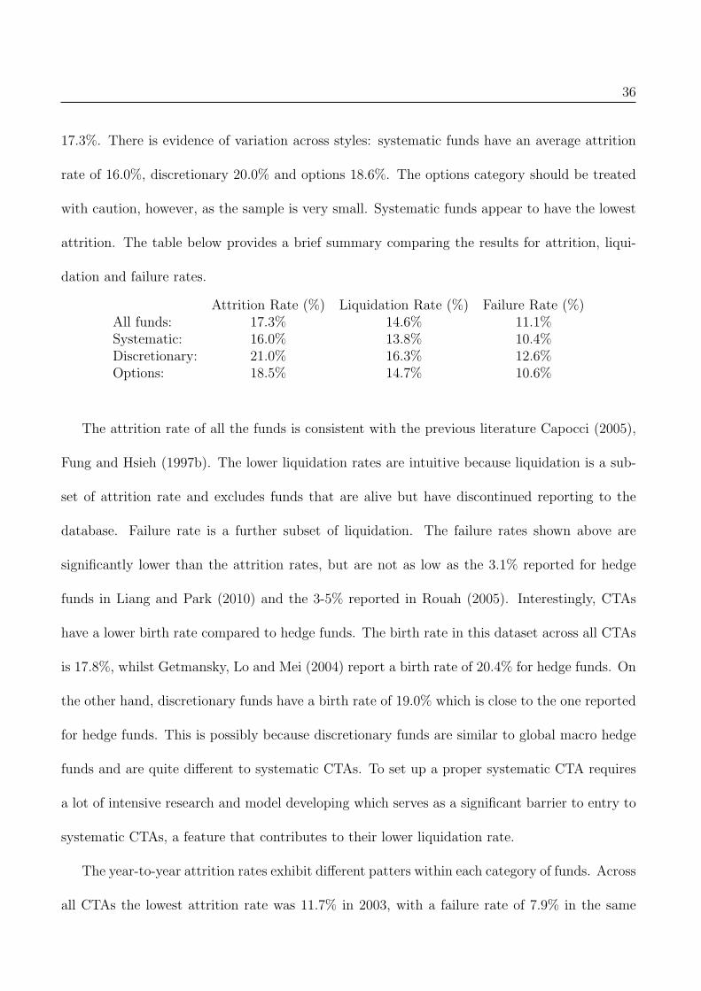
17.3%. There is evidence of variation across styles: systematic funds have an average attrition

rate of 16.0%, discretionary 20.0% and options 18.6%. The options category should be treated

with caution, however, as the sample is very small. Systematic funds appear to have the lowest

attrition. The table below provides a brief summary comparing the results for attrition, liqui-

dation and failure rates.

Attrition Rate (%) Liquidation Rate (%) Failure Rate (%)All funds: 17.3% 14.6% 11.1%Systematic: 16.0% 13.8% 10.4%Discretionary: 21.0% 16.3% 12.6%Options: 18.5% 14.7% 10.6%

The attrition rate of all the funds is consistent with the previous literature Capocci (2005),

Fung and Hsieh (1997b). The lower liquidation rates are intuitive because liquidation is a sub-

set of attrition rate and excludes funds that are alive but have discontinued reporting to the

database. Failure rate is a further subset of liquidation. The failure rates shown above are

significantly lower than the attrition rates, but are not as low as the 3.1% reported for hedge

funds in Liang and Park (2010) and the 3-5% reported in Rouah (2005). Interestingly, CTAs

have a lower birth rate compared to hedge funds. The birth rate in this dataset across all CTAs

is 17.8%, whilst Getmansky, Lo and Mei (2004) report a birth rate of 20.4% for hedge funds. On

the other hand, discretionary funds have a birth rate of 19.0% which is close to the one reported

for hedge funds. This is possibly because discretionary funds are similar to global macro hedge

funds and are quite different to systematic CTAs. To set up a proper systematic CTA requires

a lot of intensive research and model developing which serves as a significant barrier to entry to

systematic CTAs, a feature that contributes to their lower liquidation rate.

The year-to-year attrition rates exhibit different patters within each category of funds. Across

all CTAs the lowest attrition rate was 11.7% in 2003, with a failure rate of 7.9% in the same

37

year. There is considerable variation in the attrition across the years, however. Attrition and

failure rates start to decline at the beginning of 2000 until they rise again to an unprecedented

levels (24.3%) in 2009. Discretionary CTAs have considerably larger attrition and failure rates,

with levels climbing to 30.4% for attrition and 12.2% failure in 2009. This is much higher than

the rates across systematic funds where both attrition and failure rates are fairly stable across

the years with the highest rates, in 2009, of 21.4% and 8.3% respectively. Of note is that, con-

trary to the findings of Getmansky, Lo and Mei (2004) for hedge funds, the attrition and failure

rates are lowest for systematic funds from 2000 to 2003. This period represents the bursting of

the technology bubble, when many hedge funds experienced bad performance. CTAs have been

documented by several studies to have performed particularly well during market downturns,

hence the decline in their failure rates Fung and Hsieh (1997b), Edwards and Caglayan (2001).

Although the data shows relatively high attrition rates for CTAs, these estimates are inflated

by the number of very small funds in the database. As shown in Figure 1.1, whereas 80% of

CTA funds have assets below US$20 million, most of the assets of the CTA industry are man-

aged by a very small number of funds. Table 1.5 shows attrition, liquidation and failure rates

after excluding all funds with assets below US$1 million, US$10 million, US$20 million. As

smaller funds are excluded, attrition, liquidation and failure rates drop, to the extent that, for

systematic CTAs in particular, the failure rate approaches the 3% figure reported in Liang and

Park (2010) for hedge funds. Yet this study used more extensive filters and included a larger

number of failures than in Liang and Park’s (2010) study. Excluding funds with assets less than

US$20 million reduces the attrition rate to less than 10% with an even lower rate for systematic

CTAs. Given that most hedge fund studies exclude funds with less than two years of data,

which would exclude a lot of funds with small AUM, it is not surprising that previous research

38

on hedge funds documented low attrition rates. Capocci (2005) included all the CTAs in his

attrition analysis, hence a large attrition rate. It is likely that funds with assets below US$1

million are traders trading their own capital and do not constitute proper funds, yet the large

number of these in the database tends to inflate the attrition rate. The results of this analysis

suggest that the attrition of CTAs is not as high as previously thought: if small funds are ex-

cluded and, in particular, if funds with assets below US$1 million are excluded, the attrition rate

drops to 11.7%. Liquidation and failure rates are even lower, with a failure rate approaching

3.4% for systematic CTAs, consistent with the practitioners’ view as presented in Derman (2006).

Non-parametric Approach: The Kaplan-Meier Analysis of CTA Sur-

vival

This study begins its empirical analysis by measuring median survival times of CTAs for the

period 1994-2009 using the Kaplan-Meier non-parametric approach. Such analysis can help

prospective investors to select funds that are more likely to survive a long time and thus avoid

liquidation. Panel A of Table 1.6 reports median survival times in months for the unfiltered

database across the three main CTA categories: systematic, discretionary and options, as well

as for three definitions of exit: all funds in the graveyard database, liquidated funds and failed

funds only. Panel B shows the same results but for data that has been filtered to exclude funds

than never reached US$5 million assets under management. This is a very basic filter that at-

tempts to remove the large number of very small CTAs, a problem that was discussed in section

4.1. The table also shows the median survival times for large and small funds in each category

and the respective p-value of the Log Rank test of equality between the two groups.

39

The results of Table 1.6 highlight an important difference between exit type; compared to

the results for other exits, median survival is longest for failed funds. In fact, median survival

also increases for liquidated funds, compared to using the entire graveyard, and further increases

for failed funds. All exits comprises liquidated funds, merged funds, fraud, not reporting funds

and funds that self-selected. Self-selected funds are defined as alive funds that no longer wish to

report as they are closed to new investors. Not reporting funds are funds that are also alive but

had to stop reporting for other reasons than capacity. For example, such funds may have stopped

reporting because they now manage their own assets only, have not achieved NFA registration,

are exempt, or other reasons not related to capacity. These funds, however, comprise only a

tiny fraction of the total funds, namely just 60. Similarly, unlike hedge fund databases, the

number of the self-selected funds is rather small, just 4% compared to 11% in Liang and Park

(2010) and 10.7% in Fung et al. (2008), possibly because CTAs are unlikely to be as affected by

capacity constraints as the other hedge fund strategies.11 This study also finds a few fraudulent

funds from various website filings. Table 1.6 Panel A shows that funds in the group “All exits”

have a median survival of 4.17 years (50 months), a result similar to the 4.42 years found in

Gregoriou et al. (2005), who used the entire graveyard in their analysis without applying any

filters. For liquidated funds, median survival drops to 4.75 years across all funds and to 5.75

years for all failed funds. This suggests that CTAs can experience other types of exit besides

failure and liquidation. Baba and Goko (2009) show different survival curves for different exit

types of hedge funds which underlines the importance of sorting graveyard into various exits.

Panel C gives an insight into these other types of exit and their effect on median survival times.

Fraudulent funds have the shortest median survival of 2.33 years. Also, funds that are still alive

but stop reporting due to capacity constraints or other reasons have a short median survival of 3

1199 out of 2446 funds are self selected.

40

years, which has a downward impact on the median survival of all exits compared to liquidated

funds only. This demonstrates that funds close fairly quickly once they reach enough assets.

The results are further confirmed in Figure 1.5 which shows survival curves by graveyard status

together with corresponding smoothed hazard curves. Although Figure 1.5 does not include

failed funds, since they form part of the liquidated funds, it clearly demonstrates that survival

and hazard curves differ substantially across different exit types, with fraudulent funds having

the lowest survival curve, a result that is consistent with Brown et al. (2009) who found that

funds with high operational risks at the extreme have a half-life of less than 3.5 years.

Table 1.6 also indicates that filtering the database for very small funds that comprise a large

share of the total number of funds has an effect on funds’ half-life. The median survival across

all exits is larger in Panel B than in Panel A: the median survival for all funds and all exit types

increases to 5.7 years, to 6.4 years for all liquidated funds and to 8.9 years for all failed funds.

Table 1.6 also reports on how survival time relates to strategy variation. Systematic funds have

the longest survival compared to discretionary funds and options funds. This is invariant to the

database used or exit type. In particular, the median survival of failed systematic funds that are

above US$5 million is 9.5 years. For discretionary funds the median survival is 6.8 years. The

superiority of systematic funds is invariant to whether the entire or the filtered database is used

and persists across all exit types, liquidated and failed funds.

There are also significant differences between large and small funds. Large and small CTAs

are defined as those with mean assets in the period 1994-2009 that are above and below the mean

assets of all CTAs in the same strategy. Across all strategies, choosing a larger fund increases

the survival of a CTA. For example, the median survival of systematic liquidated funds above

US$5 million is 221 months for large funds and only 72 months for small funds. The difference

41

is statistically significant at the 1% significance level. The difference between large and small

funds is statistically significant across all strategies and all funds apart from options funds in

the failed and liquidated category (Panel B). This is consistent with the findings in Table 1.5

that shows the attrition of larger funds dropping. Larger asset base is therefore associated with

longevity.

Table 1.7 compares median survival across various strategies and two exit types, all exits

and failures only, for 892 CTAs that were filtered using a dynamic AUM filter as proposed in

Avramov, Barras and Kosowski (2010). The authors argue that few institutional investors wish

to represent more than 10% of a fund’s assets under management. According to the practitioner

side, reported in L’habitant (2006), a typical number of funds held by a fund of funds is about

40. Therefore the dynamic AUM cutoff filter is equal to the minimum fund size such that a

“typical” fund of funds does not breach the 10%-threshold.12 Applying this filter, the resulting

cutoff rises from $13 million in 1994 to $54 million in 2009. In comparison to Table 1.6, with a

dynamic AUM filter applied, the median survival increases, reinforcing the contention that larger

assets are associated with longevity. The p-value for the Log-Rank test is still significant across

all funds and all exit types, indicating that there are still significant differences between large

and small funds, despite the fact that the funds have been filtered by asset size. The median

survival of all funds for all exits increased to 77 months (6.4 years) and to 130 months (10.8

years) for failed funds. Systematic funds again have the longest half-life across both exit types:

144 months for failed funds and 105 months for all exits, indicating that this is the strategy with

the longest longevity. This result is further demonstrated in Figure 1.6 which shows a plot of

survival and hazard curves for systematic and discretionary funds. The result also supports the

12The typical fund of funds is defined as a fund with an average AUM as measured by the fund of funds AUMin the database which on average invests into 50 CTAs.

42

earlier finding of Table 1.5 where systematic CTAs were shown to have the lowest attrition and

failure rates. This points to differences within different types of CTAs and supports the earlier

argument that, contrary to previous studies that grouped all CTAs, it is better to analyze these

funds by separating systematic and discretionary funds.

There are some variations with sub-strategies. Systematic trend-followers, led by short-term

trend-followers have the highest median survival; a result further supported in Figure 1.7 which

shows survival and hazard curves across different sub-strategies of CTAs for 892 failed funds.

This result is consistent with Capocci (2005) and Gregoriou et al. (2005) who argue that there

are significant difference across CTA styles. Panel B demonstrates that an investor randomly

selecting a newly launching systematic short-term trend-following fund can expect the fund to

survive 12.7 years before liquidation and failure. Choosing a large fund in this category will

further increase the survival to 14.3 years (172 months), whilst a small fund will survive 9.5

years. The difference is statistically and economically significant at 1%. On the other hand, an

investor investing into a newly launching discretionary fundamental fund can expect the fund

to survive for 7.8 years (93 months) before failing. These results are in sharp contrast to the

median survival times reported in Gregoriou et al. (2005). There the authors report survival

times that are significantly lower than in this study, with overall survival times of just 4.42 years.

This is because their study used the entire graveyard as their definition of failure and therefore

their results are only directly comparable to the results of Panel A in Table 1.6. Neither does

their study filter out small funds from the sample which could further influence the results. Fur-

thermore, unlike this study, the authors follow the strategy classification of BarclayHedge and

therefore obtain very different results across CTA classifications. Accordingly, they find that

systematic funds have the lowest median survival of only 3.33 years, whereas this study finds

43

that systematic funds have the highest survival of 4.42 years,13 even when using the unfiltered

database and treating all exits as failures. The median survival time changes significantly with

dynamic AUM filtering and using only failed funds, raising the median survival of systematic

funds to 12 years (144 months). In fact, on this approach the entire ranking is reversed. In

contrast to the approach of Gregoriou et al., Diz (1999b) uses Barclay Trading Group for the

period 1975 to 1995 and finds that systematic traders have a greater probability of survival than

discretionary. These results highlight the importance of different types of exits that need to be

carefully accounted for together with the need for clear strategy definition that is yet to be con-

clusively established in the CTA space. Furthermore, they show that using the entire graveyard

as definition of failure can impart a significant downward bias on medial survival. Standard

deviation has no impact on media survival of CTAs which resonates with the results of Liang

and Park (2010) for hedge funds.

Finally, Table 1.8 reports results of several Log-Rank tests for equality of survival functions

for each sample stratified by the covariates of interest. This table is comparable to the one in

Gregoriou et al. (2005) but is applied to the sample with a dynamic AUM filter and with failure

only as the exit type. Similarly to Gregoriou et al. (2005) the results indicate that CTAs with

above average mean return (≥ 0.95%) survive longer as well as those with above average assets

under management (≥ $103 million). Gregoriou et al. (2005), however, report lower survival

times of 5.33 years and 6.16 years respectively in comparison to 14.67 years and 12.17 years for

filtered failed funds in this study. Table 1.8 also reports that while funds with higher manage-

ment fees and incentive fees survive longer, the difference in survival time is only statistically

significant for performance fees. This is in contrast to Gregoriou et al. (2005) who find that

management fees positively impact survival times. Similarly to Gregoriou et al. (2005), however,

1353 months, from Panel A in Table VII

44

Table 1.8 reports no difference in survival when the sample is grouped by the standard deviation.

Minimum purchase also has a very weak effect on survival times. The results indicate that the

monthly return, average funds managed and performance fees have an important implication on

the survival.

Cox Proportional Hazards Model

A Survival Analysis to Predict Attrition

In the remainder of the analysis the sample consisted of funds that were selected with a dynamic

AUM filter - thus reducing the sample to 892 CTAs. Table 1.9 presents the results of fitting the

Cox proportional hazards model of Gregoriou et al. (2005) and follows a conventional classifica-

tion that defines failure as all exits to the graveyard. The first column is a parameter estimate

and the second reports the associated hazard ratio, which is eβ for the covariate. Hazard ratio

provides an easier interpretation of the level of a covariate’s influence. For binary variables with

values of 1 or 0, the hazard ratio can be interpreted as the ratio of hazard for those with a value

of 1 to the estimated hazard for those with a value of 0, after controlling for other covariates.

For quantitative variables, the hazard ratio estimate needs to subtract 1 and multiply by 100

which gives a percentage change in the hazard for each unit increase in the covariate, control-

ling for other variables. According to Allison (1995) a simple interpretation of the estimated

hazard ratio is that a hazard ratio greater than one implies a negative effect of the covariate on

survival, while a hazard ratio less than one indicates a protective effect of the covariate. The

corresponding p-value reports the p-value for the Wald test of the null hypothesis that each

45

coefficient is equal to zero. The results indicate that only three variables have a significant effect

on survival: mean monthly return over the entire life of the fund, average millions managed

and management fees. It is found that higher average monthly returns as well as assets under

management are protective whereas higher management fees are not. The results closely mirror

the findings of Gregoriou et al. (2005) even though the sample in this study was filtered by asset

size. Specifically, the hazard ratio of the mean return is 0.838, indicating that an increase in

the monthly return of 1% leads to 16.2% reduction in the likelihood of failure. The protective

effect of the AUM is marginal. However, every percentage point increase in the management

fee increases the likelihood of failure by 15.2%. The goodness of fit provided by the Likelihood

ratio test and the Global Wald test, both are significant, and lends support to the accuracy of

the functional form of the model.

For comparison, Table 1.10 reports the results of the Liang and Park (2010) LP model, with

failure defined as exit to the graveyard. Compared to the LP model, where all risk measures

are significant when they are the only explanatory variables, Panel A shows that only standard

deviation and expected shortfall are significant risk measures. When other explanatory vari-

ables are added to the model, Panel B, standard deviation loses its significance but value at

risk becomes significant at 10%. This supports the earlier results of Table 1.9 that standard

deviation is not a useful measure of CTA survival. The hazard ratios of the VAR and ES are

below one, which is not intuitive since it implies that higher risk funds have lower hazards. This

strengthens the argument of Rouah (2005) that the effect of the covariates becomes blurred

when all the graveyard funds are regarded as failures. With regard to the impact of the other

variables, Table 1.10 shows that only standard deviation of the AUM, leverage, HWM and a

dummy variable for discretionary style are significant at the 1% significance level. Interestingly,

46

the hazard ratio of leverage is protective. Baba and Goko (2009) conducted a Tobit analysis

with mean leverage as the dependent variable. They found that funds with high mean leverage

also tended to have a larger AUM, a high water mark and a longer redemption period. These

factors alone can lower the hazard ratios. The hazard ratio of high water mark in Table 1.10

is above one, indicating that CTAs with high water mark have increased risk of failure by as

much as 60%, which is contrary to the results in Liang and Park (2010) who find HWM to be

protective. Rouah (2005) also finds that HWM increases the risk of failure. The effect of high

watermark on hedge fund survival remains unclear with different authors presenting different

results. Rouah (2005), Ng (2008) and Lee (2010) all used the HFR database to study hedge

fund survival and each found that HWM tended to increase failure, whereas Liang and Park

(2010) and Baba and Goko (2010) analysed hedge fund survival using the TASS database and

found that HWM is protective. The authors argue that the HWM facilitates more stable fund

management as well as serves a signal quality for good managers. Liang and Park (2010) also

cite Aragon and Qian (2005) who argue that HWM lowers existing investors’ marginal cost of

staying in the fund following its poor performance and hence allows fund managers to avoid

liquidation by keeping its investors. Liang (2000), Brown, Goetzmann and Ibbotson (1999) and

Rouah (2005), on the other hand, suggest that once the fund incurs large losses it is difficult

for the manager to recuperate them and attain its high water mark and that this increases the

incentive to liquidate. Gregoriou et al. (2005) do not include HWM in their model therefore it

is impossible to obtain a direct comparison for this study. It is more likely, however, that the

effect of HWM on CTA survival is negative, given the significance and the size of the hazard

ratio.

Table 1.10 also shows that there are some style effects: discretionary funds have a higher

47

hazard rate relative to systematic funds. Investing into a discretionary fund entails a hazard

rate 37% higher than in systematic CTAs. The explanatory power of the mean return and mean

AUM in the last year of a fund’s life is weak, indicating the need for separating exit types. In

addition to reporting the significance of the hazard ratios, Table 1.10 also reports “Rho”, which

is a slope estimate for each variable of the scaled Schoenfeld (1982) residuals against time. Un-

der the null hypothesis of proportional hazards, the curve is expected to have a zero slope, thus

rejection of the null hypothesis indicates a deviation from the proportional-hazards assumption.

The Global Ph Wald test is a Wald statistic that tests whether all the covariates jointly satisfy

the proportional hazard assumption, i.e. model specification. Apart from the model with ES

as the risk measure, the global Wald test shows that the proportional hazards assumption is

rejected as a whole at the 1% significance level, whilst only one variable, standard deviation of

AUM, violates it.

A Survival Analysis to Predict Liquidation

The graveyard contains different types of exits, as reported in Table 1.6: liquidated funds, funds

that are alive but stopped reporting due to capacity constraints or simply self-selected funds.

Rouah (2005) argues that only liquidated funds should be used in the survival analysis in order

to avoid blurring the effect of predictor variables. Table 1.11 reports the results of fitting the

LP Cox proportional hazards model on liquidated funds only, that is the number of failed funds

reduces to 441 from 529 and other types of exit are treated as censored. This model shows

a marginal improvement in that both mean return and mean AUM become significant at 1%,

however neither satisfy the proportional hazards assumption. The effect of risk measures in the

48

univariate and multivariate models remains unchanged. This is similar to the results of Liang

and Park (2010) who find that a model with liquidated funds produced misleading estimates.

In what follows, therefore, the analysis concentrates only on failed funds identified with perfor-

mance and AUM filters as discussed previously.

A Survival Analysis to Predict Failure

As discussed above, using liquidated funds is still not very informative in defining failure since

many funds liquidate for reasons other than bad performance, e.g. merging with another fund.

The remainder of the analysis, therefore, concentrates on the failed funds only. Table 1.12 shows

several model specifications for failed funds with fixed covariates only. For comparison purposes,

specification (i) includes the same variables as in the Gregoriou et al. (2005) model but applied

to failed funds only. In contrast to Table 1.6, where all exits were treated as failure, Table 1.12

shows that the standard deviation over the entire life of the fund is now significant at 1% with

a hazard ratio above one. Management fee is still significant and increases the likelihood of

failure. The second specification adds skewness, kurtosis, winning ratio,14 standard deviation of

AUM over entire life of the fund, whether the fund has a hurdle rate, employs leverage, HWM

and dummy variables for investment style. Skewness and kurtosis are significant at 5% and 10%

respectively as well as the volatility of assets, leverage and the dummy for discretionary style.15

The effect of skewness is protective: a unit increase in the skewness decreases the hazard rate

of the fund by 14%. One would expect the survival to be positively related to the first and

14The number of months with a positive return to the total number months.15The dummy variable for systematic style was removed to avoid perfect multicollinearity in the estimation

process. The coefficient of the other two strategy dummies represents the incremental change in hazard ascompared to the default case.

49

third moments and negatively to the second and fourth moments. Contrary to this expectation,

however, the coefficient on kurtosis is negative indicating that it aids in survival. The effect

is, however, marginal and the covariate is not significant in specification (iii). The effect of the

winning ratio is to decrease the hazard rate of the fund whilst management fee increases the

hazard rate. Similar to previous results, leverage is protective and discretionary funds are 57%

more likely to fail than systematic ones. The hurdle rate is insignificant and is not included in

the remaining specifications due to its incomplete data.

Specification (iii) further adds maximum drawdown over the entire life of the fund. Similar to

the finding of Diz (1999b), this variable is highly significant and increases the hazard rate by 5%

for every percentage increase in the drawdown. The hazard ratio of the winning ratio decreases

to 0.08 at 1% significance level. The interpretation needs care, however, as the win ratio is the

number of positive returns over the total number of returns and is therefore between 0 and 1,

hence even a slight increase in this number can dramatically increase the estimated survival.

In the final specification in Table 1.12 maximum drawdown is replaced by maximum drawdown

relative to standard deviation. It shows that once maximum drawdown reaches three times an-

nualized standard deviation the hazard rate increases by as much as 213%. If the drawdown is

within two standard deviations, the effect is protective, but above two standard deviations the

fund is at risk of failure. The effect of HWM is significant in this model - funds with high water

mark provision have an increased risk of failure by as much as 51% relative to funds without

it. The effect of discretionary funds is unchanged, but the hazard ratio of the options funds be-

comes significant at 5% and demonstrates an increased hazard rate of the options funds relative

to systematic ones.

Table 1.13 compares the five risk measures in terms of predicting the “real failure” of CTAs by

50

using Liang and Park’s (2010) model. Standard deviation remains an insignificant risk measure

but semideviation, ES and TR each become significant. In particular, the effect of semideviation

is to increase the hazard rate by 5%, whilst TR increases the hazard rate by 2%. The effect of

ES remains unclear, however, since the hazard ratio is marginally below one. Mean return is

found to be a highly significant covariate at the 1% level with a hazard ratio of 0.84, implying

that high return funds have a lower hazard rate of failure. The fund size, as represented by the

mean assets under management over the entire life of the fund, is significant at 1%, however the

effect on survival is negligible. In addition this variable has a significant Rho, indicating that

it violates the proportionality assumption. In fact both mean AUM and standard deviation of

AUM violate the proportionality assumption. The previous studies of Ng (2008) and Lee (2010)

included fund size as the natural logarithm of the fund’s assets under management at the last

month. The authors argue that the effect of the fund size on the duration is non-linear. One

way to test this is to use the Martingale residuals to test for the best functional form of the

covariate. The goal is to determine the best functional form that will result in an approximately

straight curve of the martingale residuals against the covariate. In unreported tests we plot

mean AUM against martingale residuals and log AUM against martingale residuals. The log

transformation of the recent AUM yields a linear plot against martingale residuals, indicating a

better fit. Given this result, we use natural logarithm of fund’s assets under management at the

last month rather than just assets under management in the survival model.

Table 1.14 extends Liang and Park’s (2010) model by including a larger set of covariates

than were previously tested in the base model as well as replacing mean AUM with the log

of the last month AUM. In addition, Drawdown/STD is added as another risk measure. The

most significant covariates, at 1% level, are mean return, fund size represented by the log of last

51

month AUM, standard deviation of the AUM, a dummy for discretionary strategy and leverage.

The protective effect of the mean return relative to previous models increases with an increase

in mean return over the entire life of the fund resulting in a decrease in the hazard rate of 43%.

The effect of fund size is also much stronger now with one unit increase in size reducing the

hazard rate by 15%. The effect of standard deviation of AUM is negligible and both variables

still show the rejection of the proportionality assumption with significant Rho. The way to cir-

cumvent this issue is by introducing these variables as time varying. Table 1.15 introduces AUM

as a time-varying variable. We also introduce another variable, asset flow, Flow(t). Following

Agarwal, Daniel and Naik (2009) monthly flow is defined as:

DollarF lowi,m = AUMi,m − AUMi,m−1 (1 +Returni,m) (24)

which is then scaled by the previous month’s assets under management as in Sirri and Tuffano

(1998) to obtain:

Flowi,m =DollarF lowi,m

AUMi,m−1

(25)

Baba and Goko (2009) are the first to include a flow variable in the survival analysis which

they justify by the return-chasing behaviour of investors, where investors flock to funds with

good recent performance and withdraw funds from poorly performing funds (Chan et al. 2006).

Agarwal et al. (2009) also document that money flows chase good recent performance and find

that this relationship is in fact convex. However, they also find that larger funds with greater

inflows are associated with poorer future performance underlining that hedge funds face dimin-

ishing returns to scale. Baba and Goko (2009) find the effect of Flow to be protective, i.e. recent

inflows contribute to lower liquidation probabilities. Table 1.15 shows that whilst the effect of

52

time-varying AUM is significant, the effect on survival is marginal whereas the protective effect

of Flow is significant at 1% and is indeed much stronger than documented in Baba and Goko

(2009), with a hazard ratio of 0.12. The effect of other variables seems to be unchanged: mean

return, skewness, winning ratio, management fee and leverage all remain significant. HWM is

no longer significant, whilst the incentive fee and minimum investment also remain insignificant.

With the inclusion of time-varying AUM and Flow, SEM, ES and TR remain significant and

VAR gains significance at 10%. The Likelihood ratio increases to 289.10 compared to 199.02 in

Table 1.14 indicating an overall improvement in the model. Finally Table 1.16 adds ten dummy

variables of which the eleven’s strategy, Fundamental and Technical, was removed to avoid per-

fect multicollinearity in the estimation process.16 The coefficient of the other ten strategies

represent the incremental change in the hazard as compared to the default case, the fundamen-

tal and technical strategy. For example, the hazard ratio of short-term trend followers is 0.41,

meaning it is 59% less likely to fail than discretionary CTAs employing a fundamental and tech-

nical approach. The results indicate that only a few strategies are significant at the 1% level:

short-term and medium-term trend followers. The coefficient on discretionary CTAs with a fun-

damental approach is significant in the models with TR and Drawdown/STD as risk measures,

and systematic counter trend funds are 150% more likely fail than the default strategy. This is

easy to understand since it is a rather difficult strategy to implement, as evidenced by the small

number of counter trend funds.

Of particular interest in the above is the negative relationship between management fee and

survival. The results across all tables demonstrate that, on average, an increase in management

fee leads to an approximately 15% increase in the hazard rate. This is similar to the result in

16Table 1.16 presents only the results for standard deviation, TR and drawdown/STD. The results of the modelwith the remaining risk measures are omitted to save space.

53

Gregoriou et al. (2005) but the effect is stronger for failed funds only. Baba and Goko (2009),

however, find that the effect is reversed for hedge funds where management fee is protective

whilst incentive fee is not. HWM becomes insignificant when time-varying AUM and Flow are

added to the model.

Robustness Checks

In unreported results we test to see if our results are affected by changes in the confidence level

of the risk measures or the use of different estimation models.

Changing the confidence level of the risk measures

The results above are further examined to determine if they are affected by the confidence level

chosen to calculate VAR, ES and TR. Current results present a 95% confidence level. The re-

sults at the 99% confidence level are not much different to the results presented earlier. Standard

deviation still appears to be insignificant in predicting real failure whilst SEM, ES and TR are

significant at the 5% level.

The Probit Model

Malkiel and Saha (2005) and Brown et al. (2001) use a probit model to estimate the effect of

variables on hedge fund survival. Using a probit model on the 817 funds for failure and attrition

shows that results are not dissimilar to the Cox (1972) model. Standard deviation is still less

efficient at predicting survival than other risk measures.

54

Conclusion

This chapter has analyzed the factors affecting CTA survival. It included a wide range of vari-

ables with particular emphasis on various downside risk measures as well as AUM and capital

flows. In addition, it has offered an improvement in methodology when compared to previous

studies on CTA survival. In contrast to previous survival analyses that incorporated only fixed

covariates, this study included time varying covariates which allowed to evaluate their impact at

each instant of a fund’s lifetime rather than during the entire lifetime or the last 12 months. This

study also adopted a novel CTA strategy classification that allowed for interesting comparisons

between discretionary and systematic CTAs. Finally, it has taken into account the different exit

types that CTAs can experience. It used a combination of various filters and hand-collected

information to determine exit types. Further, an updated filtering methodology was proposed

to screen for failed funds among CTAs. Based on this extensive data collection, the attrition

rate and factors affecting CTA survival are investigated.

The main results demonstrate that the entire graveyard is a poor measure of CTA failure

and it is therefore important to account for different exit types. Whilst attrition of CTAs is as

high as 17.8%, similar to the rate for all hedge funds, the average percentage of liquidated funds

is lower at 14.6%. However, once the real failures among the liquidated funds are distinguished,

the rate drops to 11.1% suggesting that there are many discretionary liquidations that are not

damaging to investors. As such this study develops filters to discriminate between failed funds.

It also finds that the CTA database contains a large number of small funds with assets that are

less than US$20 million. Institutional investors are unlikely to invest into such small funds and

if they are removed from the sample the real failure rate drops to 3.9%, which is comparable to

the failure rate reported for hedge funds. The failure rate for CTAs is therefore not as high as

55

previously thought. Systematic CTAs are also found to have a lower failure rate than discre-

tionary ones, 3.4% vs. 5.8%. This study also demonstrates that the attrition rate during the

2008 financial crisis climbed to an unprecedented level.

Further, the median survival time of large failed funds is found to be 10.8 years, which is

higher than the previously reported median survival of 4.42 years in Gregoriou et al. (2005) and

of 2 years reported in Brown et al. (2001). Spurgin (1999) has used the MAR CTA database

over a shorter period and reports a survival time of approximately 5 years. Our results show

that an average systematic CTA has a median survival of 12 years compared to 8.33 years for

a failed discretionary fund. Assets under management have an effect on survival as well, with

larger funds having significantly higher median survival times when compared to smaller funds.

Using Cox’s (1972) model with time-varying covariates the results show that standard devi-

ation is not a good risk measure in terms of predicting CTA failure. Measures such as SEM and

TR as well as maximum drawdown are better able to account for non-normality of CTA returns.

Apart from variables such as performance and assets under management, asset flows into the

funds have a positive effect on CTA survival. Funds that experience significant asset outflows

have a higher chance of liquidation. Contrary to the findings of Liang and Park (2010) for hedge

funds, the presence of a high water mark has a negative effect on CTA survival. Management

fees increase the probability of failure whilst leverage has a protective effect. The effect of lever-

age could possibly be explained by the findings of Brown et al. (2009) as further discussed in

Brown, Goetzmann, Liang and Schwarz (forthcoming), who find that funds with higher opera-

tional risks are less able to raise leverage since prime brokers and lenders are less willing to lend

to funds that they perceive as risky. Conversely, funds that are more able to borrow may have

less operational risk and thus lower liquidation probabilities. The results also show that funds

56

with lower skewness, lower winning ratio and higher maximum drawdown have higher failure

rates. Finally, there are important differences across CTA styles, with systematic CTAs and in

particular systematic trend-followers experiencing lower hazard rates than any other strategy

and these should therefore be favoured by investors.

57

Appendix

SYSTEMATIC - funds that employ purely systematic approach to trading, utilizing computer

models that are mainly based on technical analysis of the market data and fundamental eco-

nomic data. Trading can be diversified across many markets, including foreign exchange,

interest rates, commodity, bond and equity markets. Manager intervention is limited. The

core of systematic trading lies in strict management of volatility. “Diversified program is a

diversified portfolio of more than 120 international futures and forwards markets employing

a computer based system. The system has been developed based on the basis of a sophisti-

cated statistical analysis of past price movements and seeks to profit from the tendency of

the markets to trend.” Winton Capital Management, Ltd.

Trend-following - by far the most represented strategy among systematic funds. This is

a strategy that tries to take advantage of price movements in a systematic way and aims

to work on the market trend, taking benefit from both up markets and down markets.

“Bluetrend fund is a systematic, trend-following black box fund, which trades on a 24 hour

cycle and seeks to successfully identify trends.” BlueCrest Capital Mgmt, LLP.

Trend-following - Short-term - Systematic trend-follower with a short-term time

frame of anything from intra-day trading up to one week.

Trend-following - Medium-term - Systematic trend-follower with a medium-term

time frame of anything from one week to 30 days. “Rotella Sirius Fund, LLC utilizes a

multi-model approach targeting medium-term and long-term trends in global commodity,

interest rate, currency and equity index markets. Sirius’s average holding period is 25-50

days.”

58

Trend-following - Long-term - Systematic trend-follower with a long-term time

frame from one month to several months.

Pattern Recognition - Systematic trading that bases its approach on statistical pattern

recognition in a variety of markets, utilizing a particular field of computer science concerned

with recognizing patterns. “The trader exploits non-random price behaviour by quantitative

analysis of price patterns. Its approach is entirely systematic. The systems are applied

to more than 100 different product-market-combinations. Advanced correlation analysis

safeguards portfolio balance.” Transtrend.

Spread/Relative Value - a systematic approach to arbitrage and relative value trading.

Relative Value Arbitrage is a market neutral strategy that seeks to exploit pricing in-

efficiencies between related securities and markets, including equities, options, debt and

futures. Managers tend to use mathematical models and technical analysis.

Counter Trend - systematic trading that takes advantage of price movements by adopt-

ing a contrarian approach to the trends. “The Financials Program employs a quantita-

tive, primarily contrarian, short-term strategy. RGNCM’S method captures changes in the

psychology of market participants and has been particularly successful during volatile and

declining equity and fixed income markets” R.G. Niederhoffer Capital Management.

DISCRETIONARY - whereas systematic trading uses a fixed set of rules to determine trade

entries and direction, the discretionary trader is not bound by any rules. In essence the

trader uses his own judgement and evaluation of the market indicators, fundamental in-

formation, etc. to determine the value of the indicator and decides the point of entry, size

of investment and level of risk taking.

59

Fundamental - discretionary trading that focuses on the analysis of fundamentals to inform

investment decisions. Programs may focus on one market only or diversified markets.

“Albion utilizes a fundamental based discretionary approach to trade the major currencies.”

Albion Currency Advisors, Ltd

Technical - discretionary trading that uses technical analysis, such as charts and price

patterns, with most trading executed by the manager. Some funds may utilize computer

based systems to look for price patterns but ultimately all the trading is executed by the

manager.

Fundamental and Technical - a mixture of fundamental and technical analyses with man-

ager discretion.

Discretionary Spread/RV - exploiting arbitrage opportunities with manager discretion.

OPTIONS STRATEGIES

Options Writing - programs that rely on selling or writing options.

Options Other - programs that utilize options trading other than selling. “Reflects the

performance of the Options Program - an intermediate term market neutral anti-trend

following approach combining 60% fundamental and 40% technical analysis to trade U.S.

fixed income and equity options” Analytic TSA Global Asset Mgmt, Inc.

60

All CTAs 2446

Systematic 1511Trend-Followers 1263

Short-Term 331Medium-Term 780Long-Term 152

Pattern Recognition 96Spread/Relative Value 128Counter Trend 24

Discretionary 747Fundamental & Technical 253Fundamental 136Technical 284Spread/Relative Value 74

Options 188Options Writing 113Options Other 75

61Tab

le1:

Summary

Statistics

Tab

le1.1show

sthenumber

ofob

servations(N

),meanvalues

ofsample

average,

standard

deviation,skew

nessandkurtosis

ofindividual

CTA

returns.

Thedatais

from

theBarclay

Hedge

database

forthesample

periodfrom

January

1994to

Decem

ber

2009.Thetable

also

show

sthepercentage

ofCTA

fundsthat

reject

theJarque-Bera(JB)test

ofnorm

ality

atthesignificance

of1%.TheJB

statistichas

χ2

distribution

.

Drop

No.

ofMeanreturn

Std.Dev.Skew

nessKurtosis

Min

return

Max

return

JB

test

ofReasons

Funds

(%)

(%)

(%)

(%)

Normality(%

)

Livefunds

696

1.19

5.36

0.31

2.86

-11.80

18.23

45.11

Graveyardfunds

1750

0.93

6.38

0.34

2.51

-13.01

18.78

40.57

Not

reportingfunds

265

1.93

5.99

0.41

2.23

-10.62

18.53

39.25

Liquidated

funds

1485

0.76

6.45

0.33

2.56

-13.45

18.83

40.81

Discretionary

352

1.52

5.06

0.49

2.64

-8.94

16.76

43.18

Failures

1133

0.50

6.91

0.25

2.54

-14.95

19.52

40.07

Allfunds

2446

1.01

6.09

0.33

2.61

-12.67

18.23

41.9

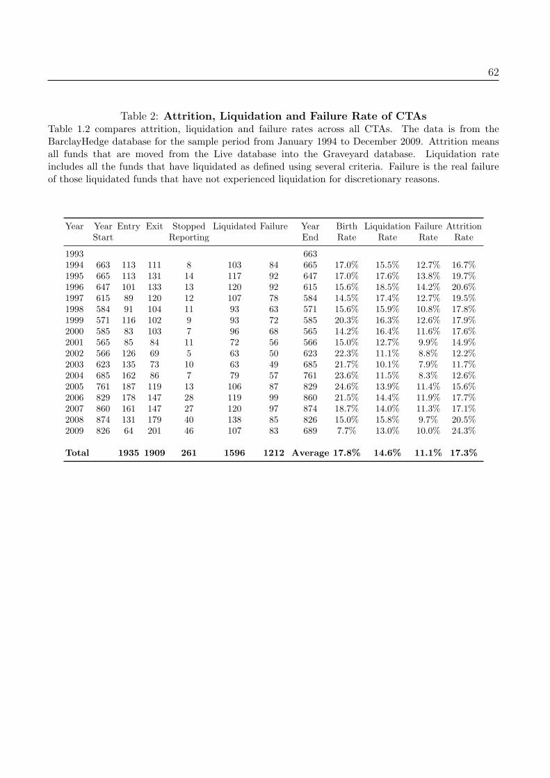
62

Table 2: Attrition, Liquidation and Failure Rate of CTAsTable 1.2 compares attrition, liquidation and failure rates across all CTAs. The data is from theBarclayHedge database for the sample period from January 1994 to December 2009. Attrition meansall funds that are moved from the Live database into the Graveyard database. Liquidation rateincludes all the funds that have liquidated as defined using several criteria. Failure is the real failureof those liquidated funds that have not experienced liquidation for discretionary reasons.

Year Year Entry Exit Stopped Liquidated Failure Year Birth Liquidation Failure AttritionStart Reporting End Rate Rate Rate Rate

1993 6631994 663 113 111 8 103 84 665 17.0% 15.5% 12.7% 16.7%1995 665 113 131 14 117 92 647 17.0% 17.6% 13.8% 19.7%1996 647 101 133 13 120 92 615 15.6% 18.5% 14.2% 20.6%1997 615 89 120 12 107 78 584 14.5% 17.4% 12.7% 19.5%1998 584 91 104 11 93 63 571 15.6% 15.9% 10.8% 17.8%1999 571 116 102 9 93 72 585 20.3% 16.3% 12.6% 17.9%2000 585 83 103 7 96 68 565 14.2% 16.4% 11.6% 17.6%2001 565 85 84 11 72 56 566 15.0% 12.7% 9.9% 14.9%2002 566 126 69 5 63 50 623 22.3% 11.1% 8.8% 12.2%2003 623 135 73 10 63 49 685 21.7% 10.1% 7.9% 11.7%2004 685 162 86 7 79 57 761 23.6% 11.5% 8.3% 12.6%2005 761 187 119 13 106 87 829 24.6% 13.9% 11.4% 15.6%2006 829 178 147 28 119 99 860 21.5% 14.4% 11.9% 17.7%2007 860 161 147 27 120 97 874 18.7% 14.0% 11.3% 17.1%2008 874 131 179 40 138 85 826 15.0% 15.8% 9.7% 20.5%2009 826 64 201 46 107 83 689 7.7% 13.0% 10.0% 24.3%

Total 1935 1909 261 1596 1212 Average 17.8% 14.6% 11.1% 17.3%

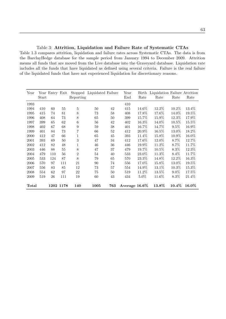
63

Table 3: Attrition, Liquidation and Failure Rate of Systematic CTAsTable 1.3 compares attrition, liquidation and failure rates across Systematic CTAs. The data is fromthe BarclayHedge database for the sample period from January 1994 to December 2009. Attritionmeans all funds that are moved from the Live database into the Graveyard database. Liquidation rateincludes all the funds that have liquidated as defined using several criteria. Failure is the real failureof the liquidated funds that have not experienced liquidation for discretionary reasons.

Year Year Entry Exit Stopped Liquidated Failure Year Birth Liquidation Failure AttritionStart Reporting End Rate Rate Rate Rate

1993 4101994 410 60 55 5 50 42 415 14.6% 12.2% 10.2% 13.4%1995 415 74 81 8 73 58 408 17.8% 17.6% 14.0% 19.5%1996 408 64 73 8 65 50 399 15.7% 15.9% 12.3% 17.9%1997 399 65 62 6 56 42 402 16.3% 14.0% 10.5% 15.5%1998 402 67 68 9 59 38 401 16.7% 14.7% 9.5% 16.9%1999 401 84 73 7 66 52 412 20.9% 16.5% 13.0% 18.2%2000 412 47 66 1 65 45 393 11.4% 15.8% 10.9% 16.0%2001 393 69 50 3 47 34 412 17.6% 12.0% 8.7% 12.7%2002 412 82 48 1 46 36 446 19.9% 11.2% 8.7% 11.7%2003 446 88 55 8 47 37 479 19.7% 10.5% 8.3% 12.3%2004 479 110 56 2 54 40 533 23.0% 11.3% 8.4% 11.7%2005 533 124 87 8 79 65 570 23.3% 14.8% 12.2% 16.3%2006 570 97 111 21 90 74 556 17.0% 15.8% 13.0% 19.5%2007 556 83 85 12 73 57 554 14.9% 13.1% 10.3% 15.3%2008 554 62 97 22 75 50 519 11.2% 13.5% 9.0% 17.5%2009 519 26 111 19 60 43 434 5.0% 11.6% 8.3% 21.4%

Total 1202 1178 140 1005 763 Average 16.6% 13.8% 10.4% 16.0%

64

Table 4: Attrition, Liquidation and Failure Rate of Discretionary CTAsTable 1.4 compares attrition, liquidation and failure rates across Discretionary CTAs. The data is fromthe BarclayHedge database for the sample period from January 1994 to December 2009. Attritionmeans all funds that are moved from the Live database into the Graveyard database. Liquidation rateincludes all the funds that have liquidated as defined using several criteria. Failure is the real failureof the liquidated funds that have not experienced liquidation for discretionary reasons.

Year Year Entry Exit Stopped Liquidated Failure Year Birth Liquidation Failure AttritionStart Reporting End Rate Rate Rate Rate

1993 2441994 244 49 54 3 51 40 239 20.1% 20.9% 16.4% 22.1%1995 239 37 49 6 43 34 227 15.5% 18.0% 14.2% 20.5%1996 227 31 55 4 51 38 203 13.7% 22.5% 16.7% 24.2%1997 203 20 53 4 48 34 170 9.9% 23.6% 16.7% 26.1%1998 170 20 33 2 31 24 157 11.8% 18.2% 14.1% 19.4%1999 157 26 29 2 27 20 154 16.6% 17.2% 12.7% 18.5%2000 154 25 34 5 29 21 145 16.2% 18.8% 13.6% 22.1%2001 145 9 31 7 23 20 123 6.2% 15.9% 13.8% 21.4%2002 123 39 19 4 15 12 143 31.7% 12.2% 9.8% 15.4%2003 143 34 12 1 11 8 165 23.8% 7.7% 5.6% 8.4%2004 165 40 25 4 21 16 180 24.2% 12.7% 9.7% 15.2%2005 180 41 30 5 25 21 191 22.8% 13.9% 11.7% 16.7%2006 191 66 27 5 22 21 230 34.6% 11.5% 11.0% 14.1%2007 230 60 52 14 38 33 238 26.1% 16.5% 14.3% 22.6%2008 238 49 50 11 38 20 237 20.6% 16.0% 8.4% 21.0%2009 237 25 72 24 35 29 190 10.5% 14.8% 12.2% 30.4%

Total 571 625 101 508 391 Average 19.0% 16.3% 12.6% 21.0%

65

Table 5: Attrition, Liquidation and Failure Rate Across Styles by AUMTable 1.5 compares attrition, liquidation and failure rates across CTA styles. The data is from theBarclayHedge database for the sample period from January 1994 to December 2009. Attrition meansall funds that are moved from the Live database into the Graveyard database. Liquidation rateincludes all the funds that have liquidated as defined using several criteria. Failure is the real failureof the liquidated funds that have not experienced liquidation for discretionary reasons.

CTA Style Birth Rate Attrition Rate Liquidation Rate Failure Rate

All fundsAll CTAs 17.8% 17.3% 14.6% 11.1%Discretionary 19.0% 19.9% 16.3% 12.6%Systematic 17.8% 16.0% 13.8% 10.4%

Excluding funds with AUM less than US$1 million.All CTAs 16.4% 14.1% 11.7% 8.6%Discretionary 17.5% 16.6% 13.4% 10.3%Systematic 15.4% 13.1% 11.0% 8.0%

Excluding funds with AUM less than US$10 million.All CTAs 14.7% 8.5% 6.8% 4.6%Discretionary 16.5% 10.8% 8.3% 5.9%Systematic 13.4% 7.8% 6.3% 4.1%

Excluding funds with AUM less than US$20 million.All CTAs 14.6% 8.2% 6.5% 3.9%Discretionary 16.3% 10.3% 7.9% 5.8%Systematic 13.3% 7.5% 6.0% 3.4%

66Tab

le6:

Kaplan-M

eierEstim

ated

Median

Surv

ivalTim

es(H

alf-L

ife)byStrategyand

Exit

Type

Tab

le1.6reports

Kap

lan-M

eier

mediansurvival

timein

monthsalongwiththestandard

error(S.E.).Largeandsm

allfundsarethoseCTAs

that

had

meanassets

fortheperiodJan

uary19

94to

Decem

ber

2009thatwereaboveorbelow

themeanassetsof

allfundsin

thesame

strategy.TheLog

-Ran

kp-valueis

fortheLog

-Ran

ktest

forequality

ofthesurvivalfunctionsofthelargefundsandsm

allfundsgrou

ps.

Pan

elA

show

ssurvival

times

forthreedifferentexit

types

fortheentire

database

withoutAUM

filters.

Panel

Bshow

sthesurvival

times

forthedatab

asethat

containsfundsfiltered

aboveUS$5million.Cells

marked

n/adenote

strata

withinsufficientliquidationsto

obtain

estimates.

AllFunds

Large

Funds

SmallFundsLog

Ran

kAllFunds

Large

Funds

SmallFunds

Log

Ran

kMed

ian

S.E.Med

ian

S.E.Med

ianS.E.

p-V

alue

Med

ianS.E.Med

ian

S.E.Med

ian

S.E.

p-V

alue

PanelA:All

2446Funds

PanelB:1413FundsAbove$5million

All

exits

System

atic

531.74

129

5.65

451.53

<0.00

173

2.75

133

11.80

652.42

<0.001

Discretionary

442.05

828.98

392.04

<0.00

157

3.31

9617

.33

542.72

0.0009

Option

s47

3.97

150

14.24

444.54

0.00

1771

5.96

662.66

725.41

0.7596

Allfunds

501.30

110

8.22

431.06

<0.00

168

1.99

129

6.06

611.98

<0.001

Liquidated

System

atic

601.91

144

18.89

511.8

<0.00

182

3.83

221

n/a

722.7

<0.001

Discretionary

512.15

108

10.85

472.12

<0.00

169

3.74

132

40.43

613.89

0.0002

Option

s53

5.1

150

14.24

504.11

0.01

4378

16.7

662.66

7818

.63

0.7749

Allfunds

571.52

131

9.23

491.31

<0.00

177

2.77

165

18.41

702.07

<0.001

Failed

only

System

atic

732.71

221

n/a

602.24

<0.00

111

48.6

n/a

n/a

925.86

<0.001

Discretionary

613.52

163

16.74

552.76

<0.00

182

7.58

163

8.8

768.09

0.0042

Option

s69

12.09

n/a

n/a

6710

.40.06

02n/a

n/a

n/a

n/a

n/a

n/a

n/a

Allfunds

692.26

209

20.49

591.77

<0.00

110

75.54

n/a

n/a

894.67

<0.001

PanelC:

Median

Surv

ivalforoth

erty

pesofexits

Mergedfunds

529.63

539.92

Not

Rep

ortingfunds

365.74

453.74

Fraud

284.19

234.22

Self-selected

funds

361.30

363.32

67

Table 7: Kaplan-Meier Estimated Median Survival Times (Half-Life) by Strategyand Exit Type for 892 Funds Filtered by Dynamic AUMTable 1.7 reports Kaplan-Meier median survival time in months along with the standard error (S.E.)for 892 funds selected with a dynamic AUM filter. Large and small funds are those CTAs that hadmean assets for the period January 1994 to December 2009 that were above or below the mean assetsof all funds in the same strategy. The Log-Rank p-value is for the Log-Rank test for equality of thesurvival functions of the large funds and small funds groups. In Panel A survival time is defined astime until exit into the graveyard whilst Panel B shows the survival times for the funds filtered forfailure. Cells marked n/a denote strata with insufficient liquidations to obtain estimates. CounterTrend and Vol. Arb. are not included due to insufficient data.

Panel A: All Exits All Funds Large Funds Small Funds Log RankMedian S.E. Median S.E. Median S.E. p-Value

Options 98 19.19 66 4.9 98 13.21 0.7633Short-Term Trend 97 9.39 204 30.72 68 8.51 <0.0001Medium-Term Trend 92 6.01 n/a n/a 83 5.67 <0.0001Long-Term Trend 90 12.63 165 9.86 77 10.6 0.0719Pattern Recognition 89 16.11 n/a n/a 84 15.87 0.1457Fundamental 75 4.00 162 45.24 71 5.83 0.0752Discretionary Spread/RV 67 11.19 83 13.15 52 10.01 0.7817Systematic Spread/RV 63 10.43 106 18.06 60 3.07 0.0336Fundamental and Technical 62 4.97 98 6.56 59 4.83 0.201Technical 57 4.04 52 12.25 58 6.36 0.9045

Systematic 105 19.56 204 22.78 77 3.09 <0.0001Discretionary 65 4.00 98 15.26 60 3.93 0.0238Options 98 19.19 66 4.90 98 13.21 0.7633

All Funds 77 2.89 162 16.78 71 2.40 <0.0001

Panel B: Failed Funds All Funds Large Funds Small Funds Log RankMedian S.E. Median S.E. Median S.E. p-Value

Short-Term Trend 152 16.98 160 20.5 128 16.07 <0.0001Medium-Term Trend 145 11.18 n/a n/a 119 11.16 <0.0001Long-Term Trend 141 12.57 n/a n/a 124 21.38 0.0307Pattern Recognition 127 15.38 n/a n/a 109 14.51 0.1056Discretionary Spread/RV 125 2.93 n/a n/a 125 2.94 0.6224Systematic Spread/RV 106 18.58 130 24.73 76 16.24 0.1038Options 105 n/a n/a n/a 105 n/a n/aTechnical 97 16.56 52 n/a 97 16.65 0.9698Fundamental and Technical 96 34.39 176 6.73 81 23.37 0.4396Fundamental 93 28.99 162 14.76 77 11.44 0.2979

Systematic 144 8.44 172 9.61 114 8.79 <0.0001Discretionary 100 11.14 163 6.01 93 12.57 0.0714Options 105 10.11 98 11.2 105 9.58 0.5873

All Funds 130 7.67 136 8.78 109 6.30 <0.0001

68

Table 8: Log Rank Test for CTAs Above and Below the Median for 892 funds filteredby dynamic AUMTable 1.8 reports median values of the covariates together with median survival times for funds aboveand below median covariate values for the period January 1994 to December 2009. The Log-Rankp-value is for the Log-Rank test for equality of the survival functions of the two groups.

50% Survival in YearsVariable Median Value Above Below Chi-Square p-Value

Mean Monthly Return 0.95% 14.67 8.25 37.87 <0.0001Average Millions Managed $103.00 12.17 9.08 48.25 <0.0001Standard Deviation 4.53% 10.33 12.00 0.64 0.4227Performance Fees 20.06% 13.42 10.42 3.21 0.0732Management Fees 2.00% 10.83 6.42 0.1 0.7535Minimum Purchase $1,922,391 12.08 10.75 2.91 0.088

Table 9: Hazard ratios for the GHPR (2005) Cox PH Model for AttritionTable 1.9 reports results for the Gregoriou, Hubner, Papageorgiou and Rouah (2005) Cox proportionalhazards model for the period January 1994 to December 2009. Included are the coefficient estimates,β, hazard ratios, confidence intervals, Chi-square and corresponding p-values for the two-tailed test ofa regression coefficient equal to zero. Also included are the Likelihood ratio test and the Wald test,both measuring the goodness of fit of the model.

Variable Coefficient Hazard Ratio Confidence Intervals Chi-square p-Value

Mean monthly return -0.177 0.838 (.709, .990) -2.07 0.038Average millions -0.003 0.997 (.996, .998) -5.77 <0.0001Standard deviation 0.001 1.001 (.999, 1.001) -0.43 0.669Incentive fees -0.016 0.984 (.959, 1.010) -1.22 0.222Management fees 0.142 1.152 (1.052, 1.263) 3.04 0.002Minimum purchase -0.001 0.999 (.996, 1.001) -0.98 0.328Likelihood ratio test (χ2

1) 91.53***Global Wald test 55.22***

69Tab

le10:Haza

rdra

tiosforth

eLiangand

Park

(2010)CoxPH

ModelforAttrition

Tab

le1.10

reports

coeffi

cientestimates,βan

dhazardratiosfrom

theCox

(1972)PH

model

fortheperiodJanuary

1994to

Decem

ber

2009.

Thetable

includes

modelswithfixed

andtimevaryingcovariates.

Failure

isdefined

asexit

tothegraveyard.***,**,an

d*denotethat

thecoeffi

cientestimatean

dthehazardratios

arestatisticallysignificantatthe1%,5%

and10%

levels,

respectively.

Alsoincluded

aretests

measuringthego

odnessof

fitof

themodel.TheGlobal

Phtest

isaWald

test

thattestsifallthevariablesjointlysatisfytheproportion

alhazardassumption

.Rhoisaslop

ecoeffi

cientestimateof

Schoenfeld

residualsofeach

variable

against

timeandtestsifeach

variab

lesatisfies

theproportion

alhazardassumption

.

Classification

Total

Event

Cen

soredPercent

(Exit)

Cen

sored

AllExits

817

529

288

35.3

Variable

Hazard

Rho

Hazard

Rho

Hazard

Rho

Hazard

Rho

Hazard

Rho

Ratio

Ratio

Ratio

Ratio

Ratio

MODEL

STD

SEM

VAR

ES

TR

PanelA:

Univariate

Model

Riskmeasu

re0.97

**0.01

1.00

0.02

0.99

-0.01

0.94

***

0.01

0.98

0.03

Likelihoodratiotest

(χ2 1)6.40

**0.01

1.51

26.98*

**1.95

PanelB:

Multivariate

Model

Riskmeasu

re0.98

0.00

1.00

0.03

0.99

*0.00

0.93

***

-0.01

0.97

0.04

Meanreturn

1yr

0.90

0.02

1.02

-0.04

1.02

-0.04

1.02

-0.05

1.03

-0.05

MeanAUM

1yr

1.00

-0.01

1.00

-0.01

1.00

-0.01

1.00

-0.01

1.00

-0.01

St.

Dev.AUM

1.00

**0.11

***1.00

**0.11

***

1.00

**0.11

***1.00

**0.11

***1.00

**0.11***

Leverag

e0.41

***0.00

0.40

***

0.00

0.39

***0.00

0.39

***

0.00

0.40

***0.00

HW

M1.59

**-0.01

1.70

0.00

1.66

**-0.01

1.74

***

-0.01

1.65

**-0.01

D1(D

iscretionary)

1.37

***-0.02

1.37

***

-0.01

1.35

***-0.02

1.39

***

-0.02

1.34

***-0.02

D2(O

ption

s)0.82

-0.01

0.74

0.00

0.75

0.00

0.57

0.00

0.81

0.01

Likelihoodratiotest

(χ2 1)11

9.73

***

109.77

***

114.03

***

140.08

***

112.24

***

Global

PhWaldtest

39.54*

**40

.46*

**40

.75*

**40

.46

41.88*

**

70

Tab

le11:Haza

rdra

tiosforth

eLiangand

Park

(2010)CoxPH

ModelforLiquidation

Tab

le1.11

reports

coeffi

cientestimates,βan

dhazardratiosfrom

theCox

(1972)PH

model

fortheperiodJanuary

1994to

Decem

ber

2009.

Thetable

includes

modelswithfixed

andtimevaryingcovariates.

Failure

isdefined

basedontheperform

ance

andsize

criteria

defined

previously.

***,

**,an

d*denotethat

thecoeffi

cientestimate

andthehazard

ratiosare

statisticallysignificantatthe1%

,5%

and10%

levels,respectively.

Alsoincluded

aretestsmeasuringthegoodnessoffitofthemodel.TheGlobalPhtest

isaWaldtest

that

testsifall

thevariab

lesjointlysatisfytheproportion

alhazardassumption.Rhois

aslopecoeffi

cientestimate

ofSchoenfeld

residualsof

each

variab

leagainst

timean

dtestsifeach

variab

lesatisfies

theproportionalhazard

assumption.

Classification

Total

Event

Cen

soredPercent

(Exit)

Cen

sored

AllExits

817

441

376

46.0

Variable

Hazard

Rho

Hazard

Rho

Hazard

Rho

Hazard

Rho

Hazard

Rho

Ratio

Ratio

Ratio

Ratio

Ratio

MODEL

STD

SEM

VAR

ES

TR

PanelA:Univariate

Model

Riskmeasu

re0.96

**0.02

1.00

0.03

0.99

-0.01

0.93

***

0.02

0.98

0.05

Likelihoodratiotest

(χ2 1)

5.58

**0.03

0.83

28.79*

**1.46

PanelB:M

ultivariate

Model

Riskmeasu

re0.98

-0.04

1.00

0.03

0.98

**-0.01

0.93

***

0.01

0.97

*0.04

Meanreturn

1yr

0.74

***0.08

***

0.95

-0.02

0.95

*-0.02

0.96

-0.03

0.95

-0.02

MeanAUM

1yr

1.00

***-0.14*

**1.00

***

-0.13*

**1.00

***-0.13*

**1.00

***

-0.13*

**1.00

***-0.13***

St.

Dev.AUM

1.00

**0.15

***

1.00

**0.15

***

1.00

**0.15

***

1.00

**0.15

***

1.00

**0.15***

Leverag

e0.20

***0.00

0.20

***

0.00

0.20

***0.00

0.20

***

0.00

0.20

***0.00

HW

M1.45

-0.01

1.61

*-0.01

1.55

*-0.02

1.65

*-0.01

1.53

*-0.01

D1(D

iscretionary)

1.31

***-0.03

1.30

**-0.01

1.29

**-0.02

1.33

***

-0.02

1.28

**-0.02

D2(O

ption

s)0.86

-0.01

0.77

-0.01

0.78

-0.01

0.61

-0.01

0.85

0.01

Likelihoodratiotest

(χ2 1)

180.96

***

160.52

***

166.03

***

190.84

***

163.55***

Global

PhWaldtest

25.82*

**18

.51*

*18

.56*

*18

.18*

*19

.61***

71Tab

le12:A

Surv

ivalAnalysisto

PredictFailure

ofCTAs,

Fixed

Covariates-Base

Model

Tab

le1.12

reports

coeffi

cientestimates,βan

dhazardratiosfrom

theCox

(1972)PH

model

fortheperiodJanuary

1994to

Decem

ber

2009.

Thetable

includes

fixed

covariates

only.Failure

isdefined

basedontheperform

ance

andsize

criteria

defined

previously.

***,

**,an

d*

denotethat

thecoeffi

cientestimatean

dthehazard

ratiosare

statisticallysignificantatthe1%,5%

and

10%

levels,

respectively.

Also

included

aretestsmeasuringthego

odnessof

fitof

themodel.TheGlobalPhtest

isaWald

test

thattestsifallthevariab

lesjointlysatisfy

theproportion

alhazardassumption

.Rhoisaslop

ecoeffi

cientestimate

ofSchoenfeld

residualsofeach

variable

against

timean

dtestsifeach

variab

lesatisfies

theproportion

alhazardassumption

.

Variable

Coeffi

cientHazard

Rho

Coeffi

cientHazard

Rho

Coeffi

cientHazard

Rho

Coeffi

cientHazard

Rho

Ratio

Ratio

Ratio

Ratio

Model

Specification

(i)

Specification

(ii)

Specification

(iii)

Specification

(iv)

Meanreturn

-0.93

0.40

***0.07

-0.71

0.49

***0.03

-0.96

0.38

***0.13

***

-0.92

0.40**

0.15**

Standarddeviation

0.07

1.07

***0.12

*0.06

1.06

***0.08

0.24

1.27

***-0.26*

**-0.01

0.99

0.06

Skew

ness

-0.15

0.86

**0.04

-0.34

0.71

***0.12

**Kurtosis

-0.03

0.98

*0.03

0.00

1.00

-0.05

-0.04

0.96***0.02

Winningratio

-1.12

0.33

**-0.03

-2.50

0.08

***0.04

-2.56

0.08***-0.02

Max

drawdow

n0.05

1.05

***-0.29*

**D1(drawdow

n/S

TD

>1)

-0.28

0.75*

-0.07

D2(drawdow

n/S

TD

>2)

0.12

1.12

0.06

D3(drawdow

n/S

TD

>3)

1.14

3.13***0.04

MeanAUM

-0.01

0.99

***0.01

-0.01

1.00

-0.18*

**0.00

1.00

-0.15*

*0.00

1.00*

-0.18***

Std.AUM

-0.01

0.99

***0.19

***

-0.01

0.99

***0.17

***

-0.01

0.99***0.20***

Man

agem

entfee

0.12

1.13

**0.09

0.12

1.09

**-0.06

0.13

1.14

**-0.10*

0.12

1.13**

-0.05

Incentive

fee

-0.02

0.98

-0.05

-0.02

0.98

0.00

-0.40

0.96

**0.03

-0.02

0.98

0.02

Hurdle

-47.05

0.00

0.00

0.00

Leverag

e-1.65

0.19

***-0.02

-1.60

0.20

***-0.01

-1.59

0.20***-0.03

HW

M0.35

1.42

0.02

0.41

1.50

0.01

0.57

1.76*

-0.02

Min.investment

0.00

1.00

-0.04

0.00

1.00

-0.03

0.00

1.00

-0.01

0.00

1.00

-0.04

D1(D

iscretionary)

0.45

1.57

***0.00

0.44

1.55

***0.02

-0.41

1.51***-0.03

D2(O

ption

s)0.63

1.89

-0.02

0.33

1.39

0.01

0.96

2.61**

-0.04

Likelihoodratio(χ

2 1)

153.09

***

222.41

***

226.65

***

152.25

***

Global

PhWaldtest

10.05

26.82

58.92*

**32

.44

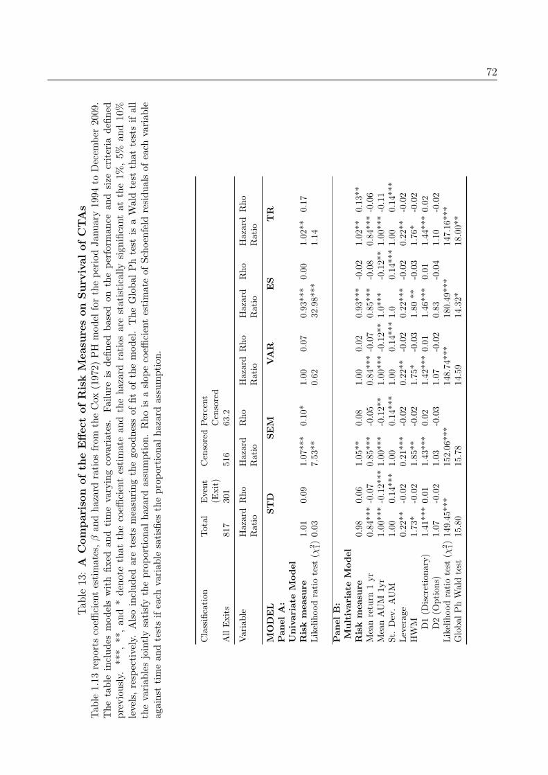
72Tab

le13:A

Compariso

nofth

eEffect

ofRiskM

easu

reson

Surv

ivalofCTAs

Tab

le1.13

reports

coeffi

cientestimates,βan

dhazardratiosfrom

theCox

(1972)PH

model

fortheperiodJanuary

1994to

Decem

ber

2009.

Thetable

includes

modelswithfixed

andtimevaryingcovariates.

Failure

isdefined

basedontheperform

ance

andsize

criteria

defined

previously.

***,

**,an

d*denotethat

thecoeffi

cientestimate

andthehazard

ratiosare

statisticallysignificantatthe1%

,5%

and10%

levels,respectively.

Alsoincluded

aretestsmeasuringthegoodnessoffitofthemodel.TheGlobalPhtest

isaWaldtest

that

testsifall

thevariab

lesjointlysatisfytheproportion

alhazardassumption.Rhois

aslopecoeffi

cientestimate

ofSchoenfeld

residualsof

each

variab

leagainst

timean

dtestsifeach

variab

lesatisfies

theproportionalhazard

assumption.

Classification

Total

Event

Cen

soredPercent

(Exit)

Cen

sored

AllExits

817

301

516

63.2

Variable

Hazard

Rho

Hazard

Rho

Hazard

Rho

Hazard

Rho

Hazard

Rho

Ratio

Ratio

Ratio

Ratio

Ratio

MODEL

STD

SEM

VAR

ES

TR

PanelA:

Univariate

Model

Riskmeasu

re1.01

0.09

1.07

***

0.10

*1.00

0.07

0.93

***

0.00

1.02

**0.17

Likelihoodratiotest

(χ2 1)0.03

7.53

**0.62

32.98*

**1.14

PanelB:

Multivariate

Model

Riskmeasu

re0.98

0.06

1.05

**0.08

1.00

0.02

0.93

***

-0.02

1.02

**0.13**

Meanreturn

1yr

0.84

***-0.07

0.85

***

-0.05

0.84

***-0.07

0.85

***

-0.08

0.84

***-0.06

MeanAUM

1yr

1.00

***-0.12*

**1.00

***

-0.12*

*1.00

***-0.12*

*1.0*

**-0.12*

*1.00

***-0.11

St.

Dev.AUM

1.00

0.14

***

1.00

0.14

***

1.00

0.14

***1.0

0.14

***1.00

0.14***

Leverag

e0.22

**-0.02

0.21

***

-0.02

0.22

**-0.02

0.22

***

-0.02

0.22

**-0.02

HW

M1.73

*-0.02

1.85

**-0.02

1.75

*-0.03

1.80

**-0.03

1.76

*-0.02

D1(D

iscretionary)

1.41

***0.01

1.43

***

0.02

1.42

***0.01

1.46

***

0.01

1.44

***0.02

D2(O

ption

s)1.07

-0.02

1.03

-0.03

1.07

-0.02

0.83

-0.04

1.10

-0.02

Likelihoodratiotest

(χ2 1)14

9.45

***

152.06

***

148.74

***

180.49

***

147.16

***

Global

PhWaldtest

15.80

15.78

14.59

14.32*

18.00*

*

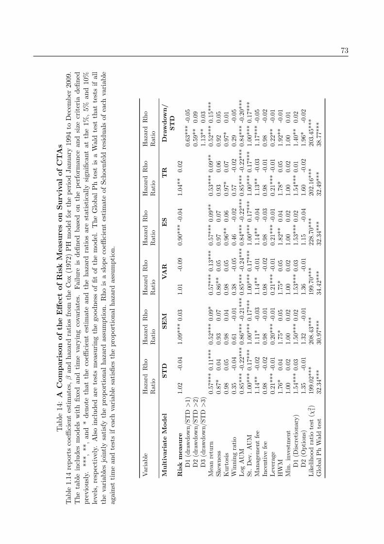
73Tab

le14:A

Compariso

nofth

eEffect

ofRiskM

easu

reson

Surv

ivalofCTAs

Tab

le1.14

reports

coeffi

cientestimates,βan

dhazardratiosfrom

theCox

(1972)PH

model

fortheperiodJanuary

1994to

Decem

ber

2009.

Thetable

includes

modelswithfixed

andtimevaryingcovariates.

Failure

isdefined

basedontheperform

ance

andsize

criteria

defined

previously.

***,

**,an

d*denotethat

thecoeffi

cientestimate

andthehazard

ratiosare

statisticallysignificantatthe1%

,5%

and10%

levels,respectively.

Alsoincluded

aretestsmeasuringthegoodnessoffitofthemodel.TheGlobalPhtest

isaWaldtest

that

testsifall

thevariab

lesjointlysatisfytheproportion

alhazardassumption.Rhois

aslopecoeffi

cientestimate

ofSchoenfeld

residualsof

each

variab

leagainst

timean

dtestsifeach

variab

lesatisfies

theproportionalhazard

assumption.

Variable

Hazard

Rho

Hazard

Rho

Hazard

Rho

Hazard

Rho

Hazard

Rho

Hazard

Rho

Ratio

Ratio

Ratio

Ratio

Ratio

Ratio

Multivariate

Model

STD

SEM

VAR

ES

TR

Dra

wdown/

STD

Riskmeasu

re1.02

-0.04

1.09

***0.03

1.01

-0.09

0.90

***-0.04

1.04

**0.02

D1(drawdow

n/S

TD

>1)

0.63***-0.05

D2(drawdow

n/S

TD

>2)

0.59**

0.09

D3(drawdow

n/S

TD

>3)

1.13**

0.03

Meanreturn

0.57

***0.11

***

0.52

***0.09

*0.57

***0.13

***

0.57

***0.09

**0.53

***0.09

**0.52***0.15***

Skew

ness

0.87

*0.04

0.93

0.07

0.86

**0.05

0.97

0.07

0.93

0.06

0.92

0.05

Kurtosis

0.98

0.05

0.98

0.04

0.98

0.05

0.96

**0.06

0.97

*0.07

0.97*

0.01

Winningratio

0.35

-0.04

0.61

-0.01

0.38

-0.05

0.46

-0.02

0.57

-0.02

0.29

-0.05

Log

AUM

0.85

***-0.22*

**0.86

***-0.21*

**0.85

***-0.24*

**0.84

***-0.22*

**0.85

***-0.22*

**0.84***-0.20***

St.

Dev.AUM

1.00

***0.17

***

1.00

***0.17

***

1.00

***0.17

***

1.00

***0.17

***

1.00

***0.17

***

1.00***0.17***

Man

agem

entfee

1.14

**-0.02

1.11

*-0.03

1.14

**-0.01

1.14

**-0.04

1.13

**-0.03

1.17***-0.05

Incentive

fee

0.98

-0.02

0.98

-0.01

0.98

-0.02

0.98

-0.03

0.98

-0.01

0.98

-0.02

Leverag

e0.21

***-0.01

0.20

***-0.01

0.21

***-0.01

0.21

***-0.01

0.21

***-0.01

0.22**

-0.01

HW

M1.76

*0.04

1.75

*0.05

1.75

*0.05

1.82

**0.04

1.78

*0.05

1.92**

-0.01

Min.investment

1.00

0.02

1.00

0.02

1.00

0.02

1.00

0.02

1.00

0.02

1.00

0.01

D1(D

iscretionary)

1.54

***0.03

1.50

***0.02

1.53

***0.03

1.53

***0.02

1.54

***0.01

1.40**

0.02

D2(O

ption

s)1.35

-0.01

1.32

-0.01

1.36

-0.01

1.15

-0.04

1.60

-0.02

1.96*

-0.02

Likelihoodratiotest

(χ2 1)

199.02

***

208.43

***

199.70

***

228.70

***

202.16

***

203.45***

Global

PhWaldtest

32.34*

**30

.97*

**34

.42*

**32

.34*

**32

.49*

**38.77***

74Tab

le15:A

Compariso

nofth

eEffect

ofRiskM

easu

reson

Surv

ivalofCTAswith

Tim

e-V

ary

ingAUM

and

Flow

Tab

le1.15

reports

coeffi

cientestimates,βan

dhazardratiosfrom

theCox

(1972)PH

model

fortheperiodJanuary

1994to

Decem

ber

2009.

Thetable

includes

modelswithfixed

andtimevaryingcovariates.

Failure

isdefined

basedontheperform

ance

andsize

criteria

defined

previously.

***,

**,an

d*denotethat

thecoeffi

cientestimate

andthehazard

ratiosare

statisticallysignificantatthe1%

,5%

and10%

levels,respectively.

Alsoincluded

aretestsmeasuringthegoodnessoffitofthemodel.TheGlobalPhtest

isaWaldtest

that

testsifall

thevariab

lesjointlysatisfytheproportion

alhazardassumption.Rhois

aslopecoeffi

cientestimate

ofSchoenfeld

residualsof

each

variab

leagainst

timean

dtestsifeach

variab

lesatisfies

theproportionalhazard

assumption.

Variable

Hazard

Rho

Hazard

Rho

Hazard

Rho

Hazard

Rho

Hazard

Rho

Hazard

Rho

Ratio

Ratio

Ratio

Ratio

Ratio

Ratio

Multivariate

Model

STD

SEM

VAR

ES

TR

Dra

wdown/

STD

Riskmeasu

re1.02

-0.02

1.10

***0.04

1.01

*-0.070.90

***-0.03

1.05

**0.03

D1(drawdow

n/S

TD

>1)

0.59

***-0.05

D2(drawdow

n/S

TD

>2)

1.01

**0.09

D3(drawdow

n/S

TD

>3)

1.71

0.06

Meanreturn

0.52

***0.09

**0.48

***0.06

0.52

***0.04

0.53

***0.08

*0.49

***0.07

0.87

***-0.08

Skewness

0.85

**0.02

0.91

0.06

0.84

**0.03

0.93

0.04

0.91

0.04

0.75

***0.13***

Kurtosis

0.98

0.05

0.97

*0.04

0.98

0.06

0.96

**0.05

0.97

**0.07

0.97

**0.00

WinningRatio

0.22

*-0.06

0.39

-0.040.25

-0.070.23

*-0.05

0.35

-0.030.05

***0.05

AUM(t)

0.99

***0.02

0.99

***0.02

0.99

***0.02

0.99

***0.02

0.99

***0.02

0.99

***0.02

Flow(t)

0.12

***-0.09

0.12

***-0.090.12

***-0.090.12

***-0.08

0.12

***-0.090.12

***-0.06

Man

agem

entfee

1.13

**-0.04

1.10

-0.051.13

**-0.031.13

**-0.06

1.11

*-0.041.09

-0.02

Incentivefee

0.98

0.00

0.98

0.02

0.98

0.00

0.98

-0.02

0.98

0.01

0.96

**-0.02

Leverag

e0.22

**-0.02

0.22

***-0.020.22

***-0.020.23

**-0.02

0.22

***-0.020.24

**-0.01

HW

M1.31

0.03

1.32

0.04

1.31

0.03

1.34

0.03

1.34

0.03

1.48

0.00

Min.investment

1.00

-0.01

1.00

-0.011.00

-0.011.00

-0.01

1.00

-0.011.00

0.00

D1(D

iscretionary)

1.55

***0.01

1.52

***0.00

1.54

***0.01

1.54

***0.01

1.55

***-0.011.61

***-0.03

D2(O

ption

s)1.48

-0.01

1.40

-0.011.49

-0.011.15

-0.03

1.73

-0.011.95

*0.02

Likelihoodratiotest

(χ2 1)

289.10

***

299.79

***

290.28

***

316.70

***

292.92

***

288.47

***

Global

PhWaldtest

12.78

13.08

13.84

13.62

13.75

20.38

75

Table 16: Survival Analysis for All StrategiesTable 1.16 reports coefficient estimates, β and hazard ratios from the Cox (1972) PH model for theperiod January 1994 to December 2009. The table includes models with fixed and time varyingcovariates and includes 12 strategies. Failure is defined based on the performance and size criteriadefined previously. ***, **, and * denote that the coefficient estimate and the hazard ratios arestatistically significant at the 1%, 5% and 10% levels, respectively. Also included are tests measuringthe goodness of fit of the model. The Global Ph test is a Wald test that tests if all the variables jointlysatisfy the proportional hazard assumption. Rho is a slope coefficient estimate of Schoenfeld residualsof each variable against time and tests if each variable satisfies the proportional hazard assumption.

Variable Hazard Rho Hazard Rho Hazard RhoRatio Ratio Ratio

Model STD TR Drawdown/STD

Risk measure 1.03 -0.05 1.06*** -0.01D1 (drawdown/STD >1) 0.51*** -0.06D2 (drawdown/STD >2) 1.01** 0.10*D3 (drawdown/STD >3) 1.00* 0.05

Mean return 0.50*** 0.10** 0.46*** 0.07* 0.52*** 0.12***Skewness 0.84** 0.01 0.90 0.03 0.76*** 0.05Kurtosis 0.98 0.07 0.97** 0.08 0.98 0.02Winning ratio 0.20* -0.06 0.31 -0.04 0.05*** -0.03AUM(t) 0.99*** 0.01 0.99*** 0.02 0.99*** 0.03Flow(t) 0.12*** -0.08* 0.12*** -0.08 0.12*** -0.08Management fee 1.16** -0.02 1.14** -0.03 1.17*** -0.03Incentive fee 0.99 0.01 0.99 0.02 1.00 0.01Leverage 0.22** -0.03 0.23** -0.03 0.22** -0.03HWM 1.15 0.02 1.19 0.02 1.08 0.01Min. investment 1.00 -0.01 1.00 -0.01 1.00 0.01

D1 (Fundamental) 0.65 0.11** 0.62* 0.11* 0.62* 0.07D2 (Technical) 0.94 0.03 0.94 0.04 0.84 0.01D3 (Disc Spread/RV) 0.80 0.08 0.84 0.08 0.86 0.04D4 (Options) 0.84 0.02 0.95 0.02 0.85 0.02D5 (Pattern Rec.) 0.66 0.06 0.66 0.06 0.59 0.06D6 (Counter Trend) 2.50* 0.04 2.50* 0.05 2.40 0.04D7 (Systematic Spread/RV) 1.03 0.09 0.99 0.10* 1.00 0.08D8 (Short-term) 0.41*** -0.06 0.42*** -0.05 0.41*** -0.07D9 (Medium-term) 0.48*** 0.07 0.48*** 0.08 0.48*** 0.05D10 (Long-term) 0.67* 0.07 0.65 0.07 0.68 0.07

Likelihood ratio test (χ21) 308.74*** 311.86*** 323.37

Global Ph Wald test 26.39 26.49 37.78

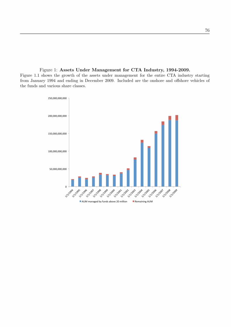
76

Figure 1: Assets Under Management for CTA Industry, 1994-2009.Figure 1.1 shows the growth of the assets under management for the entire CTA industry startingfrom January 1994 and ending in December 2009. Included are the onshore and offshore vehicles ofthe funds and various share classes.

!

"!

#"$"""$"""$"""!

%""$"""$"""$"""!

%#"$"""$"""$"""!

&""$"""$"""$"""!

&#"$"""$"""$"""!

'()!*+,+-./!01!23,/4!+056.!&"!*78875,! 9.*+7,7,-!'()!

77

Figure 2: Failed Fund with Small AUMFigure 1.2 shows VAMI and AUM for a fund that failed in terms of downside risk measures and hadnegative return in the last six months yet its assets remained stable. Such a fund would not be caughtby Liang and Park’s (2010) filter. Source: PerTrac Analytical Platform.

!

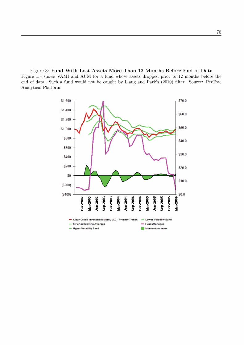
78

Figure 3: Fund With Lost Assets More Than 12 Months Before End of DataFigure 1.3 shows VAMI and AUM for a fund whose assets dropped prior to 12 months before theend of data. Such a fund would not be caught by Liang and Park’s (2010) filter. Source: PerTracAnalytical Platform.

!

79

Figure 4: Fund With Positive Average Return in the Last Six MonthsFigure 1.4 shows VAMI and AUM for a fund which experienced a large drawdown of 78.24% and aloss of assets yet in the last six months prior to termination its average return was positive. Such afund would not be caught by Liang and Park’s (2010) filter. Source: PerTrac Analytical Platform.

!

80

Figure 5: Non-Parametric Survival and Hazard CurvesFigure 1.5 shows survival and hazard curves for all 2446 funds in the sample by exit status.

0.00

0.25

0.50

0.75

1.00

0 50 100 150 200 250Duration Time (months)

ALIVE FAILURE FRAUD

LIQUIDATED LIVE

MERGED NOT REPORTING

SELF SELECTED

Kaplan−Meier Survival Curves by Graveyard Status

0.0

2.0

4.0

6.0

8

0 50 100 150 200Duration Time (months)

ALIVE FAILURE FRAUD

LIQUIDATED MERGED

NOT REPORTING SELF SELECTED

Smoothed Hazard Curve by Graveyard Status for Attrition All 2446 Funds

81

Figure 6: Non-Parametric Survival and Hazard CurvesFigure 1.6 shows survival and hazard curves for 892 funds filtered by dynamic AUM. The graphs showsurvival and hazard curves of systematic and discretionary for failed funds.

0.00

0.25

0.50

0.75

1.00

0 50 100 150 200 250Duration Time (months)

Systematic Discretionary

Kaplan−Meier Survival Curves by Strategy for 892 Failed Funds

0.0

05.0

1.0

15

0 50 100 150 200Duration Time (months)

SYSTEMATIC DISCRETIONARY

Smoothed Hazard Curve by Stategy for 892 Failed Funds

82

Figure 7: Non-Parametric Survival and Hazard CurvesFigure 1.7 shows survival and hazard curves for 892 funds filtered by dynamic AUM. The graphs showsurvival and hazard curves for failed funds across sub-strategies.

0.00

0.25

0.50

0.75

1.00

0 50 100 150 200 250Duration Time (months)

Fundamental & Technical Fundamental

Technical Disc Spread/RV

Vol Arb Options

Pattern Rec Counter Trend

Systematic Spread/RV Trend Follower

Kaplan−Meier Survival Curves by Strategy

0.0

5.1

0 50 100 150 200Duration Time (months)

Fundamental & Technical Fundamental

Technical Disc Spread/RV

Vol Arb Options

Pattern Rec Counter Trend

Systematic Spread/RV Trend Follower

Smoothed Hazard by Strategy for 892 Failed Funds

Bibliography

[1] Ackermann, C., McEnnally, R., and Ravenscraft, D. The performance of hedge

funds: Risk, return and incentives. Journal of Finance 54 (1999), 833–874.

[2] Agarwal, V., Daniel, N., and Naik, N. Role of managerial incentives and discretion

in hedge fund performance. Journal of Finance 5 (2009), 2221–2256.

[3] Agarwal, V., and Naik, N. Risks and portfolio decisions involving hedge funds. The

Review of Financial Studies 17 (2004), 63–98.

[4] Allison, P. D. Survival analysis using sas: A practical guide. SAS Institute Inc. 10, 4

(1995), 1–35.

[5] Amin, G. S., and Kat, H. Hedge funds performance 1990-2000: Do the money machines

really add value? Journal of Financial and Quantitative Analysis 38 (2003), 251–274.

[6] Andersen, P. K., and Gill, R. D. Cox’s regression model for counting processes: A

large sample study. Annals of Statistics 10, 4 (1982), 1100–1120.

[7] Aragon, G., and Qian, J. Long-term asset management and the role of high-water

marks. Working Paper Boston College (2005), 1–47.

[8] Artzner, P., Delbaen, F., Eber, J. M., and Heath, D. Coherent measures of risk.

Mathematical Finance 9, 4 (1999), 203–228.

83

BIBLIOGRAPHY 84

[9] Avramov, D., Barras, L., and Kosowski, R. Hedge fund predictability under the

magnifying glass: The economic value of forecasting individual fund returns. Working Paper

www.ssrn.com (2010), 1–58.

[10] Baba, N., and Goko, H. Hedge fund survival: Non-normal returns, capital outflows,

and liquidity. The Journal of Financial Research 32, 1 (2009), 71–93.

[11] Baquero, G., Horst, J., and Verbeek, M. Survival, look-ahead bias and persistence

in hedge fund performance. Journal of Financial and Quantitative Analysis 40 (2005),

493–517.

[12] Bhardwaj, G., Gorton, G. B., and Rouwenhorst, K. G. Fooling some of the

people all of the time: The inefficient performance and persistence of commodity trading

advisors. 2008.

[13] Billingsley, R., and Chance, D. Benefits and limitations of diversification among

commodity trading advisors. Journal of Portfolio Management 23 (1996), 65–80.

[14] Brown, S., Goetzmann, W., Liang, B., and Schwarz, C. Estimating operational

risk for hedge funds: The w-score. Financial Analysts Journal 65, 1 (2009), 43–53.

[15] Brown, S., Goetzmann, W., Liang, B., and Schwarz, C. Mandatory disclosure and

operational risk: Evidence from hedge fund registration. Journal of Finance (Forthcoming).

[16] Brown, S. J., Goetzmann, W. N., and Ibbotson, R. G. Offshore hedge funds:

Survival and performance 1989-1995. Journal of Business 72 (1999), 91–118.

[17] Brown, S. J., Goetzmann, W. N., Ibbotson, R. G., and Ross, S. A. Survivorship

bias in performance studies. Review of Financial Studies 5 (1992), 553–580.

[18] Brown, S. J., Goetzmann, W. N., and Park, J. Careers and survival: Competition

and risk in the hedge fund and cta industry. Journal of Finance 56 (2001), 1869–1886.

BIBLIOGRAPHY 85

[19] Buraschi, A., Kosowski, R., and Sritrakul, W. Incentives and endogenous risk

taking: Implications for reduced-form estimates of risk-adjusted performance in hedge funds.

Working Paper www.ssrn.com (2011), 1–53.

[20] Capocci, D., and Hubner, G. Analysis of hedge fund performance. Journal of Empirical

Finance 11 (2005), 55–89.

[21] Carpenter, J., and Lynch, A. Survivorship bias and attrition effects in measures of

performance persistence. Journal of Financial Economics 54, 8 (1999), 337–374.

[22] Chan, N., Getmansky, M., Haas, S. M., and Lo, A. W. Systematic risk and hedge

funds. in M. Carey and R. Stulz, eds. The Risks of Financial Institutions, University of

Chicago Press, Chicago (2006), 235–330.

[23] Cornish, E. A., and Fisher, R. A. Moments and cumulants in the specification of

distributions. Review of the International Statistical Institute 5, 4 (1938), 307–320.

[24] Cox, D. R. Partial likelihood. Biometrica 62, 4 (1975), 269–276.

[25] Derman, E. The premium for hedge fund lockups. Working Paper, Prisma Capital 10, 4

(2006), 1–35.

[26] Diz, F. Cta survivor and nonsurvivor: An analysis of relative performance. The Journal

of Alternative Investments 21, 1 (1999a), 57–71.

[27] Diz, F. How do ctas’ return distribution characteristics affect their likelihood of survival?

The Journal of Alternative Investments 2, 1 (1999b), 37–41.

[28] Edwards, F. R., and Caglayan, M. O. Hedge fund and commodity fund investment

styles in bull and bear markets. Journal of Portfolio Management 27, 4 (2001), 97–108.

[29] Estrada, J. The cost of equity of internet stocks: A downside risk approach. The European

Journal of Finance 10, 4 (2004), 239–254.

BIBLIOGRAPHY 86

[30] Fung, W., and Hsieh, D. A. Survivorship bias and investment style in the returns of ctas:

The information content of performance track records. Journal of Portfolio Management

24, 1 (1997b), 30–41.

[31] Fung, W., and Hsieh, D. A. Performance characteristics of hedge funds and cta

funds: Natural versus spurious biases. Journal of Quantitative and Financial Analysis

35, 3 (2000b), 291–307.

[32] Fung, W., and Hsieh, D. A. The risk in hedge fund strategies: Theory and evidence

from trend followers. The Review of Financial Studies 14, 2 (2001), 313–341.

[33] Fung, W., and Hsieh, D. A. Hedge fund benchmarks: Information content and biases.

Financial Analysts Journal 58, 1 (2002), 22–34.

[34] Fung, W., and Hsieh, D. A. Measurement biases in hedge fund performance data: an

update. Financial Analysts Journal 65, 3 (2009), 1–3.

[35] Fung, W., Hsieh, D. A., Naik, N. Y., and Ramadorai, T. Hedge funds: Perfor-

mance, risk and capital formation. Journal of Finance. 63, 1 (2008), 1777–1803.

[36] Getmansky, M., Lo, A., and Mei, S. Sifting through wreckage: Lessons from recent

hedge-fund liquidation. Journal of Investment Management 2, 3 (2004), 6–38.

[37] Gregoriou, G. N. Hedge fund survival lifetimes. Journal of Asset Management 3, 4

(2002), 237–252.

[38] Gregoriou, G. N., Hubner, G., Papageorgiou, N., and Rouah, F. Survival of

commodity trading advisors: 1990-2003. The Journal of Futures Markets 25, 8 (2005),

795–815.

[39] J. Joenvaara, R. K., and Tolonen, P. New ’stylized facts’ about hedge funds and

database selection bias. Working Paper www.ssrn.com (2012).

[40] Jarque, C. M., and Bera, A. K. Efficient tests for normality, homoscedasticity and

serial independeceof regression residuals. Economics Letters 6, 4 (1980), 255–259.

BIBLIOGRAPHY 87

[41] Kalbfleisch, J., and Prentice, R. L. The statistical analysis of failure time data.

John Wiley and Sons 2nd ed. Hoboken (2002), 1–315.

[42] Kaplan, E., and Meier, P. Nonparametric estimation from incomplete observations.

Journal of the American Statistical Association 53 (1958), 457–481.

[43] Kazemi, H., and Li, Y. Market timing of ctas: An examination of systematic ctas vs.

discretionary ctas. Journal of Futures Markets 29, 11 (2009), 1067–1099.

[44] Kosowski, R., Naik, N. Y., and Teo, M. Do hedge funds deliever alpha? a bayesian

and bootstrap analysis. Journal of Financial Economics 84, 4 (2007), 229–264.

[45] Lee, H. S. Dynamic prediction of financial distress in hedge funds and fund-of-hedge funds.

Working Paper www.ssrn.com (2010), 1–47.

[46] Liang, B. On the performance of hedge funds: 1990-1999. Financial Analysts Journal 55,

4 (1999), 72–85.

[47] Liang, B. Hedge funds: The living and the dead. Journal of Financial and Quantitative

Analysis 35, 3 (2000), 309–326.

[48] Liang, B. Hedge funds performance: 1990-1999. Financial Analysts Journal 57, 1 (2001),

11–18.

[49] Liang, B. Alternative investments: Ctas, hedge funds and fund-of-funds. Journal of

Investment Management 2, 4 (2004), 76–93.

[50] Liang, B., and Park, H. Risk measures for hedge funds: A cross-sectional approach.

European Financial Management 13, 4 (2007), 333–370.

[51] Liang, B., and Park, H. Predicting hedge fund failure: A comparison of risk measures.

Journal of Financial and Quanatitative Analysis. 45, 1 (2010), 199–222.

[52] Lo, A. Risk management for hedge funds: Introduction and overview. Financial Analysts

Journal. 57, 1 (2001), 16–33.

BIBLIOGRAPHY 88

[53] Malkiel, B. G., and Saha, A. Hedge funds: Risk and return. Financial Analysts

Journal. 61, 6 (2005), 80–88.

[54] Narang, R. K. Inside the black box. Wiley Publishing 1, 6 (2009), 80–88.

[55] Ng, M. S. The development of a forecasting model for hedge fund failure: A survival

analysis approach. Working Paper. 1, 6 (2008), 80–88.

[56] P. Lang, F. G., and Prestbo, J. Hedge fund drawdowns: An empirical analysis.

Working Paper www.ssrn.com (2006).

[57] Park, P., Tanrikulu, O., and Wang, G. Systematic global macro: Performance, risk

and correlation charachteristics. Working Paper www.ssrn.com (2009).

[58] Rami, H. A look inside the black box. Working Paper 2, 3 (2009), 6–38.

[59] Rouah, F. Competing risks in hedge fund survival. Working Paper, McGill University.

45, 1 (2005), 199–222.

[60] Schoenfeld, D. Partial residuals for the proportional hazards regression model.

Biometrika 69 (1982), 239–241.

[61] Shefrin, H., and Statman, M. The disposition to sell winners too early and ride losers

too long: Theory and evidence. Journal of Finance XL, 3 (1985).

[62] Sirri, E., and Tufano, P. Costly search and mutual fund flows. Journal of Finance 53

(1998), 1589–1622.

[63] Spurgin, R. A study of survival: Commodity trading advisors: 1988-1996. The Journal

of Alternative Investments. 2, 3 (1999), 16–22.

[64] Taleb, N. N. Bleed or blowup? why do we prefer asymmetric payoffs? Journal of

Behavioural Finance 5, 4 (2004), 2–7.

BIBLIOGRAPHY 89

[65] Xu, X. E., Liu, J., and Loviseck, A. L. Hedge fund attrition, survivorship bias and

performance: Perspectives from the global financial crisis. Working Paper. 2, 3 (2010),

16–22.