surjections in locally convex spaces · in chapter 4, we will construct new spaces out of other...
TRANSCRIPT
Ghent UniversityFaculty of Sciences
Department of Mathematics
Surjections in locally convex spaces
by
Lenny Neyt
Supervisor: Prof. Dr. H. Vernaeve
Master dissertation submitted to the Faculty of Sciences to obtain the
academic degree of Master of Science in Mathematics: Pure Mathematics.
Academic Year 2015–2016
Preface
For me, in the past five years, mathematics metamorphosed from an interestinto my greatest passion. I find it truly fascinating how the combination oflogical thinking and creativity can produce such rich theories. Hopefully,this master thesis conveys this sentiment.
I hereby wish to thank my promotor Hans Vernaeve for the support andadvice he gave me, not only during this thesis, but over the last three years.Furthermore, I thank Jasson Vindas and Andreas Debrouwere for their helpand suggestions. Last but not least, I wish to express my gratitude towardmy parents for the support and stimulation they gave me throughout myentire education.
The author gives his permission to make this work available for consultationand to copy parts of the work for personal use. Any other use is bound by therestrictions of copyright legislation, in particular regarding the obligation tospecify the source when using the results of this work.
Ghent, May 31, 2016 Lenny Neyt
i
Contents
Preface i
Introduction 1
1 Preliminaries 31.1 Topology . . . . . . . . . . . . . . . . . . . . . . . . . . . . . 31.2 Topological vector spaces . . . . . . . . . . . . . . . . . . . . 71.3 Banach and Frechet spaces . . . . . . . . . . . . . . . . . . . 111.4 The Hahn-Banach theorem . . . . . . . . . . . . . . . . . . . 131.5 Baire categories . . . . . . . . . . . . . . . . . . . . . . . . . . 151.6 Schauder’s theorem . . . . . . . . . . . . . . . . . . . . . . . . 16
2 Locally convex spaces 182.1 Definition . . . . . . . . . . . . . . . . . . . . . . . . . . . . . 182.2 Topological aspects of locally convex spaces . . . . . . . . . . 24
2.2.1 Hausdorff . . . . . . . . . . . . . . . . . . . . . . . . . 242.2.2 Convergence . . . . . . . . . . . . . . . . . . . . . . . 252.2.3 Continuity of linear operators . . . . . . . . . . . . . . 262.2.4 Boundedness . . . . . . . . . . . . . . . . . . . . . . . 30
2.3 Quotient spaces . . . . . . . . . . . . . . . . . . . . . . . . . . 342.4 Hahn-Banach in locally convex spaces . . . . . . . . . . . . . 362.5 Application: Kakutani’s fixed point theorem . . . . . . . . . . 412.6 Completions . . . . . . . . . . . . . . . . . . . . . . . . . . . . 43
3 Duality theory 463.1 Classification of admissible topologies . . . . . . . . . . . . . 463.2 Boundedness in duality theory . . . . . . . . . . . . . . . . . 543.3 Reflexivity . . . . . . . . . . . . . . . . . . . . . . . . . . . . . 563.4 Continuity and surjectivity of linear maps . . . . . . . . . . . 623.5 Mackey spaces . . . . . . . . . . . . . . . . . . . . . . . . . . 683.6 Equicontinuous sets . . . . . . . . . . . . . . . . . . . . . . . 68
ii
iii
4 Projective and inductive topologies 724.1 Definitions . . . . . . . . . . . . . . . . . . . . . . . . . . . . . 724.2 Bornological spaces . . . . . . . . . . . . . . . . . . . . . . . . 774.3 Schwartz spaces . . . . . . . . . . . . . . . . . . . . . . . . . . 804.4 The open mapping theorem . . . . . . . . . . . . . . . . . . . 854.5 Imbedding spectra and (LF)-spaces . . . . . . . . . . . . . . . 89
5 Frechet spaces and (DF)-spaces 935.1 Metrizable spaces . . . . . . . . . . . . . . . . . . . . . . . . . 935.2 (DF)-spaces . . . . . . . . . . . . . . . . . . . . . . . . . . . . 985.3 Weakly compact imbedding spectra . . . . . . . . . . . . . . . 102
6 Surjections of Frechet Spaces 1086.1 Characterizing surjectivity . . . . . . . . . . . . . . . . . . . . 1086.2 Surjectivity between Frechet spaces . . . . . . . . . . . . . . . 1116.3 Applications . . . . . . . . . . . . . . . . . . . . . . . . . . . . 117
6.3.1 Formal power series and Taylor expansions . . . . . . 1176.3.2 The existence of C8 solutions of a linear partial dif-
ferential equation . . . . . . . . . . . . . . . . . . . . . 121
7 Surjectivity of dual mappings 1247.1 Surjectivity of the dual map . . . . . . . . . . . . . . . . . . . 1247.2 Acyclic (LF)-spaces . . . . . . . . . . . . . . . . . . . . . . . . 1267.3 Retractive (LF)-spaces . . . . . . . . . . . . . . . . . . . . . . 1337.4 Inductive limits of Frechet-Montel spaces . . . . . . . . . . . 137
Conclusion 142
Indication of the used sources 144
A Nederlandstalige samenvatting 145
B Distributions 147B.1 The distribution space D1pΩq . . . . . . . . . . . . . . . . . . 147B.2 Differentiation . . . . . . . . . . . . . . . . . . . . . . . . . . 148B.3 Fourier transform . . . . . . . . . . . . . . . . . . . . . . . . . 149B.4 Convolution . . . . . . . . . . . . . . . . . . . . . . . . . . . . 150
Bibliography 152
Index 154
Introduction
In mathematics, it is desirable to know whether or not a problem is generallysolvable. For instance, consider the partial differential equation¸
kPNnan
B
Bx
kφ ψ, (1)
over some space of sufficiently differentiable functions. We wonder if (1) issolvable for each ψ, i.e. if we put
D :¸kPNn
an
B
Bx
k,
we ask ourselves if for each ψ there is a φ such that Dφ ψ. Now, since Dis a map, this will exactly be the case if D is a surjection. While this specificproblem has been studied extensively (we refer to [2] for a nice overview),we may look at it in a more comprehensive framework.
In general, suppose E and F are topological vector spaces, and A :E Ñ F is a continuous linear map, then the problem we will investigatethroughout this master thesis is whether or not A is a surjection. This isexactly the case if the image of A is both closed and dense in F . For thelatter condition we will find a general characterization, namely injectivityof the transpose map, but for closedness we will need more structure on thespaces to find verifiable requirements. This is why an extensive knowledgeabout the spaces used in functional analysis is vital, and we will thereforespend a great amount of time on it.
In chapter 1, we discuss some preliminary analytic concepts and resultswe expect the reader to be familiar with and may be bypassed at first, sinceall used results are referred to. On top of these results, we also expect thereader to be familiar with some basic notions in the field of algebra, such asvector spaces and groups.
In chapter 2, we introduce the locally convex spaces, which are the gen-eral spaces we will be working with. These spaces can be seen as a vectorspaces equipped with a family of continuous seminorms. The chapter mainlyserves to establish the structure of these spaces, in order for it to be easyapplicable in the sequel. Nonetheless, we will already utilize these results to
1

2
give an application in the form of a fixed point theorem due to S. Kakutani[5].
In chapter 3, we will be looking at the duals of locally convex spacesand study the possible ways to topologize them. Via this, one can discovera remarkable interplay between a space and its dual, which will greatlyincrease our understanding of the locally convex spaces. Our first generalcharacterization of the surjectivity problem will also be made here.
In chapter 4, we will construct new spaces out of other locally convexspaces, using projective and inductive topologies. This will pave the way formany new categories of spaces, such as the bornological spaces. The mainresult of this chapter is an extension of the open mapping theorem, a toolthat is critical in our search for surjections, to more general spaces, due tode Wilde [18].
In chapter 5, we will focus on Frechet spaces and their duals. SinceFrechet spaces are both complete and metrizable, they will have some strongproperties, which we will apply in the chapter following it to characterizesurjectivity between Frechet spaces.
In chapter 6, an equivalent condition for the surjectivity of a map be-tween a Mackey webbed space and an ultra-bornological space, under certainconditions, is shown. This will be an extension of a result due to S. Banach.In particular, the characterization will work for a map between two Frechetspaces. Said conditions will be used to discuss two applications: an easyproof of a classical theorem by E. Borel and a characterization of C8 solu-tions of linear partial differential equations.
In chapter 7, our perspective will shift by looking at the surjectivityproblem for the transpose map. As it will turn out, this problem is linkedwith the notion of acyclicness, following the definition of Palamodov [8].Because of this, we will investigate equivalent definitions for this notion,which were discovered by Wengenroth [17].
Chapter 1
Preliminaries
This chapter serves as a quick reference to a list of important notions andresults that will be used in the sequel. We expect the reader to be familiarwith most of what will be discussed, hence not all results shall be given aproof. In order to confirm that all that is reviewed is fact, we refer to thebooks of Meise-Vogt [7] and Treves [15].
1.1 Topology
Definition 1.1.1. Given a set E, a filter F is a family of subsets of Esubmitted to the following three conditions:
(F1) the empty set H does not belong to the family F ;
(F2) if A1 and A2 belong to F , then A1 XA2 P F ;
(F3) any set which contains a set belonging to F should also belong to F .
Definition 1.1.2. Let E be a set and suppose that for each x P E, there isa filter Fx of E such that:
(a) for each U P Fx, we have x P U ;
(b) if U P Fx, then there is a V P Fx contained in U with the property thatfor each y P V , we have V P Fy.
This family of filters is called a topology on E, and a set equipped witha topology is called a topological space. Each U P Fx is called a x-neighborhood.
Notation 1.1.3. For a topological space E and a point x P E, the familyof x-neighborhoods will also be denoted by UxpEq.
We may now introduce the following list of notions.
3
CHAPTER 1. PRELIMINARIES 4
Definition 1.1.4. Let E be a topological space.
1. A subset U E is called open if U P UxpEq for each x P U .
2. A subset V E is called closed if EzV is open.
3. A point x of a subset W E is called an interior point of W if thereis a U P UxpEq such that U W . The set of all interior points of Wis called the interior of W and is denoted by W .
4. The closure W of a subset W E is the intersection of all closed setsthat contain W . As is known, this is again a closed subset of E.
5. A subset V E is said to be dense in E if V E.
Remark 1.1.5. Sometimes we will denote a topological space E by pE, tq,where t will denote the topology of E. Said t will be the family of all opensets in E. Recall that this family determines the topology.
In order to understand a topology, it is not necessary to know eachelement in each filter, but to find a family that generates it.
Definition 1.1.6. Let G be a family of subsets of a set E, so that
(i) H R G;
(ii) given A1, A2 P G, there is a A3 P G such that A3 A1 XA2.
The filter generated by the filter basis G is then:
FG : tU E : A U for some A P Gu .
Then FG will in fact be a filter.
Definition 1.1.7. A family of subsets B is called a filter basis for the filterF over a set E, if
(BF1) B F ;
(BF2) every subset of E belonging to F contains some subset of B.
One easily sees that B generates the filter F .Should E be a topological space and x P E, a filter base for UxpEq will
also be called a x-neighborhood basis.
Definition 1.1.8. Let E be a topological space and F be a subset of E.Consider for each x P F the family
Bx : tU X F : U P UxpEqu.
Then clearly Bx will be a filter basis, hence it generates a filter around x.This induces a topology on F , which is called the induced topology.
CHAPTER 1. PRELIMINARIES 5
Definition 1.1.9. A topological space E is called first countable if foreach x P E, UxpEq is generated by a countable filter basis.
To a certain degree, a topology is a way of saying when a sequence con-verges. However, if the space is not first countable, we will need somethinga little bit more general than sequences to determine the topology.
Definition 1.1.10. Let pT,¤q be a partially ordered set1 that is directed,i.e. for every σ, τ P T there exists a υ P T such that σ ¤ υ and τ ¤ υ. Anet of a set E is a family pxτ qτPT of elements xτ of E.
Remark 1.1.11. Since pN,¤q is a directed partially ordered set, each se-quence is a net.
Definition 1.1.12. A net pxτ qτPT in a topological space E is said to con-verge to x if for each U P UxpEq there exists a τ0 P T such that xτ P U foreach τ ¥ τ0. We will denote this by xτ Ñ x and call x a limit of the netpxτ qτPT .
Remark 1.1.13. A convergent net need not have a unique limit. Considerfor instance the trivial topology, where each point only has the entire spaceas neighborhood. Then each net will converge to each point. Uniqueness ofthe limit can only be guarantied if the points of a topological space can besufficiently ’separated’.
Definition 1.1.14. A topological space E is called Hausdorff if for eachpair of different points x, y P E there are U P UxpEq and V P UypEq suchthat U X V H.
Lemma 1.1.15. A convergent net in a Hausdorff topological space has aunique limit.
In practice, closedness will frequently be verified through convergence.
Lemma 1.1.16. Let V be a subset of E, then
V tx P E : there exists a net pxτ qτPT in V with xτ Ñ xu.
In particular, V is closed if and only if for every convergent net of elementsin V , its limit is also in V .
1A partially ordered set pP,¤q is a set P together with a binary relation ¤ over P ,which satisfies for all a, b, c P P
1. a ¤ a;
2. if a ¤ b and b ¤ a then a b;
3. if a ¤ b and b ¤ c then a ¤ c.

CHAPTER 1. PRELIMINARIES 6
As is frequently done in mathematics, it is desirable to compare certainstructures with each other through mappings. In the case of topologicalspaces, this is done in the form of continuity.
Definition 1.1.17. Let E and F be topological spaces and f : E Ñ Fbe a mapping. The map f is said to be continuous at x P E if for eachV P UfpxqpF q, we have f1pV q P UxpEq.
The map is said to be continuous if it is continuous at all points in E.It is called a homeomorphism if it is bijective and f and f1 are bothcontinuous.
The map f is called open if for each open set U of E, fpUq will be openin F .
Lemma 1.1.18. A map f : E Ñ F between two topological spaces E andF is continuous at x P E if and only if for every net pxτ qτPT converging tox, the net pfpxτ qqτPT converges to fpxq.
The next topological notion we wish to discuss is that of compactness.
Definition 1.1.19. A topological space E is said to be compact if eachopen covering of E has a finite subcovering. A subset F of a topologicalspace E is said to be compact if F is compact in the induced topology.
Properties 1.1.20. (a) A topological space E is compact if and only if foreach family pAiqiPI of closed subsets Ai of E such that
iPI Ai H,
there exists a finite subset J of I such thatiPJ Ai H.
(b) Every closed subset F of a compact topological space E is compact.
Proposition 1.1.21. Let E and F be topological spaces and let f : E Ñ Fbe a continuous map. Then:
1. if E is compact then so is fpEq;
2. if E is compact and f is bijective, then f is a homeomorphism.
Definition 1.1.22. A subset F of a topological space E is called relativelycompact if its closure E is compact.
One important result about compact sets is Tychonoff’s theorem, whichdiscusses compactness in the product space. Let us first recall what exactlya topological product is.
Definition 1.1.23. Let pEiqiPI be a family of topological spaces. Considerthe set E :
±iPI Ei and for each i P I the canonical map πi : E Ñ Ei.
Take x P E and define the following family
Bx :
#¹iPI
Ui : Ui P UπipxqpEiq for all i P I, Ui Ei only for finitely many i P I
+.

CHAPTER 1. PRELIMINARIES 7
These sets will generate a topology on E, which is called the producttopology on E. It will be the coarsest topology for which all the canonicalmaps are continuous.
Theorem 1.1.24 (Tychonoff). Let pEiqiPI , I H, be a family of topolog-ical spaces. The topological product
±iPI Ei is compact if and only if Ei is
compact for each i P I.
Proof. See [7], theorem 4.3 on page 20.
A notion that is related to compactness is that of sequential compactness.
Definition 1.1.25. A subset K of a topological vector space E is calledsequentially compact if each infinite sequence in K has a convergentsubsequence that converges to an element ofK. A subset is called relativelysequentially compact if its closure is sequentially compact.
The following lemma will be a useful tool to construct specific spaces.
Lemma 1.1.26. Let Ω be an open subset of Rn. There is a sequence ofcompact subsets K1,K2, . . . ,Kr, . . . of Ω with the following properties:
(a) for each j 1, 2, . . ., Kj is contained in the interior of Kj1;
(b) the union of the sets Kj is equal to Ω.
Proof. See [15], lemma 10.1 on page 87.
1.2 Topological vector spaces
Functional analysis is the study of topological vector spaces, which combinesthe theories of topology and algebra. Suppose we have a vector space E,then how do we topologize it? Of course, we could consider E as a setand equip it with a random topology, but then we would lose the algebraicinformation. Since a vector space is determined by its two vector spaceoperations, it is topologically natural to wish for them to be continuous.
Notation 1.2.1. We denote by K either of the fields R or C.
Definition 1.2.2. A topological vector space E is a K-vector space en-dowed with a topology for which the vector space operations are continuous.
If for a topology t on a K-vector space E, we have that pE, tq is a topo-logical vector space, we call t a vector space topology.
Definition 1.2.3. Let E and F be topological vector spaces and A : E Ñ Fbe a linear bijective map. If A is a homeomorphism, then we call A anisomorphism and we write E F .

CHAPTER 1. PRELIMINARIES 8
Since addition is continuous on a topological vector space E, the trans-lation operator Tt : E Ñ E, via a point t P E, defined by Ttpxq x t willbe a continuous, linear bijective map. Since T1
t Tt, it follows that theinverse map is also continuous, hence Tt is an isomorphism. An importantconsequence of this is that the entire topology of E is determined by itsneighborhoods of zero.
In a similar fashion, the dilation operator Da : E Ñ E, for a a P Kzt0u,defined by Dapxq ax, is also an isomorphism.
Definition 1.2.4. Let E be a K-vector space. A subset A of E is calledcircled, if for each x P A and λ P K with |λ| ¤ 1, we have that λx P A.
A subset A of E is said to be absorbing if to every x P E there is anumber cx ¡ 0 such that, for all λ P K, |λ| ¤ cx, we have λx P A.
One can now find the following characterization of topological vectorspaces (see [15], theorem 3.1 on page 21).
Theorem 1.2.5. A filter F on a K-vector space E is the filter of neighbor-hoods of the origin in a vector space topology on E if and only if it has thefollowing properties:
(1) the origin belongs to every U P F ;
(2) to every U P F there is a V P F such that V V U ;
(3) for every U P F and every λ P K, λ 0, we have λU P F ;
(4) every U P F is absorbing;
(5) every U P F contains some V P F which is circled.
In this thesis, we will be working with locally convex spaces. These aretopological vector spaces such that their zero neighborhood basis is gen-erated by a filter basis of convex sets. Let us therefore recall the exactdefinition of convexity.
Definition 1.2.6. Let E be a K-vector space and U be a subset of E.Then U is called convex if for each x, y P U and t P r0, 1s, we have thattx p1 tqy P U .
The subset U is called absolutely convex if for each x, y P U and eachλ, µ P K such that |λ| |µ| ¤ 1 we have λx µy P U .
It is not hard to see that the intersection of arbitrarily many (absolutely)convex sets is again (absolutely) convex. Therefore, for every subset U of aK-vector space E there exists a smallest (absolutely) convex set V containingU . The smallest convex set that contains U is called the convex hull of U ,and is denoted by convpUq. One can show that
conv pUq
#n
i1
λixi : λi P R, xi P U, 1 ¤ j ¤ n,n
i1
λi 1, n P N
+.

CHAPTER 1. PRELIMINARIES 9
Analogously, the smallest absolutely convex set that contains U is calledthe absolutely convex hull of U , denoted by ΓU , and is given by
ΓU
#n
i1
λixi : λi P K, xi P U, 1 ¤ j ¤ n,n
i1
|λi| ¤ 1, n P N
+.
Definition 1.2.7. A topological vector space E for which U0pEq is generatedby a filter basis consisting of convex sets is called locally convex.
Because of the algebraic structure of topological vector spaces, we cannow easily introduce several notions. One of these is completeness.
Definition 1.2.8. Let E be a topological vector space. A net pxτ qτPT issaid to be a Cauchy net if for each U P U0pEq there exists a τU P T suchthat, for all σ, τ ¥ τU , we have xσ xτ P U .
A subset F of E is said to be complete, resp. sequentially complete,if every Cauchy net, resp. every Cauchy sequence, in F has a limit in F .
A topological vector space E does not necessarily need to be complete.However, should E be Hausdorff, one can always find a complete topologicalvector space where E can be seen as a dense subspace. This is called acompletion.
Definition 1.2.9. Let E be a topological vector space. A completion ofE is a pair p pE, jq, consisting of a complete topological vector space pE and acontinuous linear injective map j : E Ñ pE such that jpEq is dense in pE andj1 : jpEq Ñ E is continuous.
The following result is by no means trivial, and we do not expect thereader to solve it. Nonetheless, we will not present a proof here, since it won’tbe applied in this general context. In chapter 2 (see proposition 2.6.3), anargument for the case of locally convex spaces will be presented.
Theorem 1.2.10. Every Hausdorff topological vector space E has a unique(with respect to isomorphisms) completion.
Proof. See [15], theorem 5.2 on page 41.
Now that we know a completion exists, we may introduce the followingdefinition.
Definition 1.2.11. A subset A of a Hausdorff topological vector space E issaid to be precompact if A is relatively compact when viewed as a subsetof the completion pE of E.
Lemma 1.2.12. The following properties of a subset K of a Hausdorfftopological vector space are equivalent:
CHAPTER 1. PRELIMINARIES 10
(a) K is precompact;
(b) given any V P U0pEq, there is a finite family of points of K, x1, . . . , xr,such that the sets xi V form a covering of K.
Proof. See [15], proposition 6.9 on page 55.
We now list some results on topological vector spaces that will be usedin the sequel.
Properties 1.2.13. Let E be a Hausdorff topological vector space and A,Bbe subsets of E.
(a) If A and B are absolutely convex and compact, then ΓpA Y Bq is alsocompact.
(b) If A is closed and B is compact, then AB is closed.
(c) If A is convex, absolutely convex or circled, then so is A.
(d) A is compact if and only if it is precompact and complete.
(e) If A is (pre)compact then so is ΓA.
Proof. (a), (b) and (c) are easy exercises. A proof to (d) can be found in[15] on page 54. Then (e) follows from (d) and lemma 1.2.12.
The structure of a finite dimensional Hausdorff topological vector spaceis, up to an isomorphism, the usual one, namely a product of K.
Theorem 1.2.14. Let E be a finite dimensional Hausdorff topological vectorspace. Then:
1. E is isomorphic to Kd, where d dimE;
2. every linear functional on E is continuous;
3. every linear map of E into any topological vector space F is continuous.
Proof. See [15], theorem 9.1 on page 79.
Corollary 1.2.15. Every finite dimensional linear subspace of a Hausdorfftopological vector space is closed.
Proof. See [15], corollary 2 on page 80.
CHAPTER 1. PRELIMINARIES 11
1.3 Banach and Frechet spaces
Definition 1.3.1. Let E be a set. A metric on E is a function d : EE ÑR that meets the following properties:
(M1) dpx, yq 0 if and only if x y;
(M2) dpx, yq dpy, xq for all x, y P E (symmetry);
(M3) dpx, zq ¤ dpx, yq dpy, zq for all x, y, z P E (triangle inequality).
A metric space pE, dq is a nonempty set E together with a metric d on E.In the sequel we shall often speak of metric spaces E without mentioningthe specific metric d. For each x P E and ε ¡ 0 we may consider the set
Bpx, εq : ty P E : |dpx, yq| εu.
These sets generate a topology on E for which d is continuous. Hence eachmetric space can be seen as a topological space. Even more, by theorem1.2.5, a metric space will be a topological vector space.
Lemma 1.3.2. For a subset M of a complete metric space E the followingstatements are equivalent:
1. M is relatively compact;
2. M is precompact;
3. M is relatively sequentially compact.
Proof. See [7], corollary 4.10 on page 22.
Definition 1.3.3. Let E be a K-vector space. A norm on E is a function‖‖ : E Ñ R with the following properties:
(N1) ‖λx‖ |λ| ‖x‖ ,@λ P K, x P E;
(N2) ‖x y‖ ¤ ‖x‖ ‖y‖ ,@x, y P E (triangle inequality);
(N3) ‖x‖ 0 if and only if x 0.
Should ‖‖ only satisfy (N1) and (N2) it is called a seminorm on E.A normed space pE, ‖‖q is a K-vector space E, on which a norm ‖‖ is
defined. In the sequel we will often not mention the norm on E explicitly.
If E is a normed space, then we can define a metric d on E, which iscalled the canonical metric, by
dpx, yq : ‖x y‖ , x, y P E.
CHAPTER 1. PRELIMINARIES 12
Definition 1.3.4. A locally convex, complete metric space is called a Frechetspace. A normed space that is complete under its canonical metric is calleda Banach space.
It’s clear that every Banach space is a Frechet space. In order to showthat a Frechet space is in fact a more general notion than a Banach space,we will now give an example of a space that is Frechet but not Banach. Forthis, we first need a lemma.
Lemma 1.3.5. Let pEn, ‖‖nqnPN be a sequence of normed spaces. A metricis defined on E
±nPNEn by
dpx, yq :8
n1
1
2n‖xn yn‖n
1 ‖xn yn‖nx pxnqnPN, y pynqnPN P E.
The following properties hold for pE, dq.
1. A sequence pxpjqqjPN in E is convergent (resp. Cauchy) in pE, dq if
and only if for each n P N, pxpjqn qjPN is convergent (resp. Cauchy).
2. pE, dq is a locally convex metric linear space.
3. If each space pEn, ‖‖nq is complete, then pE, dq is a Frechet space. IfEn t0u for infinitely many n P N, then E is not a Banach space.
Proof. The function d is well defined since°8n1 12n converges. It is not
hard to see that d satisfies (M1) and (M2). In order to prove that d satisfies(M3), and consequently that it is a metric on E, we look at the functiont ÞÑ t
1t . This function monotonically increases on r0,8r (its derivative
1p1 tq2 is strictly positive), which implies
‖xn yn‖n1 ‖xn yn‖n
¤‖xn zn‖n ‖zn yn‖n
1 ‖xn zn‖n ‖zn yn‖n
¤‖xn zn‖n
1 ‖xn zn‖n
‖zn yn‖n1 ‖zn yn‖n
,
for some z pznqnPN P E. From this (M3) follows easily.The first property is a direct consequence from the definition of d. In
order to prove that pE, dq is locally convex, we take an arbitrary a P Eand ε ¡ 0. Choose a k P N such that 2k1ε ¡ 1. For all x P E with‖xn an‖n
ε2 for 1 ¤ n ¤ k we then have
dpx, aq k
n1
1
2n‖xn an‖n
1 ‖xn an‖n
8
nk1
1
2n‖xn an‖n
1 ‖xn an‖n
k
n1
1
2nε
2
8
nk1
1
2n ε
2
1
2k ε.
CHAPTER 1. PRELIMINARIES 13
This implies that the set
V paq :!x P E : ‖xn an‖n
ε
2for 1 ¤ n ¤ k
)is contained in Bpa, εq. Let x pxnqnPN and y pynqnPN both be containedin V paq and take λ P r0, 1s; then we have for each n P N with 1 ¤ n ¤ k:
‖λxn p1 λqyn an‖n ¤ ‖λxn λan‖n ‖p1 λqyn p1 λqan‖n ε
2.
Hence V paq is convex, and since it is also open we conclude that pE, dq islocally convex, so that (2) follows.
The first statement in (3) is a direct consequence of (1) and (2). Say thatEn t0u for infinitely many n P N, and assume that there is a continuousnorm ‖‖ on pE, dq for which d would be its canonical metric (i.e. pE, dqwould be a Banach space). By our previous discussion, there exists an ε ¡ 0and k P N such that
V p0q Bp0, εq tx P E : ‖x‖ ¤ 1u .
We now choose m P N, m ¡ k such that Em t0u, and take a xm P Emwith xm 0. We define in E the element ξ : pδmn xmqnPN, with δmn theKronecker delta function. Then for each λ ¡ 0 we have that λξ P V p0q sothat λ ‖ξ‖ ¤ 1. Hence ‖ξ‖ 0, contradicting that ξ 0.
Example 1.3.6. The space ω KN of all sequences in K is, by lemma1.3.5, a Frechet space, equipped with the metric
d : px, yq ÞÑ8
n1
1
2n|xn yn|
1 |xn yn|x pxnqnPN, y pynqnPN P ω.
However, again by lemma 1.3.5, pω, dq is not a Banach space.
1.4 The Hahn-Banach theorem
Definition 1.4.1. Let E and F be normed spaces. We define
LpE,F q : tA : E Ñ F : A is linear and continuousu .
We denote LpEq : LpE,Eq.
For all normed spaces E,F we can give LpE,F q the structure of a K-vector space by defining for each A,B P LpE,F q and λ P K the linear mapsA B, λA : E Ñ F as pA Bqx Ax Bx, pλAqx λpAxq. Even moreso, LpE,F q can be equipped with a norm ‖‖, called the operator norm,defined as
‖A‖ sup‖x‖¤1
‖Ax‖ sup‖x‖1
‖Ax‖ .
One can now prove the following result.
CHAPTER 1. PRELIMINARIES 14
Proposition 1.4.2. Let E and F be normed spaces.
1. LpE,F q, equipped with the operator norm, is a normed space.
2. If F is a Banach space, then so is LpE,F q.
Definition 1.4.3. For a normed space E we call LpE,Kq the dual spaceof E, and it is denoted by E1. The elements of E1 are called continuouslinear functionals or continuous linear forms. Due to proposition 1.4.2,the dual space of a normed space is always a Banach space.
Notation 1.4.4. For a K-vector space E, we denote the set of all linearmaps A : E Ñ K by E. Notice that in a similar way as for E1, we can turnE into a K-vector space. The elements in E are called linear functionalsor linear forms.
We want to formulate the Hahn-Banach theorem in its most generalform. In order to do this, we need the following definition.
Definition 1.4.5. A sublinear functional p on a K-vector space E is areal valued function such that
1. ppλxq λppxq for all λ P R, x P E;
2. ppx yq ¤ ppxq ppyq for all x, y P E.
For example, every seminorm is a sublinear functional.
Remark 1.4.6. Let p be a sublinear funtional on a K-vector space E. Thenwe have
ppxq pp2x xq ¤ pp2xq ppxq 2ppxq ppxq,
i.e. ppxq ¤ ppxq.
Before we state the Hahn-Banach theorem, it is interesting to note thatin order to prove said theorem we need Zorn’s lemma, which is equivalentto the axiom of choice. Since it will be applied in the sequel, we formulateit here.
Theorem 1.4.7 (Zorn’s lemma). Let pL,¤q be a nonempty partially orderedset. Assume that every totally ordered family2 pxiqiPI in L has an upper limitin L (i.e. x P L such that x ¥ xi for each i P I). Then L has a maximalelement (i.e. x P L such that x ¢ y for every y P L).
Theorem 1.4.8 (Hahn-Banach). Let E be a K-vector space, p be a sublinearfunctional on E, F ¤ E and let φ0 : F Ñ R be a linear functional such thatφ0pxq ¤ ppxq for all x P F . Then there exists a linear functional φ on Esuch that φ extends φ0 and φpxq ¤ ppxq for all x P E.
2A totally ordered set is a partially ordered set pT,¤q such that for any a, b P T ,either a ¤ b or b ¤ a.
CHAPTER 1. PRELIMINARIES 15
We shall also use the following alternative formulation of the Hahn-Banach theorem.
Proposition 1.4.9. Let E be a K-vector space, p be a seminorm on E,F ¤ E and let φ0 : F Ñ K be a linear functional such that |φ0pxq| ¤ ppxqfor all x P F . Then there exists a linear functional φ on E that extends φ0
such that |φpxq| ¤ ppxq for all x P E.
Corollary 1.4.10. Let E be a K-vector space, p a seminorm on E andz P E. There exists a linear form φ on E such that φpzq ppzq and|φpxq| ¤ ppxq for all x P E.
Proposition 1.4.11. Let E be a normed space, F ¤ E and φ P F 1. Thenthere exists a Φ P E1 such that Φ|F φ and ‖φ‖ ‖Φ‖.
Proposition 1.4.12. Let E be a normed space and x P E. There exists aφ P E1 such that φpxq ‖x‖ and ‖φ‖ ¤ 1. In particular, for each x P E wehave
‖x‖ max |φpxq| : φ P E1, ‖φ‖ ¤ 1
(.
1.5 Baire categories
Definition 1.5.1. Let E be a topological space and M a subset of E. Mis said to be nowhere dense in E if M has no interior points. If M is acountable union of nowhere dense sets, then M is said to be of I-categoryin E. M is said to be of II-category in E if it is not of the I-category.
Definition 1.5.2. A topological space E is called a Baire space if everynonempty open subset of E is of II-category in E.
Proposition 1.5.3. Let E be a topological space. Then the following areequivalent:
1. E is a Baire space;
2. any intersection of countably many dense subsets of E is dense in E;
3. the interior of every union of countably many closed nowhere densesubsets of E is empty;
4. when the union of countably many closed subsets of E has an interiorpoint, then one of the closed subsets must have an interior point.
Theorem 1.5.4 (Baire). A complete metric space is a Baire space.
Proof. See [7], theorem 3.3 on page 14.
We will now list several consequences of Baire’s theorem, which are allshown in [7], chapter 8.
CHAPTER 1. PRELIMINARIES 16
Proposition 1.5.5. Let E and F be metric linear spaces and A : E Ñ Fbe a continuous linear map. If E is complete and ApEq is of II-category inF then A is open and surjective.
Theorem 1.5.6 (Uniform boundedness principle). Let E be a Banach space,F be a normed space and A LpE,F q be such that supAPA ‖Ax‖ 8 forevery x P E. Then supAPA ‖A‖ 8.
Proof. For every t ¡ 0 define
Vt :
"x P E : sup
APA‖Ax‖ ¤ t
*
£APA
tx P E : ‖Ax‖ ¤ tu .
Then Vt is closed and absolutely convex for every t ¡ 0. By the hypothesis,we have that E
nPN Vn. Using Baire’s theorem 1.5.4, we find an m P N
such that Vm has an interior point ξ. Choose an ε ¡ 0 such that Bpξ, εq Vm. By the absolute convexity of Vm we have Bpξ, εq Bpξ, εq Vm Vm. This implies
Bp0, εq 1
2Bpξ, εq
1
2Bpξ, εq
1
2Vm
1
2Vm Vm.
For every A P A we now have:
‖A‖ 1
εsup t‖Ax‖ : ‖x‖ ¤ εu ¤
m
ε.
Corollary 1.5.7. If E is a normed space and M is a subset of E such thatsupxPM |φpxq| 8 for each φ P E1 then supxPM ‖x‖ 8.
Proof. Let J : E Ñ E2 be the canonical imbedding and put A : JpMq E2. By the hypothesis, we have
supAPA
|Aφ| supxPM
|Jpxqrφs| supxPM
|φpxq| 8.
Since J is isometric, we get from the uniform boundedness principle 1.5.6:
supxPM
‖x‖ supxPM
‖Jpxq‖ supAPA
‖A‖ 8.
1.6 Schauder’s theorem
In this paragraph, we introduce Schauder’s theorem, which states that linearoperators are compact if and only if their duals are compact. Let us firstintroduce the necessary notions to understand this theorem.
CHAPTER 1. PRELIMINARIES 17
Definition 1.6.1. Let E,F be normed spaces and A : E Ñ F be a contin-uous linear map. The dual of A is the map A1 : F 1 Ñ E1 such that
A1pφqpxq φpAxq @φ P F 1.
It is not hard to see that A1 is a continuous linear map.
Definition 1.6.2. Let E and F be normed spaces and let U : tx P E :‖x‖ ¤ 1u be the closed unit ball in E. A linear map A : E Ñ F is calledcompact, if ApUq is relatively compact in F . We define
KpE,F q : tA : E Ñ F : A is compactu, KpEq : KpE,Eq.
If F is a Banach space, then by lemma 1.3.2, a linear map A : E Ñ Fis compact if and only if for every bounded sequence pxnqnPN in E, thesequence pAxnqnPN has a convergent subsequence.
Schauder’s theorem is now the following statement.
Theorem 1.6.3 (Schauder). Let E and F be Banach spaces and let A PLpE,F q. Then A P KpE,F q if and only if A1 P KpF 1, E1q.
Proof. See [7], theorem 15.3 on page 141.
Chapter 2
Locally convex spaces
The fundamental spaces which will be employed throughout this text are thelocally convex spaces. These are topological vector spaces that generalizethe normed spaces. The topology around the origin of a normed space isdetermined by the dilations of the unit ball corresponding with the norm.Although this brings forth a strong topology, it can sometimes be too re-strictive. This is why we will be discussing topological vector spaces whosetopology is determined not only by one norm, but by an entire family ofseminorms.
2.1 Definition
Since translations on topological vector spaces are isomorphisms, it sufficesto specify its topology around the origin.
Definition 2.1.1. Let E be a K-vector space and p be a seminorm on E.The unit semiball corresponding with p is the subset of E consisting of allelements with p-value less then one, and is denoted by
Up : tx P E : ppxq 1u.
Lemma 2.1.2. Each Up is absolutely convex.
Proof. For each x, y P Up and λ, µ P K with |λ| |µ| ¤ 1, it follows that
ppλx µyq ¤ |λ|ppxq |µ|ppyq |λ| |µ| ¤ 1,
i.e. λx µy P Up.
Analogously as with normed spaces, we wish to generate a topology usingthe dilations of unit semiballs corresponding to a family of seminorms. Inorder for this to work though, these sets need to form a filter basis, hencebe ’closed’ under intersections. This prompts the following definition.
18

CHAPTER 2. LOCALLY CONVEX SPACES 19
Definition 2.1.3. Let E be a K-vector space and P be a family of semi-norms on E. We call P a directed family of seminorms if for each p1, p2 P Pthere is a p3 P P and a C ¡ 0 such that
maxtp1, p2u ¤ Cp3,
or in terms of unit semiballs
Up3 C pUp1 X Up2q .
Lemma 2.1.4. Let E be a K-vector space and P be a directed family ofseminorms. Consider the family
FP tλUp : p P P, λ ¡ 0u.
Then FP is a filter basis on E and it induces a topology compatible with thelinear structure of E.
Proof. From the definition of a directed family of seminorms it follows im-mediately that FP is a filter basis. We will now use theorem 1.2.5 to verifyif it turns E into a topological vector space.
(1) Since trivially 0 P Up for each p P P, it will also be contained in alldilations.
(2) For every U P FP , we have 12U 1
2U U by the triangle inequality.(3) Since each Up is absolutely convex, it holds for each λ P K that
λUp |λ|Up. Condition (3) now follows from the definition of FP .(4) For each x P E, if ppxq α, then x P αUp. Hence each U P FP is
absorbing.(5) This follows immediately, since each Up is absolutely convex.
Definition 2.1.5. Let E be a K-vector space and P be a directed family ofseminorms. The topology induced by FP on E is called a locally convextopology.
A topological vector space E is said to be a locally convex space if itstopology is locally convex. A family of seminorms P on E that induce thetopology of E is called a fundamental system of seminorms.
A fundamental system of seminorms completely defines a locally convexspace. One can use it to determine all other continuous seminorms.
Lemma 2.1.6. Let E be a locally convex space with fundamental system ofseminorms P. A seminorm q on E is continuous if and only if there is ap P P and a C ¡ 0 such that q ¤ Cp.
Proof. The seminorm q is continuous if and only if Uq q1ptr P K : |r| 1uq is in U0pEq, i.e. if and only if there is a p P P and a c ¡ 0 such thatcUp Uq. This clearly implies that q ¤ 1
cp.
CHAPTER 2. LOCALLY CONVEX SPACES 20
Though a locally convex space is determined by a family of seminorms,said defining family might not be unique. This is why some kind of equiva-lence is in order, that is, a method to determine when certain sets of semi-norms induce the same topology. Lemma 2.1.6 inspires the following defini-tion.
Definition 2.1.7. Let E be a K-vector space and P,Q be two families ofseminorms on E. We say that P is finer than Q, denoted by Q ¤ P, if foreach q P Q there is a p P P and C ¡ 0 such that q ¤ Cp.
Two families of seminorms P and Q are said to be equivalent if bothQ ¤ P and P ¤ Q. We denote this by P Q.
It is clear from the definition that ¤ is a quasi-order, while is anequivalence relation. Topologically, we may translate these relations in thefollowing manner.
Lemma 2.1.8. Suppose E is a K-vector space and P,Q are two families ofseminorms on E. If Q ¤ P, then the topology induced by P on E is finerthan the topology induced by Q. In particular, if P Q, they induce thesame exact topology.
Proof. This is a direct consequence of lemma 2.1.6.
Notation 2.1.9. A locally convex space E with fundamental system ofseminorms P will be denoted by pE,Pq. By the previous lemma, the usedfamily of seminorms may be switched with an equivalent family of semi-norms.
In a way, a locally convex space is a K-vector space on which we specifythe continuous seminorms. This gives us a practical tool to construct spaces,since we may choose which seminorms are continuous (as long as they form adirected family). A very simple, yet useful, example is that of a seminormedspace, which resembles a normed space but is not necessarily Hausdorff.
Example 2.1.10. Let E be a K-vector space and p be a seminorm onE. Since tpu is a directed family of seminorms, it induces a locally convextopology on E, for which p is continuous. This space, denoted by Ep, iscalled the seminormed space associated to p.
The first question that now poses itself is why we call these spaces ‘lo-cally convex’. As we have already seen, the filter basis FP exists solely outof (absolutely) convex sets, hence U0pEq is generated by a set of convex sets.This means that for each point x (i.e. locally), we can always find a convexneighborhood centered around that point. But what about the reverse di-rection? Suppose that for a topological vector space E, U0pEq is generatedby a filter basis of convex sets; is E then locally convex? The answer tothis is positive, and the solution lies in the Minkowski functional. Before
CHAPTER 2. LOCALLY CONVEX SPACES 21
we discuss this, we will first motivate, in the form of the following lemma,why we talk about locally convex spaces and not locally absolutely convexspaces.
Lemma 2.1.11. Let E be a topological vector space. Then U0pEq is gener-ated by a filter basis of convex sets if and only if it is generated by a filterbasis of absolutely convex sets.
Proof. Since absolutely convex sets are convex, one implication is trivial.Hence, suppose that U0pEq is generated by a filter basis F of convex sets.Take an arbitrary U P U0pEq. Then there exists a V P F such that V U .Due to theorem 1.2.5, there is a circled W P U0pEq such that W V . LetW0 conv pW q be the convex hull of W . We then have W0 V U . Tofinish this proof, it suffices to show that W0 is absolutely convex. Indeed,take x
°ni1 αixi, y
°mi1 βiyi in W0 and λ, µ P K with |λ| |µ| ¤ 1.
We then have
λx µy n
i1
|λ|αi
λ
|λ|xi
m
i1
|µ|βi
µ
|µ|yi
p1 |λ| |µ|q 0 PW0.
From now on, we will be working with absolutely convex sets. The reasonwhy we need this extra specification is because the Minkowski functionalonly works if the set is absolutely convex.
Definition 2.1.12. For a K-vector space E and an absolutely convex subsetA of E, we define the Minkowski functional ‖‖A : E Ñ RY t8u by
‖x‖A : inf tt ¡ 0 : x P tAu ,
where inf H : 8.
Lemma 2.1.13. Let E be a locally convex space and A be an absolutelyconvex subset of E. Then spanA
t¡0 tA and ‖‖A is a seminorm on
spanA.
Proof. Trivially, we havet¡0 tA spanA. Now take
°ni1 λiai in spanA
and put λ °ni1 |λi|. Then
n
i1
λiai λn
i1
λiλai P λA.
Consequently, spanA t¡0 tA.
Since spanA t¡0 tA, it follows that ‖‖A is a function E Ñ R. Due
to the absolute convexity of A, we have for x P E and λ P K:
‖λx‖A inftt ¡ 0 : λx P tAu inftt ¡ 0 : |λ|x P tAu |λ| ‖x‖A .
CHAPTER 2. LOCALLY CONVEX SPACES 22
We are left with proving the triangle inequality. Let x, y P E be arbitraryand suppose that x P tA and y P sA, then
1
t spx yq
t
t s
x
t
s
t s
y
sP A,
hence x y P pt sqA. Thus ‖x y‖A ¤ t s, which implies ‖x y‖A ¤‖x‖A ‖y‖A.
Notation 2.1.14. Lemma 2.1.13 tells us that for each absolutely convexset A in a K-vector space E, ‖‖A is a seminorm on spanA, hence it inducesa seminormed space. We will denote the seminormed space pspanAq‖‖A byEA.
By lemma 2.1.13, we see that the Minkowski functional correspondingto an absolutely convex set A is a seminorm on E if spanA E, i.e. if Ais absorbing. But we already know that in a topological vector space, eachzero neighborhood is absorbing. Hence the idea is to pair each element of agenerating filter basis with its Minkowski functional to get a directed familyof seminorms. In order for this all to work, the Minkowski functionals needto be continuous.
Lemma 2.1.15. Let E be a topological vector space and let U be an abso-lutely convex set in U0pEq. Then the following hold:
1. the Minkowski functional ‖‖U is a continuous seminorm on E;
2. U tx P E : ‖x‖U 1u U tx P E : ‖x‖U ¤ 1 U .
Proof. (1) As said before, U is absorbing, hence ‖‖U is a seminorm on E.Since εU p‖‖U q1tr P K : r ¤ εu for each ε ¡ 0, it follows that ‖‖U iscontinuous at 0. From
|‖x‖U ‖y‖U | ¤ ‖x y‖U for all x, y P E,
the continuity of ‖‖U on E follows.(2) By the continuity of the Minkowski functional, we already find the
inclusions tx P E : ‖x‖U 1u U and U tx P E : ‖x‖U ¤ 1u. To prove
the reverse, notice that for each x P U there exists an ε ¡ 0 such thatp1 εqx P U . Thus ‖x‖U ¤ p1 εq1 1. If ‖y‖U ¤ 1 for a y P E, then1t y P U for each t ¡ 1, hence y lim
t¡Ñ1
1t y P U .
This is exactly what we needed to completely characterize the locallyconvex spaces.
Theorem 2.1.16. Let E be a topological vector space. Then E is locallyconvex if and only if there is a filter basis F of (absolutely) convex sets thatgenerates U0pEq.
CHAPTER 2. LOCALLY CONVEX SPACES 23
Proof. If E is locally convex, then the dilations of the unit semiballs are(absolutely) convex and generate U0pEq. Suppose now that U0pEq is gener-ated by a filter basis F of convex sets. By lemma 2.1.11, we may assumethat the elements of F are absolutely convex. Consider now the familyP : t‖‖U : U P Fu. Since F is a filter basis, P will be directed. Usinglemma 2.1.15, we now see that the corresponding unit semiballs of P areexactly the openings of F , and hence they will generate U0pEq. We mayconclude that E is a locally convex space.
We may even go further than a basis of absolutely convex sets and de-mand that they are closed. This will give us a basis of barrels.
Definition 2.1.17. A subset U of a topological vector space E is called abarrel if U is absolutely convex, closed and absorbing.
A topological vector space where each barrel is a zero neighborhood iscalled barreled.
Proposition 2.1.18. Each locally convex space has a zero neighborhoodbasis of barrels.
Proof. Let E be a locally convex space and let U P U0pEq be absolutelyconvex. Then U will be a barrel (by properties 1.2.13(c)) and by lemma2.1.15 we have 1
2U U . Our statement now follows.
Remark 2.1.19. Let E be a locally convex space. Since proposition 2.1.18tells us that E has a zero neighborhood basis of barrels, we will from nowon automatically assume, unless specified otherwise, that if we choose anelement of U0pEq, it is a barrel.
Example 2.1.20. A classical example of a locally convex space is the spaceof infinitely differentiable functions C8pΩq, or alternatively EpΩq, on an opensubset Ω of Rn. We topologize it using to following family of seminorms:for each m P N and compact K Ω we define for each f P C8pΩq:
|f |m,K sup|p|¤m
supxPK
B
Bx
pfpxq
.This turns C8pΩq into a Hausdorff locally convex space, and one can showthat it is first countable using lemma 1.1.26. Even more, in chapter 10 of[15] it is shown that C8pΩq is a Frechet space.
The dual of C8pΩq (i.e. the K-vector space of all continuous linearfunctionals on C8pΩq, see paragraph 2.2.3) will be denoted by E 1pΩq.
Now that we have established the locally convex spaces, we will be dis-cussing some topological aspects, such as convergence and boundedness, inthe following paragraph. In order to serve our intuition, we will continuethe trend of generalizing concepts from normed spaces. This will be of great

CHAPTER 2. LOCALLY CONVEX SPACES 24
help in the sequel, since we can think of locally convex spaces as somethingakin to a normed space, but with several (semi)norms instead of one. Onthe other hand, it will open a more diverse theory, for instance when lookingat the duals, which we will discuss in the following chapter.
2.2 Topological aspects of locally convex spaces
2.2.1 Hausdorff
A topological vector space is Hausdorff if we can separate each non-zero pointfrom the origin. Since, by definition, a norm is non-degenerate, a normedspace will automatically be Hausdorff. However, since a seminorm can bedegenerate, this logic does not apply in the case of locally convex spaces.Take for instance a degenerate seminorm, then the associated seminormedspace will not be Hausdorff. But not all is lost, since a locally convex spacewill be Hausdorff if its seminorms are non-degenerate as a family. Thisprompts the following definition.
Definition 2.2.1. Let E be a K-vector space and P be a family of semi-norms on E. If for each x P E there is a p P P such that ppxq 0, then Pis called non-degenerate.
Proposition 2.2.2. Let E be a locally convex space. The following areequivalent:
1. E is Hausdorff;
2. all (resp. one) fundamental systems of seminorms of E are (resp. is)non-degenerate.
Proof. Suppose first that E is Hausdorff an let P be a fundamental systemof seminorms for E. Take an arbitrary x P E. Since E is Hausdorff, thereis a U P U0pEq such that x R U . This implies that ‖x‖U ¥ 1. Using lemma2.1.6, we find a p P P and a C ¡ 0 such that ‖‖U ¤ Cp, so that in particular
1
C¤
1
C‖x‖U ¤ ppxq,
i.e. ppxq 0. Hence P is non-degenerate.Now suppose one can find a non-degenerate family of seminorms P in
E. For each x P E, there is a p P P and an ε ¡ 0 such that ppxq ¡ ε. Butthen x R εUp. We may conclude that E is Hausdorff.
Hence, in order to construct a Hausdorff locally convex space, it sufficesto specify a non-degenerate, directed family of seminorms. But even if wewould be dealing with a non-Hausdorff locally convex space, one could al-ways consider the quotient Et0u, that, as we will see in the next paragraph,will always be a Hausdorff locally convex space.
CHAPTER 2. LOCALLY CONVEX SPACES 25
2.2.2 Convergence
If one wishes to understand a topology, one should understand its conver-gence. In a normed space, a sequence pxnqnPN converges to some element x ifand only if ‖x xn‖Ñ 0 as nÑ8. In the case of locally convex spaces, wewill similarly have that a sequence converges if and only if ppxxnq Ñ 0 asnÑ 8 for every p in some fundamental system of seminorms. However, inorder to have a thorough analysis of convergence, we may not limit ourselvesto sequences, but also discuss general nets. In the case of normed spaces thisis not necessary since it is first countable, a property that general locallyconvex spaces do not automatically have.
Lemma 2.2.3. Let E be a locally convex space and P be a fundamentalsystem of seminorms for E. Let pxτ qτPT be a net in E. Then pxτ qτPTconverges to an element x P E if and only if limτPT ppx xτ q 0 for eachp P P.
Proof. This follows immediately since the dilations of the semiballs Up foreach p P P form a filter basis for U0pEq.
Now that we know when a net converges, it is natural to ask whetheror not Cauchy nets converge, i.e. if there is completeness. Even for normedspaces this is not necessarily true, so evidently it will be even less of anecessity for locally convex spaces. Luckily, as we will discuss in the sequel,each locally convex space admits a completion. For the moment being, wepresent some basic results.
Properties 2.2.4. (a) Every convergent net in a topological vector space isa Cauchy net.
(b) If A : E Ñ F is a continuous linear map between topological vectorspaces then pAxτ qτPT is a Cauchy net in F for every Cauchy net pxτ qτPTin E.
(c) For a locally convex space E with fundamental system of seminorms P,a net pxτ qτPT in E is a Cauchy net if and only if for each p P P andeach ε ¡ 0, there exists a τ0 P T such that for all σ, τ ¥ τ0 we haveppxσ xτ q ¤ ε.
(d) Every sequentially complete, first countable topological vector space E iscomplete.
(e) A compact subset B of a locally convex space E is complete.
Proof. (a) Let E be a topological vector space and pxτ qτPT a convergent netin E, converging to x. Take an arbitrary zero neighborhood U P U0pEq.Due to theorem 1.2.5, we can find a circled zero neighborhood V such that
CHAPTER 2. LOCALLY CONVEX SPACES 26
V V U . Now there exists a τ0 P T such that for each τ ¥ τ0 we havexτ P x V . Hence, for each τ ¥ τ0 there is a vτ P V such that xτ x vτ .We now have for each σ, τ ¥ τ0:
xσ xτ px vσq px vτ q vτ vσ P V V U.
We conclude that pxτ qτPT is a Cauchy net.(b) Follows easily from the continuity and linearity of A.(c) This follows directly from the topology defined on E.(d) If E is a first countable topological vector space, it has a countable
zero neighborhood basis pUnqnPN. Let pxτ qτPT be a Cauchy net in E, thenfor each n P N, there is a τn P T such that xσ xτ P Un for each σ, τ ¥ τn.We may also assume that τn ¥ τn1 for n ¥ 2. Now since E is a topologicalvector space, for each n P N there exists a k P N with Uk Uk Un. Thenfor all j, l ¥ k,
xτj xτl pxτj xτkq pxτl xτkq P Uk Uk Un.
From this, it follows that pxτj qjPN is a Cauchy sequence in E and is thereforeconvergent, say to ξ. To show that our original net converges to ξ, choosek P N as above and m ¥ k such that ξ xτm P Uk, so that for all τ ¥ τm wehave:
ξ xτ pξ xτmq pxτm xτ q P Uk Uk Un.
Hence, pxτ qτPT converges to ξ.(e) Take a Cauchy net pxτ qτPT in B. For each τ P T , we define Aτ
txσ : σ ¥ τu. Then pAτ qτPT is a family of nonempty closed subsets of B,since B is closed. Notice that for each finite J T , we have
τPJ Aτ H.
From properties 1.1.20(a) it then follows that there is an a PτPT Aτ . If P
is a fundamental system of seminorms in E, then we have for each ε ¡ 0,p P P and τ0 P T that pa εUpq X txτ : τ ¥ τ0u H. Take an ε ¡ 0arbitrarily. Say that for each p P P, τp P T is such that for each σ, τ ¥ τpwe have ppxσ xτ q
ε2 . Then there is a σp ¥ τp such that ppa xσpq
ε2 .
Hence we have for each p P P and τ ¥ τp:
ppa xτ q ¤ ppa xσpq ppxσp xτ q ε.
From this it follows that pxτ qτPT converges to a P B.
2.2.3 Continuity of linear operators
In functional analysis, a space is only as interesting as its dual space. Thisdual space consists out of all continuous linear mappings from the topologicalvector space in question, to K. Hence, we will be discussing many propertiesconcerning these spaces and their influences on the original space, see chapter3. This is why it is of great important to understand when exactly such alinear operator is continuous.
CHAPTER 2. LOCALLY CONVEX SPACES 27
Definition 2.2.5. Let E and F be topological vector spaces. We define
LpE,F q : tA : E Ñ F : A is linear and continuousu.
We call LpE,Kq the dual space of E, and denote it by E1.
Notation 2.2.6. Let E be a topological vector space and take x P E.For every x P E, we denote
xx, xy : xpxq.
If pE, ‖‖Eq and pF, ‖‖F q are normed space, then a linear map A : E Ñ Fis continuous if and only if there is a C ¡ 0 such that for all x P E:
‖Ax‖F ¤ C ‖x‖E .
A similar condition holds for locally convex spaces, with the difference thatthe seminorm may vary.
Proposition 2.2.7. Let E and F be locally convex spaces with respectivefundamental systems of seminorms P and Q. Let A : E Ñ F be a linearmap. The following are equivalent:
1. A is continuous;
2. A is continuous at 0;
3. for each q P Q there exists a p P P and C ¥ 0, such that qpAxq ¤Cppxq for all x P E.
Proof. p1q ñ p2q: Trivial.p2q ñ p3q: Let q P Q be arbitrary. Then there exists a p P P and ε ¡ 0
such that ApεUpq Uq, due to the linearity and continuity at 0 of A. Forevery x P E with ppxq 0, we have that tx P εUp for all t ¡ 0. Thereforewe get that tqpAxq qpAptxqq 1 for all t ¡ 0. Hence we must haveqpAxq 0 ¤ Cppxq, where C ¡ 0 is arbitrary. For an x P E with ppxq 0,we define C : 2ε. The following holds
qpAxq 2
εppxqq
A
εx
2ppxq
¤ Cppxq.
p3q ñ p1q: Say that pxτ qτPT converges to x P E. It follows from (3) thatfor each q P Q there exists a p P P and C ¡ 0, such that
qpAxτ Axq qpApxτ xqq ¤ Cppxτ xq.
Consequently, we get that pAxτ qτPT converges to Ax. Hence the continuityof A.
CHAPTER 2. LOCALLY CONVEX SPACES 28
Corollary 2.2.8. For every two locally convex spaces E and F , a linearmap A : E Ñ F is continuous if and only if for each continuous seminormq on F there is a continuous seminorm p on E and a C ¥ 0 such thatqpAxq ¤ Cppxq for all x P E.
Proof. This follows directly from lemma 2.1.6 and proposition 2.2.7
This result allows us to recognize whether a linear form is in the dual.
Corollary 2.2.9. Let E be a locally convex space and P be a fundamentalsystem of seminorms for E. For each x P X, the following are equivalent:
1. x P X 1;
2. there exists a p P P and C ¡ 0 such that |xx, xy| ¤ Cppxq for allx P E;
3. there exists a continuous seminorm p on E and C ¡ 0 such that|xx, xy| ¤ Cppxq for all x P E;
4. there exists a U P U0pEq in E such that supxPU |xx, xy| 8.
Proof. p1q ô p2q ô p3q: Follows from proposition 2.2.7 and corollary 2.2.8.p2q ñ p4q: Take a p P P and C ¡ 0 such that |xx, xy| ¤ Cppxq for all
x P E. For each x P Up we have |xx, xy| C, i.e. supxPUp |xx, xy| C 8.
p4q ñ p3q: Let U P U0pEq be such that for some M ¥ 0 we have
supxPU
|xx, xy| M 8.
Then clearly |xx, xy| ¤M ‖x‖U for each x P E.
Remark 2.2.10. If E and F are locally convex spaces, then for each A,B PLpE,F q and λ P K we define the maps A B and λA by A B : x ÞÑAxBx, λA : x ÞÑ λAx. Using proposition 2.2.7, one easily sees that bothA B and λA are in LpE,F q. Thus LpE,F q becomes a K-vector spaceunder these definitions.
Using the uniqueness of the seminorm in the characterization of contin-uous linear maps of normed spaces, one can easily topologize its dual. Thisdual will be a normed space, a Banach space even. However, by proposition2.2.7, this is not the case for a general locally convex space. Certain linearforms may be unbounded on some unit semiballs. Nonetheless, it is desir-able to find a nice locally convex topology on the dual, i.e. we wish to findan alluring family of seminorms. This will be the subject of chapter 3.
In the remainder of this paragraph however, we will introduce the polarsinto the theory of locally convex spaces, and show a very important theoremabout them. To prove said theorem, we first need to derive a more geometricversion of the Hahn-Banach theorem, using the Minkowski functional.

CHAPTER 2. LOCALLY CONVEX SPACES 29
Proposition 2.2.11. Let E be a K-vector space, p be a seminorm on E, ξ PE and A E be an absolutely convex set such that AXtx P E : ppx ξq ¤ 1u H. Then there exists a linear form φ on E with the following properties:
1. |φpxq| ¤ 2ppxq for all x P E;
2. φpξq ¡ 1;
3. |φpxq| 1 for all x P A.
Proof. Define U : x P E : ppxq ¤ 1
2
(, then U is absolutely convex and
spanU E. Hence ‖‖U is a seminorm and ‖x‖U ¤ 2ppxq for all x P E.Next, we define the set
B : A U tx P E : x a u with a P A, u P Uu .
Since A and U are absolutely convex, so is B and we have that spanB spanU E. Hence ‖‖B is a seminorm on E. Using corollary 1.4.10, wefind a linear functional φ on E such that φpξq ‖ξ‖B and |φpxq| ¤ ‖x‖Bfor all x P E. Since U B, we get:
|φpxq| ¤ ‖x‖B ¤ ‖x‖U ¤ 2ppxq.
In order to prove (2), assume that 1 ¥ φpξq ‖ξ‖B. Then ξ P tB forevery t ¡ 1. Choose N P N so that ppξq N and define τ : 1 12N ¡ 1.Then τ1
τ ppξq 12 1 holds. Since ξ P τB τA τU , there are a P A and
u P U such that ξ τa τu, i.e. a τ1ξ u. By assumption we haveppa ξq ¡ 1, from which we obtain
1 ppa ξq p
1
τξ u ξ
p
τ 1
τξ u
¤τ 1
τppξq
1
2 1,
contradiction. Hence 1 φpxq.Take an arbitrary x P A. Choose ε ¡ 0 so that ppεxq ¤ 1
2 , i.e. εx P U .Then p1 εqx P A U B so that ‖p1 εqx‖B ¤ 1. From this it followsthat
|φpxq| ¤ ‖x‖B 1.
We have proven (3).
Definition 2.2.12. Let E be a locally convex space. We define the polarsof nonempty sets V E and W E1 as
V : x1 P E1 : |xx1, xy| ¤ 1 for all x P V
(W :
x P E : |xx1, xy| ¤ 1 for all x1 PW
(.
CHAPTER 2. LOCALLY CONVEX SPACES 30
It is easy to see that polars are absolutely convex. Also, W is closed inE since
W £x1PW
px1q1ptλ P K : |λ| ¤ 1uq.
The polar of a linear subspace is exactly all elements that vanish in saidspace.
Property 2.2.13. Let E be a locally convex space and A be a linear subspaceof E. Then
A x1 P X 1 : xx1, xy 0 for all x P A
(.
Proof. Take a x1 P A arbitrarily. Then for every x P A, we have |xx1, xy| ¤ 1.Since for every λ ¡ 0, we have that λx P A, we must also have |xx1, λxy| ¤ 1,i.e.
|xx1, xy| ¤1
λ.
Hence, by letting λÑ8, our statement follows.
We are now ready to state the bipolar theorem, a statement that alreadyconnects the topology of a locally convex space to its dual.
Theorem 2.2.14 (Bipolar theorem). Let E be a locally convex space andA be an absolutely convex subset of E. Then A pAq : A.
Proof. Since A is closed, we already have that A A. If A E, thereis nothing more to prove. Assume not, and take ξ P EzA arbitrarily. Thenthere exists a U P U0pEq such that AX pξ Uq H. By lemma 2.1.15(2),the hypotheses of proposition 2.2.11 are satisfied for p : ‖‖U . Hence, thereexists a φ P A with φpξq ¡ 1 (φ is continuous because of corollary 2.2.9).This implies that ξ P EzA. We conclude that A A.
2.2.4 Boundedness
As we will see throughout this text, the concept of boundedness in the theoryof locally convex spaces stands on equal grounds in term of importance asthe zero neighborhoods. But in order to motivate this, we will of course needto know what boundedness means. To do this, we take inspiration from thenormed spaces. A set B in a normed space pE, ‖‖q is called bounded if
supxPB
‖x‖ 8.
Since we are working with multiple seminorms, we demand the above in-equality to hold for all of them.
Definition 2.2.15. A set B in a locally convex space E is called boundedif for each continuous seminorm p on E, we have
supxPB
ppxq 8.

CHAPTER 2. LOCALLY CONVEX SPACES 31
Notation 2.2.16. We will denote the family of all bounded subsets of alocally convex space E by BpEq.
It is not necessary to verify the boundedness for all continuous semi-norms; validating it for a fundamental system of seminorms suffices.
Lemma 2.2.17. Let E be a locally convex space and P be a fundamentalsystem of seminorms for E. A subset B of E is bounded if and only if
supxPB
ppxq 8 for all p P P.
Proof. This follows directly from lemma 2.1.6.
A more topological meaning for boundedness can be found in the follow-ing lemma.
Lemma 2.2.18. Let E be a locally convex space. A subset B of E is boundedif and only if for each zero neighborhood U of E there is a λ ¡ 0 such thatB λU .
Proof. The fact that supxPB ppxq 8 for a continuous seminorm p on Ecan be translated to B λUp for some λ ¡ 0.
Remark 2.2.19. The equivalent condition to boundedness in lemma 2.2.18does not depend on E being a locally convex space. This is why we de-fine boundedness in a general topological vector space as the sets that arecontained in some dilations of the zero neighborhoods.
We may thus consider the bounded sets as those subsets that can beswallowed by all zero neighborhoods. We mustn’t even limit ourselves tozero neighborhoods, so that the following notion imposes itself.
Definition 2.2.20. A subset M of a locally convex space E is called bor-nivorous if for each bounded set B of E there is a λ ¡ 0 such that B λM .
Lemma 2.2.21. Each zero neighborhood U of a locally convex space E isbornivorous.
Spaces where each barreled, bornivorous subset is a zero neighborhood(called quasi-barreled spaces) will be of importance in the sequel, since theyare connected with reflexivity; see chapter 3.
For now, let us find some subsets that are bounded.
Properties 2.2.22. Let E be a locally convex space.
(a) Closure, absolutely convex hull, subsets and unions of finitely manybounded sets in E are bounded in E.
(b) The continuous linear image of a bounded set is bounded.
CHAPTER 2. LOCALLY CONVEX SPACES 32
(c) Every relatively compact set in E is bounded.
(d) Every sequentially compact set in E is bounded.
(e) Every Cauchy sequence in E is bounded.
Proof. (a) The closure and absolutely convex hull of a bounded set are againbounded since E has a zero neighborhood basis of absolutely convex, closedsets. Subsets and finite unions of bounded sets are also clearly bounded.
(b) Is an easy exercise in continuity.(c) A compact set of E is clearly bounded, due to the Weierstrass the-
orem. Since a relatively compact set is a subset of a compact set, ourstatement follows from (a).
(d) Let K be sequentially compact in E, and suppose K is not boundedin E. Then there is U P U0pEq such that KznU H for each n P N. Hence,we can find a sequence pxnqnPN in K such that xn R nU for each n P N.Since K is sequentially compact, pxnqnPN has a subsequence pxnkqkPN thatconverges to some x P K. Since a convergent sequence is relatively compact,it is bounded by (c), i.e. there is a N P N such that txnk : k P Nu NU .But then, if we pick k P N large enough so that nk ¥ N , we get thatxnk P NU nkU , a contradiction.
(e) Let pxnqnPN be a Cauchy sequence in E and take U P U0pEq. Thenthere is a n0 P N such that for each n ¥ n0, we have xn xn0 P U . Letλ ¡ 0 be such that xn0 P λU . Then we have for each n ¥ n0:
xn P xn0 U λU U p1 λqU.
As was the case with the zero neighborhoods, we will also be using afamily of bounded sets that bring forth all bounded sets.
Definition 2.2.23. Let E be a locally convex space. A family B of boundedsets in E is called a fundamental system of bounded sets if for eachM P BpEq, there is a B P B and a C ¡ 0 such that M CB.
Lemma 2.2.24. Let E be a locally convex space and B be a fundamentalsystem of bounded sets for E. A subset M of E is bounded if and only ifthere is a B P B and a C ¡ 0 such that M CB.
Lemma 2.2.25. Let E be a locally convex space, then E has a fundamen-tal system of bounded sets consisting solely out of absolutely convex, closedsubsets.
Proof. This follows from properties 2.2.22(a).
Remark 2.2.26. From now on, unless specified otherwise, if we pick anelement of BpEq, we assume it to be closed and absolutely convex. Hencewe may view BpEq as a fundamental system of bounded sets.
CHAPTER 2. LOCALLY CONVEX SPACES 33
A strong property concerning absolutely convex bounded sets is that wecan associate a normed space to it that continuously imbeds into the locallyconvex space. This can be done using the Minkowski functional.
Notation 2.2.27. Let B be an absolutely convex subset of a locally convexspace E. We will denote the seminormed space pspanB, ‖‖Bq by EB andjB : EB ãÑ E will signify the canonical imbedding into E.
Proposition 2.2.28. Let E be a Hausdorff locally convex space and B bean absolutely convex bounded subset of E. Then EB is a normed space andjB : EB Ñ E is continuous.
Proof. Suppose that ‖x‖B 0 for x P EB. For each U P U0pEq, there isa λ ¡ 0 such that B λU . But then x P λ1B U , i.e. x P U foreach U P U0pEq. Since E is Hausdorff, we see that x 0, so that ‖‖B isnon-degenerate. Consequently, EB is a normed space.
Let U P U0pEq, then there is a ε ¡ 0 such that εB U . Hence j1B pUq
will be a zero neighborhood in EB, which makes jB continuous.
In chapter 4, we will see the so called bornological spaces, whose topologyis completely determined by these normed spaces. We may now go evenfurther and ask ourselves when these normed spaces are complete, i.e. whenare they Banach spaces? This prompts the following definition.
Definition 2.2.29. An absolutely convex subset B of a Hausdorff locallyconvex space E is called a Banach disk if the space EB is a Banach space.
Banach disks are invaluable in the theory of locally convex spaces, andthey will pop up just about everywhere in the sequel. However, it is notclear right away whether an absolutely convex subset B is a Banach disk ornot. One could suspect that boundedness and some kind of completenesson B should do the trick. This is exactly the subject of our next result.
Lemma 2.2.30. Let E be a K-vector space. If t1 and t2 are two vector spacetopologies on E such that t2 is finer than t1 and has a zero neighborhood basisof t1-closed sets, then every t1-complete subset of E is also t2-complete.
Proof. Take a t1-complete subset M of E and a t2-Cauchy net pxτ qτPT inM . Then pxτ qτPT is also a t1-Cauchy net, hence it converges (relative tot1) to an x P M . To show that pxτ qτPT converges to x relative to t2, fix at1-closed, t2-zero neighborhood U in E. Since pxτ qτPT is a t2-Cauchy net,there is a τ0 P T such that for each σ, τ ¥ τ0 we have xσ xτ P U . Sincepxτ qτPT converges to x relative to t1, and since U is t1-closed, it follows, bytaking limits, that x xτ P U for each τ ¥ τ0. This implies that pxτ qτPTconverges to x relative to t2.
Remark 2.2.31. Notice that lemma 2.2.30 remains valid if completeness isreplaced by sequential completeness.

CHAPTER 2. LOCALLY CONVEX SPACES 34
Corollary 2.2.32. Every absolutely convex, closed, bounded and sequen-tially complete subset B of a Hausdorff locally convex space E is a Banachdisk. This holds true especially for every compact, absolutely convex setB E.
Proof. By proposition 2.2.28, the norm topology t2 on EB is finer thanthe topology t1 induced by E. The family tεB : ε ¡ 0u is a t1-closedzero neighborhood basis in pEB, t2q. Since B is t1-sequentially complete,it follows from lemma 2.2.30 that B is t2-sequentially complete. ThereforepEB, ‖‖Bq is a Banach space.
If B is compact, then by properties 2.2.22(d), B is closed and bounded.By properties 2.2.4(e), B is complete, hence it is sequentially complete.
2.3 Quotient spaces
Now that we are more familiar with the concept of a locally convex spaceand its topology, we wish to link it with more algebraic objects. To be morespecific, what about subspaces and quotients? Subspaces can easily be givena locally convex topology by restraining the seminorms. Quotients can alsobe turned into locally convex spaces by using the topology induced by thequotient mapping. Let us have a closer look at this topology, such as itsseminorms, and discuss some properties about it.
Definition 2.3.1. Let E be a K-vector space and p be a seminorm onE. If F is a linear subspace of E, and suppose that q : E Ñ EF isthe corresponding quotient mapping, then we can associate a seminormpp : EF Ñ R¥0 to p as
ppppxq : infξPq1ppxq
ppξq inftppxyq : y P F u inftppxyq : y P F u, px P EF ;
which is called the quotient seminorm. It is easy to verify that quotientseminorms are in fact seminorms.
Suppose p and q are two seminorms on a K-vector space E, and supposethat p ¤ Cq for some C ¡ 0. Then it follows immediately from the previousdefinition that for each subspace F of E, we also have pp ¤ Cpq. This has twonice consequences.
Lemma 2.3.2. Let E be a K-vector space and P be a family of seminormson E. Let F be a subspace of E and consider the family pP : tpp : p P Pu ofseminorms on EF . Then the following two statements are true:
1. if P is directed, then so is pP;
2. if Q is another family of seminorms equivalent to P, then pP and pQare equivalent.
CHAPTER 2. LOCALLY CONVEX SPACES 35
This means that to each directed family of seminorms on a K-vectorspace, and thus each locally convex space, we can associate a directed fam-ily of seminorms, i.e. a locally convex topology, on a quotient. Even more,equivalence is preserved under this identification, hence the following defi-nition is correct.
Definition 2.3.3. Let E be a locally convex space with fundamental systemof seminorms P. If F is a linear subspace of E, then the locally convex spacepEF, pPq is called the quotient space of E modulo F .
A nice property concerning quotient spaces is that they can turn non-Hausdorff locally convex spaces into locally convex spaces that are Haus-dorff, using a closed subspace. This is why being non-Hausdorff is not a bigproblem in the theory of locally convex spaces, since we can always take thequotient of the closure of 0.
Lemma 2.3.4. Let E be a locally convex space and F be a linear subspaceof E. Then EF is Hausdorff if and only if F is closed.
Proof. Take a fundamental system of seminorms P for ESuppose F is closed in E, and take some x P E such that qpxq 0 (i.e.
x R F ). Since F is closed, there must be a p P P and a ε ¡ 0 such thatpx εUpq X F H. Hence we have that ppx yq ¥ ε for each y P F .
This implies that pppxq ¥ ε ¡ 0, i.e. pP is non-degenerate. Hence EF isHausdorff.
Now assume that F is not closed in E. Then there must be an x P F zF .For each p P P and ε ¡ 0 we have that px εUpq X F H, i.e. thereexists a y P F such that ppx yq ε. This implies that pppxq 0 for eachp P P. Consequently, pP cannot be non-degenerate, and thus EF is notHausdorff.
Corollary 2.3.5. Suppose E is a locally convex space.
(i) Et0u is Hausdorff.
(ii) E is Hausdorff if and only if t0u is closed in E.
As said before, the quotient topology is exactly the topology induced bythe quotient mapping. In order for this to be true, said mapping must becontinuous and open.
Lemma 2.3.6. Let E be a locally convex space and F be a subspace of E.The quotient map q : E Ñ EF is continuous and open.
Proof. Obviously, the quotient map q is a linear map between two locallyconvex spaces. For every fundamental system of seminorms P on E, it holds
pppqpxqq ¤ ppxq for all x P E and all p P P.
CHAPTER 2. LOCALLY CONVEX SPACES 36
The continuity of q follows from proposition 2.2.7. Observe that for eachp P P, ε ¡ 0, we have
q ptx P E : ppxq εuq tξ P EF : pppξq εu .
Hence q is open.
To end our discussion about the quotient spaces, we show a useful lemmathat induces continuous linear mappings from a locally convex space to aquotient space.
Proposition 2.3.7. Let E and G be locally convex spaces, F be a subspaceof E and q : E Ñ EF be the quotient map. Then, for each A P LpE,Gqwith F kerA there exists a unique rA P LpEF,Gq with A rA q.Proof. Consider the map
rA : EF Ñ G; x F ÞÑ Apxq.
This map is well defined since F kerA and is obviously linear. Of course,we haveA rAq. Take, using corollary 2.2.8, for every continuous seminormp1 on G, a continuous seminorm p on E and C ¡ 0 such that p1pAxq ¤ Cppxqfor each x P E. Then we have for each x P E and y P F :
p1p rApxqq p1pApxqq p1pApx yqq ¤ Cppx yq,
hencep1p rApxqq ¤ C inftppx yq : y P F u Cpppxq.
Corollary 2.2.8 then tells us that rA is continuous. The uniqueness is easy tosee.
Definition 2.3.8. Let E and F be locally convex spaces. A continuouslinear map A : E Ñ F is said to be a (topological) homomorphism, ifthe map A : E kerpAq Ñ F induced by A according to proposition 2.3.7is an isomorphism between E kerpAq and impAq, where impAq is providedwith the topology induced by F .
2.4 Hahn-Banach in locally convex spaces
In proposition 1.4.11, we introduced the Hahn-Banach theorem into thetheory of normed spaces. As one might start to expect, the same can bedone for locally convex spaces. This will be of great importance in thesequel, since it offers us more information about the dual.
CHAPTER 2. LOCALLY CONVEX SPACES 37
Proposition 2.4.1 (Hahn-Banach theorem). Let E be a locally convexspace, F be a subspace of E and p be a continuous seminorm on E.
(a) For each φ P F 1 there exists Φ P E1 such that Φ |F φ.
(b) For each x P E there exists x1 P E1 such that xx1, xy ppxq and |x1| ¤ p.
(c) If E is Hausdorff, we have that for each x P E with x 0 there exists ax1 P E1 such that xx1, xy 0.
Proof. Let P be a fundamental system of seminorms on E.(a) Using corollary 2.2.9, there exists a p P P and C ¡ 0 such that
|φpxq| ¤ Cp|F pxq Cppxq for all x P F . From proposition 1.4.9, us-ing the seminorm Cp, we get a Φ P E that extends φ and is such that|Φpxq| ¤ Cppxq for each x P E. Again using corollary 2.2.9, we get that Φis continuous, i.e. Φ P E1.
(b) Due to corollary 1.4.10, we find a x1 P E such that xx1, xy ppxqand |x1| ¤ p. Corollary 2.2.9 then tells us that x1 P E1.
(c) By proposition 2.2.2, P is non-degenerate. Hence, there exists ap P P such that ppxq ¡ 0. Utilizing (b) with the continuous seminorm p, wefind a x1 P E1 with xx1, xy ppxq 0.
Corollary 2.4.2. Let E be a locally convex space, M be a closed linearsubspace of E, and M0 be a linear subspace of M . Then M0 is dense in Mif and only if M M
0 .
Proof. By property 2.2.13, the polar of M , respectively M0, consists exactlyof the elements in E1 vanishing on M , respectively on M0. If M0 were tobe dense in M , the bipolar theorem 2.2.14 tells us that M
0 M0 M .Now assume that M M
0 . Since we always have that M M0 , this
would mean that there is some x1 P E1 that vanishes on M0, but for somex P M we have xx1, xy 0. This would imply that x R M
0 M , which isa contradiction.
Now assume that M0 is not dense in M . Then there is an element x0
of M such that x0 R M0. Consider the quotient space EM0 and let q bethe canonical map of E onto EM0. Then we have qpx0q 0. Consider theone-dimensional linear subspace L of EM0 spanned by qpx0q. Then everyvector belonging to L is of the form λqpx0q, with λ P K. Consider the linearform pf on L, that maps λqpx0q onto λ. Since EM0 is Hausdorff, the map pfis continuous. By the Hahn-Banach theorem 2.4.1, pf can be extended as acontinuous linear form to the whole of EM0. We shall denote this extensionby pf as well. Put f : pf q, then f P E1 and f vanishes on M0 but not onx0, since fpx0q pfpqpx0qq 1. Hence f RM, so that M
0 M.
Corollary 2.4.3. Let E be a locally convex space and F be a linear subspaceof E. Then F is dense in E if and only if should an element x1 P E1 vanishon F , then x1 0.

CHAPTER 2. LOCALLY CONVEX SPACES 38
Corollary 2.4.4. Let M be a closed linear subspace of a locally convex spaceE. If M E, then there is a x1 P E1, x1 0, such that x1 PM.
We now obtain a generalization of proposition 1.4.12.
Proposition 2.4.5. For an absolutely convex zero neighborhood U of a lo-cally convex space E, it holds
‖x‖U sup |xx1, xy| : x1 P U
(,
for all x P E.
Proof. Take an arbitrary x1 P E1. If |x1| ¤ ‖‖U , then obviously x1 P U.Conversely, assume that x1 P U and take a random x P E. If x P tU , forsome t ¡ 0, then
xx1, xt y ¤ 1, i.e. |xx1, xy| ¤ t. Hence, we get |x1| ¤ ‖‖U .Consequently, |x1| ¤ ‖‖U is equivalent to x1 P U. The statement followsfrom proposition 2.4.1(b).
Let us now utilize the Hahn-Banach theorem in order to get a betterunderstanding of the structure of a locally convex space. More specific,we will be studying convex compact sets, and we will show that these aredetermined by certain points.
Definition 2.4.6. Let E be a locally convex space and K H be a convexsubset of E. A point x P K is called an extreme point of K, if foreach x1, x2 P K, should x P sx1, x2r : tp1 λqx1 λx2 : λ P s0, 1ru thenx x1 x2. We denote the set of all extreme points of K by Ext pKq.
A nonempty subset S of K is called a face of K, if S is compact, con-vex and if for each x1, x2 P K should S X sx1, x2r H then rx1, x2s :tp1 λqx1 λx2 : λ P r0, 1su S.
Properties 2.4.7. Let K H be a convex, compact subset of a locallyconvex space E over R. Then K has the following properties:
(a) x P K is an extreme point of K if and only if txu is a face of K;
(b) a nonempty intersection of faces of K is a face of K;
(c) for each x1 P E1, the set Sx1 : tx P K : xx1, xy maxξPKxx1, ξyu is a
face of K.
Proof. (a) and (b) are easy to verify.Evidently, Sx1 is convex and closed, and hence compact. If for some
x1, x2 P K we have Sx1 X sx1, x2r H, then there exists a λ0 P s0, 1r suchthat
maxξPK
xx1, ξy xx1, p1 λ0qx1 λ0x2y p1 λ0qxx1, x1y λ0xx
1, x2y.
Obviously, this implies x1, x2 P Sx1 and therefore rx1, x2s Sx1 . Hence(c).
CHAPTER 2. LOCALLY CONVEX SPACES 39
Lemma 2.4.8. If K H is a convex, compact subset of a real Hausdorfflocally convex space E, then each face of K contains an extreme point of K.
Proof. Let S be an arbitrary face of K. We define
Z : tσ S : σ is a face of Ku , σ1 σ2 if σ1 σ2.
One can easily see that pZ, q is a partially ordered set. For every chainK in Z, the set
σPK σ is, by properties 1.1.20(a), nonempty and therefore
a face of K. Also notice that Z is nonempty, since S P Z. Using Zorn’slemma 1.4.7, we find a maximal element S0 of Z. If S0 tx0u, for somex0 P K, then x0 is an extreme point of K due to properties 2.4.7(a). Nowassume that x1, x2 P S0 with x1 x2. Using proposition 2.4.1(c) we find ax1 P E1 such that xx1, x1y xx1, x2y. By properties 2.4.7(c),
Σ :
"x P S0 : xx1, xy max
ξPS0
xx1, ξy
*is a face of S0 and therefore of K. However, we have that Σ S0, whichimplies that S0 is not maximal in pZ, q, contradicting the choice of S0.Therefore S0 tx0u.
Corollary 2.4.9. If K H is a convex, compact subset of a real Hausdorfflocally convex space E, then every x1 P E1 attains its maximum on K at anextreme point of K.
Proof. This follows immediately from properties 2.4.7(c) and lemma 2.4.8.
Theorem 2.4.10 (Krein-Milman). Let E a Hausdorff locally convex space.Every convex, compact subset K H of E is the closure of the convex hullof the extreme points of K.
Proof. Since the statement of the theorem only concerns the underlying realvector space, we may assume K R. Let A be the closure of the convexhull of Ext pKq, then obviously A K. In order to prove K A, we mayassume w.l.o.g. that 0 P A. If A E, there is nothing more to prove, henceassume that A E and take ξ P EzA. Then there exists a U P U0pEq suchthat pξ 2Uq XA H. Since 0 P A, A U is a convex zero neighborhood.Since we are working over R, we can employ the same logic used with theMinkowski functional to show that
p : E Ñ R, ppxq : inf tt ¡ 0 : x P tpA Uqu ,
is a sublinear functional on E, for which p ¤ ‖‖U . Denote F : spanpξqand define rφ : F Ñ R, rφpλξq : λppξq, λ P R.
CHAPTER 2. LOCALLY CONVEX SPACES 40
Then rφ P F and, due to remark 1.4.6, rφ ¤ p|F . Using the Hahn-Banachtheorem 1.4.8, we find a φ P E with φ ¤ p ¤ ‖‖U and φ|F rφ. Usingcorollary 2.2.9, we get that φ P E1. Now, ξ R A 2U implies ppξq ¡ 1 andthen φpξq rφpξq ppξq ¡ 1. If x P A, then ppxq ¤ 1 and thus φpxq ¤ 1.Using corollary 2.4.9 we get that
supxPK
φpxq maxxPExtpKq
φpxq ¤ maxxPA
φpxq ¤ 1 φpξq.
Hence ξ P EzK, and therefore K A.
Notation 2.4.11. For a subset W of a topological vector space E we willdenote the closure of the convex hull by conv pW q.
For a compact K, it might happen that conv pKq has extreme points thatare not in K. The Milman theorem assures us that this does not happen inthe case that conv pKq is compact. In order to prove this, we first need thefollowing lemma.
Lemma 2.4.12. If A1, . . . , An are compact convex sets in a topological vec-tor space E, then conv pA1 Y YAnq is compact.
Proof. Be S the simplex in Rn consisting of all s ps1, . . . , snq such thatsi ¥ 0 for all i 1, . . . , n and s1 sn 1. Put A A1 An anddefine f : S AÑ E by
fps, aq s1a1 snan.
Put K fpS Aq. It is not hard to see that K is compact and thatK conv pA1 Y YAnq. We must now only prove that this inclusion isactually an equality.
If ps, aq and pt, bq are in S A and if α, β ¥ 0, α β 1, then
αfps, aq βfpt, bq fpu, cq
where u αs βt P S and c P A, because
ci αsiai βtibiαsi βti
P Ai
for each i 1, . . . , n. Hence K is convex. Since Ai K for each i, theconvexity of K implies conv pA1 Y YAnq K.
Theorem 2.4.13 (Milman). Let E be a locally convex space. If for a com-pact subset K of E, conv pKq is also compact, then every extreme point ofconv pKq lies in K.
CHAPTER 2. LOCALLY CONVEX SPACES 41
Proof. Assume that there is an extreme point x P conv pKq not in K. Thenthere exists a U P U0pEq such that
px Uq XK H.
SinceK is compact, we may choose x1, . . . , xn P K such thatK ni1 pxi Uq.
Define for each 1 ¤ i ¤ n:
Ai : conv pK X pxi Uqq .
Then each Ai is convex and compact, since Ai K. Also notice thatK A1 Y YAn. From lemma 2.4.12 we now get
conv pKq conv pA1 Y YAnq conv pA1 Y YAnq .
Since Ai conv pKq for all i, the opposite inclusion also holds. Hence wehave the following equality:
conv pKq conv pA1 Y YAnq .
In particular, there exist ai P Ai and ti ¥ 0 for each i 1, . . . , n such that°ni1 ti 1 and
x t1a1 tnan.
Rewriting this
x t1a1 p1 t1qt2a2 tnant2 tn
,
we see x as a convex combination of two points in conv pKq. Since x is anextreme point of conv pKq, we conclude that either x a1 or t1 0. In thelatter case, we can repeat this logic on x t2a2 tnan. Hence we mayconclude that x ai for some i 1, . . . , n. Thus we have
x P Ai xi U K U.
This is in contradiction with our assumption.
2.5 Application: Kakutani’s fixed point theorem
In this section, we shall apply the Krein-Milman and Milman theorems inorder to prove a fixed point theorem first shown by S. Kakutani in [5]. Wewill however follow a more recent proof given in [12]. In order to do this,Hausdorff’s maximality theorem, which is equivalent to the axiom of choice1,is needed.
1A proof of this can be found in [11]
CHAPTER 2. LOCALLY CONVEX SPACES 42
Theorem 2.5.1 (Hausdorff’s maximality theorem). Every nonempty par-tially ordered set P contains a maximal (w.r.t. inclusion of chains) totallyordered subset.
Definition 2.5.2. Let K be a convex set, V a vector space and φ : K Ñ V .We call φ an affine map if
φ pp1 λqx λyq p1 λqφpxq λφpyq,
for each x, y P K and λ P r0, 1s.
Before we are able to prove Kakutani’s fixed point theorem, we need thefollowing lemma.
Lemma 2.5.3. Let A and B be topological spaces, where B is compact, andlet π be the natural projection of AB onto A. Take a subset E AB.If x P A lies in the closure of πpEq, then px, yq lies in the closure of E forsome y P B.
Proof. Assume not, then every y P B has a neighborhood Wy B suchthat pVy Wyq X E H for some neighborhood Vy of x in A. Due tothe compactness of B, there exists a finite set ty1, . . . , ynu such that B Wy1 Y YWyn . Then Vy1 X X Vyn is a neighborhood of x which doesnot intersect πpEq, contrary to the assumption that x lies in the closure ofπpEq.
Theorem 2.5.4 (Kakutani). Let K be a nonempty compact convex set ina Hausdorff locally convex space E. Suppose that G is an equicontinuousgroup of affine maps mapping K into K. Then G has a common fixed pointin K.
In saying that G is a group, we mean that every φ P G is a one-to-onemap of K into K whose inverse φ1 also belongs to G (hence φ maps K ontoK). For each φ1, φ2 P G we define pφ1φ2qpxq : φ1pφ2pxqq for each x P K.Note that this will again be an affine map.
To say that G is equicontinuous means here that for every U P U0pEqthere corresponds a V P U0pEq such that φpxq φpyq P U whenever x, y PK,x y P V and φ P G.
Proof. Define Ω as the collection of all nonempty compact convex sets H K such that φpHq H for all φ P G. Notice that Ω is not empty, sinceK P Ω. We can now partially order Ω by set inclusion. Using Hausdorff’smaximality theorem, we find a maximal totally ordered subcollection Ω0 ofΩ. Due to the maximality of Ω0, the intersection Q of all members of Ω0
will be a minimal member of Ω. We will prove the theorem by showing thatQ contains only a single point.

CHAPTER 2. LOCALLY CONVEX SPACES 43
Assume not, then there exist x, y P Q such that x y. Since E isHausdorff, there is a U P U0pEq such that x y R U . Let the neighborhoodV in E be associated (as above) by the equicontinuity of G. If φpxq φpyqwere in V , for some φ P G, then
x y φ1pφpxqq φ1pφpxqq
would be in U , a contradiction. Hence we have that for no φ P G it holdsthat φpxq φpyq P V .
Put z 12pxyq. Then z P Q. Now define Gpzq tφpzq : φ P Gu. Notice
that Gpzq is G-invariant, i.e. every φ P G maps Gpzq into itself. Hence sois its closure K0 Gpzq. Therefore conv pK0q is a nonempty G-invariantcompact convex subset of Q. By the minimality of Q, we must have thatconv pK0q Q.
Using the Krein-Milman theorem 2.4.10, there exists an extreme pointp in Q. Since Q is compact and Q conv pK0q, we get from the Milmantheorem 2.4.13 that p P K0.
Now define the set
X : tpφpzq, φpxq, φpyqq : φ P Gu QQQ.
Since p P Gpzq and Q Q is compact, lemma 2.5.3 shows that there existsa point px1, y1q P Q Q so that pp, x1, y1q lies in the closure of X. Since2φpzq φpxq φpyq for each φ P G, it follows that 2p x1 y1. Due to pbeing an extreme point, this implies that x1 y1.
But φpxq φpyq R V , for every φ P G, hence x1 y1 R V . This impliesx1 y1, which gives a contradiction.
2.6 Completions
Before heading off to the theory of duals in the next chapter, let us end witha discussion about completeness in locally convex spaces. As said before,since normed spaces needn’t be complete, then certainly this will not be arequirement for general locally convex spaces. However, every locally convexspace does allow a (unique) completion. This fact does not depend on thespecific structure of locally convex spaces, since it can be shown true foreach Hausdorff topological vector space, see theorem 1.2.10. Nonetheless, itis interesting to study the specific structure of the completion of a locallyconvex space, since it will be applied in the sequel.
First, we will prove that should a Hausdorff topological vector space havea completion, it must necessarily be unique.
Lemma 2.6.1. Let G and H be topological vector spaces, where H is Haus-dorff, and let E be a dense linear subspace of G and A : E Ñ H be a linear

CHAPTER 2. LOCALLY CONVEX SPACES 44
map, which is continuous for the topology induced by G. Should H be com-plete, then there exists a unique continuous linear map pA : GÑ H such thatpA|E A.
Proof. Take an arbitrary x P G. Since E is dense in G, there exists anet pxτ qτPT in E such that xτ Ñ x. Due to properties 2.2.4(a) and (b),pAxτ qτPT is a Cauchy net inH. SinceH is complete and Hausdorff, pAxτ qτPTconverges to a unique ξ P H. Say that pyσqσPΣ is another net in E thatconverges to x, for which pAyσqσPΣ converges to η P H. From
ξ η pξ Axτ q Apxτ yσq pAyσ ηq
it follows, using the continuity of A at 0, that ξ η. Hence pAx :limτPT Axτ is uniquely determined for each x P G. It is easy to see thatthe map pA : GÑ H is linear and satisfies pA|E A.
Since we are working with topological vector spaces, the continuity of pAis equivalent to its continuity at 0. Take an arbitrary U P U0pHq. Since A iscontinuous, we have that A1pUq is a zero neighborhood in E. Since A1pUq
contains an open zero neighborhood and since E is dense in G, A1pUqG
isa zero neighborhood in G. We now have
pAA1pUq
G U U.
Hence pA is continuous at zero. The uniqueness of pA follows from the as-sumption that E is dense in G.
Lemma 2.6.2. If pE1, j1q and pE2, j2q are both completions of a Hausdorfftopological vector space E, then E1 E2.
Proof. Put A : j1pEq and define the map j : A Ñ E2 as jpj1pxqq j2pxqfor each x P E. Then j is linear and continuous since both j1 and j2 arelinear and continuous. Using lemma 2.6.1 we find a unique continuous mapJ : E1 Ñ E2 such that J |A j, i.e. J j1 j2. One can now do the samefor the map j1 (defined on j2pEq) to see that J1 is continuous as well.Hence J is a isomorphism.
Let us now take look at the completion of a locally convex space.
Proposition 2.6.3. Every Hausdorff locally convex space E has a comple-tion.
Proof. Define
E1 :
"x P pE1q : sup
x1PU|xx, x1y| 8 for all U P U0pEq
*.
CHAPTER 2. LOCALLY CONVEX SPACES 45
Then E1 is a linear subspace of E1. For each U P U0pEq, we can define aseminorm by
pU : E1 Ñ R, pU pxq : sup |xx, x1y| : x1 P U
(.
Take a x1 P E1, then px1q1ptλ P K : |λ| ¤ 1uq is a zero neighborhood in E.Hence, there exists a U P U0pEq such that x1 P U. Consequently
E1 ¤
UPU0pUq
U
Also, since U Y V pU X V q, we have that maxppU , pV q ¤ pUXV for allU, V P U0pEq. Thus the seminorm system is directed and non-degenerate,so that
E1, ppU qUPU0pUq
is a Hausdorff locally convex space.
In order to show that this space is complete, take a Cauchy net pxτ qτPTin E1. Take an arbitrary x1 P E1 and a U P U0pEq such that x1 P U.Using properties 2.2.4(c), we find for each ε ¡ 0 a τ0 P T such that for eachσ, τ ¥ τ0 we have xxσ, x1y xxτ , x1y ¤ pU pxσ xτ q ¤ ε.
Hence pxxτ , x1yqτPT is a Cauchy net in K and therefore converges. We define
the map x by x : x1 ÞÑ limτPT xxτ , yy. It is clear that x P E1. To showthat x P E1, take an arbitrary U P U0pEq. Let τ0 P T be such that|xxσ, x
1yxxτ , x1y| ¤ 1, for all x1 P U and σ, τ ¥ τ0. Then we have, for each
x1 P U:
|xx, x1y xxτ0 , x1y| ¤ 1 i.e., |xx, x1y| ¤ 1 |xxτ0 , x
1y| ¤ 1 pU pxτ0q.
We conclude that x P E1, henceE1, ppU qUPU0pEq
is complete.
Define j : E Ñ E1 by jpxq : x1 ÞÑ xx1, xy. Then j is linear and, byproposition 2.4.5,
‖x‖U sup |xx1, xy| : x1 P U
( pU pjpxqq for all x P E,U P U0pEq.
Therefore j : E Ñ E1 is continuous and injective, and j1 is likewisecontinuous. Now define pE : jpEq, then pE is complete since it is a closedsubset of a complete space. Consequently p pE, jq is a completion of E.

Chapter 3
Duality theory
Now that we have established the locally convex spaces, it is time to lookat their duals. As mentioned before, in general there exists no distinguishedtopology on the dual, since a fundamental system of seminorms may containmultiple elements. In this chapter, we shall study possible and meaningfullocally convex topologies on the original space as well as the dual.
3.1 Classification of admissible topologies
Take a locally convex space E and its dual E1. We would like to determineall the locally convex topologies on E that generate E1 as the dual space.To do this, we introduce the following notion.
Definition 3.1.1. A pair pE,F q of K-vector spaces is called a dual systemif F is a linear subspace of E that separates the points of E, i.e. for everyx P E there is a y P F such that xy, xy 0.
A locally convex topology t on E is said to be pE,F q-admissible, ifpE, tq1 F .
The fact that F needs to separate the points of E is a restriction, sinceeven E1 doesn’t necessarily separate the points of E. It is however not agreat restriction, since we have the following result.
Lemma 3.1.2. For a locally convex space E, pE,E1q is a dual system if andonly if E is Hausdorff.
Proof. This follows directly from the Hahn-Banach theorem 2.4.1.
If pE,F q is a dual system, then we can consider the mapping J : E Ñ F ,defined by xJpxq, yy : xy, xy for each x P E, y P F . Since F separates thepoints of E, J will be injective, hence JpEq E algebraically. This is whywe wanted F to separate the points of E, since pF,Eq is now clearly also adual system. This means that the role of the dual is interchangeable, hence
46
CHAPTER 3. DUALITY THEORY 47
our quest in finding topologies will simultaneously be over E and F . Inparticular, in the case of the dual system pE,E1q, we will find topologies onE1 using E.
A dual system pE,F q may have multiple pE,F q-admissible topologies.To illustrate that these topologies have some similarities, we show the fol-lowing corollary to the bipolar theorem.
Lemma 3.1.3. Suppose pE,F q is a dual system and t and s are pE,F q-admissible topologies. Then for every absolutely convex subset A of E, wehave
At A
s.
Proof. This follows directly from the bipolar theorem 2.2.14, since A onlydepends on the vector spaces E and F and not on the specific topology onE.
In order to find a pE,F q-admissible topology, we need to find suitableseminorms. The idea is to consider families of subsets of F , on which theelements of E (seen as the dual) uniformly converge. To put this in the rightterminology, we introduce our first admissible topology.
Definition 3.1.4. Let pE,F q be a dual system and let EpF q be the setof all finite nonempty subsets of F . We define the family of seminormsppM qMPEpF q by
pM : x ÞÑ supyPM
|xy, xy| , x P E.
One easily sees that this forms a non-degenerate, directed family of semi-norms on E, hence it induces a Hausdorff locally convex topology on E.This topology is called the weak topology on E corresponding to F andis denoted by σpE,F q.
Lemma 3.1.5. Let pE,F q be a dual system. The weak topology σpE,F q isthe coarsest pE,F q-admissible topology on E.
Proof. For any y P F we have |y| ¤ ptyu. Hence, by corollary 2.2.9, we havethat y P pE, σpE,F qq1 so that F pE, σpE,F qq1.
To show the reverse inclusion, take z P pE, σpE,F qq1. Again by corollary2.2.9, there exist C ¡ 0 and M ty1, . . . , ynu P EpF q with |z| ¤ CpM . Nowdefine A : E Ñ Kn by Ax : pxyi, xyq
ni1. Then we have that ker z kerA.
Due to proposition 2.3.7, z induces a linear form rz on imA E kerA. Ifz1 is a linear extension of rz on Kn, then z z1 A. Thus it follows that z isa linear combination of y1, . . . , yn and therefore z P F .
For any other pE,F q-admissible topology t on E, each seminorm pM ,M P EpF q, is clearly t-continuous. This implies that σpE,F q is coarser thant.

CHAPTER 3. DUALITY THEORY 48
Lemma 3.1.6. Let pE,F q be a dual system. A pE,F q-admissible topologyt on E has the following properties:
1. t is finer than σpE,F q;
2. t has a zero neighborhood basis of absolutely convex, σpE,F q-closedzero neighborhoods.
Proof. This follows from lemmas 3.1.5 and 3.1.3 and proposition 2.1.18.
Following the necessary properties of lemma 3.1.6, we now consider theM-topologies, which contain all pE,F q-admissible topologies.
Definition 3.1.7. Let pE,F q be a dual system and M be a family of subsetsof F with the following properties:
1. each M PM is σpF,Eq-bounded;
2. for each M1,M2 P M there exists a M3 P M and λ ¡ 0 such thatM1 YM2 λM3;
3. F tλM : λ ¡ 0,M PMu.
Because of (1), we can define the following family of seminorm on E
ppM qMPM, pM pxq : supyPM
|xy, xy| , x P E.
By (2), this family is directed and by (3) it is non-degenerate. Consequently,it induces a Hausdorff locally convex topology tM on E, which we call a M-topology on E. Notice that for each M PM
UpM tx P E : pM pxq ¤ 1u M.
Let us start straight away by showing that each admissible topology isa M-topology.
Lemma 3.1.8. Let pE,F q be a dual system and t be a locally convex topologyon E. Then t is a M-topology, for some system M in F , if and only if thas the properties (1) and (2) of lemma 3.1.6. If F pE, tq1, then t tMfor M tU : U zero neighborhood in pE, tqu.
Proof. We will denote the fundamental system of seminorms correspondingwith the weak topology on E by pqW qWPEpF q.
Assume first that t is a M-topology, for some system M in F . Take anarbitrary finite subset W ty1, . . . , ynu of F . Then for each i P t1, . . . , nuthere exists a λi ¡ 0 and Mi P M such that yi P λiMi. By using thesecond property of M-topologies multiple times, there exists a M PM and
CHAPTER 3. DUALITY THEORY 49
µi ¡ 0 (for i 1, . . . , n) such that λ1
1 µ1y1, . . . , λ1n µnyn
( M . Denote
λ max tλ1, . . . , λnu and µ min tµ1, . . . , µnu, then we have for each x P E:
qW pxq ¤λ
µsup
1¤i¤n
µiλi xyi, xy ¤ λ
µsupyPM
|xy, xy| λ
µpM pxq.
Consequently, the family pqW qWPEpF q consists out of continuous seminormsin pE, tq, hence we get that t is finer than σpE,F q, i.e. property (1). Thatt has property (2) follows from
tx P E : pM pxq ¤ 1u £yPM
tx P E : |xy, xy| ¤ 1u , M PM.
Now say that t has properties (1) and (2). Since t is finer than σpE,F q,we have that F E1 pE, tq1. Let U be a zero neighborhood basis ofabsolutely convex, σpE,F q-closed zero neighborhoods given by (2). DefineM : tU X F : U P Uu, where here and in the sequel the polar is takenin the dual system pE,E1q. Using proposition 2.4.5, we now have for anyU P U :
supyPUXF
|xy, xy| ¤ supyPU
|xy, xy| ‖x‖U for each x P E.
Hence M satisfies the first condition of M-topologies. Take U1, U2 P Uarbitrarily. Since U1 X U2 is a zero neighborhood, there exist U3 P U andε ¡ 0 such that εU3 U1XU2. Hence we have U
1YU2 pU1XU2q
ε1U3 .
Consequently, M satisfies the second property of M-topologies.To verify the third property of M-topologies, take an x1 P E1. If P is a
fundamental system of seminorms corresponding with t, then by corollary2.2.9 there exists a p P P and C ¡ 0 such that |xx1, xy| ¤ Cppxq for allx P E, i.e. x1 P
C1Up
. Now we have a U P U and an ε ¡ 0 such that
εU C1Up, so that x1 P ε1U. Consequently, we have that
E1 ¤tλU : λ ¡ 0, U P Uu .
From this we get¤tλM : λ ¡ 0,M PMu
¤tλU X F : λ ¡ 0, U P Uu E1 X F F.
Hence the topology tM exists.Since every U P U is σpE,F q-closed, we get by application of the bipolar
theorem 2.2.14 to pE, σpE,F qq:
U UσpE,F q
pU X F q tx P E : |xy, xy| ¤ 1 for all y P U X F u
tx P E : pUXF pxq ¤ 1u .
Thus t tM.
CHAPTER 3. DUALITY THEORY 50
Corollary 3.1.9. Every pE,F q-admissible topology is a M-topology.
Our search for all pE,F q-admissible topologies is thus limited to the M-topologies. Next, we wish to find the finest admissible topology, namely theMackey topology, so that we can sandwich each admissible topology betweensaid topology and the weak topology. The following theorem is undoubtedlyone of the most vital results in duality theory, and will not only help us findthe Mackey topology, but will pop-up frequently in the sequel.
Theorem 3.1.10 (Alaoglu-Bourbaki). For every zero neighborhood U ina Hausdorff locally convex space E, its polar U is absolutely convex andσpE1, Eq-compact.
Proof. Since D : tλ P K : |λ| ¤ 1u is compact, we have by Tychonoff’stheorem 1.1.24 that DU is also compact for the product topology. Nowdefine the map
ι : U Ñ DU , ιpx1q : pxx1, xyqxPU .
Then ι is injective, since U is absorbing. Take a finite set M tx1, . . . , xnuin E. Again since U is absorbing, we find a finite set MU tu1, . . . , unu PE pUq and λ1, . . . , λn P K such that xi λiui, for i 1, . . . , n. Hence wehave for each x1 P E1:
pM px1q max
|xx1, λ1u1y|, . . . , |xx
1, λnun|y(
¤ λmax |xx1, u1y|, . . . , |xx
1, uny|( λpMU
px1q,
where λ max t|λ1|, . . . , |λn|u. This implies that ppM qMPEpUq is a funda-mental system of seminorms for σpE1, Eq.
For any M P E pUq, each ε ¡ 0 and every x1 P U, we have:
ιpUqX η P DU : |ηpxq xx1, xy| ε for all x PM
( ι
y1 P U : pM py
1 x1q ε(.
Hence ι : pU, σpE1, Eq |Uq Ñ ιpUq is a isomorphism. Since DU is compact,it suffices to show that ιpUq is closed.
First of all notice that for any η P DU we have that η P ιpUq if and onlyif η can be extended into a linear form on E. This implies
ιpUq η P DU : ληpuq µηpvq νηpwq 0 for all pλ, µ, νq P K3
and pu, v, wq P U3 with λu µv νw 0(.
The map η ÞÑ ηpxq is continuous on DU for all x P U , so that the closednessof ιpUq follows.
Corollary 3.1.11. If pE,F q is a dual system, and t is a pE,F q-admissibletopology on E, then t tM for a system M of absolutely convex, σpF,Eq-compact subsets of F .
CHAPTER 3. DUALITY THEORY 51
Proof. This is a direct consequence of lemma 3.1.8 and theorem 3.1.10.
Before we discuss the finest admissible topology of a dual system, wewill generally describe the dual of a M-topology.
Proposition 3.1.12. Let tM be a M-topology for the dual system pE,F q.Then
pE, tMq1 ¤!
λΓMσpE,Eq
: λ ¡ 0,M PM).
Proof. By corollary 2.2.9, x P E is in pE, tMq1 if and only if M P M andC ¡ 0 exist, with |x| ¤ CpM . We now have
M
"x P E : sup
xPM|xx, xy| ¤ 1
* tx P E : pM pxq ¤ 1u .
Take a x P E. If |x| ¤ CpM for some C ¡ 0 and M P M, then by theabove x P CM. Conversely, if x P CM, then for each x P E we have
1
C
xx, x
pM pxqy
¤ 1 i.e. |xx, xy| ¤ CpM pxq,
which implies |x| ¤ CpM . Consequently, x P pE, tM q1 if and only if
M P M and λ ¡ 0 exist with x P λM, where the polars are takenrelative to pE,Eq. Using the bipolar theorem 2.2.14, we now get
pE, tM q1
¤tλM : λ ¡ 0,M PMu
¤!λΓM
σpE,Eq: λ ¡ 0,M PM
).
By corollary 3.1.11, we know that admissible topologies are induced byweakly compact sets. Hence, if we consider the topology induced by thefamily of all weakly compact sets, this topology would by finer than alladmissible topologies. Whats more, this topology will be admissible.
Lemma 3.1.13. For every dual system pE,F q, the family
M : tM F : M is absolutely convex and σpF,Eq-compactu
induces a M-topology on E.
Proof. We verify if the properties of M-topologies are satisfied.(1) Since every M PM is σpF,Eq-compact, it will be σpF,Eq-bounded.(2) By the σpF,Eq-continuity of addition in F , we have that M1M2 P
M for all M1,M2 P M. Consequently the second property follows, sinceM1 YM2 M1 M2.
(3) For each y P F , the set tλy : |λ| ¤ 1u is in M, since Bp0, 1q tyu iscompact in K pF, σpF,Eqq.
CHAPTER 3. DUALITY THEORY 52
Definition 3.1.14. Let pE,F q be a dual system. The M-topology inducedon E by the family M of all absolutely convex, σpF,Eq-compact subsets ofF is called the Mackey topology and is denoted by τpE,F q.
Lemma 3.1.15. For every dual system pE,F q, τpE,F q is the finest pE,F q-admissible topology on E.
Proof. Due to corollary 3.1.11, τpE,F q is finer than any pE,F q-admissibletopology.
Since σpE, Eq|F σpF,Eq, we have ΓMσpE,Eq
M for every abso-lutely convex, σpF,Eq-compact set M F . Hence, by proposition 3.1.12,we obtain for the system M of all absolutely convex, σpF,Eq-compact sub-sets of F :
pE, τpE,F qq1 pE, tMq1 ¤tλM : λ ¡ 0,M PMu F.
Thus τpE,F q is a pE,F q-admissible topology.
Putting all this together, we get the following spectacular characteriza-tion of all the admissible topologies.
Theorem 3.1.16 (Mackey-Arens). Let pE,F q be a dual system. A locallyconvex topology t on E is pE,F q-admissible if and only if t is finer thanσpE,F q and coarser than τpE,F q.
Proof. If t is pE,F q-admissible, then σpE,F q t τpE,F q by lemmas3.1.5 and 3.1.15.
On the other hand, assume that σpE,F q t τpE,F q. Take a x1 P F ,then for every open set U of K we have px1q1pUq P σpE,F q t. Hence x1
will be continuous in pE, tq. For a x R F , there is an open U in K suchthat pxq1pUq R τpE,F q t. Thus x will not be continuous in pE, tq.Consequently we have that pE, tq1 F .
In proposition 2.6.3, we saw that every Hausdorff locally convex spacehas a completion. A first consequence of the Mackey-Arens theorem is thatwe can now explicitly construct this completion.
Proposition 3.1.17. Let E be a Hausdorff locally convex space and M tU : U P U0pEqu. If the vector space
rE : z P pE1q : z|U is σpE1, Eq-continuous for all U P U0pEq
(is equipped with the topology tM, and if j : E Ñ rE is defined by jpxq : y ÞÑxy, xy, then p rE, jq is a completion of E.
CHAPTER 3. DUALITY THEORY 53
Proof. The locally convex space E1 introduced in the proof of proposition2.6.3 obviously has the topology of tM. For every z P rE and U P U0pEq, z|U
will be bounded since U is σpE1, Eq-compact, by Alaoglu-Bourbaki 3.1.10,and z|U is assumed σpE1, Eq-continuous. Therefore, rE is a subspace ofE1. Also, rE is closed in E1 since tM-convergence is uniform convergenceon U for all U P U0pEq. From jpEq rE it follows that jpEq rE. Onthe basis of the proof of proposition 2.6.3 we need only show that jpEq isdense in rE. Consider the dual system p rE,E1q and identify E by meansof j with a subspace of rE. Then σpE1, rEq is finer than σpE1, Eq. If U PU0pEq is fixed and pyτ qτPT is a net in U which converges to y0 relativeto σpE1, Eq, then, for each z P rE, the net pxz, yτ yqτPT converges to xz, y0y,since z|U is σpE1, Eq-continuous, hence pyτ qτPT converges to y0 relativeto σpE1, rEq. Thus σpE1, rEq|U σpE1, Eq|U for each U P U0pEq. AsU is σpE1, Eq-compact by the Alaoglu-Bourbaki theorem 3.1.10, and it isabsolutely convex, M consists of σpE1, rEq-compact absolutely convex sets.Since E1
UPU U
, it follows from the Mackey-Arens theorem 3.1.16, that
tM is an p rE,E1q-admissible topology on rE. Therefore there exists for eachy P p rE, tMq1 an η P E1 with xy, zy xz, ηy for all z P rE. If y P pjpEqq, theny|jpEq 0 by property 2.2.13, so that
0 xy, jpxqy xjpxq, ηy xη, xy for all x P E.
This shows that η 0, hence also y 0. Thus jpEq t0u. Using thebipolar theorem 2.2.14, we get jpEq jpEq t0u rE.
We end this paragraph by introducing two M-topologies on the dualsystem pE1, Eq for some Hausdorff locally convex space E that we shallutilize in later chapters.
Definition 3.1.18. Let E be a Hausdorff locally convex space.
(i) The M-topology on E1 induced by the family of all absolutely convexcompact subsets of E is called the topology of convex compactconvergence, and is denoted by γpE1, Eq or γ if we do not wish tospecifically mention E1.
(ii) The M-topology on E1 induced by the family of all compact subsets ofE is called the topology of compact convergence. When we putsaid topology on E1, we shall denote it as E1
c.
Lemma 3.1.19. For every locally convex space E, the topology γ is apE1, Eq-admissible topology on E1.
Proof. Since γ is a M-topology, it is finer than σpE1, Eq by lemma 3.1.8.Take an absolutely convex, compact subset T of E. Then T will be σpE,E1q-compact as well. Hence we get that γ is coarser than the Mackey topologyτpE1, Eq. Consequently, due to the Mackey-Arens theorem 3.1.16, γ is apE1, Eq-admissible topology on E1.
CHAPTER 3. DUALITY THEORY 54
3.2 Boundedness in duality theory
Now that the admissible topologies are determined, let us look at anotherimportant aspect of topological vector spaces, namely boundedness. Ourmain objective in this paragraph is to prove a remarkable result, due toMackey, which states that the notion of boundedness is the same for alladmissible topologies. Our results on Banach disks will be of great help inour pursuit.
We start by introducing the finest M-topology of a dual system, which,as we will discuss later, will be the most ’natural’ way to topologize thedual.
Definition 3.2.1. Consider for a dual system pE,F q the family M of allσpF,Eq-bounded subsets of F . Then M satisfies the conditions of M-topologies. The corresponding M-topology on E is called the strong topol-ogy and is denoted by bpE,F q.
Lemma 3.2.2. Let pE,F q be a dual system. Then bpE,F q is the finestM-topology on E, and the family
U : tU E : U is absolutely convex, absorbing and σpE,F q-closedu
is a zero neighborhood basis for bpE,F q.
Proof. Any family M of subsets of F that induce a M-topology, is a sub-family of the family of all σpF,Eq-bounded subsets of F . Hence bpE,F q willbe the finest M-topology on E.
Using lemma 3.1.8, one can find a zero neighborhood basis for bpE,F qconsisting out of absolutely convex, σpE,F q-closed subsets. Since we areworking with topological vector spaces, each element of this basis is absorb-ing. Hence, in order to prove our statement, we need only show that everyU P U is a bpE,F q-zero neighborhood. Fix U P U . Since U is absorbing,there exists for each x P E a λ ¡ 0 such that x P λU . For each x1 P U wethen have |xx1, xy| ¤ λ, i.e. supx1PU |xx
1, xy| ¤ λ. This implies that U isa σpF,Eq-bounded set and thus U is a bpE,F q-zero neighborhood. SinceU is absolutely convex and σpE,F q-closed, we have by the bipolar theorem2.2.14, U U .
Since the strong topology is such a fine topology, boundedness becomesa strong condition. Banach disks don’t need much in order to be stronglybounded: weak boundedness suffices.
Theorem 3.2.3 (Banach-Mackey). If pE,F q is a dual system, then everyσpE,F q-bounded Banach disk B in E is bpE,F q-bounded.
Proof. Since EB is continuously imbedded in E, the inclusion EB ãÑ pE, σpE,F qqwill also be continuous. Consequently, for every x1 P F , we have that
CHAPTER 3. DUALITY THEORY 55
x1|EB P pEBq1. Therefore, each σpF,Eq-bounded set M in F is contained in
pEBq1 and
supx1PM
|xx1, xy| 8 for each x P EB.
By the uniform boundedness principle 1.5.6 it then follows that
supxPB
pM pxq supxPB
supx1PM
|xx1, xy|
sup
x1PM
∥∥x1∥∥pEBq1
8.
Consequently, B is bpE,F q-bounded.
We are now ready to prove Mackey’s theorem.
Theorem 3.2.4 (Mackey). Take a dual system pE,F q. Then the followingare equivalent for each subset M of E:
1. M is τpE,F q-bounded;
2. M is t-bounded for each (resp. an) pE,F q-admissible topology t on E;
3. M is σpE,F q-bounded.
Proof. If a topology t1 on E is finer than a topology t2, then the identity mapι : pE, t1q Ñ pE, t2q is continuous. Consequently, the implications p1q ñp2q ñ p3q follow from the Mackey-Arens theorem 3.1.16 and properties2.2.22(b).
We need only prove that p3q ñ p1q. To do this, fix an absolutely convex,σpF,Eq-compact subset B of F . By corollary 2.2.32, we have that B is aBanach disk. From the Banach-Mackey theorem 3.2.3 it then follows thatB is bpF,Eq-bounded. Consequently, for each σpE,F q-bounded subset Mof E we have:
supxPM
pBpxq supxPM
supx1PB
|xx1, xy| supx1PB
pM px1q 8.
Since B was chosen arbitrarily, we get (1).
We end this paragraph by extending Mackey’s theorem to all M-topologies,in the case where E is sequentially complete for some admissible topology.
Lemma 3.2.5. Let pE,F q be a dual system where E is complete (resp.sequentially complete) for some M-topology. Then E is complete (resp.sequentially complete) for all finer M-topologies.
Proof. This follows from lemma 2.2.30 (and the remark following it), since bylemma 3.1.8, every M-topology on E has a fundamental system of σpE,F q-closed zero neighborhoods which are therefore also closed for all other M-topologies on E.
CHAPTER 3. DUALITY THEORY 56
Proposition 3.2.6. If pE,F q is a dual system and if E is sequentiallycomplete relative to an pE,F q-admissible topology t, then all M-topologieson E yield the same bounded sets.
Proof. Every M-topology on E is coarser then bpE,F q and finer than σpE,F q.Hence, by properties 2.2.22(b), it suffices to show that every σpE,F q-boundedset in E is bpE,F q-bounded. Take a σpE,F q-bounded set B in E. Due toproperties 2.2.22(a), we may assume that B is σpE,F q-closed and absolutelyconvex. Then by the Mackey-Arens theorem 3.1.16 and Mackey’s theorem3.2.4, B is t-closed and t-bounded. Then corollary 2.2.32 tells us that B isa Banach disk. Hence, by the Banach-Mackey theorem 3.2.3, B is bpE,F q-bounded.
3.3 Reflexivity
Consider a Hausdorff locally convex space pE, tq. Since pE,E1q is a dualsystem, we can consider the following topologies on E:
(1) the weak topology σ : σpE,E1q, the weakest admissible topology;
(2) the initial topology t;
(3) the Mackey topology τ : τpE,E1q, the strongest admissible topology;
(4) the strong topology b : bpE,E1q, the strongest M-topology generatedby the dual system pE,E1q.
These four topologies have the following ordering: σ ¤ t ¤ τ ¤ b.On the other hand, we may view pE1, Eq as a dual system, hence we can
use the same techniques to find the following locally convex topologies onE1:
(1) the weak topology σ : σpE1, Eq;
(2) the Mackey topology τ : τpE1, Eq;
(3) the strong topology b : bpE1, Eq;
Their ordering is: σ ¤ τ ¤ b.
We wonder which of these topologies is the most ”natural” for the spaceE1. By the Mackey-Arens theorem 3.1.16, we know that each locally convextopology t1 between σ and τ is an pE1, Eq-admissible topology. This im-plies that pE1, t1q1 E, so that there is some kind of reflexivity. But this isnot desirable, since even for the case of Banach spaces there is not alwaysreflexivity. In order to prevent this, we need to look at topologies finer thanthe Mackey topology. To pick the right one, we will take inspiration fromthe normed spaces.

CHAPTER 3. DUALITY THEORY 57
Proposition 3.3.1. If E is a normed space, then b is the norm topologyof E1. Moreover, if E is a Banach space, then b is the norm topology of E.
Proof. On the one hand, since Bp0, 1q is σ-bounded, it follows that the norm‖‖E1 is continuous in pE1, bq. Hence b is finer than the norm topology onE1.
On the other hand, by Mackey’s theorem 3.2.4, each σ-bounded set Mis also bounded in the normed space E, so that
pM px1q sup
xPM|xx1, xy| ¤
∥∥x1∥∥E1
supxPM
‖x‖
for every x1 P E1. Consequently, the norm topology on E1 is finer than b.Hence the equality.
If E is a Banach space, then by the uniform boundedness principle 1.5.7it follows that a subset M E1 is σ-bounded if and only if M is boundedin E1. In a similar fashion, one can show that b is the norm topology ofE.
The previous proposition now inspires the following definition.
Definition 3.3.2. For every Hausdorff locally convex space E we denoteby E1 the locally convex space pE1, bq.
Using the previous definition, the locally convex space E2 can also bedefined. Since the strong topology is in general not an admissible topology,one can now wonder how E2 compares to the space E. For each x P E, wecan define a linear form Jpxq : E1 Ñ K, Jpxq : x1 ÞÑ xx1, xy. FromJpxqrx1s |xx1, xy| ¤ ptxupx
1q for all x1 P E1
and corollary 2.2.9, it follows that Jpxq is in E2. The map J : E Ñ E2 isclearly linear and, by the Hahn-Banach theorem 2.4.1, it is injective. We cantherefore consider E as a linear subspace of E2. The question now ariseswhen E E2. However, in contrast to the situation of Banach spaces,E E2 as locally convex spaces does not follow from the same equalitysetwise. We shall illustrate this by an example, but first we need to provethat in case of infinite dimensional normed spaces, the weak topology isstrictly coarser than the norm topology.
Proposition 3.3.3. If E is a normed space whose topology coincides withσpE,E1q, then E is finite dimensional.
Proof. Assume that E is infinite dimensional. Consider the set S : tx PE : ‖x‖ 1u. Then S is closed for the norm topology in E. We will prove,in order to get a contradiction, that S is not σpE,E1q-closed, by showing
that 0 P SσpE,E1q
. Let tx11, . . . , x1nu be a finite subset of E1. Define the map
ϕ : E Ñ Kn, x ÞÑ pxx11, xy, . . . , xx1n, xyq.
CHAPTER 3. DUALITY THEORY 58
Then ϕ is clearly linear, so that dimE dim kerϕn dim imϕn. Thedimension of the image of ϕn is at most n, so that since E is infinitelydimensional, the kernel of ϕn is infinitely dimensional as well. Hence one canfind an x 0 such that xx1i, xy 0 for each i P t1, . . . , nu, i.e. ϕnpxq 0. Bydilation, we may assume that ‖x‖ 1. Hence we get that the unit semiballcorresponding to the seminorm ptx11,...,x1nu intersects S. From this it follows
that 0 P SσpE,E1q
.
Example 3.3.4. Consider the locally convex space E pl2, σpl2, l2qq. Re-member that the normed space l2 is a reflexive Banach space with dual it-self1. By Mackey’s theorem 3.2.4 and proposition 3.3.1 we have that E1 l2and E2 l2. Hence E and E2 coincide as vector spaces. However, byproposition 3.3.3, the topology of E2 is strictly finer than that of E.
The previous example prompts the following definition.
Definition 3.3.5. A Hausdorff locally convex space E is said to be semi-reflexive if E E2 as vector spaces. E is called reflexive if E E2 aslocally convex spaces.
Semi-reflexivity of E hence implies that for each z P E2, there exists anx P E such that xz, x1y xx1, xy for all x1 P E1. Reflexivity on the other handimplies that in addition to the above, the canonical embedding J : E Ñ E2
is an isomorphism. Also, notice that for every reflexive space E, the spaceE1 is also reflexive.
Proposition 3.3.6. A Hausdorff locally convex space E is semi-reflexive ifand only if every bounded set in E is relatively weakly compact.
Proof. E is semi-reflexive if and only if b is an pE1, Eq-admissible topology.Due to the Mackey-Arens theorem 3.1.16, it follows that E is semi-reflexiveif and only if b ¤ τ. This is exactly the case when for each bounded setB in E there exists an absolutely convex, weakly compact set M in E suchthat pB ¤ pM . This last statement is equivalent to
M
"x1 P E1 : sup
xPM|xx1, xy| ¤ 1
*
"x1 P E1 : sup
xPB|xx1, xy| ¤ 1
* B.
Using the bipolar theorem 2.2.14, B M if and only if ΓB B M M . By properties 2.2.22(b), ΓB is bounded when B is. The conclu-sion follows.
But how do we go from semi-reflexivity to reflexivity? The key to thisquestion lies in the following topology, which is situated between the Mackeyand strong topology.
1See proposition 7.9 and Corollary 7.10 in [7]
CHAPTER 3. DUALITY THEORY 59
Definition 3.3.7. For a Hausdorff locally convex space E, we define b asthe locally convex topology induced on E by E2.
Lemma 3.3.8. Let E be a Hausdorff locally convex space.
1. b tM for M tM E1 : M is b-boundedu.
2. τ ¤ b ¤ b.
3. The bornivorous barrels form a zero neighborhood basis for b.
Proof. (1) By Mackey’s theorem 3.2.4, the b-bounded sets are exactly theσpE1, E2q-bounded sets. Hence the statement follows from the definition ofb.
(2) If M is an absolutely convex, σ-compact subset of E1, then M is σ-bounded and, by corollary 2.2.32, a Banach disk. From the Banach-Mackeytheorem 3.2.3 it then follows that M is b-bounded. Using (1) we get thatτ ¤ b. That b ¤ b follows since b is a M-topology by (1).
(3) Take a bornivorous barrel T in E. For every bounded set B in Ethere exists a λ ¡ 0 such that B λT . This implies that T λB. Fromthis we get that T is b-bounded, since
tεB : ε ¡ 0, B E is boundedu
forms a zero neighborhood basis for pE1, bq. Since T is a barrel, we get fromthe bipolar theorem 2.2.14 that T T . Therefore it follows from (1) thatT is a b-zero neighborhood.
It remains to show that the bornivorous barrels form a zero neighborhoodbasis. By (1), tM : M E1,M is b-boundedu is a zero neighborhoodbasis for b. If M E1 is b-bounded, then M is a barrel since thepolar is always absolutely convex and closed. Also, M is bornivorous, asfor each bounded set B E there is a λ ¡ 0 with M λB, whichimplies B B λM. Hence, the considered fundamental system of zeroneighborhoods exists solely out of bornivorous barrels.
Definition 3.3.9. A locally convex space E is said to be quasi-barreledif every bornivorous barrel in E is a zero neighborhood.
Properties 3.3.10. Let pE, tq be a Hausdorff locally convex space.
(a) If E is barreled (resp. quasi-barreled) and F is a closed subspace of E,then EF is barreled (resp. quasi-barreled).
(b) E is quasi-barreled if and only if t b.
(c) E is barreled if and only if t b.
CHAPTER 3. DUALITY THEORY 60
Proof. (a) This follows from the continuity and openness of the quotientmap.
(b) If E is quasi-barreled, then by lemma 3.3.8(3) we get b ¤ t. How-ever, due to the Mackey-Arens theorem 3.1.16 and lemma 3.3.8(2), we havethat t ¤ b. Hence t b. The other implication follows immediatelyfrom lemma 3.3.8(3).
(c) By lemma 3.2.2, the set of all barrels of E is a zero neighborhood basisfor the strong topology. Since the strong topology is the finest M-topology,the statement follows.
Lemma 3.3.11. If E is a Hausdorff, quasi-barreled locally convex space forwhich every absolutely convex, closed, bounded subset is a Banach disk, thenE is barreled.
Proof. We shall prove this by showing that every barrel is bornivorous.Since, by lemma 3.2.2, the barrels in E form a zero neighborhood basisfor the strong topology, this is equivalent to showing that every bounded setB in E is strongly bounded. By properties 2.2.22(a), ΓB is bounded if B isbounded. But ΓB is absolutely convex and closed, hence by the hypothesis,it is a Banach disk. Using the Banach-Mackey theorem 3.2.3 we get thatΓB, and consequently also B, is strongly bounded.
Corollary 3.3.12. Every sequentially complete, quasi-barreled Hausdorffspace is barreled.
Proof. This is a direct consequence of corollary 2.2.32 and lemma 3.3.11.
Using the previous result, we are now able to say exactly when a semi-reflexive space is reflexive.
Proposition 3.3.13. Let E be a Hausdorff locally convex space. Then thefollowing are equivalent:
1. E is reflexive;
2. E is semi-reflexive and quasi-barreled;
3. E is semi-reflexive and barreled.
Proof. p1q ô p2q: If E is reflexive, then of course it is semi-reflexive. Bylemma 3.3.8(3), E is also quasi-barreled. On the other hand, if E is semi-reflexive and quasi-barreled, we need to show that the topology on E coin-cides with b (since E E2 as vector spaces). This follows immediatelyfrom properties 3.3.10(b).
p2q ô p3q: We need only show that every semi-reflexive quasi-barreledspace is barreled. This follows from lemma 3.3.11, since, by proposition3.3.6, absolutely convex, closed, bounded sets of E are weakly compact andtherefore, by corollary 2.2.32, Banach disks.

CHAPTER 3. DUALITY THEORY 61
The strength of the notion of barreledness stems from the fact that itallows the Baire category theorem to enter the realm of functional analysis.
Proposition 3.3.14. A topological vector space that is a Baire space isbarreled.
Proof. Let E be a Baire topological vector space and T be a barrel in E.Since T is absolutely convex and absorbing, we have E
nPN nT . Since
every kT is closed, at least one of them must have an interior point. Sincedilations are isomorphisms, T itself must have an interior point x0. If x0 0,then T is a zero neighborhood. If x0 0, then x0 must also be an interiorpoint of T . Consequently, 0 is an interior point of 1
2T 12T T .
Corollary 3.3.15. Every Frechet space is barreled.
Corollary 3.3.16. A Frechet space E is reflexive if and only if everybounded subset of E is relatively weakly compact.
Proof. This follows immediately from propositions 3.3.6, 3.3.13 and corollary3.3.15.
Corollary 3.3.17. A Banach space is reflexive if and only if its closed unitball is weakly compact.
Proof. If E is a Banach space, and B is the closed unit ball in E, then B isweakly closed (since the closure of an absolutely convex subset is the samefor each admissible topology). Take a bounded set U in E, then there issome λ ¡ 0 such that U λB. But then we also have that U
σ λB. If B
were to be weakly compact, then so would U , so that U would be relativelyweakly compact. The statement now follows from corollary 3.3.16.
A quotient or closed subspace of a reflexive Banach space is reflexive aswell. However, for general locally convex spaces this is not the case. If werestrict ourselves to the case of Frechet spaces, then at least one of theseproperties can be saved.
Proposition 3.3.18. Every closed subspace of a reflexive Frechet space isreflexive.
Proof. Notice first that, due to proposition 3.3.6, every closed subspace ofa semi-reflexive space is semi-reflexive. Also, a closed subset of a barreledspace, will again be barreled. Hence the proposition follows from corollary3.3.15 and 3.3.13.
CHAPTER 3. DUALITY THEORY 62
3.4 Continuity and surjectivity of linear maps
Now that we have established several topologies, it is time to study theirinfluences on the continuity of a linear map. Even more, since we havetopologized the dual, we will also be looking at the transpose map of a linearoperator and discuss their connections. One of our results will quite elegantlysolve the surjectivity problem, by translating it to the weak topologized dual.
In the sequel, pE1, F1q and pE2, F2q shall denote two dual systems, A :E1 Ñ E2 will be a linear map and At : E
2 Ñ E1 will be the adjoint map2
of A.
Lemma 3.4.1. The linear map A : pE1, σpE1, F1qq Ñ pE2, σpE2, F2qq iscontinuous if and only if AtpF2q F1. If this is the case, then At :pF2, σpF2, E2qq Ñ pF1, σpF1, E1qq is continuous as well.
Proof. If A is continuous, then for each y P F2, the linear form Aty y Ais continuous for σpE1, F1q and is therefore in F1.
Conversely, assume that AtpF2q F1. Take a finite set M in F2, andconsider the corresponding set N : AtpMq in F1. Then we have for anyx P E1:
pM pAxq supyPM
|xy,Axy| supηPN
|xη, xy| pN pxq.
Consequently, A is continuous by proposition 2.2.7(3).The second statement follows from the first since pAtqtpE1q E2.
Lemma 3.4.2. If A : pE1, σpE1, F1qq Ñ pE2, σpE2, F2qq is continuous, thenso are the following maps:
A : pE1, τpE1, F1qq Ñ pE2, τpE2, F2qq, A : pE1, bpE1, F1qq Ñ pE2, bpE2, F2qq,
At : pF2, τpF2, E2qq Ñ pF1, τpF1, E1qq, At : pF2, bpF2, E2qq Ñ pF1, bpF1, E1qq.
Proof. Let M be absolutely convex and σpF2, E2q-compact. Then by lemma3.4.1, N : AtpMq is absolutely convex and σpF1, E1q-compact. We now getfor every x P E1:
pM pAxq supyPM
|xy,Axy| supηPN
|xη, xy| pN pxq.
The continuity for the Mackey topology then follows from proposition 2.2.7(3).The case of the strong topology is analogous, since by lemma 3.4.1 and prop-erties 2.2.22(b), At maps σpF2, E2,)-bounded sets into σpF1, E1q-boundedsets.
The continuities of At follow from the first by replacing A with At.
2The adjoint map At of a linear map A : V Ñ W between two K-vector spaces Vand W , is the map from W to V defined by Aty : y A for each y P W. Notice thatAt is again linear.
CHAPTER 3. DUALITY THEORY 63
Proposition 3.4.3. Let E1 and E2 be Hausdorff locally convex spaces andtake A P LpE1, E2q.
1. A is continuous if weak, strong or Mackey topology is chosen on bothE1 and E2.
2. At maps E12 into E1
1 and is continuous, if both E11 and E1
2 are equippedwith the weak, strong or Mackey topology.
Proof. Take a x1 P E12. Then Atpx1q x1A will be continuous in E1. Hence
AtpE12q E1
1. Both (1) and (2) now follow from lemmas 3.4.1 and 3.4.2.
The previous proposition prompts the following definition.
Definition 3.4.4. Let E and F be Hausdorff locally convex spaces. Foreach continuous linear map A : E Ñ F , we denote by A1 : F 1 Ñ E1 therestriction of At on F 1 and call A1 the dual map of A.
Remark 3.4.5. The strength of our dual notation now shows itself. Indeed,if A : E Ñ F is a continuous linear map between two Hausdorff locallyconvex spaces E and F , then we have for each x P E and y1 P F 1:
xA1y1, xy xy1, Axy.
The connection between a continuous linear map and its dual map canbe summarized by the following lemma.
Lemma 3.4.6. Let E and F be Hausdorff locally convex spaces and A PLpE,F q. Then we have:
kerpA1q impAq and kerpAq impA1q.
Proof. Since, for every y1 P F 1 and x P E, we have
xA1y1, xy xy1, Axy,
we see that y1 P kerpA1q if and only if y1 vanishes on impAq. By proposition2.2.13, we get that y1 P kerpA1q if and only if y1 P impAq. The other equalityfollows analogously.
Our theory on locally convex spaces is now rich enough to solve thesurjectivity problem in a general context. We start be discussing density,which charmingly translates itself to an injectivity problem concerning thedual map.
CHAPTER 3. DUALITY THEORY 64
Corollary 3.4.7. Let E and F be Hausdorff locally convex spaces and A PLpE,F q. Then imA is dense if and only if A1 is an injection.
Proof. Assume first that imA is dense in F . Suppose that A1px1q A1py1qfor some x1, y1 P F 1. Then x1 and y1 coincide on imA, so that, by corollary2.4.3, x1 y1. Consequently, A1 is an injection.
Assume now that imA is not dense in F . Notice first that imA is abso-lutely convex. Then by the bipolar theorem 2.2.14 it holds that impAq impAq F . Hence there is some non-zero y P F such that |xy1, yy| 0for some y1 P impAq. In particular, this implies that impAq t0u. Usinglemma 3.4.6, we get that kerpA1q t0u, i.e. A1 is not an injection.
One could argue that the above equivalency of density is just a transla-tion of the Hahn-Banach theorem, hence not much information about thetopology of the spaces is needed. That is why the density problem is not themain problem we will be focusing on. Detecting when the image is closed isfar less trivial, and calls for more knowledge on the topological structure ofthe spaces we are working with. The goal of the remainder of this paragraphis to show that the image is dense if and only if the dual is a weak homo-morphism. The reader should be warned, since our journey will be rathertechnical.
Properties 3.4.8. Let E be a Hausdorff locally convex space and V be alinear subspace of E.
(a) The dual map of the natural injection ι : V Ñ E induces a one-to-onelinear map of E1V onto the dual V 1 of V .
(b) Let V be closed. The dual map of the quotient map q : E Ñ EV is aone-to-one linear map of the dual of EV onto V .
Proof. (a) The dual of the map ι will be a linear mapping of E1 onto V 1,as a consequence of proposition 2.4.1(a). By lemma 3.4.6, the kernel of thismap will be V . We obtain a canonical linear mapping of E1V onto V 1.
(b) Since q is surjective, q1 will be injective by corollary 3.4.7. By lemma3.4.6 and the bipolar theorem 2.2.14, we get
im q1σ pim q1q pker qq V .
This implies im q1 V . Conversely, let x1 P V . Then x1 vanishes onV and therefore is constant along the equivalence classes modulo V . Inother words, x1 defines a continuous linear form rx1 on EV . Then clearlyq1prx1q x1. Consequently, im q1 V .
Observe that E1V can now carry two apparently distinct topologies:(1) the quotient modulo V of the weak topology σpE1, Eq on E1 (which weshall denote by σpE1, EqV ); (2) the weak dual topology σpE1V , V q whenwe regard E1V as the dual of V .

CHAPTER 3. DUALITY THEORY 65
Proposition 3.4.9. Let E be a Hausdorff locally convex space and let V bea linear subspace of E. Then the following are equivalent:
1. V is closed;
2. the topologies σpE1, EqV and σpE1V , V q on E1V are identical.
Proof. First of all note that due to property 2.2.13, the polar of V is exactlyall elements in E1 that vanish on V . We shall use the following notation:
Upx1, . . . , xr; εq : x1 P E1 : |xx1, xiy| ¤ ε for all i 1, . . . , r
(,
where x1, . . . , xr is an arbitrary finite subset of E and ε ¡ 0. Let q1 be thecanonical homomorphism of E1 onto E1V . Then a basis of zero neighbor-hoods in the topology σpE1, EqV consists of the images under q1 of thesets Upx1, . . . , xr; εq.
Take a finite subset ty1, . . . , ysu of V . In the duality between E1V andV , we have
xq1px1q, yjy xx1, yjy,
regardless of what is the representative x1 of the class q1px1q modulo V . Thismeans that we obtain a zero neighborhood basis in the topology σpE1V , V qby taking the images under q1 of the sets Upy1, . . . , ys; εq when ε ¡ 0 and thefinite subset ty1, . . . , ysu of V vary in all the possible ways. This shows thatthe topology σpE1, EqV is always finer than the topology σpE1V , V q. Wewill now show that if V is closed, then to every finite subset tx1, . . . , xru ofE, there is a finite subset ty1, . . . , yru of V , such that, for all ε ¡ 0,
q1 pUpy1, . . . , yr; εqq q1 pUpx1, . . . , xr; εqq .
This implies that σpE1V , V q is finer than, therefore equal to, σpE1, EqV .Take a finite subset tx1, . . . , xru of E, and let W be the linear subspace
of E generated by V Ytx1, . . . , xru. Since V is of finite codimension in W , ithas a finite dimensional supplementary U in W . Let z1, . . . , zd be a basis ofU . If we restrict these linear mappings (seen as elements of E) to V , theywill be linearly independent. Indeed, consider a linear combination
°di1 λizi
vanishing on V . Then this linear combination belongs to V . However,since V is closed, we have by the bipolar theorem 2.2.14 that V V .Consequently,
°di1 λizi P V , so that by the choice of the zi’s, we get that
λi 0 for every i P t1, . . . , du.Using corollaries 1.2.15 and 2.4.4, one can find for each j P t1, . . . , du a
z1j PW1, z1j 0, such that z1j P
V Y span
ijtziu
(in particular z1j P V
).
This implies xz1j , ziy 0 for each i j, but xz1j , zjy 0. Perhaps using adilation, we may assume that xz1j , zjy 1. Finally, using Hahn-Banach 2.4.1,we may extend each z1j to E1.

CHAPTER 3. DUALITY THEORY 66
Now define for every element x1 P E1 the element:
ppx1q : d
j1
xx1, zjyz1j .
Then ppx1q belongs to V and we have
xx1 ppx1q, zjy 0 for all j 1, . . . , d.
For each l 1, . . . , r, we have
xl yl wl,
where yl P V and wl P U . Then for every x1 P E1, it holds
xx1, yly xx1 ppx1q, yly xx1 ppx1q, xly.
This implies that if x1 P Upy1, . . . , yr; εq, then there is some element of E1,congruent to x1 modulo V , belonging to Upx1, . . . , xr; εq. Hence we get thatσpE1V , V q is equal to σpE1, EqV .
We now prove that, if σpE1V , V q σpE1, EqV , then V must beclosed. Using the first part of our proof, we know that
σpE1, EqV σpE1V , V q.
(Observe that V is also the polar of V .) By property 3.4.8, we know thatthe dual of E1V (when this space carries the topology σpE1, EqV ) iscanonically isomorphic to V . But by the previous equation, we know thatthis dual equals V . Hence we have V V .
Corollary 3.4.10. Let E and F be two Hausdorff locally convex spaces andlet A P LpE,F q. Then
σpE kerA, pE kerAq1q σpE,E1q kerA.
Proof. Since A is continuous, kerA is closed. Consequently, by the bipolartheorem 2.2.14, pkerAq kerA. In particular, pkerAq is weakly closedin E1. Applying proposition 3.4.9 with E and E1 exchanged, we get
σpE kerA, pkerAqq σpE,E1q kerA.
By properties 3.4.8(b), we have that pE kerAq1 is canonically isomorphic topkerAq, from which the result follows.
CHAPTER 3. DUALITY THEORY 67
Proposition 3.4.11. Let E and F be two Hausdorff locally convex spacesand let A P LpE,F q. The following are equivalent:
1. ApEq is closed in F ;
2. A1 is a homomorphism of pF 1, σpF 1, F qq onto A1pF 1q pE1, σpE1, Eqq.
Proof. Set V ApEq, then we know by lemma 3.4.6 that kerpA1q V .Consider the canonical projection ϕ : F 1 Ñ F 1V , then there is a linearmap v : F 1V Ñ E1 such that the following diagram commutes:
F 1 A1 //
ϕ
E1
F 1V
v
<<
The second property of our proposition now states that v is an isomorphismonto A1pF 1q for the topological vector space structure, when F 1V carriesthe quotient topology σpF 1, F qV and A1pF 1q carries the topology inducedby σpE1, Eq.
For every x P E and y1 P F 1, we have
xv ϕpy1q, xy xy1, Axy.
By using the duality, implied by properties 3.4.8, between F 1V and V ,the right-hand side equals xϕpy1q, Axy. Hence we see that ϕpy1q Ñ 0 forσpF 1V , V q if and only if v ϕpy1q Ñ 0 for σpE1, Eq. This means that vis an isomorphism of F 1V , equipped with σpF 1V , V q, onto A1pF 1q E1,equipped with σpE1, Eq. By proposition 3.4.9 we now have that σpF 1V , V q σpF 1, F qV if and only if V is closed.
Summarizing, we can detect whether or not a continuous linear map issurjective by looking at its dual in the following manner.
Theorem 3.4.12. Let E and F be Hausdorff locally convex space and letA P LpE,F q. Then A is a surjection if and only if A1 is injective and ahomomorphism of pF 1, σpF 1, F qq onto A1pF 1q pE1, σpE1, Eqq.
The challenge now lies in finding more easy verifiable means to seewhether or not a map is a (weak) homomorphism. In the next chapter,the first step in solving this will be taken in the form of the open mappingtheorem, which states that a continuous linear surjective map (between cer-tain spaces) is open. This tool will be invaluable in the search of surjectivity,but the downside is that we need to depart from our general framework andgo to more specific spaces. Not to worry though, since these spaces arestill quite general, and contain just about all interesting spaces in functionalanalysis.
CHAPTER 3. DUALITY THEORY 68
3.5 Mackey spaces
In proposition 3.4.3, we saw that a continuous linear map A between twoHausdorff locally convex spaces E and F is also weakly continuous. Butwhat about the reverse implication, i.e. when does weak continuity implyregular continuity? Again, by applying proposition 3.4.3, we see that if A isweakly continuous, then A is also continuous if E and F are equipped withtheir respective Mackey topologies. This inspires the following definition.
Definition 3.5.1. Let E be a Hausdorff locally convex space. If the topol-ogy t of E is equal to τpE,E1q, then E is called a Mackey space.
Proposition 3.5.2. Let E and F be Mackey spaces and let A : E Ñ F bea linear map. If A is weakly continuous, then A is continuous.
Proof. Because of proposition 3.4.3.
For a Hausdorff locally convex space pE, tq, if τpE,E1q ¤ t, then auto-matically t τpE,E1q, by Mackey’s theorem 3.2.4. In particular, if t bof t b, then pE, tq is a Mackey space. This grants us the followingexamples.
Proposition 3.5.3. Let E be a Hausdorff locally convex space. If E is(quasi-)barreled, then E is Mackey.
Proof. Because of properties 3.3.10.
We saw that a Hausdorff quotient of a locally convex space with weaktopology has again weak topology. Analogously, one can get the same resultfor Mackey spaces. We refer to [13] for a full proof and more informationabout the Mackey spaces.
Proposition 3.5.4. Let E be a Mackey space. If F is a closed subspace ofE, then EF is a Mackey space.
3.6 Equicontinuous sets
To end this chapter, we will study some properties of equicontinuous sets inrelation to the underlying topologies. Our main theorem will be the Banach-Steinhaus theorem, a very practical result that connects equicontinuity withboundedness. We begin by formally introducing the notion of equicontinuity.
Definition 3.6.1. Let E and F be two topological vector spaces. A set Hof linear mappings between E and F is called equicontinuous if for everyzero neighborhood V in F , there is a zero neighborhood U in E such thatfor all f P H:
fpUq V or U f1pV q.
CHAPTER 3. DUALITY THEORY 69
The following equivalent definition now follows easily.
Proposition 3.6.2. A set H of continuous linear functionals on a topo-logical vector space E is equicontinuous if and only if it is contained in thepolar of some zero neighborhood in E.
Proof. Assume that H is an equicontinuous set. Let us denote for everyr ¡ 0 by Dr the set Dr ta P K : |a| ¤ ru. Then there is some zeroneighborhood U in E such that HpUq D1. This implies that H U.
Conversely, assume that H U for some zero neighborhood U of E.Then for every every r ¡ 0 we have HprUq Dr. From this the equiconti-nuity of H follows.
Corollary 3.6.3. For every zero neighborhood U in a topological vectorspace E, the polar U is equicontinuous.
Corollary 3.6.4. Let E and F be Hausdorff locally convex spaces and A :E Ñ F be a continuous and open map. If H is an equicontinuous subset ofE1, then pA1q1pHq is equicontinuous in F 1.
Proof. By proposition 3.6.2, there is a U P U0pEq such that H U. SinceA is open, V : ApUq will be a zero neighborhood of F . Take v P pA1q1pHqand suppose that A1v u P H. Let y P V , such that y Apxq for somex P U , then
xv, yy xv,Axy xA1v, xy xu, xy ¤ 1.
Hence, pA1q1pHq V , which makes it equicontinuous.
Let E and F be two topological vector spaces. The vector space FpE,F qof all mappings between E and F can be seen as the space FE , and hence,can be topologized. The closure (in FpE,F q) of a subset A of LpE,F q will, ingeneral, not be contained in LpE,F q, i.e. it will contain mappings which arelinear but not continuous. However, if we are dealing with equicontinuoussets, this is not the case.
Proposition 3.6.5. Let E and F be two topological vector spaces. Theclosure of an equicontinuous subset H of LpE,F q in the space FE is anequicontinuous set of linear maps.
Proof. Take the closure H of H in FE . Then it is not hard to see that His a set of linear mappings. Let V be an arbitrary zero neighborhood in F ,and let W be another zero neighborhood in F such that W W V . Bythe equicontinuity of H, there exists a zero neighborhood U in E such thatHpUq W . Now select an arbitrary point x P U . For every v P H, there isan element u P H such that
upxq P vpxq W.
CHAPTER 3. DUALITY THEORY 70
Indeed, this follows since every neighborhood of v in FE intersects H. Wecan rewrite to above as vpxq P upxq W . But upUq W , hence vpxq PW W V . Since x is an arbitrary point of U , we have vpUq V . As vis an arbitrary element of H, the result follows.
We wish to further discuss the weak closure of an equicontinuous set. Inorder to do this, we shall utilize the fact that equicontinuous sets (that mapto K) are strongly bounded.
Proposition 3.6.6. Let E be a Hausdorff locally convex space and H be anequicontinuous subset of E1. Then H is strongly bounded.
Proof. Let B be a σ-bounded subset of E. By Mackey’s theorem 3.2.4, Bwill also be bounded for the initial topology on E. Consider the unit ballBp0, 1q in K. Since H is equicontinuous, there exists a zero neighborhoodU in E such that HpUq Bp0, 1q. Due to the boundedness of B, there is aε ¡ 0 such that εB U , which implies
εHpBq HpUq Bp0, 1q.
From this we get that for every x1 P H, we have
pBpx1q sup
xPB|xx1, xy| ε1.
Since B was chosen arbitrarily, we see that that H is strongly bounded.
Proposition 3.6.7. The weak closure of an equicontinuous set H of linearforms on a Hausdorff locally convex space E is a weakly compact subset ofE1.
Proof. Notice that the weak closure of H is identical to the closure in theproduct space
KE ¹xPE
Kx pKx Kq.
By proposition 3.6.5, we may assume that H is weakly closed. For eachx P E, put
Hpxq : txx1, xy : x1 P Hu.
It is easy to see that Hpxq is closed for every x P E. Moreover, it is canon-ically isomorphic to the coordinate projection of H into Kx. On the otherhand, Hpxq is a bounded subset of K for all x P E. Indeed, this wouldmean that H is weakly bounded, but this follows directly from proposition3.6.6. In conclusion, for every x P E, the set Hpxq is compact in K. ByTychonoff’s theorem 1.1.24, it follows that¹
xPE
Hpxq
is a compact subset of KE . As H is a closed subset of it, we conclude thatH is compact (in the product topology).

CHAPTER 3. DUALITY THEORY 71
The reverse of proposition 3.6.6 need not necessarily hold in general.However, should the space be barreled, the story differs.
Theorem 3.6.8. Let E be a barreled locally convex space and H be a subsetof E1. The following are equivalent:
1. H is equicontinuous;
2. H is strongly bounded;
3. H is weakly bounded;
4. H is relatively compact in σpE1, Eq.
Proof. We start by showing that p1q ô p2q ô p3q. If H is equicontinuous,then by proposition 3.6.6 it is strongly bounded. If H is strongly bounded,then of course it is weakly bounded. Now suppose that H is weakly bounded.Let U be the closed unit disk in K, then for each u P H, u1pUq is a barrelin E. Now
H1pUq £uPH
u1pUq,
from which we immediately see that H1pUq is absolutely convex and closed.Since H is weakly bounded, it follows that for each x P E, supuPH |xu, xy| 8, which shows that H1pUq is absorbing. Putting everything together, wesee that H1pUq is a barrel, and thus, by our assumption, a zero neighbor-hood. Consequently, H is equicontinuous.
If H is relatively compact in σpE1, Eq, then it will be weakly bounded.If H is equicontinuous, then by proposition 3.6.7 it is relatively weaklycompact.
As promised, we end this paragraph with the Banach-Steinhaus theorem.
Theorem 3.6.9 (Banach-Steinhaus). Let E be a barreled space and F alocally convex space. Let H LpE,F q be pointwise bounded, i.e. for eachx P E, the set tAx : A P Hu is bounded. Then H is equicontinuous.
Proof. Take an arbitrary V P U0pF q. Consider the set U :APH A
1pV q.Then U is absolutely convex and closed, and since H is pointwise boundedit will also be absorbing. Hence U is a barrel and thus, by assumption, azero neighborhood in E.

Chapter 4
Projective and inductivetopologies
Since surjectivity is connected with homomorphisms, it is in our interest tofind useful tools that help us detect isomorphisms. In this chapter, we willgenerate new locally convex spaces from given ones, which enables us to finda quite general framework in which the open mapping theorem works. Inaddition to this, it also allows us to introduce valuable spaces, such as thespace of test functions.
4.1 Definitions
If one has a family tViuiPI of K-vector spaces, one can always construct theK-vector space V
±iPI Vi. For each i P I, we then have an epimorphism
πi : V Ñ Vi, i.e. we can project onto the elements of our family. We usethis projectivity as our inspiration for the projective topologies.
Remark 4.1.1. Let pEiqiPI be a family of Hausdorff locally convex spaces,±iPI Ei be its direct product and πi :
±jPI Ej Ñ Ei, i P I, be the canonical
map. As is easily seen, the product topology on±iPI Ei is a Hausdorff
locally convex space. A fundamental system of seminorms for the producttopology is"p : p max
iPMpi πi,M P E pIq , pi continuous seminorm on Ei for i PM
*.
Inspired by this topology on a vector space that projects on locally con-vex spaces, we now introduce the generalized concept of a projective topol-ogy.
Definition 4.1.2. A K-vector space E, together with a family of locallyconvex spaces pEiqiPI and linear maps πi : E Ñ Ei (i P I), is called a
72

CHAPTER 4. PROJECTIVE AND INDUCTIVE TOPOLOGIES 73
projective system, if for each x P E, x 0, there exists an i P I withπipxq 0. We shall denote this by pπi : E Ñ EiqiPI .
On every projective system pπi : E Ñ EiqiPI , we can define the followingfamily of seminorms
tp : p maxiPM
pi πi,M P EpIq, pi continuous seminorm on Ei, i PMu.
As is easy verifiable, this is a directed family of seminorms, hence it inducesa locally convex topology on E, which is called the projective topologyof the system. The locally convex space E with the projective topology willbe denoted by limÐÝEi. It is not hard to see that if every Ei is Hausdorff, thefamily of seminorms is non-degenerate, so E will be Hausdorff as well.
The mapΦ : limÐÝEi Ñ
¹iPI
Ei, Φpxq pπipxqqiPI ,
is an isomorphism between E, equipped with the projective topology, andΦpEq, endowed with the induced topology. The projective topology is thusthe coarsest topology on E, for which all of the maps πi are continuous.
Definition 4.1.3. Let p be a seminorm on a K-vector space E. The set
Np : tx P E : ppxq 0u
is a linear subspace of E, hence we may consider the quotient space ENp.We can now define a norm on ENp by
‖xNp‖p : ppxq, @x P E.
The completion of the normed space pENp, ‖‖pq is called the local Banach
space for the seminorm p, and is denoted by E:p. For the canonical map
ιp : E Ñ E:p, we have
‖ιppxq‖p ppxq, @x P E.
In particular, if E is a locally convex space for which p is continuous, thenιp will be continuous by corollary 2.2.8.
Proposition 4.1.4. Let E be a Hausdorff locally convex space, p be a con-tinuous seminorm on E and U Up be the closed unit semiball of p. Then
pιpq1 : pE:pq1 Ñ E1 is an isometric bijection between pE:
pq1 and pE1qU and
‖y‖U supxPU
|xy, xy| for all y P pE1qU .
CHAPTER 4. PROJECTIVE AND INDUCTIVE TOPOLOGIES 74
Proof. For each y P pE:pq1 and x P U , we have
|xpιpq1y, xy| |xy, ιppxqy| ¤ ‖y‖pE:pq1
‖ιppxq‖p ‖y‖pE:pq1
ppxq ¤ ‖y‖pE:pq1
.
This implies that impιpq1 spanU pE1qU . Since ker ιp Np tx P E :ppxq 0u, lemma 3.4.6 tells us that pim pιpq1q Np. From Np U , weget U N
p , so that, by property 2.2.13, xy, xy 0 for each y P U andx P Np. If y P spanU, then αy P U for some α ¡ 0, hence xy, xy 0 forany x P Np. In particular, this implies that Np ppE1qUq
. This gives uspim pιpq1q ppE1qUq
, which combined with the fact that impιpq1 pE1qU ,can only by true if impιpq1 pE1qU . Hence pιpq1 is a surjection between pE:
pq1
and pE1qU .We finish by showing that pιpq1 is an isometry, which also implies injectiv-
ity. For every y P E1, y P U is equivalent to supxPU |xy, xy| ¤ 1. By Alaoglu-Bourbaki 3.1.10 and the continuity of jU , U
is closed in pE1qU . Therefore,by lemma 2.1.15, ‖y‖U ¤ 1 is equivalent to supxPU |xy, xy| ¤ 1. The second
assertion follows from this as does the first since for each y P pE:pq1:
‖y‖pE:pq1
sup‖ξ‖p¤1
|xy, ξy| supt|xy, ιppxqy| : x P Uu supxPU
|xpιpq1y, xy|
∥∥pιpq1y∥∥
U.
Proposition 4.1.5. Every Hausdorff locally convex space E carries theprojective topology corresponding to a suitable projective system of Banachspaces. In particular E is isomorphic to a subspace of a suitable product ofBanach spaces.
Proof. Let tpiuiPI be a fundamental system of seminorms for E. Considerthe projective topology t on E corresponding to the projective system pιpi :E Ñ E:
piqiPI . As the maps ιpi are all continuous, t is coarser than thetopology of E. However, t is also finer since pi is t-continuous for eachi P I.
Suppose again that we have a family of K-vector space tViuiPI . If weconsider the direct sum V
ÀiPI Vi, then V is a K-vector space where, for
each i P I, we may consider Vi as a linear subspace of V . Hence, we can’inject’ the elements of our family into V . Let us now translate this into thetheory of locally convex spaces.
Remark 4.1.6. Let pEiqiPI be a family of Hausdorff locally convex spaces,ÀiPI Ei be its direct sum and ji : Ei Ñ
ÀjPI Ej , i P I, be the canonical
map. It is easy to see that the family of seminorms#p :
¸iPI
jipxiq
ÞÝÑ
¸iPI
pipxiq, pi continuous seminorm on Ei for i P I
+
CHAPTER 4. PROJECTIVE AND INDUCTIVE TOPOLOGIES 75
is directed and non-degenerate. Hence, it induces a Hausdorff locally convextopology on
ÀiPI Ei.
Generalizing this, we find the notion of an inductive topology.
Definition 4.1.7. A K-vector space E together with a family of Hausdorfflocally convex spaces pEiqiPI and linear maps ji : Ei Ñ E is called aninductive system if
iPI jipEiq E, and is denoted by pji : Ei Ñ EqiPI .
If a finest Hausdorff locally convex topology, for which all the maps jiare continuous, exists on E, then it is called the inductive topology ofthe system pji : Ei Ñ EqiPI . The locally convex space E together with theinductive topology is denoted by limÝÑEi.
From the definition, it is not clear right away if a certain inductive sys-tem has an inductive topology. Luckily, we have the following equivalentdefinitions.
Lemma 4.1.8. Let pji : Ei Ñ EqiPI be an inductive system. The followingare equivalent:
1. the inductive topology τ of the system exists;
2. there exists a Hausdorff locally convex topology t on E so that ji : Ei ÑpE, tq is continuous for all i P I;
3. for each x P E with x 0 there exists a y P E, so that xy, xy 0 andy ji P E
1i for all i P I.
Proof. p1q ñ p2q: Choose t τ .p2q ñ p3q: This follows immediately from 2.4.1(c).p3q ñ p1q: Consider
P : tp : E Ñ R : p is a seminorm and p ji is continuous for all i P Iu.
P is obviously a directed family of seminorms on E. To verify it is non-degenerate, take a x P E with x 0. By (3), there exists a y P E withxy, xy 0. Then |y| P P is a seminorm not vanishing in x. Consequently,P induces a Hausdorff locally convex topology τ on E, for which ji : Ei ÑpE, τq is continuous for all i P I. Clearly, τ is the finest Hausdorff locallyconvex topology with this property.
Properties 4.1.9. Let pji : Ei Ñ EqiPI be an inductive system that has aninductive topology t.
(a) A seminorm p on E is t-continuous if and only if p ji is continuousfor all i P I.
(b) An absolutely convex set V in E is a t-neighborhood of zero if and onlyif j1
i pV q is a zero neighborhood in Ei for all i P I.

CHAPTER 4. PROJECTIVE AND INDUCTIVE TOPOLOGIES 76
(c) U : tΓ piPI jipViqq : Vi is a zero neighborhood in Ei for all i P Iu is a
t-neighborhood basis of zero.
Proof. (a) This follows immediately from the proof of lemma 4.1.8.(b) If V is a t-zero neighborhood, then j1
i pV q will be a zero neighbor-hood in Ei for each i P I, since the ji are continuous. On the other hand,assume that j1
i pV q is a zero neighborhood in Ei for all i P I. The unit ballof the seminorm ‖‖V ji contains the zero neighborhood j1
i pV q, hence theseminorm is continuous. By (a) we have that ‖‖V is t-continuous, so thatV is a t-neighborhood of zero.
(c) From (b) it follows that the sets in U are t-neighborhoods of zero. IfV is a given absolutely convex t-neighborhood of zero, then j1
i pV q : Vi isa zero neighborhood in Ei. Evidently, Γ p
iPI jipViqq V .
The continuity of linear mappings can easily be detected in inductivetopologies by looking at their behavior on the locally convex spaces.
Proposition 4.1.10. Let E limÝÑEi for the inductive system pji : Ei Ñ EqiPI .A linear map A : E Ñ F into a locally convex space F is continuous if andonly if A ji is continuous for all i P I.
Proof. Take a V P U0pF q. If each A ji is continuous, then j1i pA1pV qq is
a zero neighborhood in Ei for each i P I. By properties 4.1.9(b), A1pV qwill be a zero neighborhood in E. Consequently, A is continuous.
Proposition 4.1.11. If E limÝÑEi for the inductive system pji : Ei Ñ EqiPI ,then E is isomorphic to a quotient of
ÀiPI Ei.
Proof. Consider the map
A :àiPI
Ei Ñ E, AppxiqiPIq ¸iPI
jipxiq.
Let p be a continuous seminorm on E. Then by properties 4.1.9(a), eachpi : p ji is a continuous seminorm on Ei for any i P I. For every pxiqiPI PÀ
iPI Ei we have:
ppAppxiqiPIqq pp¸iPI
jipxiqq ¤¸iPI
pipxiq.
One can recognize a continuous seminorm onÀ
iPI Ei in the right member ofthis inequality (see remark 4.1.6). Corollary 2.2.8 tells us that A is continu-ous. By proposition 2.3.7, it therefore induces a continuous linear bijectionA :
ÀiPI Ei kerAÑ E. If the corresponding quotient map is denoted by q
and the canonical map Ei ÑÀ
jPI Ej is denoted by Ji, then A1ji qJi
for all i P I. Thus, by proposition 4.1.10, A1
is continuous and hence A isan isomorphism.
CHAPTER 4. PROJECTIVE AND INDUCTIVE TOPOLOGIES 77
4.2 Bornological spaces
An inductive topology may not inherit all properties from the spaces it isbuild out of, but properties 4.1.9 suggests that it is highly influenced bythem. Let us therefore look at some special cases, where all the spaces inthe inductive system are of the same kind. In particular, we will be lookingat inductive systems of normed and Banach spaces.
Definition 4.2.1. A Hausdorff locally convex space pE, tq is said to bebornological if t is the inductive topology corresponding to an inductivesystem pji : Ei Ñ EqiPI of normed spaces.
In a locally convex space E, to each absolutely convex bounded set B wecan associate a normed space EB that continuously imbeds into E. Since asingleton is bounded, this implies that pjB : EB Ñ EqBPBpEq is an inductivesystem. Lemma 4.1.8 now tells us that the inductive topology for this systemexists and is finer than the topology of E. Then limÝÑEB is a bornologicalspace. But suppose E is already bornological, is there a difference betweenE and limÝÑEB? As we will see, these locally convex spaces do not differ.
Definition 4.2.2. Let E and F be locally convex spaces. A linear mapA : E Ñ F is said to be locally bounded if ApBq is bounded for eachbounded subset B of E.
Proposition 4.2.3. Every continuous linear map A : E Ñ F between twolocally convex spaces is locally bounded.
Proof. This was shown in properties 2.2.22(b).
The reverse is in general not true. An exception is the normed spaces.
Proposition 4.2.4. Every locally bounded map A : E Ñ F between twonormed spaces is continuous.
Proof. A being locally bounded means exactly that there is a C ¥ 0 suchthat ‖A‖ C, from which the continuity easily follows.
Proposition 4.2.5. The following are equivalent for a Hausdorff locallyconvex space E:
1. E is bornological;
2. every seminorm p on E satisfying supxPB ppxq 8 for all B P BpEqis continuous;
3. every locally bounded map A of E into each locally convex space F iscontinuous;

CHAPTER 4. PROJECTIVE AND INDUCTIVE TOPOLOGIES 78
4. every locally bounded map A of E into every Banach space F is con-tinuous;
5. E limÝÑEB for the inductive system pjB : EB Ñ EqBPBpEq.
Proof. p1q ñ p2q: Let E limÝÑEi for a corresponding inductive systempji : Ei Ñ EqiPI of normed spaces. Let p be a seminorm on E satisfying theproperty given in (2). If Bi denotes the unit ball of Ei, then by proper-ties 2.2.22(b), jipBiq is in BpEq. Therefore p ji is bounded on Bi, hencecontinuous on Ei. Since this was done for arbitrary i P I, it follows fromproperties 4.1.9(a) that p is continuous.
p2q ñ p3q: If q is a continuous seminorm on F , then we have for eachB P BpEq:
supxPB
q Apxq supξPApBq
qpξq 8.
Hence, by (2), q A is continuous. Let U be the unit ball in K, thenpq Aq1pUq is a zero neighborhood in E, hence it should contain the unitsemiball of a continuous seminorm p on E. This implies that qpAxq ¤ ppxqfor all x P E. The continuity of A now follows from corollary 2.2.8.
p3q ñ p4q: This is trivially true.p4q ñ p5q: As jB : EB Ñ E is continuous, lemma 4.1.8 tells us that the
inductive topology τ of the system pjB : EB Ñ EqBPBpEq exists. Obviouslyit is finer than the topology given on E. To show that it is also coarser, letp be a τ -continuous seminorm on E and let E:
p be the local Banach spacefor p. By the continuity of the jB’s, each B P BpEq is τ -bounded. Hence,the canonical map ιp : E Ñ E:
p is locally bounded and therefore, by (4),continuous. Hence p is continuous on E. Therefore (5) holds.
p5q ñ p1q: This is trivially true.
Corollary 4.2.6. Every bornological space is quasi-barreled.
Proof. For each bornivorous barrel U and eachB P BpEq, we have supxPB ‖x‖U 8, so that it follows from proposition 4.2.5 that U P U0pEq.
These equivalencies already give us some important information aboutthe duals of a bornological spaces.
Corollary 4.2.7. The dual E1 of every bornological space E is complete.
Proof. Remember that by Mackey’s theorem 3.2.4, BpEq is exactly the fam-ily of all weakly bounded, absolutely convex sets in E. Take a Cauchy netpx1τ qτPT in E1. Then, for each B P BpEq, the set px1τ |BqτPT is Cauchyin l8pBq
1, hence convergent in l8pBq. Thus the linear form x1 : x ÞÑlimτPT xx
1τ , xy is locally bounded on E. By proposition 4.2.5, x1 is continu-
ous. Obviously px1τ qτPT converges to x1 in E1.
1For the definition and some properties of the space l8pBq, we refer to [7], example5.16(1).

CHAPTER 4. PROJECTIVE AND INDUCTIVE TOPOLOGIES 79
Many spaces that are used in analysis, such as Frechet spaces, arebornological.
Proposition 4.2.8. Every first-countable Hausdorff locally convex space Eis bornological.
Proof. Let p be a seminorm on E with supxPB ppxq 8 for all B P BpEq.Further, let pVnqnPN be a zero neighborhood basis for E, such that Vn1 Vnfor each n P N. Assume that p is unbounded on all of the sets Vn, then foreach n P N, there exists an xn P Vn with ppxnq ¥ n. Now xn Ñ 0 in E, sothat pxnqnPN is bounded, contradicting the property of p. Therefore thereexists an n P N with supxPVn ppxq 8, i.e. p is continuous on E. Byproposition 4.2.5, we have that E is bornological.
Corollary 4.2.9. Every metrizable locally convex space is bornological. Inparticular, every Frechet space is bornological.
Corollary 4.2.10. The dual of each normed space is a Banach space.
Proof. Since the dual of a normed space is again normed, this follows fromcorollaries 4.2.9 and 4.2.7.
We may now even go a step further and require a locally convex space tohave the inductive topology corresponding to an inductive system of Banachspaces. This imposes the following definition.
Definition 4.2.11. A Hausdorff locally convex space is said to be ultra-bornological if it has the inductive topology of some inductive systempji : Ei Ñ EqiPI of Banach spaces.
Notation 4.2.12. If E is a locally convex space, we definepBpEq : tB E : B is a bounded Banach disk in Eu.
Again, we may consider for each Banach disk B the corresponding Ba-nach space EB that is continuously imbedded into E. Each singleton iscompact and absolutely convex, hence it is a Banach disk by corollary2.2.32. This shows that pjB : EB Ñ Eq
BP pBpEq is an inductive system of
Banach spaces, so there is a topology τ , finer than the topology of E, suchthat pE, τq is ultra-bornological. In analogy with proposition 4.2.5 we finda characterization of ultra-bornological spaces.
Proposition 4.2.13. The following are equivalent for every Hausdorff lo-cally convex space E:
1. E is ultra-bornological;
2. every seminorm p on E satisfying supxPB ppxq 8 for all B P pBpEqis continuous;

CHAPTER 4. PROJECTIVE AND INDUCTIVE TOPOLOGIES 80
3. for each locally convex space (resp. Banach space) F , each linear mapA : E Ñ F for which ApBq is bounded for all B P pBpEq is continuous;
4. E limÝÑEB for the inductive system pjB : EB Ñ EqBP pBpEq.
Proof. The proof is completely analogous to that of proposition 4.2.5.
Properties 4.2.14. (a) Every ultra-bornological space is bornological.
(b) Every sequentially complete bornological space E is ultra-bornological.
(c) Every Frechet space is ultra-bornological.
Proof. (a) is trivial, while (b) follows easily from proposition 4.2.13 andcorollary 2.2.32. The fact that every Frechet space is ultra-bornological nowfollows from (b) and corollary 4.2.9.
Proposition 4.2.15. Let E limÝÑEi for the inductive system pji : Ei Ñ EqiPI .If all the spaces Ei are bornological or ultra-bornological or barreled or quasi-barreled, then E has the corresponding property too.
Proof. If all the Ei are bornological and if A : E Ñ F is a locally boundedmap into a Banach space F , then clearly Aji is locally bounded for all i P I,hence continuous by hypothesis. A is therefore continuous by proposition4.1.10, hence E is bornological by proposition 4.2.5.
If all the Ei are ultra-bornological, then one can argue analogously thatfor each Banach disk B in Ei, jipBq is also a Banach disk in E.
If all the Ei are barreled and if V is a barrel in E, then j1i pV q is a barrel
in Ei and therefore a zero neighborhood in Ei. By properties 4.1.9(b), V istherefore a zero neighborhood in E.
If the Ei are quasi-barreled, then the conclusion is analogous.
4.3 Schwartz spaces
We will now introduce a class of locally convex spaces, whose duals areultra-bornological spaces, namely the Schwartz spaces. A famous exampleof these spaces is of course the space of rapidly decreasing functions on Rn:
SpRnq :
"f P C8pRnq : sup
xPRn
xαDβfpxq 8,@α, β P Nn
*,
which we topologize using the following seminorms
|f |m,k sup|l|¤m
supxPRn
#p1 |x|qk
B
Bx
lfpxq
+
,
for every m, k P N and f P SpRnq. This space, equipped with the aboveseminorms, is a Frechet space (see chapter 10 of [15]), whose dual is called
CHAPTER 4. PROJECTIVE AND INDUCTIVE TOPOLOGIES 81
the space of tempered distributions. An important feature of SpRnq is thatthe Fourier transform is an isomorphism onto SpRnq. Because of this, as wewill see in chapter 7, the Fourier transform on the distribution space S 1pRnqwill also be an isomorphism. This allows for many applications, in a widevariety of fields (for more information, see [12], [15]).
Definition 4.3.1. A Hausdorff locally convex space E is called a Schwartzspace, if for each absolutely convex zero neighborhood U in E there exists azero neighborhood V so that for each ε ¡ 0, there exist points x1, . . . , xn P Vsuch that V
nj1pxj εUq.
Remark 4.3.2. That the aforementioned space SpRnq is a Schwartz spacestems from the fact that it is a so called nuclear space. An overview ofthese spaces can be found in chapter 28 of [7], and we mention corollary28.5 where it is shown that a nuclear space is Schwartz. In chapter 51 of[15], it is shown that SpRnq (among many other useful spaces) is nuclear.
Lemma 4.3.3. A Hausdorff locally convex space E is a Schwartz space ifand only if for each normed space F and each A P LpE,F q, there exists aV P U0pEq so that ApV q is precompact in F .
Proof. ñ: For each A P LpE,F q, we have that U : A1ptx P F : ‖x‖ ¤ 1uqis in U0pEq. Now choose V according to the definition of a Schwartz space.Then ApV q is obviously precompact in F .
ð: If U is an absolutely convex zero neighborhood in E, let ιU : E ÑE:
‖‖Ube the continuous canonical map. By assumption, there exists a zero
neighborhood V in E such that ιU pV q is precompact in E:‖‖U
. The conclu-
sion follows from this.
Schwartz spaces behave well with respect to subspaces and quotients.
Proposition 4.3.4. Every subspace and every Hausdorff quotient of a Schwartzspace is a Schwartz space.
Proof. Suppose F is a subspace of a Schwartz space E and U is an absolutelyconvex zero neighborhood of F for the topology induced by E. Then there isa zero neighborhood W in E such that F XW U . Perhaps by taking ΓWinstead of W (notice that ΓWXF U), we may assume that W is absolutelyconvex. Since E is a Schwartz space, there is a zero neighborhood V so thatfor each ε ¡ 0, there exist points x1, . . . , xn P V such that V
nj1pxj
ε2W q. Put V 1 V X F , a zero neighborhood in F , and consider only thosepoints xi such that F X pxi
ε2W q H. Choose for each i 1, . . . , n a
point mi P F X pxi ε2W q. Then we have, for each i 1, . . . , n,
xi ε
2W mi εW.
CHAPTER 4. PROJECTIVE AND INDUCTIVE TOPOLOGIES 82
This shows that
V 1 F X V F X pn¤j1
xj ε
2W q F X p
n¤j1
mj εW q n¤j1
mj εU.
Hence F is a Schwartz space.Suppose now that F is a closed subspace of E and q : E Ñ EF is
the quotient map. Let G be some normed space and take A P LpEF,Gq.Then A q P LpE,Gq, so that by lemma 4.3.3, there is a V P U0pEq suchthat A qpV q is precompact in G. Lemma 2.3.6 tells us that qpV q is zeroneighborhood in EF . The assertion now follows from lemma 4.3.3.
Complete Schwartz spaces satisfy the Heine-Borel property.
Lemma 4.3.5. If E is a complete Schwartz space, then every bounded setB in E is relatively compact.
Proof. Let P be a fundamental system of seminorms for E. By proposition4.1.5, E can be identified with a subspace of
±pPP E
:p. Now, if B is bounded
in E, then by lemmas 4.3.3 and 1.3.2, the closure Bp of ιppBq is compact
in E:p for each p P P. Using Tychonoff’s theorem 1.1.24,
±pPP Bp becomes
compact in±pPP E
:p. Since E is complete, it is closed in
±pPP E
:p. Since
B ±pPP Bp, it is therefore relatively compact in E.
As a nice example on how a locally convex space and its dual influenceeach other, we will now show that the Heine-Borel property influences thetopology of the dual. Namely, the strong topology will exactly be the topol-ogy of convex compact convergence. This will be utilized to show that thedual is ultra-bornological.
Proposition 4.3.6. If a Hausdorff locally convex space E satisfies theHeine-Borel property, then γpE1, Eq bpE1, Eq.
Proof. Of course γpE1, Eq ¤ bpE1, Eq. Now take a bounded set B (and thusweakly bounded by Mackey’s theorem 3.2.4) in E. By assumption, ΓB willbe absolutely convex and compact. But now
ΓB
B. It follows that
bpE1, Eq ¤ γpE1, Eq.
Locally, the topology of convex compact convergence and the weak topol-ogy coincide.
Lemma 4.3.7. For every Hausdorff locally convex space E and each U PU0pEq we have γpE1, Eq|U σpE1, Eq|U.
Proof. Since σpE1, Eq ¤ γpE1, Eq, we will also have σpE1, Eq|U ¤ γpE1, Eq|U .To show the reverse inequality, take y0 P U
, K E absolutely convex and

CHAPTER 4. PROJECTIVE AND INDUCTIVE TOPOLOGIES 83
compact and ε ¡ 0. Since K is compact there exists M tx1, . . . , xnu Ewith K
nj1pxj
ε3Uq. Then
pKpy y0q ¤ ε for all y P U with pM py y0q ¤ε
3;
since, for each x P K there exists a jx with x P xjx ε3U , which implies
|xy y0, xy| ¤ |xy y0, xjxy| |xy y0, x xjxy| ¤ pM py y0q ε
3ε
3¤ ε.
The conclusion then follows thereof.
Lemma 4.3.8. For every complete locally convex space E, γpE1, Eq is thefinest locally convex topology on E1 which coincides with σpE1, Eq on thepolar U of each zero neighborhood in E.
Proof. By lemma 4.3.7, γpE1, Eq has the prescribed property. Now let τ beanother locally convex topology on E1 with this property. Then for eachz P pE1, τq1 and each V P U0pEq, the restriction of z to V is continuousfor σpE1, Eq. Since E is complete, proposition 3.1.17 shows us that thereexists an x P E such that xz, yy xy, xy for all y P E1. Hence τ is anpE1, Eq-admissible topology. Then the Mackey-Arens theorem 3.1.16 andlemma 3.1.8 give us τ tM for M tU : U is a τ -neighborhood in E1u.Hence, it suffices to show that each M PM is compact in E.
Fix such a M U in M. Then, by lemma 4.3.7:
σpE,E1q|M σppE1, τq1, E1q|M γppE1, τq1, E1q|M . (4.1)
Now, if V P U0pEq, then by Alaoglu-Bourbaki 3.1.10, V is σpE1, Eq-compact.Since τ |V σpE1, Eq|V , V
is τ -compact. Consequently, V is a γppE1, τq1, E1q-neighborhood of zero. Since V V by the bipolar theorem 2.2.14,it follows that for the initial topology t on E we have σpE,E1q ¤ t ¤γppE1, τq1, E1q. From this it follows by (4.1) that σpE,E1q and t coincide onM . Since M U is σpE,E1q-compact by Alaoglu-Bourbaki 3.1.10, M iscompact in E.
Lemma 4.3.9. If E is a Schwartz space, then for each U P U0pEq thereexists a V P U0pEq such that U is relatively compact in pE1qV .
Proof. Given U , choose according by lemma 4.3.3, for F E:U and A ιU ,
an absolutely convex zero neighborhood V in E. Then, by lemma 1.3.2,ιU pV q is relatively compact in E:
U . Defining ιUV : E:V Ñ E:
U by ιUV pιV pxqq :
ιU pxq and by continuous extension, this shows that ιUV is compact. Conse-quently, by Schauder’s theorem 1.6.3, pιUV q
1 is compact. Using proposition4.1.4, one can view pιUV q
1 : pE1qU Ñ pE1qV . Hence, our statement fol-lows.
CHAPTER 4. PROJECTIVE AND INDUCTIVE TOPOLOGIES 84
Proposition 4.3.10. For every complete Schwartz space E the dual E1 isultra-bornological.
Proof. By lemma 4.3.5 and proposition 4.3.6, bpE1, Eq γpE1, Eq. Hence,it suffices to show that pE1, γpE1, Eqq is ultra-bornological. For each U PU0pEq, U
is σpE1, Eq-compact by Alaoglu-Bourbaki 3.1.10, hence γpE1, Eq-compact, by lemma 4.3.7. Consequently, by corollary 2.2.32, U is a Banachdisk in E1. Then the inclusion jU : pE1qU Ñ pE1, γpE1, Eqq is continuous.By lemma 4.1.8, the inductive topology τ of the system pjU : pE1qU ÑE1qUPU0pEq exists, so that the space pE1, τq is ultra-bornological and τ isfiner than γpE1, Eq. Hence, we are left with showing that τ ¤ γpE1, Eq.
Choose, via lemma 4.3.9, for any given U P U0pEq a V P U0pEq so thatU is relatively compact in pE1q:V . By the continuity of jV , U
is alsoτ -relatively compact. Therefore, by proposition 1.1.21, τ |U σpE1, Eq|U
for all U P U0pEq. By lemma 4.3.8, this implies τ ¤ γpE1, Eq.
We end this paragraph by introducing a class of locally convex spaceswhich are closely connected with Schwartz spaces.
Definition 4.3.11. A Montel space E is a Hausdorff quasi-barreled spacesatisfying the Heine-Borel property.
Properties 4.3.12. (a) Every Montel space is reflexive and therefore bar-reled.
(b) Every quasi-barreled, complete Schwartz space is a Montel space.
Proof. (a) By propositions 3.3.6 and 3.3.13.(b) Because of lemma 4.3.5.
Remark 4.3.13. There exist Frechet-Montel spaces which are not Schwartzspaces. An example can be found in [7], page 338, example 27.21.
Montel spaces have the elegant property that their dual spaces are againMontel.
Proposition 4.3.14. If E is a Montel space then so is E1.
Proof. By properties 4.3.12(a), E and therefore E1 are reflexive and hence,by proposition 3.3.13, quasi-barreled. To prove that every bounded set Mis relatively compact in E1, we may assume that M is closed and absolutelyconvex. M is a zero neighborhood in E2 E. Therefore, by Alaoglu-Bourbaki 3.1.10, M M is σpE1, Eq-compact and hence, by lemma 4.3.7,γpE1, Eq-compact. Since E is a Montel spaces, proposition 4.3.6 gives usγpE1, Eq bpE1, Eq. Hence M is compact in E1.
CHAPTER 4. PROJECTIVE AND INDUCTIVE TOPOLOGIES 85
4.4 The open mapping theorem
The reader will most likely be familiar with the fact that every continuous,surjective linear map between two Banach spaces is open. However, thisproperty is not inherent to Banach spaces, as we will now extend the openmapping theorem to a larger class of locally convex spaces, using a methodapplied by de Wilde in [18]. As we have mentioned multiple times, thisis of great help for our surjectivity problem. We start by introducing thefollowing notion.
Definition 4.4.1. A web tCn1,...,nku in a Hausdorff locally convex space Eis a family Cn1,...,nk , n1, . . . , nk P N, k P N, of absolutely convex subsets of Ewith the following properties:
1.8n1Cn E;
2.8n1Cn1,...,nk,n Cn1,...,nk for all n1, . . . , nk P N and all k P N;
3. for each sequence pnkqkPN in N there exists a sequence pλkqkPN in s0,8r,so that for every sequence pxkqkPN in E with xk P Cn1,...,nk for all k P Nthe series
°8k1 λkxk converges in E.
A Hausdorff locally convex space that contains a web is called a webbedspace.
Example 4.4.2. Let E be a Banach space and U be the closed unit ball ofE. Define, for k P N and n1, . . . , nk P N,
Cn1,...,nk : mintn1, . . . , nku U.
It is easy to see that tCn1,...,nku satisfies properties (1) and (2) of a web.Since Cn1,...,nk n1U for all n1, . . . , nk, property (3) is satisfied by choosingλk : 1
k2, k P N. Hence tCn1,...,nku is a web, so we may conclude that every
Banach space is a webbed space.
This example will allow us to find webs in practically all important locallyconvex spaces in analysis. The following lemma will be the vital tool in doingso.
Lemma 4.4.3. 1. Let E be a webbed space and F be a closed subspaceof E. Then F and EF are also webbed.
2. If Ej is a webbed space for each j P N, then so are±jPNEj andÀ
jPNEj.
Proof. (a) Let tCn1,...,nku be a web in E and q : E Ñ EF be the quo-tient map. Then one can easily see that tF X Cn1,...,nku is a web in F andtqpCn1,...,nkqu is a web in EF .
CHAPTER 4. PROJECTIVE AND INDUCTIVE TOPOLOGIES 86
(b) For j P N, let tCpjqn1,...,nku be a web in Ej . Define for each k P N and
n1, . . . , nk P N:
Cπn1,...,nk:
k¹j1
Cpjqnj ,...,nk
8¹jk1
Ej
.Then tCπn1,...,nk
u will be a web in±jPNEi. Indeed, it is clear that properties
(1) and (2) of a web are fulfilled. To verify property (3), let pnkqkPN begiven arbitrarily. For j P N, choose then according to property (3) for
Ej , a sequence pλj,kqk¥j so that for all ηj,k P Cpjqnj ,...,nk , k ¥ j, the series°8
kj λj,kηj,k converges in Ej . Then set λk : min1¤j¤k λj,k and fix an
arbitrary sequence pxkqkPN in±8j1Ej with xk P C
πn1,...,nk
. If xk pxj,kqjPN,
then xj,k P Cpjqnj ,...,nk for all j ¤ k. Therefore the series
°8kj λkxj,k °8
kj λj,k
λkλj,k
xj,k
converges in Ej . This implies that the series
°8k1 λkxk
converges in±jPNEj .
To prove thatÀ8
j1Ej has a web as well, consider for each n P N,the space Fn :
Ànj1Ej
±nj1Ej in a canonical way as a subspace ofÀ8
j1Ej . By what has just been shown (the empty space has a web), Fn
has a web tDpnqn1,...,nku. Define
C`n : Fn
nàj1
Ej and C`n1,...,nk
: Dpn1qn2,...,nk
.
One easily sees that tC`n1,...,nk
u is a web inÀ8
j1Ej .
Corollary 4.4.4. Every Frechet space has a web.
Proof. Let E be a Frechet space. By proposition 4.1.5 and the fact that Eis first countable (hence has a countable fundamental system of seminorms),E is isomorphic to a subspace E0 of a countable product of Banach spaces.E0 is closed since E is complete. Therefore, our statement follows fromexample 4.4.2 and lemma 4.4.3.
At a first glance, the connection between webbed spaces and the openmapping theorem might not be clear. It is a consequence of the followingresult, concerning the graph of the imbedding of the normed space associatedto a Banach disk. Let us first recall the definition of a graph.
Definition 4.4.5. Let E and F be sets and f : E Ñ F be a map. Thegraph of f is the set
Gpfq : tpx, fpxqq : x P Eu E F.
Lemma 4.4.6. Let E be a webbed space and B be a Banach disk in E. Ifthe imbedding jB : EB Ñ E has a closed graph, then B is bounded in E.
CHAPTER 4. PROJECTIVE AND INDUCTIVE TOPOLOGIES 87
Proof. Let tCn1,...,nku be a web in E. For k P N and n1, . . . , nk P N, defineDn1,...,nk : EB X Cn1,...,nk . Since EB, as a Banach space, is of II-category,it follows from property (1) of webs that there exists an n1 P N such thatDn1 is of II-category. By recursion, using property (2) of webs, we obtaina sequence pnkqkPN in N, such that for all k P N, the set Dn1,...,nk is ofthe II-category in EB. Thus the closure Dn1,...,nk of Dn1,...,nk in EB has aninterior point in EB. Since all these sets are absolutely convex, we obtain,as in the proof of corollary 3.3.15, that 0 is an interior point of Dn1,...,nk .Therefore there is a sequence pδkqkPN in s0, 1s with δkB Dn1,...,nk for allk P N. For the sequence pnkqkPN we choose according to property (3) of aweb, a sequence pλkqkPN in s0, 1s and put εk : 2kλkδk. Then,
εkB 2kλkDn1,...,nk 2kλkDn1,...,nk εk1B for all k P N. (4.2)
The last inclusion follows since for each x P Dn1,...,nk and ε ¡ 0, the inter-section of x εB and Dn1,...,nk is nonempty.
To show that B is bounded, fix a U P U0pEq. We claim:
pDk0 P Nqp@k ¥ k0qpλkCn1,...,nk Uq. (4.3)
If we assume that (4.3) does not hold, then we obtain a subsequence pkνqνPNof N with λkνCn1,...,nkν
U for all ν P N. Choose xkν P Cn1,...,nkνwith
λkνxkν R U for ν P N and define xk 0 for k RνPNtkνu. By property (3)
of webs,°kPN λkxk converges in E, hence λkxk Ñ 0. Therefore, there exists
a µ P N with λkµxkµ P U , contradicting the choice of xkµ .Let k0 P N be given by (4.3) and fix an arbitrary element yk0 P εk0B.
Using (4.2), we can recursively find elements xk P 2kλkDn1,...,nk for k ¥ k0
and yk P εkB for k ¡ k0, so that
yk xk yk1 for all k ¥ k0. (4.4)
By property (3) of a web, the series°k¥k0
xk converges in E. Since (4.3)
holds, we have xk P 2kU for all k ¥ k0, hence°mkk0
xk P U for eachm ¥ k0, since U is absolutely convex. As U is closed, this implies that°k¥k0
xk P U . From (4.4) we then have
yk0 n
kk0
xk yn1 P εn1B for all n ¥ k0.
As pεkqkPN is a null sequence, this implies that the series°k¥k0
xk convergesin EB to yk0 . Since
°k¥k0
xk converges in E and in EB and since the graphof jB is, by hypothesis, closed, yk0
°k¥k0
xk holds in E and in EB andtherefore yk0 P U . As yk0 P εk0B was chosen arbitrarily it follows thatεk0B U . Consequently, B is bounded in E.

CHAPTER 4. PROJECTIVE AND INDUCTIVE TOPOLOGIES 88
After this astonishing proof, we have just about cleared the way for theopen mapping theorem. If you have a linear continuous surjection A : E ÑF , then it induces a topology on F , which is finer than its original topology.Now if you take a Banach disk in F , then by the previous lemma, it isbounded in the induced topology. Now should F be ultra-bornological, thenthe original and induced topologies must necessarily coincide, et voila, Awould be open. Let us make this logic concrete.
Theorem 4.4.7 (Open mapping theorem). Let E be a webbed space andF be an ultra-bornological space. Then every continuous, linear, surjectivemap A : E Ñ F is open.
Proof. Since A is continuous, kerA is closed, so that, by lemma 4.4.3(a),E kerA is a webbed space. If q : E Ñ E kerA is the quotient map,then by proposition 2.3.7 there is a unique continuous, linear, bijective mapA : E kerA Ñ F such that A A q. Let tq be the topology inducedby A on F . By the continuity of A, this topology is finer than the initialtopology t on F . If B is a bounded Banach disk in pF, tq, then the inclusionjB : FB Ñ pF, tqq has a closed graph, since jB : FB Ñ pF, tq is continuous(hence has a closed graph) and tq ¥ t. Therefore, by lemma 4.4.6, B isbounded in pF, tqq, so that for every continuous seminorm p on pF, tqq, wehave supxPB ppxq 8. Since pF, tq is ultra-bornological, proposition 4.2.13tells us that p is also a continuous seminorm on pF, tq. This implies thatt ¥ tq and therefore t tq, i.e. A is an isomorphism. Since q is open bylemma 2.3.6, A will also be open.
The open mapping theorem also grants us without any effort the closedgraph theorem.
Theorem 4.4.8 (Closed graph theorem). Let E be a webbed space and Fbe an ultra-bornological space. Then every linear map A : F Ñ E with aclosed graph is continuous.
Proof. Let B be a bounded Banach disk in F . Define AB : A jB. Then
GpABq pFB Eq X GpAq pjB idEq1pGpAqq.
Then, by the hypothesis, GpABq is closed in EB E. Consequently, byexample 4.4.2 and lemma 4.4.3, GpABq posses a web. The maps
π1 : GpABq Ñ FB, π1px, yq : x, and π2 : GpABq Ñ E, π2px, yq : y,
are obviously linear and continuous. By the open mapping theorem 4.4.7,π1, as a bijection, is an isomorphism. Thus AB π2 π
11 is continuous. It
follows then from propositions 4.1.10 and 4.2.13 that A is continuous.

CHAPTER 4. PROJECTIVE AND INDUCTIVE TOPOLOGIES 89
4.5 Imbedding spectra and (LF)-spaces
To end this chapter, let us introduce an important class of locally convexspaces with the inductive topology. This class contains the (LF)-spaces,which are induced by a countable number of Frechet spaces and are bothwebbed and ultra-bornological, hence they can be applied in the open map-ping theorem. One important example of an (LF)-space is the space of testfunctions, i.e. the space of infinitely differentiable functions with compactsupport. The dual of this space, called the space of distributions, is a spaceof great interest, and its applications can be found throughout the field ofanalysis.
Definition 4.5.1. A countable inductive system pjn : En Ñ EqnPN is calledan imbedding spectrum, if the followings holds for all n P N:
1. En is a linear subspace of E and jn : En Ñ E is the inclusion;
2. En is contained in En1 and the inclusion En ãÑ En1 is continuous.
If limÝÑEn exists for an imbedding spectrum, it is called an inductive limit.An imbedding spectrum pjn : En Ñ EqnPN is said to be strict, if En is atopological subspace of En1 for all n P N.
Strictness of an imbedding spectrum implies the existence of the induc-tive limit.
Lemma 4.5.2. The inductive limit exists for each strict imbedding spectrumpjn : En Ñ EqnPN.
Proof. Take x P E, with x 0, arbitrarily. Then there exists a m P N suchthat x P Em. By lemma 2.4.1, there is a ym P E1
m with xym, xy 0. Sincethe imbedding spectrum is strict, we can apply the Hahn-Banach theoreminductively to find yn P E
1n, so that yn yn1|En , for all n P N. Therefore
there is a y P E with y|En yn for all n P N, i.e., y jn P E1n for all n P N.
The conclusion follows from lemma 4.1.8.
Strict imbedding spectra also have the nice property that their imbed-dings are isomorphisms. In order to show this, we utilize the followinglemma.
Lemma 4.5.3. Let E be a locally convex space, E0 be a closed subspace ofE, U P U0pE0q, and x0 a point of E which does not belong to U . Then thereexists a V P U0pEq, not containing x0 and such that V X E0 U .
Proof. Since E0 is equipped with the relative topology, there is a zero neigh-borhood W in E such that U W X E0. We will now modify W , since itmight not be absolutely convex or it might contain x0.
CHAPTER 4. PROJECTIVE AND INDUCTIVE TOPOLOGIES 90
Since E is locally convex, there exists an absolutely convex W0 P U0pEqsuch that W0 W . Consider W1 ΓpU YW0q. Then
W1 X E0 U.
Indeed, clearly U W1 X E0. Now for every x P W1 X E0 W1, we havex λy µz for some y P U , z P W0, λ, µ P r0, 1s and λ µ ¤ 1. Becausex, y P E0, also z P E0 so that z P W0 X E0 U . Since U is absolutelyconvex, we get x P U .
If x0 P E0, then x0 cannot be in W1 and we are finished. Now supposethat x0 R E0. Consider the quotient q : E Ñ EE0, and note that EE0 isHausdorff. Since x0 R E0, we have qpx0q 0. Hence there is an absolutelyconvex zero neighborhood V 1 in EE0 such that qpx0q R V 1. Then Ω q1pV 1q is an absolutely convex zero neighborhood in E and V W1 X Ωsatisfies the requirements.
Corollary 4.5.4. Let E limÝÑEn be the inductive limit of a strict imbeddingspectrum pjn : En Ñ EqnPN. Then, the topology induced on each En by Ecoincides with the original topology of En.
Proof. Since each jn is continuous, we already see that the original topologyon each En is finer than the induced topology by E. Fix a n P N andtake an arbitrary U P U0pEnq. By the definition of an imbedding spectrum,we see that for each m n, Um : U X Em is in U0pEmq. Since theimbedding spectrum is strict, we may apply lemma 4.5.3 inductively to findfor each k P N a Unk P U0pEnkq such that Unk1 X Enk Unk. Nowset V
8m0 Um, then V X Em Um for each m P N, in particular
V X En U , so that it is a zero neighborhood in E by properties 4.1.9(b).Hence the topology on En induced by E is finer than the original topologyon En.
Definition 4.5.5. A locally convex space is called a (strict) (LF)-space,if it is the inductive limit of a (strict) imbedding spectrum of Frechet spaces.
Property 4.5.6. Every (LF)-space E has a web and is ultra-bornological.
Proof. E is webbed since, by proposition 4.1.11, it is the quotient of a count-able direct sum of Frechet spaces, so that the existence of a web follows fromlemma 4.4.3 and corollary 4.4.4. That E is ultra-bornological follows fromproperties 4.2.14(c) and proposition 4.2.15.
Remark 4.5.7. In the next chapter, it will be shown that every locallyconvex space which has the inductive topology of a countable inductivesystem of Frechet spaces is already a (LF)-space.

CHAPTER 4. PROJECTIVE AND INDUCTIVE TOPOLOGIES 91
The question now arises on the exact role of the defining imbeddingspectrum for (LF)-spaces. Is there some kind of equivalency if a (LF)-spaceis the inductive limit of multiple imbedding spectra? The answer to thisquestion will be a direct corollary to the following theorem.
Theorem 4.5.8 (Grothendieck’s factorization theorem). Let E be a Haus-dorff locally convex space, F and Fn, n P N, be Frechet spaces and u PLpF,Eq, un P LpFn, Eq, n P N. If upF q
nPN unpFnq, then there exists
an m P N, so thatupF q umpFmq.
If um is injective, then v P LpF, Fmq exists with u um v.
Proof. For n P N let
Hn : tpy1, y2q P F Fn : upy1q unpy2qu .
Hn is clearly a closed subspace of the Frechet space F Fn and thereforeis itself a Frechet space. Defining pn : Hn Ñ F by pnpx, yq : x for n P N,it follows from the hypothesis: F
nPN pnpHnq. Therefore, by the Baire
category theorem 1.5.4, there exists an m P N such that pmpHmq is of II-category in F . Then by proposition 1.5.5, pm is surjective, i.e., F pmpHmqand consequently upF q umpFmq. If um is injective, then v : u1
m u :F Ñ Fm is a linear map for which Gpvq Hm, hence has a closed graph.Thus, by the closed graph theorem 4.4.8, v is continuous.
Corollary 4.5.9. If an (LF)-space E is the inductive limit of both the imbed-ding spectra pjn : En ãÑ EqnPN and pin : Fn ãÑ F qnPN, then they are equiva-lent in the following sense:
For each n P N there exists a kpnq P N with En Fkpnq and Fn Ekpnqwith respective continuous imbeddings.
We end this chapter by introducing the space of test functions.
Example 4.5.10. Let Ω Rn be open, Ω H, and DpΩq be the vectorspace of all C8-functions with compact support in Ω. Next, we define foreach compact subset K of Rn:
DpKq : tf P C8pRnq : supppfq Ku.
Clearly, DpKq is a closed subspace of C8pRnq, hence a Frechet space. Ifjk : DpKq Ñ DpΩq is the inclusion, then pjK : DpKq ãÑ DpΩqqKΩ is aninductive system whose inductive topology τ exists by lemma 4.1.8. LetpKnqnPN be a sequence of compact subsets of Ω for which Kn Kn1 forall n P N and
nPNKn Ω, which exists by lemma 1.1.26, then it is easy
to see that pjKn : DpKnq Ñ DpΩqqnPN is a strict imbedding spectrum whoseinductive topology coincides with τ . Hence pDpΩq, τq is a strict (LF)-space.We call it the space of test functions.

CHAPTER 4. PROJECTIVE AND INDUCTIVE TOPOLOGIES 92
The dual D1pΩq of DpΩq is called the space of distributions and, asmentioned before, is an exceedingly fascinating space. However, we will notbe discussing its properties here, since this would take up a thesis on itsown, and we expect the reader to have some familiarity with the subject.Nonetheless, we will use some facts about it in the sequel. That is why aselection of important results about the theory of distributions is presentedin appendix B.

Chapter 5
Frechet spaces and(DF)-spaces
Throughout the previous chapters we have already introduced Frechet spacesand discussed some of its properties. In this chapter, we will consider themsystematically. That is, we will be characterizing which locally convex spacesare metric linear spaces, respectively Frechet spaces, and discuss a multipleof facts. Also, we will consider the class of (DF)-spaces, introduced byGrothendieck, which contain the dual spaces of Frechet spaces. The reasonfor this thorough analysis is the surjectivity result between Frechet spaceswe will discuss in the next chapter.
5.1 Metrizable spaces
Notation 5.1.1. Let E be a Hausdorff locally convex space which has acountable fundamental system of seminorms p‖‖nqnPN. By passing over topmax1¤j¤n ‖‖jqnPN one may assume that
‖x‖n ¤ ‖x‖n1 for all x P E,n P N,
holds. We call p‖‖nqnPN an increasing fundamental system.If p‖‖nqnPN is a fundamental system of seminorms for E, then in the
sequel we will denote by En the local Banach spaces E:‖‖n
and by ιn : E Ñ
En the associated canonical map.
Lemma 5.1.2. If E is a Hausdorff locally convex space with an increasingfundamental system of seminorms p‖‖nqnPN, then for each k P N and everyn P N with n ¥ k, there exists a unique ιkn P LpEn, Ekq, for which we haveιkn ι
n ιk and∥∥ιkn∥∥ ¤ 1.
Proof. Since p‖‖nqnPN is increasing, we have that for each k, n P N withk ¤ n, it holds that ‖x‖k 0 if ‖x‖n 0. Hence, one can use proposition2.3.7 and Hahn-Banach to find ιkn.
93
CHAPTER 5. FRECHET SPACES AND (DF)-SPACES 94
Remark 5.1.3. The maps ιkn are referred to as linking mappings.
Having a countable fundamental system of seminorms is inherent tometrizable locally convex spaces.
Proposition 5.1.4. The following are equivalent for each Hausdorff locallyconvex space E:
1. E has a countable fundamental system of seminorms;
2. E has a countable zero neighborhood basis;
3. there exists a metric d on E, with the following properties:
(i) pE, dq is a metric linear space;
(ii) d induces the topology of E;
(iii) E and pE, dq have the same Cauchy sequences.
Proof. p1q ô p2q: Follows immediately from the definitions.p3q ñ p2q: Is trivially true.p1q ñ p3q: If p‖‖nqnPN is a fundamental system of seminorms for E,
then, by proposition 4.1.5:
ι : E ѹnPN
En, ιpxq : pιnpxqqnPN,
is an isomorphism between E and im ι. Since ‖ιnpxq‖n ‖x‖n for all n P N,x P E, it follows thereof, by lemma 1.3.5, that
d : px, yq ÞÝÑ8
n1
1
2n‖x y‖n
1 ‖x y‖n, x, y P E,
is a metric on E with the properties (i)-(iii).
Definition 5.1.5. A Hausdorff locally convex space E is said to be metriz-able if it satisfies the equivalent properties in proposition 5.1.4.
Corollary 5.1.6. A locally convex space E is a Frechet space if and only ifit is metrizable and complete.
Proposition 5.1.7. For every Frechet space E and each closed subspace Fof E, the spaces F and EF are Frechet spaces.
Proof. Since a closed subspace of a complete space is again complete, thestatement on subspaces follows easily from corollary 5.1.6. By proposition5.1.4, EF is metrizable. Hence, by corollary 5.1.6, we need only show thecompleteness of EF .
Take an increasing fundamental system of seminorms p‖‖nqnPN on Eand let q : E Ñ EF be the quotient map. Let ppxnqnPN be an arbitrary
CHAPTER 5. FRECHET SPACES AND (DF)-SPACES 95
Cauchy sequence in EF . Applying inductively the Cauchy property, wefind a subsequence ppxnkqkPN with∥∥pxnk pxnk1
∥∥pk 2k for all k P N.
Next, we can recursively choose a sequence pzkqkPN in E such that
qpzkq pxnk and ‖zk zk1‖k 2k for all k P N.
Indeed, first fix a z1 P pxn1 . Next, if zk P pxnk has already been chosen, then,since
inft‖zk z‖k : z P pxnk1u
∥∥pxnk pxnk1
∥∥pk 2k,
there exists a zk1 P pxnk1, with ‖zk zk1‖k 2k. Since ‖‖ν ¤ ‖‖ν1,
we have for each k P N and all m ¡ n ¥ k:
‖zm zn‖k
∥∥∥∥∥m1
jn
pzj zj1q
∥∥∥∥∥k
¤m1
jn
‖zj zj1‖j ¤m1
jn
2j ¤ 21n.
Consequently, pzjqjPN is a Cauchy sequence in E, and thus converges to az P E. By the continuity of the quotient map q, the sequence ppxnj qjPN pqpzjqqjPN converges to qpzq. Since ppxnqnPN is a Cauchy sequence, ppxnqnPNalso converges to qpzq.
This result is exactly what we needed in order to show that a locallyconvex space, which has the inductive topology of a countable inductivesystem of Frechet spaces, is an (LF)-space.
Lemma 5.1.8. Let pjn : En Ñ EqnPN be an inductive system of Frechetspaces whose inductive topology τ exists. If spanp
nk1 jkpEkqq E for all
n P N, then there exists a subsequence pnkqkPN of N, such that the followinghold:
1. spantjνpEνq : 1 ¤ ν ¤ nku jnk1pEnk1
q for all k P N;
2. if Fk : jnkpEnkq is endowed with the topology from Enk kerpjnkq,then pιk : Fk ãÑ EqkPN is an imbedding spectrum with pE, τq limÝÑFk.
Proof. (1) To choose pnkqkPN recursively, let n1 : 1. If nk has alreadybeen chosen, then by hypothesis there exists an m P N with m ¡ nk andjmpEmq spantjνpEνq : 1 ¤ ν ¤ nku. Now let F :
Àmν1Eν and define
u : F Ñ pE, τq by upx1 ` ` xmq :°mν1 jνpxνq. As F is a Frechet space
and u is in LpF, pE, τqq, the Grothendieck factorization theorem 4.5.8 showsus that there exists an nk1 P N with
jnk1pEnk1
q upF q spantjνpEνq : 1 ¤ ν ¤ mu spantjνpEνq : 1 ¤ ν ¤ nku.
By the choice of m we have nk1 ¡ nk.
CHAPTER 5. FRECHET SPACES AND (DF)-SPACES 96
(2) Equip now jnpEnq with the topology En kerpjnq. Then the inclusionjnpEnq ãÑ pE, τq is continuous for all n P N. Notice that by proposition5.1.7, jnpEnq is a Frechet space, so that in particular it is complete, ultra-bornological and webbed. If jnpEnq jmpEmq, then the inclusion mapj has a closed graph, since jnpEnq is closed in pE, τq and the inclusionjmpEmq ãÑ pE, τq is continuous. Due to the closed graph theorem 4.4.8, jis continuous. Consequently, pιk : Fk ãÑ EqkPN is an imbedding spectrumwhose inductive topology t exists by lemma 4.1.8 and is finer than τ . By (1),for each n P N there exists a k P N with jnpEnq jnkpEnkq Fk. Therefore,jn : En Ñ pE, tq is continuous for all n P N. Hence τ is also finer than t.
Corollary 5.1.9. If E is the inductive topology of an inductive systempjn : En Ñ EqnPN of Frechet spaces so that spanp
nk1 jkpEkqq E, then
E is a (LF)-space.
Another nice consequence of proposition 5.1.7 is that each quotient (bya stepwise closed subspace) of a (LF)-space is again a (LF)-space.
Proposition 5.1.10. Let E limÝÑEn be a (LF)-space and F be a stepwiseclosed subspace of E (i.e. for every n P N, En X F is closed in En). ThenEF is also a (LF)-space.
Proof. Consider for each n P N, the space rEn : EnpEn X F q. SinceEnXF is closed, proposition 5.1.7 tells us that rEn is a Frechet space. Usingproposition 2.3.7 and the quotient map q : E Ñ EF , we can continuouslyimbed each rEn in EF . Since EF
nPN
rEn and rEn ãÑ rEn1 continuously
for each n P N, we see that p rEn ãÑ EqnPN forms an imbedding spectrum forwhich limÝÑ
rEn exists.
Consider now the quotient mapping q : E Ñ limÝÑrEn. Then q|En will be
continuous for each n P N, hence q is also continuous by lemma 4.1.10. Sinceq is surjective and limÝÑ
rEn is ultra-bornological, the open mapping theorem4.4.7 implies that q is open. From this, it follows that the topologies of EFand limÝÑ
rEn coincide.
Let us now look at the dual spaces of metrizable locally convex spaces.Remember that every such space is bornological, as was shown in corollary4.2.9, and thus its strong dual is, by corollary 4.2.7, complete. The nextresult provides information on the bounded sets in E1.
Lemma 5.1.11. Let E be a metrizable locally convex space and pUnqnPN be azero neighborhood basis. Then pU
nqnPN is a fundamental system of boundedsets in E1, which consists of Banach disks. In particular, E1 has a countablefundamental system of bounded sets.
Proof. By Alaoglu-Bourbaki 3.1.10, Un is absolutely convex and σpE1, Eq-
compact and therefore, by corollary 2.2.32, a Banach disk. By the Banach-Mackey theorem 3.2.3, U
n is bounded in E1.
CHAPTER 5. FRECHET SPACES AND (DF)-SPACES 97
Now let B be an arbitrary bounded subset of E1. Since E is bornological,and thus also quasi-barreled by corollary 4.2.6, B will be a zero neighbor-hood in E. Consequently, there exists a n P N and an ε ¡ 0 with εUn B,which implies B B 1
εUn.
Next, intersections of absolutely convex zero neighborhoods in the dualof a metrizable space have the nice property of being zero neighborhoodsthemselves should they be bornivorous.
Lemma 5.1.12. Let E be a metrizable locally convex space and pVnqnPNbe a sequence of absolutely convex zero neighborhoods in E1. If
nPN Vn is
bornivorous, thennPN Vn is a zero neighborhood in E1.
Proof. Let pUnqnPN be a fundamental system of closed, absolutely convexzero neighborhoods in E. If Bn : U
n, then Bn is compact for the topologyσ σpE1, Eq, and, by lemma 5.1.11, pBnqnPN is a fundamental system ofbounded sets in E1. To show that V :
nPN Vn is a neighborhood of zero
in E1, choose for each n P N, a bounded set Mn in E with Wn : Mn
Vn. Then Wn is an absolutely convex, σ-closed zero neighborhood in E1.Without loss of generality we may assume that Wn Wn1 for all n P N.Since V is bornivorous, there exist numbers εk ¡ 0 with
εkBk V and εkBk Wk for all k P N. (5.1)
Let n P N be arbitrary. By (5.1) and the choice of the sets Wk, the σ-closure of the set Γ
8kn εkBk is contained in Wn. Since the sets Bk are all
σ-compact, the set Γn1k1 εkBk is also σ-compact, by properties 1.2.13(a).
As the sum of a closed set and a compact set is closed, properties 1.2.13(b),we have
Γ8¤k1
εkBk
σ
Γn1¤k1
εkBk Γ8¤kn
εkBk
σ
V Wn.
Defining W : 12Γ
8k1 εkBk
σ
, it follows that
W 1
2
£nPN
pV Wnq 1
2
£nPN
pVn Vnq V. (5.2)
As W is absolutely convex and σ-closed, W W by the bipolar theorem2.2.14 applied to pE1, σq. Since W εk
2 Bk for all k P N, it follows thatW 2
εkBk 2
εkUk for all k P N. Thus W is bounded in E, so that
W W is a zero neighborhood in E1. Hence V is also a zero neighborhoodin E1 by (5.2).
CHAPTER 5. FRECHET SPACES AND (DF)-SPACES 98
5.2 (DF)-spaces
Lemmas 5.1.11 and 5.1.12 inspire us to introduce the (DF)-spaces, whichcontain the duals of metrizable spaces.
Definition 5.2.1. A Hausdorff locally convex space E is called a (DF)-space, if it has the following properties:
(1) E has a countable fundamental system of bounded sets;
(2) if V E is bornivorous and the intersection of a sequence of absolutelyconvex zero neighborhoods, then V is itself a zero neighborhood.
Corollary 5.2.2. E1 is a complete (DF)-space for every metrizable locallyconvex space E.
Proposition 5.2.3. Every Hausdorff quasi-barreled locally convex space Ewhich has a countable fundamental system of bounded sets is a (DF)-space.
Proof. Let pVnqnPN be a sequence of absolutely convex zero neighborhoodsfor which V :
nPN Vn is bornivorous. Each singleton txu in E is bounded,
hence there is some λ ¡ 0 such that x P λV , i.e. V is absorbing in E. ThenV is a bornivorous barrel and therefore a zero neighborhood in E. From
1
2Vn
1
2Vn
1
2Vn Vn for all n P N
it follows that 12V 1
2
nPN Vn V . Thus V is a zero neighborhood in
E.
Remark 5.2.4. By corollary 5.2.2 and proposition 5.2.3, we see that everyincomplete normed space is an example of a (DF)-space which is not thedual space of a metrizable locally convex space.
The relationship between Frechet spaces and (DF)-spaces is accentuatedin the following proposition.
Proposition 5.2.5. For each (DF)-space E, the space E1 is a Frechet space.
Proof. By hypothesis E has a countable fundamental system pBkqkPN ofbounded sets. Therefore, p‖‖kqkPN with
‖y‖k : supt|xy, xy| : x P Bku, y P E1,
is a fundamental system of seminorms for the topology bpE1, Eq.Let pynqnPN be a bpE1, Eq-Cauchy sequence, then pxyn, xyqnPN is a Cauchy
sequence in K for each x P E, hence convergent. Thus
y : x ÞÑ limnÑ8
xyn, xy, x P E,
CHAPTER 5. FRECHET SPACES AND (DF)-SPACES 99
is a linear form on E. To prove the continuity of y we let
Vn : tx P E : |xyn, xy| ¤ 1u, n P N, and V :£nPN
Vn.
Since, by properties 2.2.22(e), every Cauchy sequence is bounded, we havesupnPN ‖yn‖k : Ck 8 for each k P N. This implies Bk CkV for everyk P N. Hence V is bornivorous and therefore, by the hypothesis, a zeroneighborhood in E. From |xyn, xy| ¤ 1 for all n P N and all x P V it followsthat |xy, xy| ¤ 1 for all x P V . Consequently, y P E1. Let ε ¡ 0 andk P N be arbitrary. Since pynqnPN is Cauchy, there is a n0 such that for eachn,m ¥ n0, we have ‖yn ym‖k ε2. For each x P Bk, one can also findan mx ¥ n0 such that |xy ymx , xy| ε2. This gives us for each x P Bkand n ¥ n0:
|xy yn, xy| |xy ymx , xy xymx yn, xy| ε,
hence ‖y yn‖k ε. Consequently, pynqnPN converges uniformly on Bk to yfor each k P N, and so y limnÑ8 yn in E1. Hence E1 is complete and thus,by corollary 5.1.6, a Frechet space.
Corollary 5.2.6. For every Frechet space E, the space E2 is also a Frechetspace and E may be consider as a closed subspace of E2.
Proof. By corollary 5.2.2, E1 is a (DF)-space, so that by proposition 5.2.5,E2 is a Frechet space. The canonical imbedding J : E Ñ E2 is an iso-morphism between E and JpEq since E is quasi-barreled. Thus JpEq iscomplete and consequently closed in E2.
Corollary 5.2.7. A Frechet space E is reflexive if and only if E1 is reflexive.
Proof. If E is reflexive then also E1. On the other hand, if E1 is reflexiveso also is E2. Therefore the reflexivity of E follows from corollary 5.2.6 andproposition 3.3.18.
Proposition 5.2.8. The following are equivalent for every metrizable locallyconvex space E:
1. E1 is bornological;
2. E1 is quasi-barreled;
3. E1 is barreled.
Proof. p1q ñ p2q: Was shown in corollary 4.2.6.p2q ñ p3q: By corollary 5.2.2, E1 is complete, hence sequentially com-
plete and therefore, by corollary 3.3.12, it is barreled.p3q ñ p1q: By proposition 4.2.5(2), it suffices to show that every ab-
solutely convex bornivorous subset Q of E1 is a zero neighborhood in E1.
CHAPTER 5. FRECHET SPACES AND (DF)-SPACES 100
To prove this, fix one such set Q as well as a fundamental system pUnqnPNof absolutely convex zero neighborhoods in E and put Bn : U
n for eachn P N. Then, by lemma 5.1.11, pBnqnPN is a fundamental system of boundedsets in E1. Since Q is bornivorous, for each k P N there exists an εk ¡ 0 with2εkBk Q. Since the sets Bk are compact in the topology σ σpE1, Eq,
Cn : Γn¤k1
εkBk 1
2Q, n P N,
is σ-compact and consequently closed in E1. For the set
D :¤nPN
Cn Γ¤nPN
εkBk
we have 2D Q.
It suffices to show that DE1
is contained in 2D, since D is a barrel (itis absorbing because of the Bk’s) in E1, and thus a zero neighborhood byhypothesis, so that Q would be a zero neighborhood as well. To do this, fixa x0 P E
1z2D. Since the Cn are closed in E1, for each n P N there exists anabsolutely convex zero neighborhood Vn in E1 with
px0 Vnq X 2Cn H.
Then W :nPNpVnCnq is the intersection of countably many absolutely
convex zero neighborhoods. To show that W is bornivorous, let k P Nbe arbitrarily given and let λk ¥ ε1
k be so chosen that Bk λkVn for1 ¤ n k. Since Bk ε1
k Cn λkCn for n ¥ k, we have
Bk λkpVn Cnq for all n P N,
i.e.Bk λkW.
As pBkqkPN is a fundamental system of bounded sets in E1, we have shownthat W is bornivorous, hence, since E1 is a (DF)-space, it is a zero neigh-borhood in E1. We now claim:
px0 W q X Cn H for all n P N.
Because if there is an m P N with
H px0 W q X Cm px0 Vm Cmq X Cm,
there exist v P Vm and c, c1 P Cm with c x0 v c1. This impliesx0 v c c1 P 2Cm and therefore px0 Vmq X 2Cm H, contradictingthe choice of Vm. Consequently we have
px0 W q XD ¤nPN
px0 W q X Cn H,
and therefore x R DE1
.
CHAPTER 5. FRECHET SPACES AND (DF)-SPACES 101
Definition 5.2.9. A metrizable locally convex space E is called distin-guished, if E satisfies any of the equivalent conditions in proposition 5.2.8.
Consider a metrizable locally convex space E with a decreasing zeroneighborhood basis pUnqnPN of absolutely convex sets. It follows from lemma5.1.11 that pjn : pE1qUn ãÑ E1qnPN is an imbedding spectrum of Banachspaces. Since each jn is continuous for bpE1, Eq, it follows from lemma 4.1.8that the ultra-bornological space limÝÑpE
1qUn exists and its topology is finerthan bpE1, Eq. But when is its topology exactly bpE1, Eq? The definitionabove might ruin the surprise.
Proposition 5.2.10. Let E be a metrizable locally convex space and pUnqnPNbe a fundamental system of absolutely convex zero neighborhoods with Un Un1 for all n P N. Then pE1, bpE1, Eqq limÝÑpE
1qUn if and only if E isdistinguished.
Proof. E is distinguished if and only if E1 is bornological. Hence our state-ment follows from lemma 5.1.11 and proposition 4.2.5.
Corollary 5.2.11. A metrizable locally convex space E is distinguished ifand only if E1 is ultra-bornological.
It can be shown (see for example [7], page 337, example 27.19) that notall Frechet spaces are distinguished. However, in the case of reflexivity, onecan be certain.
Proposition 5.2.12. Every reflexive Frechet space is distinguished.
Proof. If a Frechet space E is reflexive, then by corollary 5.2.7, so is E1.Consequently, by proposition 3.3.13, E1 is barreled. Therefore E is distin-guished.
From proposition 4.2.5(5) it follows easily that every bornological (DF)-space E is the inductive limit of an imbedding spectrum pjn : En Ñ EqnPNof normed spaces. Conversely, we have:
Proposition 5.2.13. Let pjn : En Ñ EqnPN be an imbedding spectrum ofnormed space En, whose inductive topology τ exists. If Bn denotes the closedunit ball of En, then pB
τnqnPN is a fundamental system of bounded sets in
pE, τq and limÝÑEn is a bornological (DF)-space.
Proof. By the continuity of the jn, each set Bn is bounded in pE, τq. Next,for each n,m P N, n m, we have by the continuity of the inclusion En ãÑEm that Bn is bounded in Em, so that there must be some λ ¥ 1 such thatBn YBm λBm. Finally, since E
n,kPN kBn holds, M : tBn : n P Nu
satisfies the conditions of a M-topology. Hence, we may define the topologytM on E1. For this topology we obviously have tM ¤ bpE1, Eq. To show

CHAPTER 5. FRECHET SPACES AND (DF)-SPACES 102
the inverse inequality, observe that, by proposition 5.1.4, the locally convexspace pE1, tMq is metrizable and therefore, by corollary 4.2.9, bornological.Consequently we obtain from proposition 4.2.5(2) that tM ¥ bpE1, Eq if wecan show that every tM-bounded subset Q of E1 is indeed bpE1, Eq-bounded.
In order to show this, fix such a Q. Then for each n P N there exists aλn ¡ 0 such that Q λnB
n. From this it follows that
Bn Bn λnQ
for all n P N.
By properties 4.1.9(b) this signifies that Q is a τ -zero neighborhood inE. Consequently, by Alaoglu-Bourbaki 3.1.10, Q is σpE1, Eq-compact.Corollary 2.2.32 then states that Q is a Banach disk, so that by theBanach-Mackey theorem 3.2.3, it is bpE1, Eq-bounded. Hence Q is boundedin pE1, bpE1, Eqq, and we have shown that bpE1, Eq tM.
Therefore, by the construction of the M-topology, for each bounded setB in E, there exists an n P N and an ε ¡ 0 such that εB
n B. Now itfollows from the bipolar theorem 2.2.14 that
B B 1
εBn
1
εBτn.
Consequently pBτnqnPN is a fundamental system of bounded sets in pE, τq.
Since, by corollary 4.2.9 and proposition 4.2.15, pE, τq is bornological andhence, by corollary 4.2.6, quasi-barreled, it follows finally from proposition5.2.3 that pE, τq is a bornological (DF)-space.
5.3 Weakly compact imbedding spectra
We end this chapter with a discussion of the weakly compact imbeddingspectra. These are imbedding spectra of normed spaces where the unit ball ofeach step is weakly compact in a successive step. This will guarantee that theinductive limit exists. Even more, these limits will be complete, bornological(DF)-spaces. We will then utilize these spaces in a result concerning Frechet-Schwartz spaces. Also, in chapter 7, weakly compact imbedding spectra willgrant examples of non-strict acyclic (LF)-spaces.
Definition 5.3.1. Let E and F be normed spaces and U : tx P E : ‖x‖ ¤1u. A linear map A : E Ñ F is said to be weakly compact, if ApUq isrelatively compact in pF, σpF, F 1qq.
Properties 5.3.2. (a) Every weakly compact map is continuous.
(b) Every compact map is weakly compact.
Proof. (a) Let A be a weakly compact map between the normed spaces Eand F . By Mackey’s theorem 3.2.4, ApUq is bounded in F , hence A is abounded operator. Then A must be continuous.
(b) Is trivial.

CHAPTER 5. FRECHET SPACES AND (DF)-SPACES 103
Remark 5.3.3. Not all weakly compact mappings are compact. For in-stance, by corollary 3.3.17, we have that the identity map on every infinitedimensional reflexive Banach space is weakly compact but not compact.
Lemma 5.3.4. Let E,F,G be normed spaces, A P LpE,F q be weakly com-pact and B P LpF,Gq be injective. Then for each y P F 1 and each ε ¡ 0there exists a z P G1 such that∥∥A1y pB Aq1z
∥∥ ε.
Proof. Letting U : tx P E : ‖x‖ ¤ 1u, then K : ApUqσpF,F 1q
is a σpF, F 1q-compact, absolutely convex set. Therefore pK : y ÞÑ supt|xy, xy| : x P Ku isa τpF 1, F q-continuous seminorm on F 1. For the dual map A1, we have forall y P F 1:∥∥A1pyq∥∥ sup
xPU|xA1pyq, xy| sup
xPU|xy,Axy| sup
ξPApUq|xy, ξy| ¤ pkpyq.
Hence, by corollary 2.2.8, A1 : pF 1, τpF 1, F qq Ñ E1 is continuous. Therefore,for arbitrary y P F 1 and ε ¡ 0, pA1q1pA1y εU 1q is an open τpF 1, F q-neighborhood of y. The injectivity of B implies, as in lemma 3.4.6, thatimB1 is dense in pF 1, τpF 1, F qq (since the Mackey topology is admissible).Thus there exists a z P G1 with B1z P pA1q1pA1y εU 1q, i.e. pB Aq1z A1 B1z P A1y εU 1.
Definition 5.3.5. An imbedding spectrum pjn : En Ñ EqnPN of normedspaces En is called (weakly) compact if for each n P N there exists ak ¡ n such that the inclusion En ãÑ Ek is (weakly) compact.
Lemma 5.3.6. For every weakly compact imbedding spectrum pjn : En Ñ EqnPNof normed space En, the inductive limit limÝÑEn exists.
Proof. By hypothesis there exists a subsequence pnkqkPN of N so that, foreach k P N, the inclusion Enk ãÑ Enk1
is weakly compact. As one can easilyprove by using the definition, limÝÑEn exists if and only if limÝÑEnk exists, andin the case of existence both topologies coincide on E. Thus we may assumew.l.o.g. that the inclusions En ãÑ En1 are weakly compact for all n P N.Denoting the norm of En by ‖‖n, we could further assume w.l.o.g. that‖‖n1 |En ¤ ‖‖n holds for all n P N. By lemma 4.1.8(3), limÝÑEn exists if foreach ξ 0 in E there exists a y P E with xy, ξy 0 and y|En P E
1n for all
n P N.To prove this, let ξ 0 in E be arbitrary. Without loss of generality we
may assume that ξ P E1 (this will be clear from the construction and thefact that if y P E1
i1 then y|Ei P E1i for each i P N) and that ‖ξ‖1 1. Then,
by proposition 1.4.12, there exists a y2 P E12 with xy2, ξy 1. Next we wish
to find elements yk of E1k for all k P N with k ¥ 2 such that∥∥yk|Ek1
yk1|Ek1
∥∥k1
¤ 2k for all k P N, k ¥ 2. (5.3)
CHAPTER 5. FRECHET SPACES AND (DF)-SPACES 104
This can be done recursively, so assume that yk has already been found.Then we apply lemma 5.3.4 to A : Ek1 ãÑ Ek, B : Ek ãÑ Ek1, y yk P E
1k
and ε 2k. Since A1pyq y|Ek1, we find a yk1 P E
1k1 such that (5.3)
holds.Now observe that, on the basis of the assumptions made at the beginning,
for all k P N and all y P E1k1 we have ‖y|Ek‖k ¤ ‖y‖k1. For each k P N
with k ¥ 2 and all m,n P N with m ¡ n ¥ k it then follows from (5.3):
∥∥yn|Ek1 ym|Ek1
∥∥k1
¤m1
jn
∥∥yj |Ek1 yj1|Ek1
∥∥k1
¤m1
jn
∥∥yj |Ej1 yj1|Ej1
∥∥j1
¤m1
jn
1
2j¤
1
2n1.
Consequently pyn|Ek1qn¥k is a Cauchy sequence in E1
k1 so that, by corol-lary 4.2.10, it converges in E1
k1. Since E kPNEk, an element y P E is
defined byy : x ÞÑ lim
nÑ8ynpxq
for which y|Ek P E1k holds for all k P N. Since ‖ξ‖k1 ¤ ‖ξ‖1 1 for k P N
with k ¥ 2, we have from (5.3):
y2pξq 8
k2
pyk1pξq ykpξqq limnÑ8
ynpξq ypξq
and therefore
|ypξq| ¥ |y2pξq| 8
k2
|yk1pξq ykpξq|
¥ 18
k2
∥∥yk1|Ek1 yk|Ek1
∥∥k1
¥ 18
k2
1
2k
1
2
Consequently, y has all the desired properties.
Not only do we know that these limits exists, we can also show somevery nice properties.
Proposition 5.3.7. If pjn : En Ñ EqnPN is a weakly compact imbeddingspectrum of normed spaces, then:
1. limÝÑEn exists and is a complete, reflexive, bornological (DF)-space;
2. the sequence pBnqnPN of closed unit balls Bn of En is a fundamentalsequence of bounded sets in limÝÑEn.

CHAPTER 5. FRECHET SPACES AND (DF)-SPACES 105
Proof. By lemma 5.3.6, the inductive topology of the imbedding spectrumpjn : En Ñ EqnPN exists. By proposition 5.2.13, pE, τq limÝÑEn is a bornolog-
ical (DF)-space in which the sequence pBτnqnPN is a fundamental system of
bounded sets. Thus (2) will be valid if we show that for each n P N thereexists a k P N and a λk ¡ 0 such that B
τn λkBk. To prove this, let n P N
be fixed. Then by hypothesis there exists a k P N so that En ãÑ Ek is
weakly compact. Therefore, Q : BσpEk,E
1kq
n is compact in pEk, σpEk, E1kqq
and, by Mackey’s theorem 3.2.4, is bounded in Ek. Consequently, there is aλk ¡ 0 with Q λkBk. Since jk is continuous, it follows from proposition3.4.3 that σpE,E1q|Ek is coarser than σpEk, E
1kq. It then follows from propo-
sition 1.1.21 that σpE,E1q and σpEk, E1kq coincide on Q. Hence Q is also
σpE,E1q-compact and therefore τ -closed. This implies Bτn Q λkBk.
From (2) and what has already been shown it follows that every boundedset in pE, τq is relatively weakly compact. Therefore, by proposition 3.3.6,pE, τq is semi-reflexive. As each bornological space is, by corollary 4.2.6,quasi-barreled, the reflexivity of pE, τq follows from proposition 3.3.13. SincepE, τq is a (DF)-space, we obtain from proposition 5.2.5 and corollary 5.2.2that pE, τq pE, τq2 is complete. Thereby (1) is also proved.
To illustrate an important consequence of the previous proposition, weintroduce the following concept.
Definition 5.3.8. A Frechet-Schwartz space (respectively Frechet-Montelspace) is a Frechet space which is at the same time also a Schwartz (respec-tively Montel) space.
Proposition 5.3.9. The following are equivalent for a Hausdorff locallyconvex space E:
1. there is a Frechet-Schwartz space F , so that E is isomorphic to F 1;
2. E is a bornological (DF)-space and to each bounded set A in E thereexists a bounded Banach disk B in E, so that A is relatively compactin EB;
3. there exists a compact imbedding spectrum pjn : En Ñ EqnPN of Ba-nach spaces with E limÝÑEn.
Proof. p1q ñ p2q: F 1 will be a (DF)-space by corollary 5.2.2, and it willbe ultra-bornological, hence bornological, by proposition 4.3.10. Then, bylemma 5.1.11, there is a U P U0pF q with A U. By lemma 4.3.9, there is aV P U0pF q so that U, and with it also A are relatively compact in pF 1qV .Since B : V is a bounded Banach disk in F 1 (as seen in lemma 5.1.11),(2) holds.
p2q ñ p3q: As a (DF)-space, E has a countable fundamental systempAnqnPN of bounded sets. By (2), we can find recursively bounded Banach
CHAPTER 5. FRECHET SPACES AND (DF)-SPACES 106
disks Bn, n P N, with B1 A1 such thatnk1pAkYBkq is relatively compact
in EBn1 for all n P N. Then pjn : EBn ãÑ EqnPN is a compact imbeddingspectrum of Banach spaces whose inductive topology is finer than that ofE. As E is bornological and (2) holds, it follows from proposition 4.2.5 thatE limÝÑEn.
p3q ñ p1q: By proposition 5.3.7, E is a reflexive, bornological (DF)-space. If we define F : E1, then by proposition 5.2.5, F is a Frechet space,for which F 1 E2 E. By lemma 4.3.3, F will be a Schwartz space if weshow that for each normed space G and each A P LpF,Gq there is a zeroneighborhood V in F for which ApV q is precompact in G. To prove this,let E and A be fixed. Since A1 : G1 Ñ F 1 E is continuous by proposition3.4.3, A1 maps the closed unit ball U 1 of G1 into a bounded set. By (3)and proposition 5.3.7(2), there exists an n P N so that A1pU 1q is boundedin En. Because pjν : Eν Ñ EqνPN is a compact imbedding spectrum, thereexists a m ¡ n such that A1pU 1q is relatively compact in Em. Thus Φ : G1 ÑEm,Φpx
1q : A1px1q, is a compact map for which A1 jm Φ holds. Sincej1m : E1 F Ñ Em is continuous, there exists a zero neighborhood V in F ,so that j1mpV q is contained in the unit ball of E1
m. As Φ P KpG1, Emq, andG1 is a Banach space by corollary 4.2.10, it follows from Schauder’s theorem1.6.3 that Φ1 : E1
m Ñ G2 is compact. Consequently,
ApV q A2pV q Φ1pj1mpV qq
is relatively compact in E2, hence, by lemma 1.3.2, precompact in E.
Definition 5.3.10. A Hausdorff locally convex space E which has one of theequivalent properties (1)-(3) of proposition 5.3.9 is called a (DFS)-space.
These spaces have some very nice properties.
Properties 5.3.11. Let E be a (DFS)-space.
(a) E is (quasi-)barreled.
(b) E is complete.
(c) E is Mackey.
(d) E is webbed.
(e) E is ultra-bornological.
(f) For each closed subspace F of E, EF is a (DFS)-space.
Proof. (a) Since E is the dual of a Frechet space, hence the dual of a metriz-able space, it is (quasi-)barreled by proposition 5.2.8.
(b) As seen in corollary 5.2.2.(c) E is barreled by (a), hence Mackey by proposition 3.5.3.
CHAPTER 5. FRECHET SPACES AND (DF)-SPACES 107
(d) Since E is the inductive limit of an imbedding spectrum of Banachspaces, it will be webbed by proposition 4.1.11 and lemma 4.4.3.
(e) Since E is the inductive limit of an imbedding spectrum of ultra-bornological spaces, it will be ultra-bornological as well by proposition 4.2.15.
(f) Suppose E is the dual of the Frechet-Schwartz space G and F isa closed subspace of E. Then F is a closed subspace of G. Because ofpropositions 4.3.4 and 5.1.7, F is a Frechet-Schwartz space, hence pF q1
is a (DFS)-space. Using the theory of short exact sequences in functionalanalysis (we refer to [7], chapter 26), pF q1 EF . Since F is closed, thebipolar theorem 2.2.14 gives us F F , hence pF q1 EF . Consequently,EF is a (DFS)-space.

Chapter 6
Surjections of Frechet Spaces
At this point, we have gained quite the understanding of the theory of locallyconvex spaces and their duals. It is therefore time to apply this knowledgeand work on the problem we are interested in, namely the surjectivity prob-lem. In chapter 3, we already saw a general characterization in the formof theorem 3.4.12, but now we wish to discuss more specific cases that areeasier for applications. In this chapter, we examine a characterization dueto S. Banach (based on the proof given in [15]), which we generalized tomore spaces. After this result is established, we will demonstrate its po-tential in the form of two nice applications: an easy alternative proof toBorel’s theorem and an equivalency to the solvability of partial differentialequations.
6.1 Characterizing surjectivity
Suppose E is a webbed space and F is ultra-bornological. If a continuouslinear map A : E Ñ F is surjective, then by the open mapping theorem4.4.7, it will be open. Consequently, A will be a homomorphism onto F . Inparticular, we get the following result.
Lemma 6.1.1. Let E,F be Hausdorff locally convex spaces and A : E Ñ Fbe a homomorphism. Then imA1 is weakly closed in E1.
Proof. Every u P imA1 is obviously contained in pkerAq. Suppose nowu P pkerAq, then kerA keru by property 2.2.13, so we may view u as anelement of pE kerAq1 by lemma 2.3.7. Since A is a homomorphism, we haveimA E kerA, hence we can find a v P pimAq1 such that xv,Axy xu, xyfor every x P E. Using Hahn-Banach 2.4.1, v can be extended to an elementrv of F 1. Then clearly u A1prvq, i.e. u P imA1. In conclusion, we have thatpkerAq imA1. Applying lemma 3.4.6, we get
pimA1q ppimA1qq pkerAq imA1.
108

CHAPTER 6. SURJECTIONS OF FRECHET SPACES 109
The bipolar theorem 2.2.14 tells us that imA1 is weakly closed.
Corollary 6.1.2. Let E be a webbed space, F be ultra-bornological andA P LpE,F q. If A is surjective, then imA1 is weakly closed in E1.
Proof. If A is a surjection, then A is a homomorphism by the open mappingtheorem 4.4.7, hence imA1 is weakly closed by lemma 6.1.1.
In specific applications, weak closedness can be easy verifiable. Hence,we might wonder when the above condition is also sufficient for surjectivity.Let us therefore look at when exactly the image of the dual map is weaklyclosed. But this was already done in chapter 3.
Lemma 6.1.3. Let E and F be two Hausdorff locally convex spaces and letA P LpE,F q. The following are equivalent:
1. imA1 is weakly closed in E1;
2. A is a homomorphism of E, equipped with the weak topology σpE1, Eq,onto ApEq, equipped with the topology induced by σpF, F 1q.
Proof. This follows from applying proposition 3.4.11, where we substituteA1 for A, pF 1, σpF 1, F qq for E and pE1, σpE1, Eqq for F .
Consider the case where E kerA is complete, which is true for all Frechetspaces. If A is a homomorphism between E and F , then imA E kerAwill be closed. Hence, if in addition imA is dense, we get that A is asurjection. Consequently, if we can go from a weak homomorphism to aregular homomorphism, we will get surjectivity. But this is of course farfrom trivial. However, in chapter 3, we already encountered spaces thatturn weak continuity into regular continuity, namely the Mackey spaces.Let us therefore apply them in this specific case.
Lemma 6.1.4. Let E be a Mackey space, F be a Hausdorff locally convexspace and A P LpE,F q. If A is a homomorphism from pE, σpE1, Eqq topF, σpF, F 1qq, such that imA is Mackey for the induced topology, then A isa homomorphism.
Proof. Consider the bijection rA : E kerA Ñ imA provided by proposition2.3.7. By proposition 3.5.4, E kerA will be Mackey. Proposition 3.5.2 nowshows that if rA and rA1 are weakly continuous, then they are also regularlycontinuous, implying that A is a homomorphism. Our lemma will thereforebe proven true if we can show that σpE kerA, pE kerAq1q σpE,E1q kerAand that σpimA, pimAq1q is identical to the topology induced on imA byσpF, F 1q.
The first statement was shown in corollary 3.4.10. By properties 3.4.8(a),we have that pimAq1 is canonically isomorphic to F 1pimAq and sincepimAq is exactly all elements that vanish on imA, the second statement isalso clear.

CHAPTER 6. SURJECTIONS OF FRECHET SPACES 110
Putting al this together, we get the following characterization.
Theorem 6.1.5. Let E be a Mackey webbed space, F be an ultra-bornologicalspace and A P LpE,F q. Suppose that E kerA is complete and imA isMackey for the topology induced by F . Then A is a surjection if and only ifthe following two conditions are satisfied:
1. A1 : F 1 Ñ E1 is an injection;
2. imA1 is weakly closed in E1.
Proof. By corollary 3.4.7, imA is dense if and only if A1 is an injection.If A is a surjection, then imA1 is weakly closed in E1 by corollary 6.1.2.Conversely, if imA1 is weakly closed in E1, then by lemmas 6.1.3 and 6.1.4,A will be a homomorphism. Hence imA E kerA, and since E kerA iscomplete, it follows that imA is closed in F .
The characterization only works if E kerA is complete and imA isMackey. One could verify these conditions for each specific case, or wecould search for spaces for which this is automatically true, i.e. spaces thatalways have complete quotients or Mackey subspaces.
Proposition 6.1.6. If E is a Frechet space or a (DFS)-space, then E is aMackey webbed space such that for each closed subspace F , EF is complete.
Proof. The necessary conditions for the (DFS)-spaces are verified in prop-erties 5.3.11. For Frechet spaces, this follows from corollaries 4.4.4 and 4.2.9and proposition 5.1.7
Proposition 6.1.7. If E is metrizable, then each subspace of E is Mackey.
Proof. Since a subspace of a metrizable space is again metrizable, this followsfrom corollary 4.2.9.
For the left-hand side, we see that Frechet spaces and (DFS)-spacesare fitted for theorem 6.1.5, but these are not the only spaces that work.We mention here the so called (PLS)-spaces, which are projective limitsof (DFS)-spaces, and they are also Mackey webbed spaces with completequotients. An example of such a space is the distribution space D1pRnq. Werefer to [3] and its list of references for more information on these spaces.
On the right-hand side, we see that metrizable ultra-bornological spacesare strong enough in order for theorem 6.1.5 to work. In particular, Frechetspaces are up to the task.
For the remainder of this chapter, we will focus on the characterizationof surjections between Frechet spaces. Let us therefore restrict theorem 6.1.5to these spaces.
CHAPTER 6. SURJECTIONS OF FRECHET SPACES 111
Theorem 6.1.8. Let E and F be Frechet spaces and A P LpE,F q. Then Ais a surjection if and only if the following conditions are satisfied:
1. A1 : F 1 Ñ E1 is an injection;
2. imA1 is weakly closed in E1.
The key to finding surjections between Frechet spaces now lies in our skillfor detecting weakly closed subspaces in their duals. In the next paragraph,we will discuss this in more depth.
6.2 Surjectivity between Frechet spaces
Characterizing the weakly closed linear subspaces of the duals of Frechetspaces helps us find surjections. Thus the question: does such a characteri-zation exist? Luckily for us, the answer to this is positive and as we shall seequite simple. Even more, we begin by stating two equivalent formulations.
Lemma 6.2.1. Let E be a Frechet space and M 1 be a linear subspace of E1.The following are equivalent.
(C1) There is a basis of zero neighborhoods B in E such that for everyU P B, the intersection of M 1 with U is weakly closed.
(C2) The intersection of M 1 with every equicontinuous subset H 1 of E1 isrelatively closed in E1 for the topology induced by σ.
Proof. pC1q ñ pC2q: By proposition 3.6.2, every equicontinuous subset H 1
of E1 is contained in some U for U P B. If M 1 X U is weakly closed in E1,then M 1 XH 1 M 1 X U XH 1 must be weakly closed in H 1.
pC2q ñ pC1q: Take a U P B. By the Alaoglu-Bourbaki theorem 3.1.10U is weakly compact, and by corollary 3.6.3 U is equicontinuous. Due tothe equicontinuity, M 1 X U is relatively closed in U. However, since U
is weakly compact and thus weakly closed, we get that M 1 X U is weaklyclosed as well.
Remark 6.2.2. Notice that in particular, (C1) is equivalent to the factthat the intersection of M 1 with the polar of every zero neighborhood in Eis weakly closed.
Since every U is weakly compact, it is obvious that M 1 X U will beweakly closed whenever M 1 is weakly closed. Hence one direction of thecharacterization is quite trivial. Consequently, in order to finish our charac-terization, it suffices to prove that (C1) or, equivalently, (C2) implies thatM 1 is weakly closed. We will do this by utilizing the topology of compactconvergence, which for duals of Frechet spaces coincides with the topologyof compact convex convergence.

CHAPTER 6. SURJECTIONS OF FRECHET SPACES 112
Lemma 6.2.3. If E is a Frechet space, then the topology of compact convexconvergence γ on E1 is identical to the topology c of compact convergence.
Proof. The topology γ will of course be coarser then c. To prove the con-verse, we shall show that for any compact set K of the Frechet space E,pK : ΓK will be compact as well. Since pK is closed, and hence complete,it suffices to show that pK is precompact. This was shown in properties1.2.13(e).
Corollary 6.2.4. Let E be a Frechet space. A linear subspace M 1 of E1 isweakly closed if and only if it is closed for the topology of compact conver-gence.
Proof. By lemmas 3.1.19 and 6.2.3, the topology of compact convergence isan pE1, Eq-admissible topology on E1. Since M 1 is a linear subspace of E1, itis in particular absolutely convex. Hence our statement follows from lemma3.1.3.
Due to the previous corollary, it suffices to show that M 1 is closed for thetopology of compact convergence, or equivalently, its complement is open insaid topology. To do this, we utilize the following lemma.
Lemma 6.2.5. Let W 1 be a subset of E1, where E is a Hausdorff locallyconvex space, whose intersection with every equicontinuous subset of E1 isweakly relative open. If E is metrizable, then W 1 is open for the topology ofcompact convergence.
Proof. Take a x1 P W 1 arbitrarily. It is sufficient to show that there is acompact subsetK of E such that x1K W 1. By performing a translation,if necessary, we may assume that x1 0. Since E is metrizable, it is firstcountable, so that we find a countable zero neighborhood basis tUku (k 1, 2, . . .). We may also assume w.l.o.g. that Uk1 Uk for each k. Wealso define U0 : E. Notice that by corollary 3.6.3, the polars U
k areequicontinuous.
We will now construct a sequence of sets Bn Un (n 0, 1, . . .) suchthat every Bn is finite for n ¥ 1, and such that for every n 1, 2, . . . ,
Un XAn W 1 where An : B0 Y YBn1.
We shall construct these sets by induction on n. For B0, and hence A1, wemay choose the set U0, since U
0 t0u and W 1 contains the origin. Nowsuppose we have selected An. Then we need to find a finite subset Bn of Unsuch that
Un1 X pAn YBnq
W 1.
Suppose, in order to get a contradiction, that such a set Bn does not exist.Denote the complement of W 1 as C 1 and put C 1
n : Un1XA
nXC
1. Since, by
CHAPTER 6. SURJECTIONS OF FRECHET SPACES 113
the hypothesis, W 1 is weakly relative open in Un1, C 1
n is a closed subset ofUn1XA
n. Hence C 1
n will be weakly compact, due to the Alaoglu-Bourbakitheorem 3.1.10.
Now take any finite subset B of Un, then B intersects C 1n. Indeed, say
that Un1 XAn XB W 1, then we would have
Un1 X pAn YBq U
n1 XAn XB W 1,
contradiction. Hence B X C 1n B X U
n1 X An X C 1 H. Consider thefamily EpUnq of all finite subsets in Un. Take two B1, B2 P EpUnq. ThenpB1 YB2q
will also intersect C 1n, so that
B1 X C 1
n
XB
2 X C 1n
B
1 XB2 X C 1
n pB1 YB2q X C 1
n H.
Hence all finite intersections in the family tB X C 1n : B P EpUnqu are
nonempty, so that by the compactness of C 1n and properties 1.1.20(a) we
get that £BPEpUnq
B X C 1n H.
Take a point x10 belonging to this intersection. Then x10 P B for everyB P EpUnq. Consequently, x10 P U
n, so that
x10 P Un XAn X C 1.
However, by induction we know that Un X An W 1, which would imply
that x10 belongs to both W 1 and its complement, which is a contradiction.Hence there must be some finite Bn that satisfies our required condition, sothat our induction is complete.
Define S :8n0Bn. We have
8¤n1
Un X S
8¤n1
pUn XAnq W 1.
Since the union of all the sets Un (n 1, 2, . . .) is the whole dual space E1,
we get S W 1. But now we can view S as a sequence that converges to 0in E, so that SYt0u is compact. This means that S is a zero neighborhoodfor the topology of compact convergence contained in W 1.
Putting all this together, we now obtain our characterization.
Theorem 6.2.6. Let E be a Frechet space. A linear subspace M 1 of E1 isweakly closed if and only if (C1), or equivalently (C2), holds for M 1.
Proof. By lemma 6.2.5, the complement of W 1 is open for the topology ofcompact convergence, so that W 1 is closed for said topology. Hence, bycorollary 6.2.4, W 1 is closed for the weak topology on E1. The converseimplication was already discussed.

CHAPTER 6. SURJECTIONS OF FRECHET SPACES 114
With an eye on applications, and keeping theorem 6.2.6 in mind, let usfurther enhance theorem 6.1.8 into something more applicable.
Remark 6.2.7. Take a locally convex space E and a continuous seminormp on E. Since p is continuous, the canonical mapping
E Ñ Ep ker p
is continuous (when E carries its initial topology and Ep ker p the quotientof the topology defined by p). Hence, its transpose is a continuous injectionof the dual of Ep ker p into E1, whose image is exactly E1
p. Consider Up tx P E : ppxq ¤ 1u. Then E1
p is the linear subspace of E1 spanned by Up .
As E1p is algebraically isomorphic to the dual of the normed space Ep ker p,
it can be canonically equipped with the structure of a normed space. Thisnorm will be nothing else than the Minkowski functional of the absolutelyconvex set U
p . By the Alaoglu-Bourbaki theorem 3.1.10 and corollary 2.2.32,we know that U
p is a Banach disk. Consequently, E1p is a Banach space.
Theorem 6.2.8. Let E and F be two Frechet spaces and A P LpE,F q.Then the following facts are equivalent:
(1) A is a surjection;
(2) to every continuous seminorm p on E there is a continuous seminormq on F such that the following is true:
(2.1) to every y P F there is x P E such that qpApxq yq 0;
(2.2) for all y1 P F 1, A1py1q P E1p implies y1 P F 1
q;
(3) to every continuous seminorm p on E there is a linear subspace N of Fsuch that the following is true:
(3.1) to every y P F there is x P E such that Apxq y P N ;
(3.2) for all y1 P F 1, A1py1q P E1p implies y1 P N;
(4) there is a non-increasing sequence N1 N2 Nk of closedlinear subspaces of F , whose intersection is equal to t0u, and such thatthe following is true:
(4.1) to every k 1, 2, . . ., and to every y P F , there is an x P E suchthat Apxq y P Nk;
(4.2) to every continuous seminorm p on E, there is an integer k ¥ 1such that every x P E satisfying
Apxq P Nk
is the limit, in the sense of the seminorm p, of a sequence ofelements xν (ν 1, 2, . . .) of E satisfying, for all ν,
Apxνq 0.

CHAPTER 6. SURJECTIONS OF FRECHET SPACES 115
Proof. p1q ñ p2q If A is a surjection, then (2.1) will hold for any seminorm
p on E and any seminorm q on F . Since A is a surjection between twoFrechet spaces, the open mapping theorem 4.4.7 implies that A is open.Now consider the set Up tx P E : ppxq ¤ 1u. Notice that p is exactlythe Minkowski functional ‖‖Up . Then U 1 : ApUpq will be an absolutelyconvex, closed set in F . Hence, by lemma 2.1.15, the Minkowski functional‖‖U 1 : q will be a continuous seminorm on F . Now consider a convergentnet pxτ qτPT in Ep. It is not hard to see that pAxτ qτPT is a convergentnet in Fq. Consequently, if for some y1 P F 1 we have A1py1q P E1
p, thenet py Apxτ qqτPT will also be convergent. The surjectivity of A and thedefinition of q now imply that y1 P F 1
q.
p2q ñ p3q Let p be a seminorm on E and q a corresponding seminorm
on F such that (2.1) and (2.2) are satisfied. If we put N : ker q, we seethat (3.1) holds. Now if y1 P F 1
q, then it is easy to see that y1 P N, hence(3.2) follows.
p3q ñ p4q We shall first prove that A1pF 1q is weakly closed in E1. Con-
sider the closed unit semiball Up of a continuous seminorm p on E. Let H 1
be the preimage of A1pF 1q X Up under A1. Let N be a linear subspace of F
associated with the seminorm p as in (3). If y1 P H 1, then A1py1q P Up E1
p
(see remark 6.2.7). Therefore, y1 P N. Now let y be an arbitrary elementof F , and take x P E such that Apxq y P N . Then we have
xy1, yy xy1, Apxqy xA1py1q, xy.
This equality proves, first of all, that the map y1 ÞÑ A1py1q is a homomor-phism of H 1 onto A1pF 1q X U
p , for the topologies induced by σpF 1, F q andσpE1, Eq, respectively, and, second, that H 1 is weakly bounded, since A1py1qvaries in the weakly bounded set U
p (by the Alaoglu-Bourbaki theorem3.1.10) as y1 runs over H 1. Corollary 3.3.15 tells us that F is barreled, hencewe derive from the Banach-Steinhaus theorem 3.6.9 that H 1 is equicontin-uous. Then its weak closure H 1σ is a weakly compact subset of F 1, due toproposition 3.6.7. The restriction of A1 to H 1σ is then a homomorphismof H 1σ onto the weak closure of A1pF 1q X U
p . Since both Up and A1pF 1q
are weakly closed (by the Alaoglu-Bourbaki theorem 3.1.10 and proposition3.4.3, respectively), and A1pH 1σq is contained in both, we see that A1pF 1qXU
p
is already weakly closed. Theorem 6.2.6 now tells us that A1pF 1q is weaklyclosed. Lemma 3.4.6 and the bipolar theorem 2.2.14 give us
pkerAq pimA1q imA1. (6.1)
Let ppkqkPN be an increasing fundamental system of seminorms on E.For each k P t1, 2, . . .u, let Nk be a linear subspace of F associated to pk asin (3). Then for each k, we denote by Nk the closure of the algebraic sum ofthe subspaces N l for l ¥ k. We shall first prove that the intersection of the
CHAPTER 6. SURJECTIONS OF FRECHET SPACES 116
Nk is equal to t0u. Take an arbitrary y1 P F 1. Since A1py1q is a continuouslinear form on E, corollary 2.2.9 implies that there is an integer k ¥ 1 suchthat y1 P E1
pk. Then (3.2) tells us that y1 P pNkq. Now notice that since
pk ¤ pl for l ¥ k, we have E1pk E1
pl, and therefore also y1 P pN lq. Keeping
in mind property 2.2.13, we get that y1 belongs to the polar of the direct sumof all the N l, for l ¥ k. Hence it will also belong to pNkq
. In particular, y1
belongs to the polar of the intersection of all the Nj , j P t1, 2, . . .u. Sincey1 is arbitrary, it follows from the Hahn-Banach theorem 2.4.1 that thisintersection must be equal to t0u.
Since Nk Nk, (4.1) is a trivial consequence of (3.1).We shall now derive (4.2). Let p be an arbitrary continuous seminorm
on E, and k ¥ 1 be such that p ¤ pk. We show that kerA is dense inHk : A1pNkq for the topology induced by the seminorm p. By corollary2.4.2, it suffices to show that every linear form on E, continuous for theseminorm p, which vanishes on kerA also vanishes on Hk. Let x1 be such aform. By corollary 2.2.9, x1 P E1 and vanishes on kerA. Then (6.1) tells usthat there is a y1 P F 1 such that x1 A1py1q. Since x1 P E1
pk, we derive from
(3.2) that y1 P pNkq. As a matter of fact, x1 P E1pl
for all l ¥ k, therefore,by the same argument as above, y1 P pNkq
. But then, if x P Hk,
xx1, xy xA1py1q, xy xy1, Apxqy 0,
since Apxq P Nk. The implication p3q ñ p4q is completely proven.
p4q ñ p1q Let us use a basis of continuous seminorms pk on E as before.
By possibly renaming the Nk’s, we may assume that, for each k, Nk isassociated to pk as in (4.2). Let y be an arbitrary element of F . By applying(4.1), we may find an x1 P E such that y1 y Apx1q P N1, and hence byinduction on k 2, 3, . . . , we find a sequence of elements xk in E, yk in Fsuch that
yk yk1 Apxkq P Nk.
Observing that Apxkq yk1 yk P Nk1 (k ¥ 2), we find hk P kerA suchthat pk1pxk hkq ¤ 2k. The series
x1 8
k2
pxk hkq
converges absolutely in E (it converges absolutely for each pk). Since E iscomplete, it must converge to some element x. Put, for each r ¡ 1,
zr : x1 r
k2
pxk hkq.
We have
Apzrq r
k1
Apxkq y yr.
CHAPTER 6. SURJECTIONS OF FRECHET SPACES 117
ThereforeApzrq y P Nr.
Since Ns Nr for all s ¥ r, we also have
Apzsq y P Ns.
Taking the limit sÑ 8 and recalling that Nr is closed, we obtain
Apxq y P Nr.
As the integer r can be arbitrarily large, yApxq belongs to the intersectionof all the Nr’s, and is therefore equal to zero. Hence A is a surjection.
6.3 Applications
Let us now illustrate these results with two applications. The first will applytheorem 6.1.8 in order to prove a classical theorem of E. Borel. In the secondapplication, we will utilize theorem 6.2.8 to determine the existence of C8
solutions of a linear partial differential equation.
6.3.1 Formal power series and Taylor expansions
Definition 6.3.1. The space of formal power series in n indetermi-nates X1, . . . , Xn, with complex coefficients, is the space of series
u ¸
mPNnumX
m,
where the coefficients um are complex, and Xm stands for
Xm Xm11 Xmn
n ,
if m pm1, . . . ,mnq. We denote this space by CrrX1, . . . , Xnss, or shortlyby Qn. If for all u, v P Qn, we define
u v :¸
mPNnpum vmqX
m,
and for each λ P Cλu :
¸mPNn
pλumqXm,
it is easy to see that this turns Qn into a vector space.
Since we are only concerned with Frechet spaces, we need to find asuitable topology on Qn such that it becomes locally convex, complete andmetrizable. Consider, for every m P N, the following seminorm on Qn:
‖u‖m : sup|k|¤m
|uk|.
CHAPTER 6. SURJECTIONS OF FRECHET SPACES 118
It is not hard to see that the family p‖‖mqmPN is a countable, non-degeneratedirected family of seminorms, so that it defines a metrizable locally convextopology on Qn.
Proposition 6.3.2. The space (Qn, p‖‖mqmPN) is a Frechet space.
Proof. We only need to show that pQn, p‖‖mqmPNq is complete. By prop-erties 2.2.4(d), it suffices to show that the space is sequentially complete.Let pupmqqmPN be a Cauchy sequence in Qn. Consider for an arbitrary
multi-index k P N the sequence of coefficients pupmqk qmPN. Since for every
ε ¡ 0, there is some M P N such that for all m,m1 ¥ M , we have thatupm
1q upmq P εU|k|, it follows that pumk qmPN is a Cauchy sequence in C.Since C is complete, the sequence must converge to some uk. Now definethe following element in Qn:
u :¸
kPNnukX
k.
Then it is not hard to see that pupmqqmPN converges to u in pQn, p‖‖mqmPNq.
Since we will be using theorem 6.1.8, it is also necessary to know whatthe dual space of Qn is. Luckily we will not have to look far. Consider thespace Pn of all polynomials in n indeterminates with complex coefficients,with the topology induced by Qn. Then there is a natural duality betweenelements P of Pn and elements u of Qn, which can be expressed by
xP, uy ¸
kPNnPkuk,
whereP
¸kPNn
PkXk, u
¸kPNn
ukXk.
Remember that all, except possibly a finite number of the Pk’s are equal tozero, so that the bracket is well defined. These maps are certainly continu-ous, since
|xP, uy| ¤
¸kPNn
|Pk|
sup|k|¤m
|uk|,
if the degree of P is ¤ m. The subspace of polynomials with degree at mostm will be denoted by Pm
n .
Proposition 6.3.3. The map
P ÞÑ pu ÞÑ xP, uyq
is an isomorphism of Pn onto Q1n.

CHAPTER 6. SURJECTIONS OF FRECHET SPACES 119
Proof. We need to show that this map is a bijection and its inverse is con-tinuous. In order to prove injectivity, assume that for a given polynomialP , the linear functional
u ÞÑ xP, uy
is identically zero in Qn. If we take for u the monomial Xk, then we obtainthat Pk 0. Hence we get that P 0.
Now let M be an arbitrary continuous linear form on Qn. Put, for everymulti-index k P Nn, v : xM,Xky. Now define the formal power series
v ¸
kPNnvkX
k.
Since M is continuous, corollary 2.2.9(2) tells us that there is some C ¡ 0and an integer m ¥ 0 such that, for all formal power series u,
|Mpuq| ¤ C sup|k|¤m
|uk|.
This means, in particular, that for all formal power series u such that uk 0for |k| ¤ m, we have Mpuq 0. This applies in particular to the seriesu Xk for |k| ¡ m. Therefore
vk Mpuq 0 when u Xk, |k| ¡ m.
Consequently, v is a polynomial, so that it becomes obvious that, for anyformal power series u,
Mpuq xv, uy.
Hence our map is a surjection.We are left with showing that the inverse image is continuous. Take
V P U0pPnq. Then, for each m 1, 2, . . ., V XPmn contains some set
Wm
$&%v ¸|k|¤m
vkXk :
¸|k|¤m
|vk| ¤ rm
,.- , rm ¡ 0.
We may assume that the rm form a decreasing sequence converging to zero.Now put W :
Wm. The set W is not necessarily a zero neighborhood,
but we will show that ΓW is. Of course we have that ΓW V . On theother hand, let B be the set of formal power series
B :
#u
¸kPNn
ukXk : sup
|k|¤m|uk| ¤ r11
|k| for all k 1, 2, . . .
+,
wherer1k 2pk1qrk.

CHAPTER 6. SURJECTIONS OF FRECHET SPACES 120
Let v be a polynomial which defines, by our mapping, a continuous linearfunctional on Qn belonging to B, and say that v has degree m. Now definethe formal power series u in the following way:
uk
#r11|k| vk|vk| if vk 0
0 otherwise.
Then u P B, so thatxu, vy
¸kPNn
r11|k| |vk| ¤ 1.
Now for each integer h P N, set
vh ¸|k|h
vkXk.
Then we get: ¸|k|h
|vk| r1hxu, vy ¤ r1h 2ph1qrh.
This implies that 2h1vh P W h. Since°mh0 2ph1q 1, we have that
v °mh0 vh
°mh0 2ph1qp2ph1qvhq belongs to the absolutely convex
hull of the union of the W h, and hence it belongs to ΓW V . This showsthat the image of B under the inverse image is contained in V . In otherwords, the preimage of V is a zero neighborhood in Q1
n.
By our extensive discussion about Qn and its dual, we are now ready tostate and prove our first application.
Theorem 6.3.4 (Borel). Let Φ be an arbitrary formal power series in nindeterminates with complex coefficients. There is a C8 function φ in Rnwhose Taylor expansion at the origin is identical to Φ.
The theorem thus states that if we assign to every multi-index k pk1, . . . , knq an arbitrary complex number ak, there is a C8 function φ inRn such that pBBxqkφ |x0 ak for every k P Nn. The origin can of coursebe replaced by any other point.
Proof. Consider the map A : C8pRnq Ñ Qn that maps a φ P C8pRnq to
Apφq :¸
kPNn
1
k!
B
Bx
k
φp0q
Xk.
Then we need to show that A is a surjection. The dual of C8pRnq is thespace of distributions with compact support in Rn, and by our previousdiscussion we know that the dual of Qn is Pn. We now wonder what thetranspose A1 of A is.

CHAPTER 6. SURJECTIONS OF FRECHET SPACES 121
For a polynomial P pXq °
kPNn PkXk and a φ P C8pRnq, we have
xP,Aφy ¸
kPNn
1
k!Pk
B
Bx
k
φp0q
xP pBBxqδ, φy,
where δ is the Dirac measure at the origin and where we have set
P pBBxq ¸
kPNnp1q|k|
1
k!Pk
B
Bx
k
.
Hence, A1 is the mapping P ÞÑ P pBBxqδ of Pn into E 1pΩq. The imageof A1 will be exactly the space of all linear combinations of derivatives ofthe Dirac measure at 0. This space is, by proposition B.2.4, identical tothe space of distributions having t0u as support, which is weakly closed. Itis not hard to see that A1 is injective. Consequently, theorem 6.1.8 impliesthat A is a surjection.
6.3.2 The existence of C8 solutions of a linear partial differ-ential equation
For our next application, we shall consider a linear partial differential oper-ator D, with C8 coefficients, defined in an open subset Ω of Rn. In otherwords, D is a map of the form:
D : C8pΩq Ñ C8pΩq; φ ÞѸ
kPNnak
B
Bx
k
φ,
where every ak P C8pΩq and all but a finite few are zero. Our application
consists out of proving necessary and sufficient conditions, bearing on thepair of objects Ω, D, such that the equation
Du f
has a solution u P C8pΩq for every f P C8pΩq. This can be rephrased asgiving necessary and sufficient conditions in order for D to be a surjection.
First of all notice that D is linear map. The continuity of D followsfrom proposition 2.2.7, since for every integer m P N, compact K Ω andφ P C8pΩq, we have
|Dφ|m,K ¤¸kPN
|ak|m,K
B
Bx
k
φ
m,K
¤ |φ|mN,K¸kPN
|ak|m,K ,
where N is the largest integer such that ak 0 for |k| N . Since C8pΩqis a Frechet space, our proof will consist out of applying theorem 6.2.8. Butfirst, we introduce two definitions, which we will need in order to state ournecessary and sufficient conditions.

CHAPTER 6. SURJECTIONS OF FRECHET SPACES 122
Definition 6.3.5. We say that the open set Ω is D-convex if to everycompact subset K of Ω and to every integer k ¥ 0 there is a compact subsetpKpkq of Ω such that, for every distribution µ with compact support in Ω, ifD1pµq is of order ¤ k and if suppD1pµq K, then suppµ pKpkq.Remark 6.3.6. Whether or not an open set is D-convex is generally notan easy question to solve, and there are many papers on the subject. Thespecial case where D has constant coefficients has been studied the most,and we refer to [14] for a broad collection of results. For instance, one canshow that if Ω is already convex, it will also be D-convex.
Definition 6.3.7. We say that the differential operator D is semigloballysolvable in Ω if, for every relatively compact open subset Ω1 of Ω, we havethat to every function φ P C8pΩq there is a ψ P C8pΩq such that Dψ φin Ω1.
We are now able to state our result.
Theorem 6.3.8. Let D be a linear partial differential operator with C8
coefficients in the open set Ω Rn. The following two properties are equiv-alent:
1. to every f P C8pΩq, there is a u P C8pΩq such that Du f ;
2. the open set Ω is D-convex and D is semiglobally solvable in Ω.
Proof. We shall apply theorem 6.2.8 with E F C8pΩq, A D, andshow that (2) is equivalent with conditions (2) and (3) of said theorem. Westart be showing that (2) implies property (3) of theorem 6.2.8. We shalldenote by m the largest integer such that ak 0 for |k| m. Let p besome continuous seminorm on C8pΩq. Then there must be some compactsubset K of Ω, an integer m ¥ 0, and a constant C ¡ 0 such that, for allφ P C8pΩq,
ppφq ¤ C supxPK
¸|p|¤m
B
Bx
p
φpxq
.If a distribution µ P E 1pΩq is continuous in the sense of the seminorm p,there must be some constant α ¡ 0 such that, for every φ P C8pΩq,
|xµ, φy| ¤ αppφq ¤ αC supxPK
¸|p|¤m
B
Bx
p
φpxq
.From this we can deduce that said distributions must have their support inK and must be of order ¤ m. By the D-convexity of Ω, there is a compactK 1 of Ω such that, for all distributions µ P E 1pΩq for which the order ofD1pµq is ¤ m and suppD1pµq K, we have suppµ K 1. Let Ω1 be arelatively compact open subset of Ω containing K 1. Since D is semiglobally
CHAPTER 6. SURJECTIONS OF FRECHET SPACES 123
solvable, to every f P C8pΩq there is a u P C8pΩq such that Duf P N , thesubspace of C8pΩq consisting of the functions which vanish in Ω1. Moreover,we have just seen that, if µ P E 1pΩq, D1pµq P E1
p implies µ P N. Hence,property (3) of theorem 6.2.8 holds true.
Next, we will show that property (2) of theorem 6.2.8 implies (2). Firstof all, note that D being semiglobally solvable in Ω follows immediately fromthe surjectivity of D. Now let K be some compact subset of Ω and k be anon-negative integer. Let K1 be another compact subset of Ω, containingK in its interior. Every distribution of order ¤ k in Ω with support in Kdefines a linear form on C8pΩq continuous for the seminorm
ppφq supxPK1
¸|p|¤k
B
Bx
p
φpxq
.Then, by assumption, there must be some other continuous seminorm q onC8pΩq such that, for all µ P E 1pΩq, if D1pµq is continuous in the sense of p, µitself must be continuous in the sense of q. By applying the argument usedin the first part of the proof, one shows that to every continuous seminorm qon C8pΩq there is a compact K 1 of Ω such that the distributions µ P E 1pΩqwhich are continuous in the sense of q must all have their support in K 1.Hence Ω is D-convex.
Chapter 7
Surjectivity of dual mappings
Up to now, we have only been looking at the surjectivity of a regular con-tinuous linear map between certain spaces. But what if we know a littlebit more about the mapping? For instance, suppose that it is a dual map,does the question of surjectivity become easier? In this chapter, we startwith a general discussion relating to this problem and gradually go to thespecific case of (LF)-spaces. As we will see, the problem of surjectivity willbe linked to the notion of acyclicness, a concept that stems from the theoryof homology.
7.1 Surjectivity of the dual map
Let us start by looking at a specific example to get a feeling with the prob-lem. Suppose S P E 1pRnq is a distribution with compact support. We mayconsider the following continuous linear mapping
S : D1pΩq Ñ D1pΩq : T ÞÑ T S.
We refer to appendix B for a discussion about these convolutions. It is nat-ural to wonder whether or not this convolution problem is always solvable,i.e. if S is a surjection. Recall that this map is actually the dual map ofthe map
qS : DpΩq Ñ DpΩq : ϕ ÞÑ ϕ qS.In matter of fact, there are many continuous linear mappings, and thussurjectivity problems, in distribution spaces that are the transpose of somemaps between (LF)-spaces. Just think of partial differential equations or theFourier transform. An other example is a continuous linear map betweentwo reflexive spaces, which is always the dual of some other operator. Adiscussion about the surjectivity of the dual map may therefore lead tosome interesting results.
Suppose E and F are Hausdorff locally convex space and A P LpE,F q.In order for A1 : F 1 Ñ E1 to be onto, we need imA1 to be closed and dense for
124

CHAPTER 7. SURJECTIVITY OF DUAL MAPPINGS 125
some topology on F 1. By proposition 3.4.3, we know that A1 is continuous ifboth E1 and F 1 are equipped with their respective weak, strong or Mackeytopology. Since we want to use the spaces E and F , it is desirable for theirduals to be equipped with an pE1, Eq-admissible (resp. pF 1, F q-admissible)topology. Let us therefore choose the weak topology. To question whetherimA1 is dense will again be true if its transpose map, in this case A, isinjective. On the other hand, in lemma 6.1.1 we saw that it suffices for Ato be a homomorphism in order for imA1 to be weakly closed. This allowsfor the following sufficient condition for surjectivity.
Lemma 7.1.1. Let E,F be Hausdorff locally convex spaces and A : E Ñ Fbe an injective, continuous linear map. If A is a homomorphism, then A1 :F 1 Ñ E1 is a surjection.
Proof. As we discussed, we equip the duals of E and F with their respec-tive weak topologies. Then A1 will be continuous and A2 A. Since Ais assumed injective, it follows from corollary 3.4.7 that imA1 is weaklydense. From lemma 6.1.1, we see that imA1 is weakly closed should A be ahomomorphism.
Finding surjective dual mappings is thus linked with finding homomor-phisms. One of the most powerful tools to accomplish this is the openmapping theorem. For example, the following is an immediate consequence.
Corollary 7.1.2. Let E be a webbed space and F be ultra-bornological. IfA : E Ñ F is a continuous, linear bijection, then so is A1.
Proof. A1 will be injective, since imA is dense in F . That A is onto nowfollows from lemma 7.1.1 and the open mapping theorem 4.4.7.
Example 7.1.3. Consider for a ϕ P L1pRnq the Fourier transform
Fϕpξq »Rnϕpxqe2iπxx,ξydx.
It is a well known fact in analysis (see [12], theorem 7.7 on page 186) that Fis a continuous, linear bijection from the space of rapidly decreasing func-tions SpRnq onto itself. Consequently, by corollary 7.1.2, in a distributionalframework, the Fourier transform is a bijection from the space of tempereddistributions onto itself.
The quotient of a webbed space is again webbed, but a subspace ofan ultra-bornological space is not necessarily ultra-bornological. Hence, ingeneral, the open mapping theorem cannot be applied. If the image were tobe ultra-bornological, then we would find a homomorphism. If E is strongenough, this condition is also necessary.
CHAPTER 7. SURJECTIVITY OF DUAL MAPPINGS 126
Lemma 7.1.4. Suppose that E is a webbed, ultra-bornological space and Fis a Hausdorff locally convex space. If A : E Ñ F is an injective, continuouslinear map, then A will be a homomorphism if and only if the space imA,equipped with the topology inherited by F , is ultra-bornological.
Proof. Since A is a bijection from E onto imA, and E is assumed to bewebbed, it follows immediately from the open mapping theorem 4.4.7 thatA is a homomorphism if imA is ultra-bornological. On the other hand, ifA is a homomorphism, then imA E, and since E is ultra-bornological, sowill imA.
Let us now specify a little bit more and consider the case where E andF are (LF)-space. Since (LF)-spaces are webbed and ultra-bornological, aninjective, continuous linear map A : E Ñ F will be a homomorphism (andthus A1 a surjection) if imA is again a (LF)-space. Charmingly, if imA isstepwise closed, this condition is also necessary.
Definition 7.1.5. Let E be a (LF)-space and F be a subspace of E. ThenF is called a limit subspace if F is again a (LF)-space.
Lemma 7.1.6. Suppose E limÝÑEn is a (LF)-space and L is a stepwiseclosed subspace of E. Then L is a limit subspace if and only if L is ultra-bornological.
Proof. If L is a limit subspace, it is of course ultra-bornological. Now con-sider for each n P N the subspace Ln : EnXL of En. By hypothesis, Ln isclosed, so that it is a Frechet space by proposition 5.1.7. It is not hard to seethat pLn ãÑ LqnPN is an imbedding spectrum of Frechet spaces. Since theseimbeddings are continuous if L is equipped with the topology t inherited byE, it follows that the inductive topology τ of the spectrum exists and it willbe finer than the topology of L. Then pL, τq is a (LF)-space and the identitymap pL, τq Ñ pL, tq will be continuous. Now pL, τq is webbed, so were pL, tqto be ultra-bornological, then the identity map would be open by the openmapping theorem 4.4.7. Consequently, τ t, and L is a limit subspace.
To summarize, the dual of an injective, continuous linear map A : E ÑF , with E,F (LF)-spaces and such that imA is stepwise closed, is a surjec-tion if imA is a limit subspace. Consequently, if we develop better ways todetect limit subspaces, we will find more conditions for surjectivity. The keyin the search for limit subspace now lies in the notion of acyclic (LF)-spaces.
7.2 Acyclic (LF)-spaces
We start by introducing the core definition of being acyclic, after whichwe will discuss some preliminary results. This paragraph is mostly basedon the article [16] by D. Vogt. Starting from the next paragraph, we will
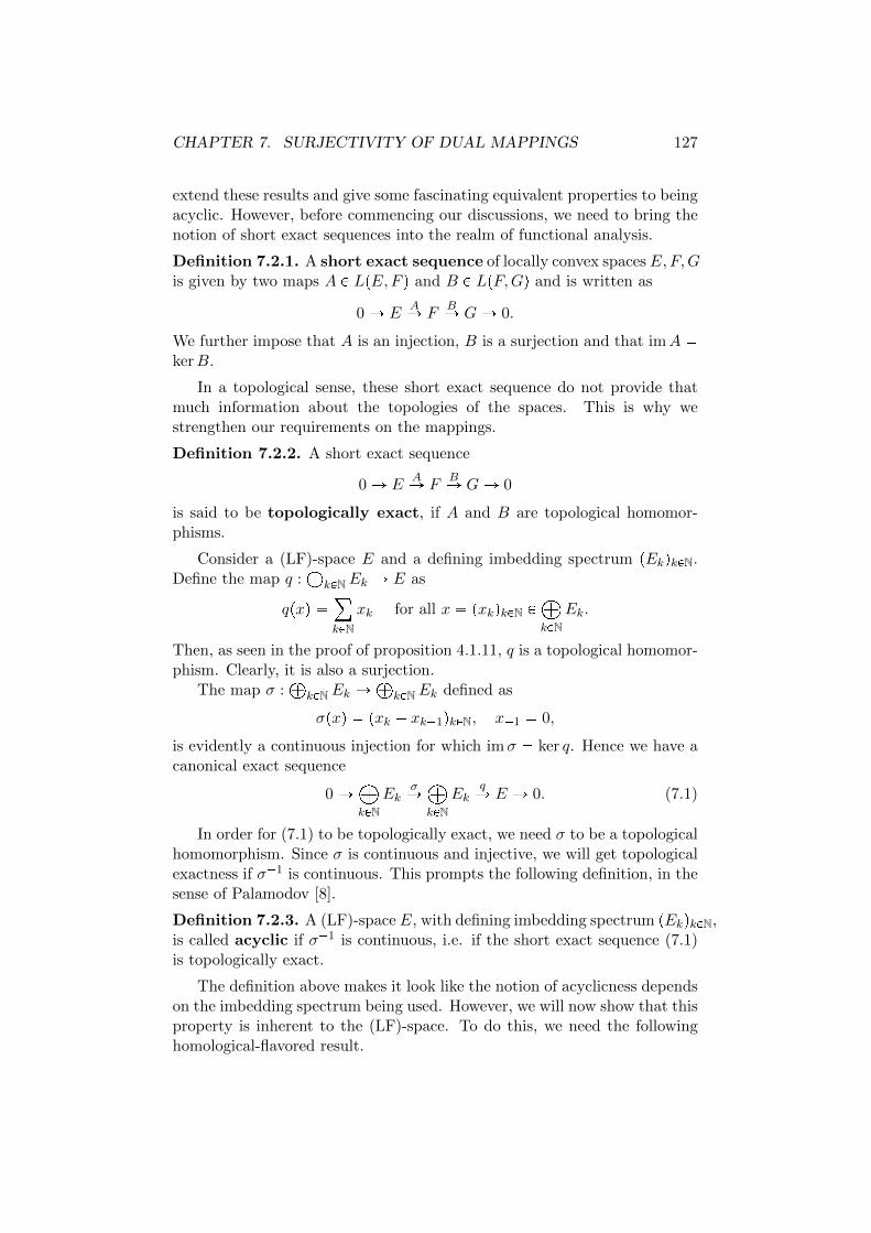
CHAPTER 7. SURJECTIVITY OF DUAL MAPPINGS 127
extend these results and give some fascinating equivalent properties to beingacyclic. However, before commencing our discussions, we need to bring thenotion of short exact sequences into the realm of functional analysis.
Definition 7.2.1. A short exact sequence of locally convex spaces E,F,Gis given by two maps A P LpE,F q and B P LpF,Gq and is written as
0 Ñ EAÑ F
BÑ GÑ 0.
We further impose that A is an injection, B is a surjection and that imA kerB.
In a topological sense, these short exact sequence do not provide thatmuch information about the topologies of the spaces. This is why westrengthen our requirements on the mappings.
Definition 7.2.2. A short exact sequence
0 Ñ EAÑ F
BÑ GÑ 0
is said to be topologically exact, if A and B are topological homomor-phisms.
Consider a (LF)-space E and a defining imbedding spectrum pEkqkPN.Define the map q :
ÀkPNEk Ñ E as
qpxq ¸kPN
xk for all x pxkqkPN PàkPN
Ek.
Then, as seen in the proof of proposition 4.1.11, q is a topological homomor-phism. Clearly, it is also a surjection.
The map σ :À
kPNEk ÑÀ
kPNEk defined as
σpxq pxk xk1qkPN, x1 0,
is evidently a continuous injection for which imσ ker q. Hence we have acanonical exact sequence
0 ÑàkPN
EkσÑ
àkPN
EkqÑ E Ñ 0. (7.1)
In order for (7.1) to be topologically exact, we need σ to be a topologicalhomomorphism. Since σ is continuous and injective, we will get topologicalexactness if σ1 is continuous. This prompts the following definition, in thesense of Palamodov [8].
Definition 7.2.3. A (LF)-space E, with defining imbedding spectrum pEkqkPN,is called acyclic if σ1 is continuous, i.e. if the short exact sequence (7.1)is topologically exact.
The definition above makes it look like the notion of acyclicness dependson the imbedding spectrum being used. However, we will now show that thisproperty is inherent to the (LF)-space. To do this, we need the followinghomological-flavored result.

CHAPTER 7. SURJECTIVITY OF DUAL MAPPINGS 128
Lemma 7.2.4. Let the following be a commutative diagram of topologicalvector spaces and linear maps with algebraically exact rows and columns
0 0 0 0 ÝÝÝÝÑ A
iÝÝÝÝÑ B
SÝÝÝÝÑ C ÝÝÝÝÑ 0
q
Q
T
0 ÝÝÝÝÑ D
hÝÝÝÝÑ E
PÝÝÝÝÑ F ÝÝÝÝÑ 0
k
j
G
pÝÝÝÝÑ H ÝÝÝÝÑ 0
0 0
Now assume that q, k and P are continuous, that h and j are open ontotheir range and that p and Q are open. Then i is open onto its range.
Proof. By their injectivity, we may assume that i, h, k and j are identicalimbeddings of subspaces. Let U be a zero neighborhood in A, then there isan absolutely convex zero neighborhood W E such that DX pW W q q1pUq. Then ppGXW q is a zero neighborhood in H, hence there is a zeroneighborhood V W in E such that H X P pV q ppG XW q. We claimthat A X QpV q U . Indeed, assume a Qv with a P A and v P V . ThenTPv SQv Sa 0, hence Pv P H X P pV q ppGXW q. So there existsw P G XW such that Pv pw. We have v w P W W and, because ofP pv wq 0, v w P D. Therefore
a Qv Qpv wq Qpwq Qpv wq qpv wq P U.
Since Q is open, this completes the proof of the lemma.
Proposition 7.2.5. Let E, with defining spectrum pEnqnPN, be an acyclic(LF)-space. If F and G are (LF)-spaces with defining spectra pFnqnPN,pGnqnPN and
0 Ñ GψÑ F
ϕÑ E Ñ 0
is a short exact sequence such that for every n there is an m with ψ1pFnq Gm, then the sequence is topologically exact.
Proof. Since ϕ is always open by the open mapping theorem 4.4.7, it sufficesto show that ψ is open onto its range.
It’s not hard to see that pϕFnqnPN is a defining spectrum for E, henceit is equivalent to pEnqnPN in the sense of corollary 4.5.9. Consequently, we
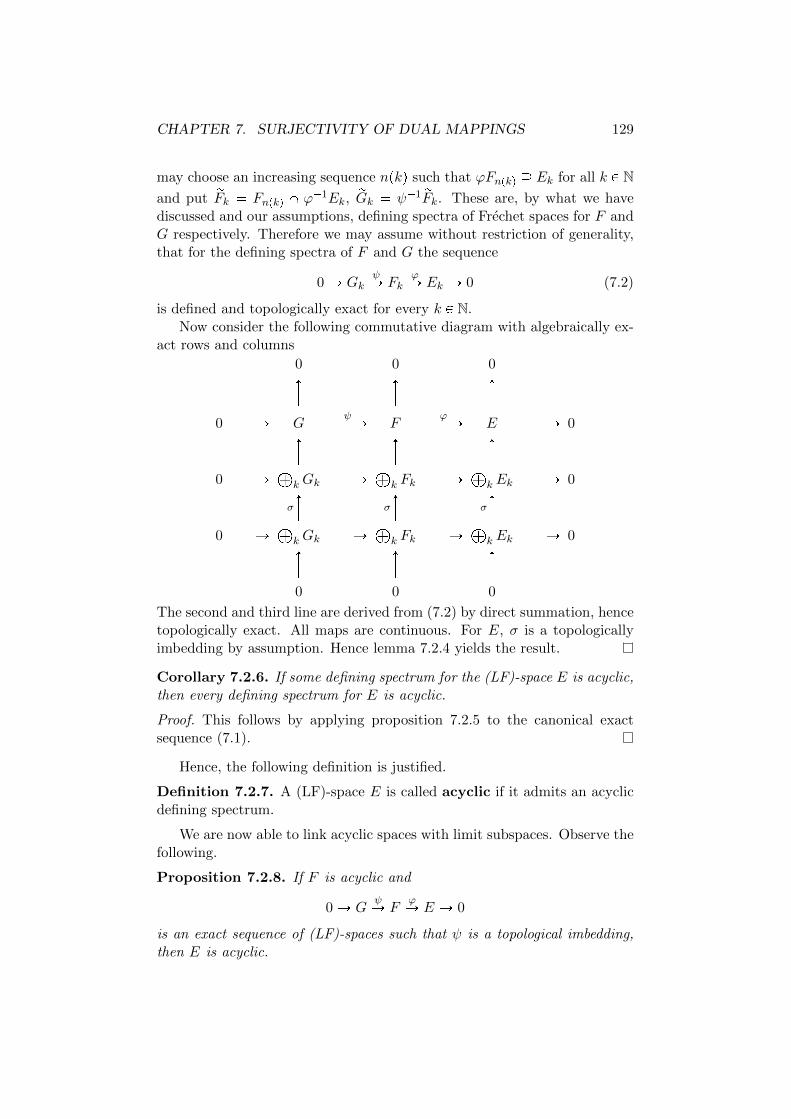
CHAPTER 7. SURJECTIVITY OF DUAL MAPPINGS 129
may choose an increasing sequence npkq such that ϕFnpkq Ek for all k P Nand put rFk Fnpkq X ϕ1Ek, rGk ψ1 rFk. These are, by what we havediscussed and our assumptions, defining spectra of Frechet spaces for F andG respectively. Therefore we may assume without restriction of generality,that for the defining spectra of F and G the sequence
0 Ñ GkψÑ Fk
ϕÑ Ek Ñ 0 (7.2)
is defined and topologically exact for every k P N.Now consider the following commutative diagram with algebraically ex-
act rows and columns
0 0 0 0 ÝÝÝÝÑ G
ψÝÝÝÝÑ F
ϕÝÝÝÝÑ E ÝÝÝÝÑ 0
0 ÝÝÝÝÑÀ
kGk ÝÝÝÝÑÀ
k Fk ÝÝÝÝÑÀ
k Ek ÝÝÝÝÑ 0
σ
σ
σ
0 ÝÝÝÝÑ
ÀkGk ÝÝÝÝÑ
Àk Fk ÝÝÝÝÑ
Àk Ek ÝÝÝÝÑ 0
0 0 0
The second and third line are derived from (7.2) by direct summation, hencetopologically exact. All maps are continuous. For E, σ is a topologicallyimbedding by assumption. Hence lemma 7.2.4 yields the result.
Corollary 7.2.6. If some defining spectrum for the (LF)-space E is acyclic,then every defining spectrum for E is acyclic.
Proof. This follows by applying proposition 7.2.5 to the canonical exactsequence (7.1).
Hence, the following definition is justified.
Definition 7.2.7. A (LF)-space E is called acyclic if it admits an acyclicdefining spectrum.
We are now able to link acyclic spaces with limit subspaces. Observe thefollowing.
Proposition 7.2.8. If F is acyclic and
0 Ñ GψÑ F
ϕÑ E Ñ 0
is an exact sequence of (LF)-spaces such that ψ is a topological imbedding,then E is acyclic.
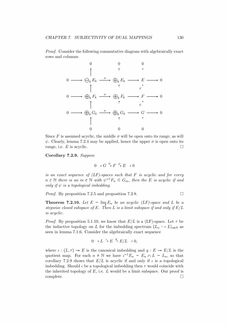
CHAPTER 7. SURJECTIVITY OF DUAL MAPPINGS 130
Proof. Consider the following commutative diagram with algebraically exactrows and columns
0 0 0 0 ÝÝÝÝÑ
Àk Ek
σÝÝÝÝÑ
Àk Ek ÝÝÝÝÑ E ÝÝÝÝÑ 0 ϕ
0 ÝÝÝÝÑ
Àk Fk
σÝÝÝÝÑ
Àk Fk ÝÝÝÝÑ F ÝÝÝÝÑ 0 ψ
0 ÝÝÝÝÑ
ÀkGk
σÝÝÝÝÑ
ÀkGk ÝÝÝÝÑ G ÝÝÝÝÑ 0
0 0 0
Since F is assumed acyclic, the middle σ will be open onto its range, as willψ. Clearly, lemma 7.2.4 may be applied, hence the upper σ is open onto itsrange, i.e. E is acyclic.
Corollary 7.2.9. Suppose
0 Ñ GψÑ F
ϕÑ E Ñ 0
is an exact sequence of (LF)-spaces such that F is acyclic and for everyn P N there is an m P N with ψ1Fn Gm, then the E is acyclic if andonly if ψ is a topological imbedding.
Proof. By proposition 7.2.5 and proposition 7.2.8.
Theorem 7.2.10. Let E limÝÑEn be an acyclic (LF)-space and L be astepwise closed subspace of E. Then L is a limit subspace if and only if ELis acyclic.
Proof. By proposition 5.1.10, we know that EL is a (LF)-space. Let τ bethe inductive topology on L for the imbedding spectrum pLn ãÑ LqnPN asseen in lemma 7.1.6. Consider the algebraically exact sequence
0 Ñ LιÑ E
qÑ ELÑ 0,
where ι : pL, τq Ñ E is the canonical imbedding and q : E Ñ EL is thequotient map. For each n P N we have ι1En En X L Ln, so thatcorollary 7.2.9 shows that EL is acyclic if and only if ι is a topologicalimbedding. Should ι be a topological imbedding then τ would coincide withthe inherited topology of E, i.e. L would be a limit subspace. Our proof iscomplete.
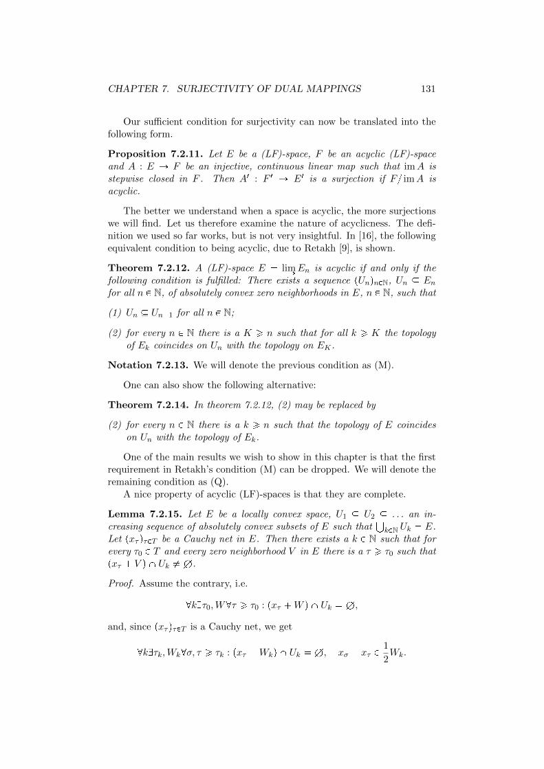
CHAPTER 7. SURJECTIVITY OF DUAL MAPPINGS 131
Our sufficient condition for surjectivity can now be translated into thefollowing form.
Proposition 7.2.11. Let E be a (LF)-space, F be an acyclic (LF)-spaceand A : E Ñ F be an injective, continuous linear map such that imA isstepwise closed in F . Then A1 : F 1 Ñ E1 is a surjection if F imA isacyclic.
The better we understand when a space is acyclic, the more surjectionswe will find. Let us therefore examine the nature of acyclicness. The defi-nition we used so far works, but is not very insightful. In [16], the followingequivalent condition to being acyclic, due to Retakh [9], is shown.
Theorem 7.2.12. A (LF)-space E limÝÑEn is acyclic if and only if thefollowing condition is fulfilled: There exists a sequence pUnqnPN, Un Enfor all n P N, of absolutely convex zero neighborhoods in E, n P N, such that
(1) Un Un1 for all n P N;
(2) for every n P N there is a K ¥ n such that for all k ¥ K the topologyof Ek coincides on Un with the topology on EK .
Notation 7.2.13. We will denote the previous condition as (M).
One can also show the following alternative:
Theorem 7.2.14. In theorem 7.2.12, (2) may be replaced by
(2) for every n P N there is a k ¥ n such that the topology of E coincideson Un with the topology of Ek.
One of the main results we wish to show in this chapter is that the firstrequirement in Retakh’s condition (M) can be dropped. We will denote theremaining condition as (Q).
A nice property of acyclic (LF)-spaces is that they are complete.
Lemma 7.2.15. Let E be a locally convex space, U1 U2 . . . an in-creasing sequence of absolutely convex subsets of E such that
kPN Uk E.
Let pxτ qτPT be a Cauchy net in E. Then there exists a k P N such that forevery τ0 P T and every zero neighborhood V in E there is a τ ¥ τ0 such thatpxτ V q X Uk H.
Proof. Assume the contrary, i.e.
@kDτ0,W@τ ¥ τ0 : pxτ W q X Uk H,
and, since pxτ qτPT is a Cauchy net, we get
@kDτk,Wk@σ, τ ¥ τk : pxτ Wkq X Uk H, xσ xτ P1
2Wk.

CHAPTER 7. SURJECTIVITY OF DUAL MAPPINGS 132
We may assume Wk1 Wk, Wk P U0pEq for all k P N. Now put Wpnqk :
WkXUn. Then Wpnqk is a zero neighborhood in Un for the topology induced
by E. We put
Vk : Γ
1
2W
p1q1 Y Y
1
2W
pk1qk1 YWk
and claim that pxτ Vkq X
12Uk H for every τ ¥ τk.
Assume that this is not the case. Then there is a τ ¥ τk and z Ppxτ Vkq X
12Uk. Hence we have
z xτ k
i1
αixi P1
2Uk
with xi PWpiqi , i 1, . . . , k 1, xk PWk and
°ki1 |αi| ¤ 1. Therefore
z k1
i1
αixi xτ αkxk P Uk X pxτ Wkq,
contradicting the choice of Wk.Now put
U : Γ
8¤k1
1
2W
pkqk
,
then U P U0pEq and U Vk for all k P N, since for m ¥ k we have
Wpmqm W
pmqk Wk Vk. Now choose τ0 P T such that xσ xτ P U for
σ, τ ¥ τ0 and σk ¥ τ0, σk ¥ τk. Then
xτ0 xσk pxτ0 xσkq P xσk U xσk Vk.
Hence 2xτ0 R Uk for all k P N, contradictingkPN Uk E.
Proposition 7.2.16. An acyclic (LF)-space E is complete.
Proof. Let pxτ qτPT be a Cauchy net in E. Take a sequence pUnqnPN givenby theorem 7.2.12. For the purpose of our proof, we may assume thatnPN Un E, since a Cauchy net is bounded, hence contained in some
dilation of U1 (and thus in the same dilation of every Un). Then accordingto lemma 7.2.15 there is a n P N such that for every τ P T and V P U0pEqthere is a σ ¥ τ and xτ,V P pxσ V q X Un. Then pxτ,V qτPT,V is a Cauchynet in Un for the topology induced by E. Indeed, let U be some absolutelyconvex zero neighborhood of E, τ0 P T be such that xσ xτ P
12U for each
τ, σ ¥ τ0 and let W P U0pEq such that W W 12U . Then we have for
each τ, σ ¥ τ0 and W 1,W 2 W :
xσ,W 1 xτ,W 2 P p1
2U W 1 W 2q X Un p
1
2U W W q X Un U X Un.
CHAPTER 7. SURJECTIVITY OF DUAL MAPPINGS 133
Consequently, because of theorem 7.2.14, there is a k ¥ n such that pxτ,V qτPT,Vis a Cauchy net in Un for the topology induced by Ek. Hence it convergesto some x P Un. Then clearly pxτ qτPT will converge to x as well.
7.3 Retractive (LF)-spaces
In this paragraph, we discuss some regularity conditions on (LF)-spaces.Even more, we will show that they are all equivalent to being acyclic. Theresults that will be presented are based on the article [17] by Wengenroth.We start by introducing some of the equivalent notions.
Definition 7.3.1. Let pE, tq limÝÑEn be the inductive limit of the imbed-ding spectrum pjn : En Ñ EqnPN. The defining spectrum pEnqnPN is said tobe
(1) regular if every bounded set B in E is contained and bounded in oneof the steps;
(2) sequentially retractive if every null sequence in E converges to zeroin some step;
(3) boundedly retractive if for every bounded set B in E there is a n P Nsuch that B is contained in En and the topology of En coincides with ton B;
(4) (sequentially) compactly regular if every (sequentially) compactsubset of the inductive limit is (sequentially) compact in some step.
In the case of (LF)-spaces, the above definitions are inherent to the spaceitself.
Lemma 7.3.2. If E is a (LF)-space and pEnqnPN and pFnqnPN are bothdefining spectra for E, then pEnqnPN is regular or sequentially retractive orboundedly retractive or (sequentially) compactly regular if and only if pFnqnPNhas the corresponding property.
Proof. This follows directly from corollary 4.5.9.
Remark 7.3.3. Because of lemma 7.3.2, we will say that a (LF)-space isregular, sequentially retractive, boundedly retractive or (sequentially) com-pactly regular if one of its defining spectra has the corresponding property.

CHAPTER 7. SURJECTIVITY OF DUAL MAPPINGS 134
Lemma 7.3.4. The following hierarchy concerning regularity holds for a(LF)-space E limÝÑEn:
1. if E is boundedly retractive, then E is (sequentially) compactly regular;
2. if E is (sequentially) compactly regular, then E is sequentially retrac-tive;
3. if E is boundedly retractive, then E is sequentially retractive.
Proof. (1) Since every (sequentially) compact set is bounded, by properties2.2.22(c) and (d), this follows immediately.
(2) Let pxnqnPN be a null sequence in E and put S t0u Y txn : n P Nu.Then S is (sequentially) compact in E. Hence it is contained in some stepEm and it is (sequentially) compact there. Since sequential compactness andcompactness are equivalent in a metric space (in particular a Frechet space)by lemma 1.3.2, we see that S is sequentially compact in Em. Consequently,pxnqnPN has a convergent infinite subsequence in Em, and by the continuity ofthe imbedding jm : Em ãÑ E, this subsequence necessarily converges to zero.This already implies that should pxnqnPN converge in Em, it must convergeto 0. Now suppose that it does not converge in Em, then we can find aU P U0pEmq and an infinite subsequence pxnkqkPN of pxnqnPN not containedin U . Consider S 1 t0u Y txnk : k P Nu. Since pxnkqkPN converges to zeroin E, S 1 is closed in E and thus also in Em. Since S 1 S, we see that S 1is sequentially compact in Em. This implies that pxnkqkPN has a convergentsubsequence converging to 0. But this subsequence would be contained inU starting from a certain step, contradicting the choice of pxnkqkPN. Thus,we may conclude that pxnqnPN converges to zero in Em.
(3) Follows from (1) and (2).
Our result on the completeness of acyclic (LF)-spaces already shows thatit satisfies some of the regularity conditions.
Proposition 7.3.5. An acyclic (LF)-space E is boundedly retractive, inparticular sequentially retractive.
Proof. By proposition 7.2.16, E is complete. Take some defining spectrumpEnqnPN for E. Now let B be a bounded set of E. Since ΓB is also bounded,we may assume that B is closed and absolutely convex. Since E is complete,B will be complete as well, so that by corollary 2.2.32, B is a Banachdisk. This means that EB is a Banach space, which enables us to useGrothendieck’s factorization theorem 4.5.8 to find an m P N, so that EB(in particular B) is contained in Em and such that there is an injectivev P LpEB, Emq. Then B will also be bounded in Em, so that we mayconclude that E is regular.
Now every bounded set B is contained in some Em and bounded there,hence contained in some λUµ as in theorem 7.2.12. Then theorem 7.2.14
CHAPTER 7. SURJECTIVITY OF DUAL MAPPINGS 135
implies that the topologies of E and Ek coincide on B, for some k ¥ m,which implies bounded retractiveness.
Thus, by theorem 7.2.12, (LF)-spaces satisfying (M) are boundedly re-tractive, so in particular they are sequentially retractive. To show the re-verse, we start by proving that sequential retractiveness implies (Q).
Proposition 7.3.6. Every sequentially retractive (LF)-space E limÝÑEnsatisfies (Q).
Proof. It suffices to show that for every n P N there is a Un P U0pEnq and aK ¡ n such that for all k ¥ K, the topologies of Ek and E have the sameconvergent sequences in Un. By the definition of an imbedding spectrum,we already know that a sequence converging for the topology in Ek willalso converge in El, for each l ¥ k, and in E. Hence, if we can show thatsequences, contained in Un, converging in E, also converge in some EK ,K P N¡n, we are finished.
Fix a n P N and let pVkqkPN be a decreasing basis of absolutely convex,closed zero neighborhoods in En. Suppose that for every k P N there is asequence pxk,lqlPN in Vk that converges to some xk P Vk in E but not inEnk. Next, consider the net pyk,lqpk,lqPN2 , with yk,l : xk,l xk. We willshow that this net converges to 0 in E. Note, by the choice of the Vk’s,that for each l P N, the sequence pxk,lqkPN converges to 0 in En, and thus E,uniformly. This means that for each U P U0pEq there is a K P N such thatfor each l P N, k ¥ K, we have xk,l P U . Since pxkqkPN also converges to 0in E, we can conclude that the net pyk,lqpk,lqPN2 converges to 0 in E. ButE is sequentially retractive by hypothesis, hence the net converges in somestep Enk0 . This implies that the sequence pyk0,lqlPN also converges to 0 inEnk0 , a contradiction. Consequently, by putting Un : Vk0 , we see that(Q) holds for E.
Next, we wish to show that (Q) implies (M), i.e. the first condition of(M) can be dropped to get an acyclic space. In order to do this, we needthe following result.
Lemma 7.3.7. Let E be a vector space and S, T two locally convex topolo-gies on E. Let A be an absolutely convex subset of E and assume that thereis an absolutely convex zero neighborhood U in pE,Sq such that S|UXA iscoarser than T |UXA. Then S|A is coarser than T |A.
Proof. Take an arbitrary absolutely convex zero neighborhood V in pE,Sq.Since V X 1
2U is a zero neighborhood in pE,Sq, there is an absolutely convexzero neighborhood W in pE, T q such that W X A X U V X 1
2U . Nowsuppose that x P W X A but x R U . Then there is a n P N with 1
2nx P U ,but 1
2n1x R U . Since W and A are absolutely convex this implies 12nx P
W XAXU 12U . Therefore, 1
2n1x P U , which contradicts the choice of n.From this we can conclude that W XA V , and our proof is complete.
CHAPTER 7. SURJECTIVITY OF DUAL MAPPINGS 136
Proposition 7.3.8. A (LF)-space E limÝÑpEn, Tnq that satisfies (Q) alsosatisfies (M).
Proof. Let pUnqnPN be given by (Q). First of all, note that if (M) holds fora defining spectrum which is a subsequence of the given one, then (M) willalso holds for the original defining spectrum, by corollary 7.2.6 and theorem7.2.12. So, we may assume that for every n, k P N already Tn1|Un Tnk|Unholds.
By the coincidence of T2 and T3 on U1, there is a V3 P U0pE3q such that2V3XU1
12U2. Define rU2 U1p
12U2XV3q, which is an absolutely convex
zero neighborhood in E2 containing U1.By lemma 7.3.7, in order to show that T3|rU2
T3k|rU2for every k P N,
it is enough to show the coincidence of the topologies on rU2 X V3. But
rU2 X V3 pU1 p1
2U2 X V3qq X V3 pU1 X 2V3q p
1
2U2 X V3q
1
2U2
1
2U2 U2,
so that the topologies coincide on U2 (and thus rU2 X V3) by assumption.Hence our claim is valid. Proceeding by induction yields that the inductivespectrum satisfies (M).
Corollary 7.3.9. Sequentially retractive (LF)-spaces are acyclic.
Proof. By propositions 7.3.6, 7.3.8 and theorem 7.2.12.
Corollary 7.3.10. Sequentially retractive (LF)-spaces are complete.
We can now summarize all equivalent conditions to being acylic in thefollow theorem.
Theorem 7.3.11. For a (LF)-space E the following conditions are equiva-lent:
(1) E is acyclic;
(2) E satisfies (M);
(3) E satisfies (Q);
(4) E is boundedly retractive;
(5) E is compactly regular;
(6) E is sequentially compactly regular;
(7) E is sequentially retractive.
CHAPTER 7. SURJECTIVITY OF DUAL MAPPINGS 137
Proof. p1q ô p2q follows from theorem 7.2.12, while p2q ô p3q follows fromproposition 7.3.8. p1q ñ p4q was shown in proposition 7.3.5 and we alsohave p4q ñ p5q, p4q ñ p6q, p5q ñ p7q by lemma 7.3.4. Finally, p7q ñ p1q isstated in corollary 7.3.9.
Our understanding of acyclicness, and thus our search for surjections,has become much more intuitive. To illustrate the strength of theorem7.3.11, and to give examples of acyclic (LF)-spaces, let us take a look atstrict (LF)-spaces.
Corollary 7.3.12. Strict (LF)-spaces are acyclic. In particular, they arecomplete.
Proof. Let E limÝÑEn be a strict (LF)-space. We will show that E issequentially retractive, hence acyclic by theorem 7.3.11 and complete bycorollary 7.3.10.
First of all, note that, due to corollary 4.5.4, should a sequence convergeto 0 in E and be contained in any of its steps En, it would also converge to0 in En. Hence, if E were not to be sequentially retractive, we would find asequence, converging to 0 in E, not contained in any of its steps. By goingto a subsequence, we would find a sequence pxnqnPN, converging to 0 in E,such that xn R En for each n P N.
Take an arbitrary U1 P U0pE1q. Then, using lemma 4.5.3, we can finda U2 P U0pE2q such that U1 U2 X E2 and x1 R U2. By applying lemma4.5.3 twice and taking the intersection, we find a U3 P U0pE3q such thatx1, x2 R U3. In general, using induction, we find a Un P U0pEnq such thatx1, . . . , xn1 R Un, for each n P N. Now put U
8n1 Un. Since U X En
Un, U is a zero neighborhood of E by properties 4.1.9(b). Hence there is aN P N such that for each m ¥ N , xm P U . But this is clearly in contradictionto the construction of U . Hence, our proof is complete.
7.4 Inductive limits of Frechet-Montel spaces
Let us now impose more structure on our imbedding spectra, in the hope ofgetting easier characterizations of acyclicness. More specific, let us consider(LF)-space whose steps are Frechet-Montel spaces, such as the space of testfunctions DpΩq. For these spaces, we will show that one can add more simpleforms of regularity and even completeness to theorem 7.3.11. To do this, weintroduce a weakened version of (Q).
Definition 7.4.1. An inductive limit E limÝÑEn is said to satisfy (wQ)if there is a sequence pUnqnPN such that, for each n P N, Un P U0pEnq andthere is a m ¡ n so that for each k ¥ m and each W P U0pEmq there is aV P U0pEkq and S ¡ 0 with V X Un SW .
CHAPTER 7. SURJECTIVITY OF DUAL MAPPINGS 138
Remark 7.4.2. Note that without the factor S in (wQ), the condition wouldmean that Ek and Em induce the same topology in Un, i.e. the condition(Q).
As can easily be seen, (wQ) is equivalent to the following inequalities,which are appropriate for calculations in concrete cases:
Lemma 7.4.3. Let E limÝÑEn be a (LF)-space and let p‖‖n,lqlPN be afundamental system of seminorms in En for each n P N. Then E satisfies(wQ) if and only if the following holds
@nDm ¡ n,N P N@k ¡ m,M P NDK P N, S ¡ 0@x P En
‖x‖m,M ¤ S‖x‖k,K ‖x‖n,N
.
In [1], another equivalent condition to (wQ) was shown.
Lemma 7.4.4. A (LF)-space E limÝÑEn satisfies (wQ) if and only if forevery n P N there is a Un P U0pEnq and a m ¡ n such that for each k ¥ m,Ek and Em have the same bounded sets in Un.
Proof. Suppose first that E satisfies (wQ). Let, for an arbitrary n P N, Unand m be given as in the definition of (wQ). First note that for every k ¥ m,all bounded set in Em are also bounded in Ek. Now take a k ¥ m and let Bbe a bounded set in Ek, contained in Un. For any W P U0pEmq, let V and Sbe given by (wQ). Then there is a λ ¡ 0 such that B λpV XUnq λSW .Hence B is also bounded in Ek, and our first implication is proven.
Now suppose that E satisfies the condition concerning the bounded sets.For n P N, let Un and m ¡ n be given as in the condition. Presume, inorder to get a contradiction, that for some k ¥ m and W P U0pEmq, we havethat for each V P U0pEkq and S ¡ 0 that V X Un is not contained in SW .Let pVµqµPN be a descending zero neighborhood basis in Ek and choose foreach µ P N a xµ P pVµ X UnqzµW . Then txµ : µ P Nu is bounded in Ek andcontained in Un, but it is not bounded in Em, a contradiction.
Next, we introduce two notions that come close to regularity, yet areweaker in one aspect.
Definition 7.4.5. Let E limÝÑEn be an inductive limit.
(1) E is called α-regular if every bounded set is contained (but not neces-sarily bounded) in some step.
(2) E is called β-regular if every bounded set which is contained in a stepis also bounded in some step.
Proposition 7.4.6. A (LF)-space E limÝÑEn which is either α- or β-regular satisfies (wQ).
CHAPTER 7. SURJECTIVITY OF DUAL MAPPINGS 139
Proof. Suppose first that E is α-regular and fix n P N. Then there is an
absolutely convex zero neighborhood Un and m ¡ n such that UEn Em.
Indeed, let pVkqkPN be a decreasing, absolutely convex zero neighborhoodbasis of En and assume that for every k P N there is a xk in the E-closureof Vk but not contained in Ek. Given a W P U0pEq, there is a k P Nwith V
Ek W . This means that xk Ñ 0 in E without being contained
in any step, a contradiction. Let now k ¡ m and B Un bounded in
Ek. Then, by corollary 2.2.32, D ΓpBqEk
is a Banach disk contained inEm. The identity map ED ãÑ Em has a closed graph since both spaces arecontinuously included in Ek. Hence, the closed graph theorem 4.4.8 impliesthat this identity map is continuous and therefore B is bounded in Em.Consequently, using lemma 7.4.4, E satisfies (wQ).
Let now E be β-regular. Again, fix a n P N and choose a decreasing basisof zero neighborhoods pVkqkPN in En. Assume that for every k P N there isa Bk Vk which is bounded in E but not bounded in Ek. Then the unionB
kPNBk is contained in En and again bounded in E. Indeed, if W is
a zero neighborhood in E, there is a k P N with Vk W and a 0 λ ¤ 1with λ
1¤j k Bj W . Hence, λB W . Now β-regularity implies that B
is bounded in some step Ek, a contradiction since Bk B is unbounded inEk. Let k P N be such that Ek and E share the same bounded sets in Vk.For each m ¥ k, all bounded sets in Em are also bounded in E, hence Ekand Em have the same bounded sets in Vk. Lemma 7.4.4 then implies thatE satisfies (wQ).
The previous proposition now instantly allows us to refine theorem 7.3.11for inductive limits of Frechet-Montel spaces.
Theorem 7.4.7. Let E limÝÑEn be a (LF)-spaces where each step is aFrechet-Montel space. The following conditions are equivalent:
(1) E is acyclic;
(2) E is complete;
(3) E is regular;
(4) E is α-regular;
(5) E is β-regular;
(6) E satisfies (wQ).
Proof. p1q ñ p2q was show in lemma 7.2.15. p2q ñ p3q follows from theproof of proposition 7.3.5 by noting that in order to show regularity, weonly needed completeness. The implications p3q ñ p4q and p3q ñ p5q aretrivial, while p4q ñ p6q and p5q ñ p6q were shown in proposition 7.4.6.Hence we are left with showing p6q ñ p1q.

CHAPTER 7. SURJECTIVITY OF DUAL MAPPINGS 140
Suppose E satisfies (wQ). Using lemma 7.4.4, we find a sequence pUnqnPNof zero neighborhoods of the steps in which almost all step topologies havethe same bounded sets. Let n P N be arbitrary and m ¡ n such that alltopologies of Ek, k ¥ m, have the same bounded sets in Un. Fix a k ¥ mand let pxlqlPN be a sequence in Un which converges to 0 in the topologyof Ek. This sequence is then bounded and hence relatively compact in thetopology of Em, since it is a Montel space. Analogously as in the proofof lemma 7.3.4(2), we may conclude that the sequence tends to 0 also inEm. Thus, the topologies of Ek and Em coincide in Un, i.e. (Q) is satisfied.Theorem 7.3.11 now implies that E is acyclic.
This allows us to find examples of acyclic (LF)-spaces that are not nec-essarily strict.
Corollary 7.4.8. The inductive limit of a weakly compact imbedding spec-trum of normed Montel spaces is acyclic.
Proof. This follows from proposition 5.3.7.
Let us now translate some of these properties in order to find easilyverifiable means to detect the acyclicness of quotients, i.e. to identify sur-jections.
Lemma 7.4.9. For an inductive limit E limÝÑEn, E is α-regular if andonly if each weak null sequence is contained in some step.
Proof. A weak null sequence is weakly bounded, hence bounded in E byMackey’s theorem 3.2.4, so that α-regularity implies the property above. Toshow the inverse implication, one can use a similar technique as in the proofof proposition 7.3.6.
Theorem 7.4.10. Let A : E Ñ F be an injective, continuous linear mapfrom a (LF)-space E to an acyclic inductive limit F limÝÑFn of Frechet-Schwartz spaces Fn such that imA is stepwise closed. Let p‖‖n,lqlPN bea fundamental system of seminorms in Fn for each n P N. Then A1 issurjective if one of the following conditions is satisfied:
1. For every sequence pykqkPN in F converging pointwise to 0 on kerA1
there is a n P N and a sequence pxkqkPN in E such that ykApxkq P Fnfor each k P N.
2.
@nDm ¡ n,N P N@k ¡ m,M P NDK P N, S ¡ 0
@x P En@y1 P A1pFkq@y2 P A
1pFnq
infyPA1pFmq
‖xAy‖m,M ¤ S‖xAy1‖k,K ‖xAy2‖n,N
.
CHAPTER 7. SURJECTIVITY OF DUAL MAPPINGS 141
Proof. By propositions 4.3.4 and 5.1.7, the quotient of each Frechet-Schwartzspace will again be Frechet-Schwartz, hence Montel (properties 4.3.12(b)).Hence, F imA will be an inductive limit of Frechet-Montel spaces. There-fore, by proposition 7.2.11, if F imA satisfies one of the equivalent condi-tions in theorem 7.4.7, A1 will be surjective.
(1) This follows from lemma 7.4.9.(2) Is a translation of lemma 7.4.3.
We refer to the article [4] by Frerick and Wengenroth, where theorem7.4.10 is applied to find sufficient conditions for the solvability of the con-volution problem.

Conclusion
A continuous linear map A between two locally convex spaces E and F is asurjection if and only if the image of A is closed and dense in F . Since therichness of the theory of locally convex spaces greatly stems from the inter-play between a space and its dual, it is to be expected that the surjectivityof A could be translated in terms of the duals E1, F 1 and the transpose mapA1. In theorem 3.4.12, we saw that A is a surjection if and only if A1 isinjective and a weak homomorphism. Although these conditions, especiallythe latter, might be difficult to verify, it does guide us to more easy verifiablesolutions in less general spaces.
Knowing which functions are homomorphisms thus helps us find surjec-tions. This is why a more general version of the open mapping theoremwas in order. In chapter 4, see theorem 4.4.7, we saw that a continuouslinear surjection between a webbed space and an ultra-bornological space isautomatically open. Examples of such spaces are the Frechet spaces, (LF)-spaces and (DFS)-spaces. Starting from chapter 6, we would then applysaid theorem to find surjections linked to these respective spaces.
In theorem 6.1.5, we saw that a continuous linear map A between aMackey webbed space E and an ultra-bornological space F , such that E kerAis complete and imA is Mackey, is surjective if and only if A1 is injectiveand imA1 is weakly closed. Since Hausdorff quotients of Frechet spaces,(DFS)-spaces and (PLS)-spaces are consistently complete, these spaces canalways be used on the left-hand side of the theorem. On the right-handside, metrizable ultra-bornological spaces are applicable. In particular, weget a characterization of surjections between Frechet spaces. These results,including a refinement in the form of theorem 6.2.8, were then demonstratedin the form of two applications: a classical result by E. Borel and a char-acterization of the solvability of linear partial differential equations withinfinitely differentiable coefficients.
In chapter 7, we looked at the problem from another perspective andwondered when the transposed map of a continuous linear map A : E Ñ Fis a surjection. In lemma 7.1.1, we saw that it suffices for A to be an injectivehomomorphism for this to be true. As stated above, this is easily verifiableif we could apply the open mapping theorem. But then E needs to bewebbed and imA needs to be ultra-bornological. In the case where E and F
142

CHAPTER 7. SURJECTIVITY OF DUAL MAPPINGS 143
are (LF)-spaces, this is true if imA is again a (LF)-space. Theorem 7.2.10showed that this question is linked with the notion of acyclic (LF)-spaces,which are exactly the sequentially retractive (LF)-spaces, as seen in theorem7.3.11. This allowed us to find some verifiable conditions that are sufficientfor the dual map to be surjective.
Indication of the usedsources
In this paragraph, we give a short overview of the sources we used and whichresults were original. We will do this by chapter, so that the reader mayeasily find additional information if necessary.
The first chapter was mainly written by heart, and any text dealing withthe basics of topology and functional analysis should contain the results thatwe have dealt with. If a conclusion was not explained, then a proof canalways be found in either [7] or [15].
In chapter 2 we made our own construction, yet we were essentiallyinspired by chapter 22 of [7]. Some results from [15] were also establishedhere. Starting from Milman’s theorem and the application following it, wefollowed the logic found in [12], which was in its turn inspired by [5].
In chapter 3, we primarily followed the construction as in [7], with someresults from [15] added in. The inspiration for the Mackey spaces and theirlater application came from [6] and [13]. Some inspiration was also takenfrom [10].
Chapter 4 is again an amalgam of results and structures from [7] and[15], while the generalized open mapping theorem comes from [18], but asimilar proof can also be found in [7].
In chapter 5 we exclusively followed the structure of chapter 25 in [7].The surjectivity result in chapter 6 is an original extension of a result
due to S. Banach. We primarily extended the logic found in [15] using theproperties of Mackey spaces. This extends the theorem to more spaces thanjust the Frechet spaces, especially on the left-hand side. The remainder ofthe chapter deals with surjectivity between Frechet spaces, as is done in [15].
Chapter 7 was inspired by several articles on the notion of acyclicness.First, the logic that finds a sufficient condition for the dual to be onto isoriginal, and was inspired by the article [4]. The connection between thelimit subspaces and the acyclic quotients, as well as the equivalent regularityconditions to acyclicness, came form [17]. We used the article [16] to estab-lish some basic results of the acyclic (LF)-spaces and [9] for an equivalentdefinition. A result from [1] was also used.
144
Appendix A
Nederlandstaligesamenvatting
In deze master thesis gaan we na onder welke voorwaarden een afbeeldingA tussen twee lokaal convexe ruimten E en F een surjectie is. Opdat ditwaar zou zijn, is het nodig en voldoende dat het beeld van A gesloten endicht is in F . Eerder dan dit probleem te bestuderen in specifieke gevallen,opteerden we ervoor om dit in een algemeen kader te doen. Om dergelijkestudie mogelijk te maken, is er een grondige kennis omtrent de gebruikteruimten nodig. Daarom wordt een groot deel van dit werk besteed aan eenalgemeen overzicht van de lokaal convexe ruimten.
We starten in hoofdstuk 1 met een kort overzicht van enkele begrippenen resultaten waarvan we uitgaan dat de lezer ermee vertrouwd is. Onder-werpen die behandeld worden zijn onder andere algemene topologie, topol-ogische vectorruimten, metriek en de Baire categorien. Dit hoofdstuk iseerder bedoeld als een referentielijst, die de lezer doorheen het vervolg kanraadplegen daar waar nodig.
In hoofdstuk 2 voeren we de lokaal convexe ruimten in, dewelke hetkader vormen waarin we doorheen deze thesis zullen werken. Lokaal convexeruimten kan men zien als vectorruimten waarop we een continue familievan seminormen definieren. Dit laat ons toe begrippen zoals convergentieen begrensdheid analoog te representeren zoals bij genormeerde ruimten.Het tweede hoofdstuk heeft voornamelijk tot doel de lokaal convexe ruimtenzodanig te verkennen zodat we deze in het vervolg zonder veel moeite kunnentoepassen. Toch bespreken we hier reeds een toepassing, met name eenfixpuntstelling van S. Kakutani.
Voortbouwend op de lokaal convexe ruimten, behandelen we in hoofdstuk3 hun dualen. Specifiek bekijken we op welke wijze we deze van een topolo-gie kunnen voorzien zodat deze eveneens lokaal convex zijn. Doorheen dithoofdstuk zullen we een bijzondere verbintenis ontdekken tussen een lokaalconvexe ruimte en zijn duale, waarbij de ene de andere beınvloedt. Tevens
145

APPENDIX A. NEDERLANDSTALIGE SAMENVATTING 146
tonen we reeds onze eerste karakterisatie van surjectiviteit aan, die stelt dateen continue lineare afbeelding A tussen twee lokaal convexe ruimten sur-jectief is als en slechts als zijn getransponeerde afbeelding een injectief zwakhomomorfisme is.
Na een grondige studie van de lokaal convexe ruimten, bekijken we inhoofdstuk 4 hoe we nieuwe ruimten uit andere kunnen opbouwen. Dit doenwe aan de hand van de projectieve en inductieve topologie. Hierdoor zullenwe een veelheid aan nieuwe ruimten introduceren, zoals de bornologischeruimten en de Schwartz ruimten. Het belangrijkste resultaat uit dit hoofd-stuk zal een algemenere versie van de open afbeeldingsstelling zijn, een zeerbelangrijk resultaat in de zoektocht naar surjecties.
In hoodstuk 5 richten we ons op een specifieke studie van de Frechetruimten en hun dualen. Hierbij vinden we enkele sterke eigenschappen dieons toelaten om in hoofdstuk 6 surjecties tussen Frechet ruimten te karak-teriseren. Meer nog, we bewijzen een veralgemening van een resultaat doorS. Banach die ondermeer de Frechet ruimten bevat. Specifiek tonen we aandat een afbeelding tussen bepaalde ruimten surjectief is als en slechts alshaar duale injectief is en een zwak gesloten beeld heeft. Op basis van ditresultaat behandelen we daarna twee toepassingen: een klassieke stellingdoor E. Borrel en een karakterisatie van de oplosbaarheid van partiele dif-ferentiaalvergelijkingen.
Tot slot, in hoofdstuk 7, draaien we het probleem om en vragen we onsaf wanneer de duale afbeelding surjectief is. Dit zal het geval zijn wanneerde originele afbeelding een injectief homomorfisme is. Vervolgens bekijkenwe dit probleem in het geval van (LF)-ruimten, waar we zullen zien datde oplossing bij een uitgebreide kennis van de zogenaamde acyclische (LF)-ruimten ligt. Daaraan zal het resterende deel van het zevende hoofdstukgewijd zijn.
Appendix B
Distributions
B.1 The distribution space D1pΩq
In this appendix we aim to give a brief overview of the results, concerningdistributions, that are used in our main text. In particular, we will bediscussing the space of distributions D1pΩq that is the dual of the (LF)-spaceof test functions DpΩq for some open set Ω of Rn, as examined in example4.5.10. It is not our intention to give a full treatise on this subject, or evento prove all results that will be listed, but rather to give some intuition andto give some facts. We expect the reader to be somewhat familiar with thesubject, hence this appendix could be used as a cheat sheet. Our discussionwill be based on Treves book [15].
Using corollary 2.2.9 and proposition 4.1.10, we may now characterizethe distributions.
Theorem B.1.1. Let f : DpΩq Ñ C be a linear functional. Then f P D1pΩqif and only if for every compact K Ω, there are M MK ¡ 0 andN Nk P N such that
|xf, φy| ¤M ‖φ‖N , for all φ P DpΩq, suppφ K. (B.1)
Definition B.1.2. If there is a N , independent of K, such that (B.1) holds,for constant M MK , then the distribution is said to be of order N .Otherwise, the distribution is said to have infinite order on Ω.
Let us look at some examples of distributions.
Examples B.1.3. (1) The Dirac delta distribution δ is defined as
xδ, φy φp0q, for all φ P DpRnq.
(2) The Heaviside function H is the distribution, on the real line, definedby
xH,φy
» 8
0φpxqdx, for all φ P DpRq.
147
APPENDIX B. DISTRIBUTIONS 148
(3) For every f P L1locpΩq we define the unique distribution
xf, φy
»Ωfpxqφpxqdx, for all φ P DpΩq.
These are called regular distributions.
Given a f P D1pΩq, we may always restrict f to an open subset ω Ω,that is, we can view f P D1pωq. Two distributions f, g P D1pΩq are said tobe equal on ω Ω if
xf, φy xg, φy, @φ P Dpωq.
We writef g on ω.
The following can now be shown.
Lemma B.1.4. The union of all open sets of Ω on which f P D1pΩq vanishesis also an open subset of Ω on which f vanishes.
Proof. This is a corollary of the so called ’Sewing lemma’ (see [15], theorem24.1 on page 253).
The following definition is now well-defined.
Definition B.1.5. Let f P D1pΩq. The complement of the largest opensubset of Ω on which f vanished is called the support of f and is denotedby supp f .
Consider now the Frechet space C8pΩq of all C8-functions on Ω. ThenDpΩq can be continuously imbedded in C8pΩq, and even more, it is densethere. By lemma 3.4.7, it follows that E 1pΩq ãÑ D1pΩq, i.e. the dual is asubspace of D1pΩq. Elements of this subspace can now be detected in thefollowing manner.
Proposition B.1.6. A distribution f P D1pΩq belongs to E 1pΩq if and onlyif it has compact support.
Proof. See [15], theorem 24.2 on page 256.
B.2 Differentiation
Take a f P C1pΩq, then f is locally integrable, hence it is a distribution.Integration by parts now shows, for every φ P DpΩq,
xBf
Bxj, φy
»Ω
Bf
Bxjpxqφpxqdx
»Ωfpxq
B
Bxjφpxqdx xf,
Bφ
Bxjy.
APPENDIX B. DISTRIBUTIONS 149
More generally, if m P Nn and f P C |m|pΩq, then
xf pmq, φy p1q|m|xf, φpmqy.
This inspires the following definition.
Definition B.2.1. For a f P D1pΩq and a m P Nn, the distribution f pmq PD1pΩq is defined as
xf pmq, φy : p1q|m|xf, φpmqy.
Remark B.2.2. That the derivative of a distribution is again a distributionfollows from the fact that Bm is a continuous linear operator DpΩq Ñ DpΩq.Notice that the fm is precisely the image of the dual of Bm.
Example B.2.3. For any m P Nn, we have
xδpmq, φy p1q|m|φpmqp0q, @φ P DpRnq.
Another result concerning the support of a distribution is the character-ization of elements in D1pRnq that vanish everywhere except the origin.
Proposition B.2.4. Let f P D1pRnq. Then supp f t0u if and only if fis a finite, linear combination of derivatives of the Dirac delta distribution,i.e. there exist N P N and am P C such that
f ¸
|m|¤N
amδpmq.
Proof. See [15], theorem 24.6 on page 266.
B.3 Fourier transform
For a test function ϕ, we define its Fourier transform as
Fϕpξq »Rnϕpxqe2iπxx,ξydx.
This is a continuous linear map on DpRnq, hence its dual map will also bea continuous linear map. This prompts the following definition.
Definition B.3.1. Let f be a distribution. Then the Fourier transform off is defined as
xFf, ϕy xf,Fϕy, @ϕ P DpRnq.
It is a well known fact (see [12], theorem 7.7 on page 186) that F is acontinuous linear bijection from the space of rapidly decreasing functionsSpRnq onto itself. Even more, DpRnq is dense in SpRnq (see [12], theorem7.10 on page 189), so that S 1pRnq is a subspace of D1pRnq. Elements of thissubspace are called tempered distributions.

APPENDIX B. DISTRIBUTIONS 150
B.4 Convolution
Let f P D1pRnq and ϕ P DpRnq, their convolution is defined by
pf ϕqpxq xfy, ϕpx yqy,
where the notation fy means that the distribution f acts on a functionψpx yq when the latter is regarded as a function on the variable y. In thecase where f is a locally integrable function, we get
pf ϕqpxq
»fpyqϕpx yqdy,
i.e. the regular convolution. One now has the following result.
Proposition B.4.1. Let f be a distribution in Rn. The convolution
ϕ ÞÑ f ϕ
is a continuous linear map of DpRnq into C8pRnq. If f has compact supportin Rn, then the convolution maps into DpRnq.
Proof. See [15], theorem 27.3 on page 289.
Consider now the case where f is a regular distribution and g is a L1
function with compact support. Then their convolution is the regular dis-tribution
pf gqpxq
»fpx yqgpyqdy
»fpyqgpx yqdy.
Let ϕ be a test function, then we have
xf g, ϕy
» »fpx yqgpyqϕpxqdxdy
» »fpx yqϕpxqdx
gpyqdy xg, qf ϕy,
where we have set qfpxq fpxq. Similarly,
xf g, ϕy
»fpyq
»gpx yqϕpxqdx
dy xf, qg ϕy.
Now, the operator f ÞÑ qf is easily extendable to distributions, if we notethat
x qf, ϕy »fpxqϕpxqdx
»fpxqϕpxqdx xf, qϕy.
APPENDIX B. DISTRIBUTIONS 151
Definition B.4.2. Let f be a distribution in Rn. By qf we denote thedistribution defined by
x qf, ϕy xf, qϕy, @ϕ P DpRnq.
Suppose g is a distribution with compact support. Consider the map
g : DpRnq Ñ DpRnq : ϕ ÞÑ ϕ qg.This is a continuous linear mapping, so that its dual map is also a continuouslinear map of D1 into itself. For a distribution f , we will denote its imageunder this dual map by f g.

Bibliography
[1] J. Bonet and C. Fernandez. Bounded sets in (lf)-spaces. Proc. Amer.Math. Soc., 123:3717–3721, 1995.
[2] H. Brezis and F.Browder. Partial differential equations in the 20thcentury. Advances in Mathematics, 135:76–144, 1998.
[3] P. Domanski. Classical pls-spaces: spaces of distributions, real analyticfunctions and their relatives. Orlicz Centenary Volume, Banach CenterPublications, 64, 2004.
[4] L. Frerick and J. Wengenroth. Surjective convolution operators onspaces of distributions. Rev. R. Acad. Cienc. Ser. A Mat., 97:263–272,2003.
[5] S. Kakutani. Two fixed-point theorems concerning bicompact convexsets. Proc. Imp. Acad. Tokyo, 14(7):242–245, 1938.
[6] J. L. Kelley and I. Namioka. Linear Topological Spaces. Springer-Verlag,1963.
[7] R. Meise and D. Vogt. Introduction to Functional Analysis. OxfordUniversity Press, 1997.
[8] V. Palamodov. Homological methods in the theory of locally convexspaces. Russian Math. Surveys, 26:1–64, 1971.
[9] V. Retakh. Subspaces of a countable inductive limit. Dokl. Akad. NaukSSSR, 194:1277–1279, 1970.
[10] A. Robertson and W. Robertson. Topological vector spaces. CambridgeUniversity Press, second edition, 1973.
[11] H. Rubin and J. E. Rubin. Equivalents of the Axiom of Choice. North-Holland Publishing Company, second edition, 1970.
[12] W. Rudin. Functional Analysis. McGraw-Hill Book Company, secondedition, 1991.
152
BIBLIOGRAPHY 153
[13] H. Schaefer. Topological Vector Spaces. Graduate Texts in Mathematics.Springer-Verlag New York, second edition, 1999.
[14] F. Treves. Linear partial differential equations with constant coeffi-cients. Gordon and Breach, 1966.
[15] F. Treves. Topological vector spaces, distributions and kernels. Aca-demic Press, third edition, 1967.
[16] D. Vogt. Regularity properties of (lf)-spaces. North Holland Mathe-matics Studies, 170:57–84, 1992. in:Progress in Functional Analysis.
[17] J. Wengenroth. Acyclic inductive spectra of frechet spaces. StudiaMathematica, 120(3):247–258, 1996.
[18] M. D. Wilde. Closed graph theorems and webbed spaces. Research Notesin Mathematics (Book 19). Pitman, 1978.
Index
M-topology, 48
absorbing, 8acyclic, 129affine map, 42
Bairecategory, 15space, 15
Banachdisk, 33space, 12space, local, 73
barrel, 23bornivorous, 31bornological, 77bounded, 30
canonical metric, 11Cauchy
net, 9circled, 8compact, 6compact operator, 17complete, 9completion, 9convex
absolutely convex hull, 9hull, 8
D-convex, 122distinguished, 101distributions, 91dual
map, 63space, 14
dual system, 46
equicontinuous set of linear functions,68
extreme point, 38
face, 38family of seminorms
directed, 19non-degenerate, 24
filter, 3first countable, 5formal power series, 117functional
Minkowski, 21sublinear, 14
fundamental systemof bounded sets, 32increasing, 93of seminorms, 19
graph, 86
Hausdorff, 5homomorphism, 36
imbedding spectrum, 89strict, 89
inductivelimit, 89system, 75topology, 75
isomorphism, 7
limit subspace, 126locally bounded, 77
metric, 11metrizable, 94
154

INDEX 155
net, 5norm, 11
polar, 29precompact, 9projective
system, 72topology, 72
quotientseminorm, 34space, 35
reflexive, 58regularity, 133relatively compact, 6
semi-reflexive, 58semiglobally solvable, 122seminorm, 11sequentially complete, 9short exact sequence, 127
topologically exact, 127space
(DF), 98(DFS), 106(LF), 90Banach, 12barreled, 23, 59dual, 27Frechet, 12Frechet-Montel, 105Frechet-Schwartz, 105locally convex, 19Mackey, 68metric, 11Montel, 84normed, 11quasi-barreled, 59Schwartz, 81test functions, 91topological vector, 7webbed, 85
theorem
Alaoglu-Bourbaki, 50Baire, 15Banach-Mackey, 54Banach-Steinhaus, 71bipolar, 30Borel, 120closed graph, 88Grothendieck factorization, 91Hahn-Banach, 14Hausdorff’s maximality, 42Kakutani, 42Krein-Milman, 39Mackey, 55Mackey-Arens, 52Milman, 40open mapping, 88Schauder, 17Tychonoff, 7uniform boundedness principle, 16
topology, 3locally convex, 19Mackey, 52of compact convergence, 53of convex compact convergence,
53product, 6strong, 54weak, 47
ultra-bornological, 79
weakly compactimbedding spectrum, 103map, 102
web, 85
Zorn’s lemma, 14