supercomputing in computational science and engineering
TRANSCRIPT
Supercomputing in Computational Scienceand Engineering
Santiago Badia
Universitat Politècnica de Catalunya & CIMNE
May 26th, 2016
0 / 32
Outline
1 Computational Science and Engineering
2 Supercomputing in CSE
3 Multilevel solvers (LSSC-CIMNE)
4 Space-time solvers (LSSC-CIMNE)
5 Conclusions and future work
0 / 32
Outline
1 Computational Science and Engineering
2 Supercomputing in CSE
3 Multilevel solvers (LSSC-CIMNE)
4 Space-time solvers (LSSC-CIMNE)
5 Conclusions and future work
0 / 32
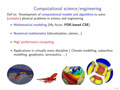
Computational science/engineeringDef’on: Development of computational models and algorithms to solve(complex) physical problems in science and engineering
• Mathematical modelling (My focus: PDE-based CSE)
• Numerical mathematics (discretization, solvers...)
• High performance computing
• Applications in virtually every discipline ( Climate modelling, subsurfacemodelling, geophysics, aeronautics, ...)
1 / 32
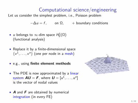
Computational science/engineeringLet us consider the simplest problem, i.e., Poisson problem
−∆u = f , on Ω, + boundary conditions
• u belongs to ∞-dim space H10 (Ω)
(functional analysis)
• Replace it by a finite-dimensional spacev1, . . . , vn (one per node in a mesh)
• e.g., using finite element methods
• The PDE is now approximated by a linearsystem AU = F , where U = [u1, . . . , un]is the vector of nodal values
• A and F are obtained by numericalintegration (in every FE)
2 / 32
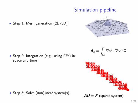
Simulation pipeline
• Step 1: Mesh generation (2D/3D)
• Step 2: Integration (e.g., using FEs) inspace and time
• Step 3: Solve (non)linear system(s)
Aij =
∫Ωi
∇v i · ∇v jdΩ
AU = F (sparse system)3 / 32
Outline
1 Computational Science and Engineering
2 Supercomputing in CSE
3 Multilevel solvers (LSSC-CIMNE)
4 Space-time solvers (LSSC-CIMNE)
5 Conclusions and future work
3 / 32
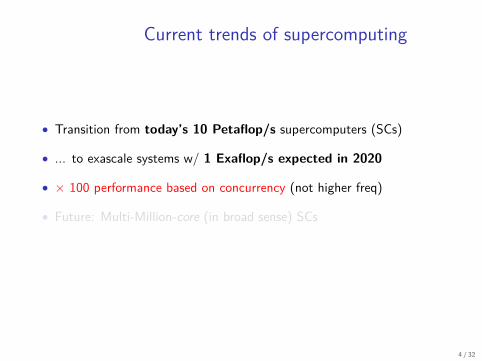
Current trends of supercomputing
• Transition from today’s 10 Petaflop/s supercomputers (SCs)
• ... to exascale systems w/ 1 Exaflop/s expected in 2020
• × 100 performance based on concurrency (not higher freq)
• Future: Multi-Million-core (in broad sense) SCs
4 / 32
Current trends of supercomputing
• Transition from today’s 10 Petaflop/s supercomputers (SCs)
• ... to exascale systems w/ 1 Exaflop/s expected in 2020
• × 100 performance based on concurrency (not higher freq)
• Future: Multi-Million-core (in broad sense) SCs
4 / 32
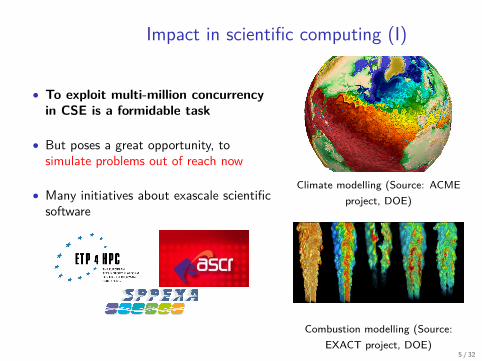
Impact in scientific computing (I)
• To exploit multi-million concurrencyin CSE is a formidable task
• But poses a great opportunity, tosimulate problems out of reach now
• Many initiatives about exascale scientificsoftware
Climate modelling (Source: ACMEproject, DOE)
Combustion modelling (Source:EXACT project, DOE)
5 / 32
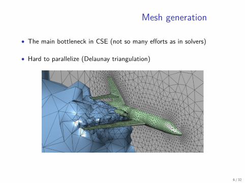
Mesh generation
• The main bottleneck in CSE (not so many efforts as in solvers)
• Hard to parallelize (Delaunay triangulation)
6 / 32
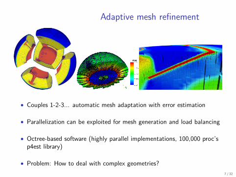
Adaptive mesh refinement
• Couples 1-2-3... automatic mesh adaptation with error estimation
• Parallelization can be exploited for mesh generation and load balancing
• Octree-based software (highly parallel implementations, 100,000 proc’sp4est library)
• Problem: How to deal with complex geometries?7 / 32
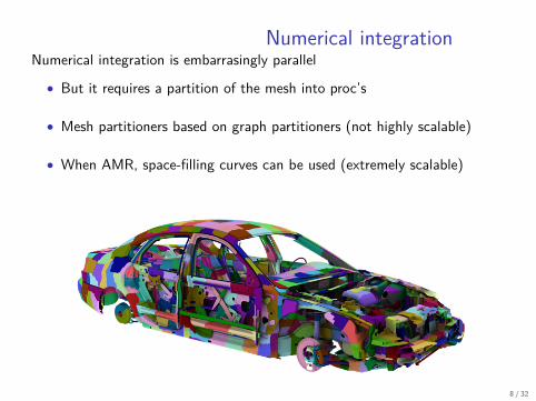
Numerical integrationNumerical integration is embarrasingly parallel
• But it requires a partition of the mesh into proc’s
• Mesh partitioners based on graph partitioners (not highly scalable)
• When AMR, space-filling curves can be used (extremely scalable)
8 / 32
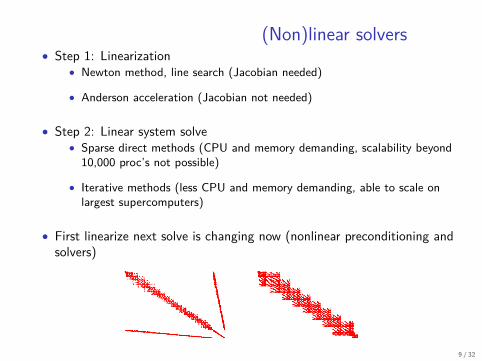
(Non)linear solvers• Step 1: Linearization
• Newton method, line search (Jacobian needed)
• Anderson acceleration (Jacobian not needed)
• Step 2: Linear system solve• Sparse direct methods (CPU and memory demanding, scalability beyond
10,000 proc’s not possible)
• Iterative methods (less CPU and memory demanding, able to scale onlargest supercomputers)
• First linearize next solve is changing now (nonlinear preconditioning andsolvers)
9 / 32
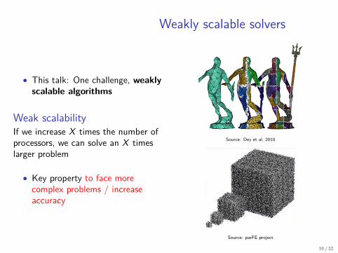
Weakly scalable solvers
• This talk: One challenge, weaklyscalable algorithms
Weak scalabilityIf we increase X times the number ofprocessors, we can solve an X timeslarger problem
• Key property to face morecomplex problems / increaseaccuracy
Source: Dey et al, 2010
Source: parFE project
10 / 32
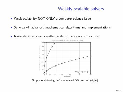
Weakly scalable solvers
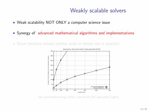
• Weak scalability NOT ONLY a computer science issue
• Synergy of advanced mathematical algorithms and implementations
• Naive iterative solvers neither scale in theory nor in practice
0
50
100
150
200
250
300
350
400
12 48 108 192 300 432 588 768
Num
ber
of P
CG
iter
atio
ns fo
r th
e in
terf
ace
prob
lem
#subdomains
stopc=res+res. rtol=1.0e-06. atol=0.0. Weak scaling with H/h=256
CG no preconditioningNN preconditioner
No preconditioning (left); one-level DD precond (right)
11 / 32
Weakly scalable solvers
• Weak scalability NOT ONLY a computer science issue
• Synergy of advanced mathematical algorithms and implementations
• Naive iterative solvers neither scale in theory nor in practice
0
50
100
150
200
250
300
350
400
12 48 108 192 300 432 588 768
Num
ber
of P
CG
iter
atio
ns fo
r th
e in
terf
ace
prob
lem
#subdomains
stopc=res+res. rtol=1.0e-06. atol=0.0. Weak scaling with H/h=256
CG no preconditioningNN preconditioner
No preconditioning (left); one-level DD precond (right)
11 / 32
Outline
1 Computational Science and Engineering
2 Supercomputing in CSE
3 Multilevel solvers (LSSC-CIMNE)
4 Space-time solvers (LSSC-CIMNE)
5 Conclusions and future work
11 / 32
Scalable linear solvers (AMG)
• Most scalable solvers for CSE are parallel AMG (Trilinos [Lin, Shadid,Tuminaro, ...], Hypre [Falgout, Yang,...],...)
• Hard to scale up to largest SCs today (one million cores, < 10 PFs)
• Largest problems 1011 for unstructured meshes (we are there) and 1013for structured meshes
• Problems: large communication/computation ratios at coarser levels,densification coarser problems,...
12 / 32
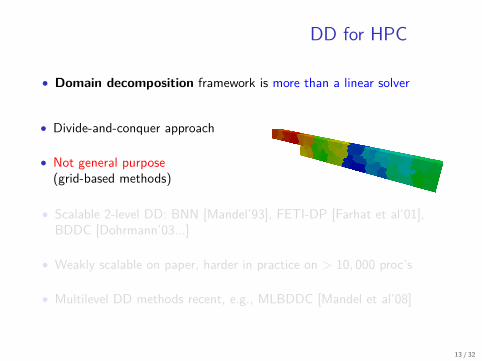
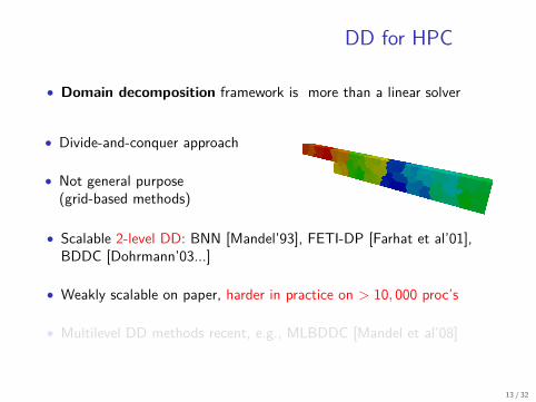
DD for HPC
• Domain decomposition framework is more than a linear solver
• Divide-and-conquer approach
• Not general purpose(grid-based methods)
• Scalable 2-level DD: BNN [Mandel’93], FETI-DP [Farhat et al’01],BDDC [Dohrmann’03...]
• Weakly scalable on paper, harder in practice on > 10, 000 proc’s
• Multilevel DD methods recent, e.g., MLBDDC [Mandel et al’08]
13 / 32
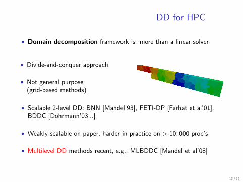
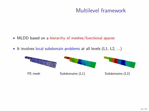
Multilevel framework
• MLDD based on a hierarchy of meshes/functional spaces
• It involves local subdomain problems at all levels (L1, L2, ...)
FE mesh Subdomains (L1) Subdomains (L2)
14 / 32
Outline
• Motivation: Develop a multilevel framework for scalable linear algebra(MLBDDC)
15 / 32
Outline
• Motivation: Develop a multilevel framework for scalable linear algebra(MLBDDC)
All implementations in FEMPAR (in-house code) to be dis-tributed as open-source SW soon*
* Funded by Staring Grant 258443 COMFUS and Proof of Concept Grant 640957 -FEXFEM: On a free open source extreme scale finite element software
15 / 32
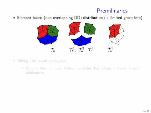
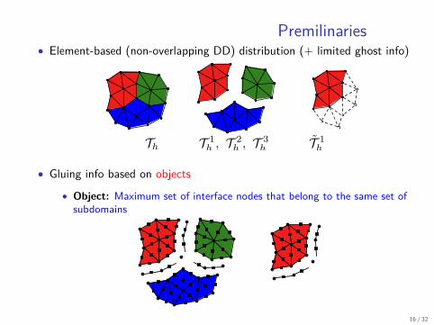
Premilinaries• Element-based (non-overlapping DD) distribution (+ limited ghost info)
Th T 1h , T 2
h , T 3h T 1
h
• Gluing info based on objects
• Object: Maximum set of interface nodes that belong to the same set ofsubdomains
16 / 32
Premilinaries• Element-based (non-overlapping DD) distribution (+ limited ghost info)
Th T 1h , T 2
h , T 3h T 1
h
• Gluing info based on objects
• Object: Maximum set of interface nodes that belong to the same set ofsubdomains
16 / 32
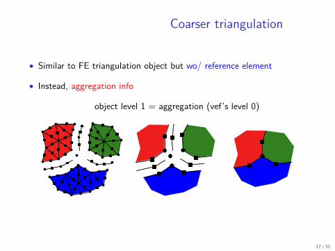
Coarser triangulation
• Similar to FE triangulation object but wo/ reference element
• Instead, aggregation info
object level 1 = aggregation (vef’s level 0)
17 / 32
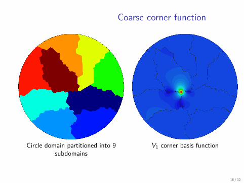
Coarse corner function
Circle domain partitioned into 9subdomains
V1 corner basis function
18 / 32
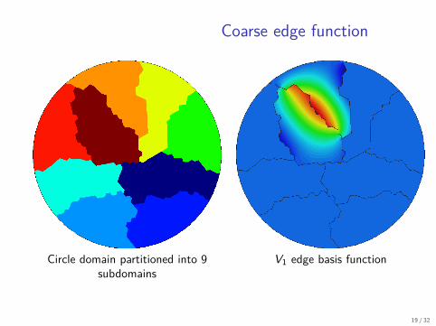
Coarse edge function
Circle domain partitioned into 9subdomains
V1 edge basis function
19 / 32
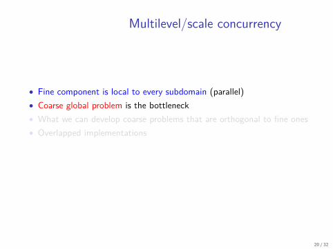
Multilevel/scale concurrency
• Fine component is local to every subdomain (parallel)• Coarse global problem is the bottleneck• What we can develop coarse problems that are orthogonal to fine ones• Overlapped implementations
Multilevel concurrency is BASIC for extreme scalabilityimplementations
20 / 32
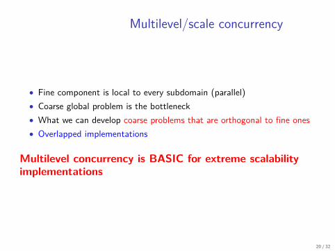
Multilevel concurrency
P0
=
P1 P2
t
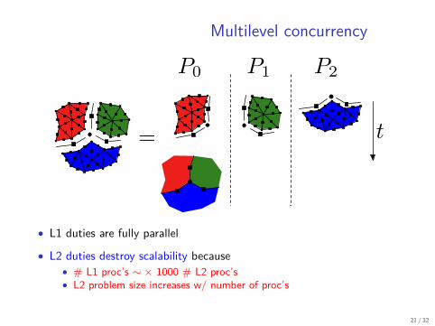
• L1 duties are fully parallel
• L2 duties destroy scalability because• # L1 proc’s ∼ × 1000 # L2 proc’s• L2 problem size increases w/ number of proc’s
21 / 32
Multilevel concurrency
P0
=
P1 P2
t
P3
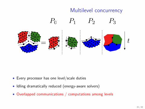
• Every processor has one level/scale duties
• Idling dramatically reduced (energy-aware solvers)
• Overlapped communications / computations among levels
21 / 32
Multilevel concurrency
P0
=
P1 P2
t
P3
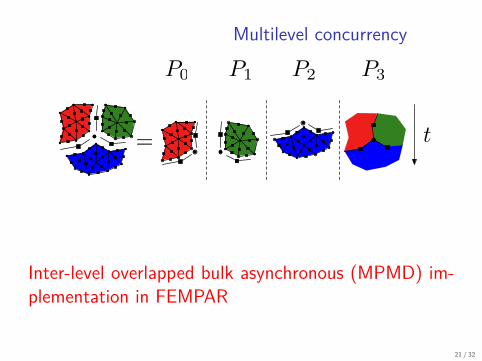
Inter-level overlapped bulk asynchronous (MPMD) im-plementation in FEMPAR
21 / 32
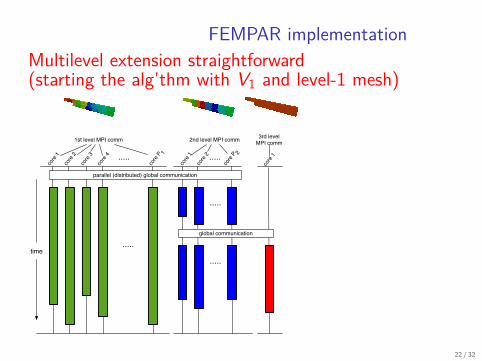
FEMPAR implementationMultilevel extension straightforward(starting the alg’thm with V1 and level-1 mesh)
.....
core
1
core
2
core
3
core
4
core
P 1
1st level MPI comm
.....
.....
core
1
core
2
core
P 2
2nd level MPI comm
.....
3rd level MPI comm
core
1
parallel (distributed) global communication
global communication
.....
time
22 / 32
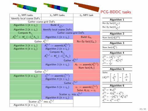
PCG-BDDC tasksL1 MPI tasks L2 MPI tasks L3 MPI task
Identify local coarse DoFsGather coarse-grid DoFs
Algorithm 1 (k ≡ iL1) Build GA
(jL2 )
CAlgorithm 2 (k ≡ iL1) Identify local coarse DoFs
Compute ΦiL1 Gather coarse-grid DoFsA(iL1 )
C ← ΦtiL1
(−CTiL1
ΛiL1 ) Algorithm 1 (k ≡ iL2) Build GAC
Gather A(iL1 )
C Re+Sy fact(GAC)Algorithm 3 (k ≡ iL1) A(jL2 )
C := assemb(A(iL1 )
C )Algorithm 4 (k ≡ iL1) Algorithm 2 (k ≡ iL2)
Compute ΦiL2A(iL2 )
C ← ΦtiL2
(−CTiL2
ΛiL2 )
Gather A(iL2 )
C
Algorithm 3 (k ≡ iL2) AC := assemb(A(iL2 )
C )Num fact(AC)
Gather r (iL1 )
C
Algorithm 5 (k ≡ iL1) r (jL2 )
C := assemb(r (iL1 )
C )Algorithm 4 (k ≡ iL2)
Gather r (iL2 )1
Algorithm 5 (k ≡ iL2) rC := assemb(r (iL2 )
C )Solve ACzC = rC
Scatter zC into z (iL2 )
CAlgorithm 6 (k ≡ iL2)
Scatter z (jL2 )
C into z (iL1 )
CAlgorithm 6 (k ≡ iL1)
Algorithm 1Re+Sy fact(G
A(k)
F)
Re+Sy fact(GA(k)
II)
Algorithm 2Num fact((Ab
0 )(k))
Algorithm 3Num fact(A(k)
II )
Algorithm 4δ
(k)I ← (A(k)
II )−1r (k)I
r (k)Γ ← r (k)
Γ − A(k)ΓI δ
(k)I
r (k) ← Itk r
Algorithm 5Solve
(Ab0 )(k)
[t
s(k)Fλ
]=
[0
r (k)
0
]
Algorithm 6s(k)
C ← Φiz (k)C
z (k) ← Ii(s(k)F + s(k)
C )
z (k)I ← −(A(k)
II )−1A(k)IΓ z (k)
Γ
z (k)I ← z (k)
I + δ(k)I
23 / 32
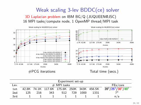
Weak scaling 3-lev BDDC(ce) solver3D Laplacian problem on IBM BG/Q (JUQUEEN@JSC)
16 MPI tasks/compute node, 1 OpenMP thread/MPI task
0
10
20
30
40
50
2.7K 42.8K 117.6K 175.6K 250K 343K 458K
#cores
Weak scaling for MLBDDC(ce) solver
3-lev H1/h1=20 H2/h2=74-lev H1/h1=20 H2/h2=3 H3/h3=3
3-lev H1/h1=25 H2/h2=74-lev H1/h1=25 H2/h2=3 H3/h3=3
3-lev H1/h1=30 H2/h2=73-lev H1/h1=40 H2/h2=7
0
5
10
15
20
2.7K 42.8K 117.6K 175.6K 250K 343K 458K
#cores
30 40 50 60 70 80
2.7K 42.8K 117.6K 175.6K 250K 343K 458K
#cores
Weak scaling for MLBDDC(ce) solver
3-lev H1/h1=40 H2/h2=7
#PCG iterations Total time (secs.)
Experiment set-upLev. # MPI tasks FEs/core1st 42.8K 74.1K 117.6K 175.6K 250K 343K 456.5K 203/253/303/4032nd 125 216 343 512 729 1000 1331 733rd 1 1 1 1 1 1 1 n/a
24 / 32
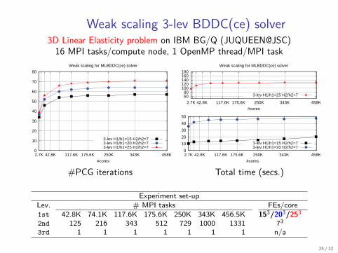
Weak scaling 3-lev BDDC(ce) solver3D Linear Elasticity problem on IBM BG/Q (JUQUEEN@JSC)16 MPI tasks/compute node, 1 OpenMP thread/MPI task
0
10
20
30
40
50
60
70
80
2.7K 42.8K 117.6K 175.6K 250K 343K 458K
#cores
Weak scaling for MLBDDC(ce) solver
3-lev H1/h1=15 H2/h2=73-lev H1/h1=20 H2/h2=73-lev H1/h1=25 H2/h2=7
0
10
20
30
40
50
2.7K 42.8K 117.6K 175.6K 250K 343K 458K
#cores
3-lev H1/h1=15 H2/h2=73-lev H1/h1=20 H2/h2=7
60 80
100 120 140 160 180
2.7K 42.8K 117.6K 175.6K 250K 343K 458K
#cores
Weak scaling for MLBDDC(ce) solver
3-lev H1/h1=25 H2/h2=7
#PCG iterations Total time (secs.)
Experiment set-upLev. # MPI tasks FEs/core1st 42.8K 74.1K 117.6K 175.6K 250K 343K 456.5K 153/203/2532nd 125 216 343 512 729 1000 1331 733rd 1 1 1 1 1 1 1 n/a
25 / 32
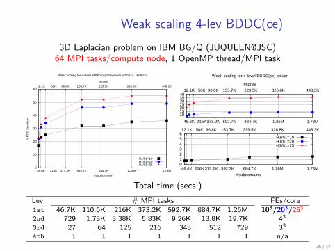
Weak scaling 4-lev BDDC(ce)3D Laplacian problem on IBM BG/Q (JUQUEEN@JSC)
64 MPI tasks/compute node, 1 OpenMP thread/MPI task
0
10
20
30
40
50
60
46.6K 216K 373.2K 592.7K 884.7K 1.26M 1.73M
12.1K 56K 96.8K 153.7K 229.5K 326.8K 448.3K
# P
CG
iter
atio
ns
#subdomains
Weak scaling for 4-level BDDC(ce) solver with H2/h2=4, H3/h3=3
#cores
H1/h1=10H1/h1=20H1/h1=25 0
1 2 3 4 5 6
46.6K 216K373.2K 592.7K 884.7K 1.26M 1.73M
12.1K 56K 96.8K 153.7K 229.5K 326.8K 448.3K
#subdomains
H1/h1=10H1/h1=20H1/h1=25
10 15 20 25 30 35 40
46.6K 216K373.2K 592.7K 884.7K 1.26M 1.73M
12.1K 56K 96.8K 153.7K 229.5K 326.8K 448.3K
Weak scaling for 4-level BDDC(ce) solver
#cores
Total time (secs.)Lev. # MPI tasks FEs/core1st 46.7K 110.6K 216K 373.2K 592.7K 884.7K 1.26M 103/203/2532nd 729 1.73K 3.38K 5.83K 9.26K 13.8K 19.7K 433rd 27 64 125 216 343 512 729 334th 1 1 1 1 1 1 1 n/a
26 / 32
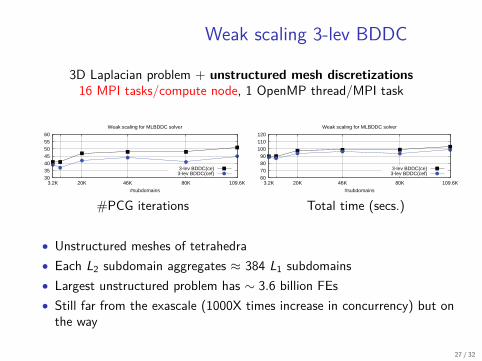
Weak scaling 3-lev BDDC
3D Laplacian problem + unstructured mesh discretizations16 MPI tasks/compute node, 1 OpenMP thread/MPI task
30 35 40 45 50 55 60
3.2K 20K 46K 80K 109.6K
#subdomains
Weak scaling for MLBDDC solver
3-lev BDDC(ce)3-lev BDDC(cef)
60 70 80 90
100 110 120
3.2K 20K 46K 80K 109.6K
#subdomains
Weak scaling for MLBDDC solver
3-lev BDDC(ce)3-lev BDDC(cef)
#PCG iterations Total time (secs.)
• Unstructured meshes of tetrahedra• Each L2 subdomain aggregates ≈ 384 L1 subdomains• Largest unstructured problem has ∼ 3.6 billion FEs• Still far from the exascale (1000X times increase in concurrency) but onthe way
27 / 32
Outline
1 Computational Science and Engineering
2 Supercomputing in CSE
3 Multilevel solvers (LSSC-CIMNE)
4 Space-time solvers (LSSC-CIMNE)
5 Conclusions and future work
27 / 32
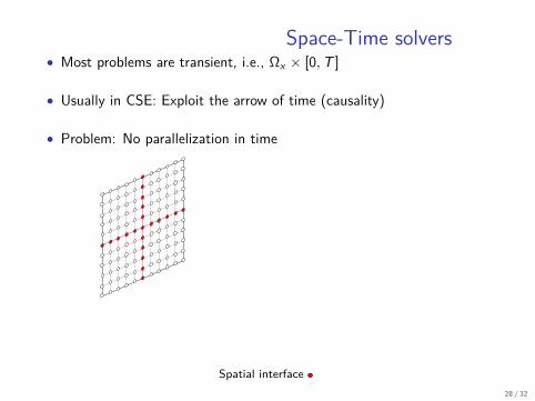
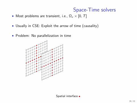
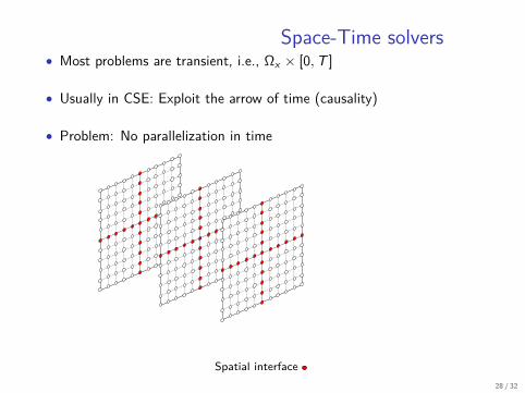
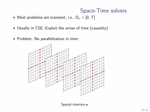
Space-Time solvers• Most problems are transient, i.e., Ωx × [0, T ]
• Usually in CSE: Exploit the arrow of time (causality)
• Problem: No parallelization in time
Spatial interface28 / 32
Space-Time solvers• Most problems are transient, i.e., Ωx × [0, T ]
• Usually in CSE: Exploit the arrow of time (causality)
• Problem: No parallelization in time
Spatial interface28 / 32
Space-Time solvers• Most problems are transient, i.e., Ωx × [0, T ]
• Usually in CSE: Exploit the arrow of time (causality)
• Problem: No parallelization in time
Spatial interface28 / 32
Space-Time solvers• Most problems are transient, i.e., Ωx × [0, T ]
• Usually in CSE: Exploit the arrow of time (causality)
• Problem: No parallelization in time
Spatial interface28 / 32
Why space-time parallelism?• Increasing number of available processors (exascale)
• Spatial parallelization saturates at some point
• Many problems require heavy time-stepping (additive manufacturing,turbulent flows)
29 / 32
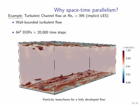
Why space-time parallelism?Example: Turbulent Channel flow at Reτ = 395 (implicit LES)
• Wall-bounded turbulent flow
• 643 DOFs × 20,000 time steps
Vorticity isosurfaces for a fully developed flow29 / 32
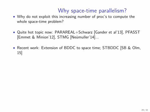
Why space-time parallelism?• Why do not exploit this increasing number of proc’s to compute thewhole space-time problem?
• Quite hot topic now: PARAREAL+Schwarz [Gander et al’13], PFASST[Emmet & Minion’12], STMG [Neümuller’14]...
• Recent work: Extension of BDDC to space time; STBDDC [SB & Olm,15]
29 / 32
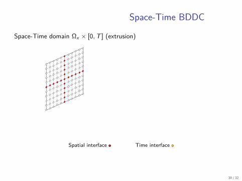
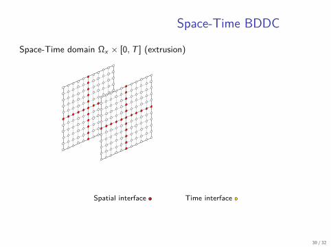
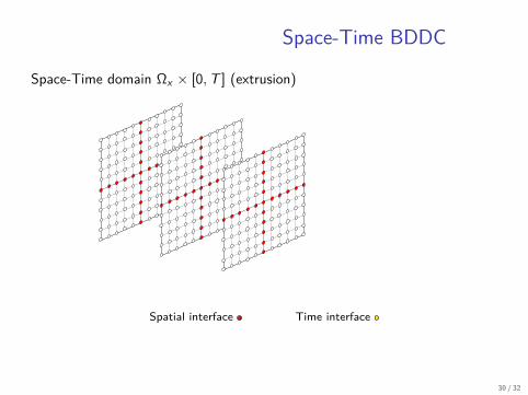
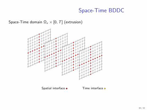
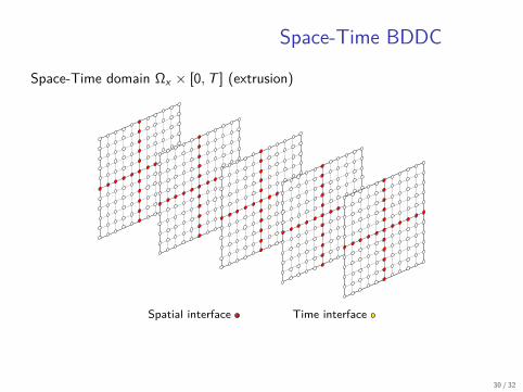
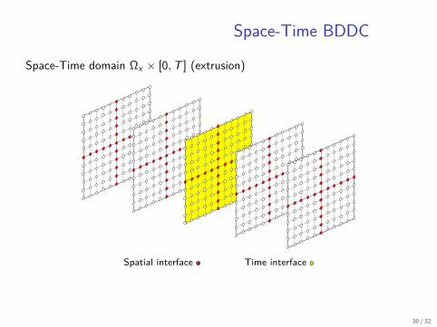
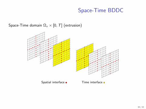
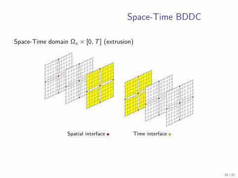
Space-Time BDDC
Space-Time domain Ωx × [0, T ] (extrusion)
Spatial interface Time interface
30 / 32
Space-Time BDDC
Space-Time domain Ωx × [0, T ] (extrusion)
Spatial interface Time interface
30 / 32
Space-Time BDDC
Space-Time domain Ωx × [0, T ] (extrusion)
Spatial interface Time interface
30 / 32
Space-Time BDDC
Space-Time domain Ωx × [0, T ] (extrusion)
Spatial interface Time interface
30 / 32
Space-Time BDDC
Space-Time domain Ωx × [0, T ] (extrusion)
Spatial interface Time interface
30 / 32
Space-Time BDDC
Space-Time domain Ωx × [0, T ] (extrusion)
Spatial interface Time interface
30 / 32
Space-Time BDDC
Space-Time domain Ωx × [0, T ] (extrusion)
Spatial interface Time interface
30 / 32
Space-Time BDDC
Space-Time domain Ωx × [0, T ] (extrusion)
Spatial interface Time interface
30 / 32
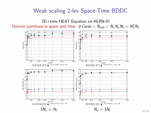
Weak scaling 2-lev Space-Time BDDC2D+time HEAT Equation on HLRN-III
Domain partitions in space and time: #Cores = Nsub = NxNyNt = N2xNt
0
2
4
6
8
10
12
14
16
18
375 1029 1536 2187 3000 3993
#Ite
ratio
ns
#CoresH/h=30 T/δt=30, CFL=3H/h=40 T/δt=40, CFL=4
H/h=40 T/δt=20, CFL=8
0
2
4
6
8
10
12
14
16
243 576 1125 1944 3087 4608
#Ite
ratio
ns
#CoresH/h=30 T/δt=30, CFL=3H/h=40 T/δt=40, CFL=4
H/h=40 T/δt=20, CFL=8
0
5
10
15
20
25
30
35
40
375 1029 1536 2187 3000 3993
Wal
l clo
ck ti
me
(s)
#CoresH/h=30 T/δt=30, CFL=3H/h=40 T/δt=40, CFL=4
H/h=40 T/δt=20, CFL=8
0
5
10
15
20
25
30
35
40
243 576 1125 1944 3087 4608
Wal
l clo
ck ti
me
(s)
#CoresH/h=30 T/δt=30, CFL=3H/h=40 T/δt=40, CFL=4
H/h=40 T/δt=20, CFL=8
3Nx = Nt Nx = 3Nt 31 / 32
Farewell
Thank you!SB, A. F. Martín and J. Principe. Multilevel Balancing Domain Decomposition atExtreme Scales. Submitted, 2015.
SB, A. F. Martín and J. Principe. A highly scalable parallel implementation ofbalancing domain decomposition by constraints. SIAM Journal on ScientificComputing. Vol. 36(2), pp. C190-C218, 2014.
SB, A. F. Martín and J. Principe. On the scalability of inexact balancing domaindecomposition by constraints with overlapped coarse/fine corrections. ParallelComputing, in press, 2015.
SB, M. Olm. Space-time balacing domain decomposition. Submitted, 2015.
Work funded by the European Research Council under:
• Starting Grant 258443 - COMFUS: Computational Methodsfor Fusion Technology
• Proof of Concept Grant 640957 - FEXFEM: On a free opensource extreme scale finite element software
2007 - 2012
European Research CouncilYears of excellent IDEAS
31 / 32
Outline
1 Computational Science and Engineering
2 Supercomputing in CSE
3 Multilevel solvers (LSSC-CIMNE)
4 Space-time solvers (LSSC-CIMNE)
5 Conclusions and future work
31 / 32
Conclusions and future workBrief introduction to CSE
• Three setps in CSE: Mesh / Integration / Nonlinear solver• Challenges at the exascale
Our research at LSSC-CIMNE• Multilevel domain decomposition solvers• Space-time solvers• Highly scalable FEMPAR library (to be released in October)
Other exciting topics:• Embedded boundary method (eliminates unstructured mesh for complexgeometries)
• Nonlinear space-time preconditioning• Highly heterogeneous (subsurface modelling) and multiphysicspreconditioners (MHD, fluid-structure, etc)
32 / 32