summer review for algebra ii
TRANSCRIPT

Summer Review
For Students Entering Algebra 2

2
Board of Education of Howard County
Frank Aquino Chairman
Ellen Flynn Giles Larry Cohen Vice Chairman Allen Dyer Sandra H. French Patricia S. Gordon Janet Siddiqui
Sydney L. Cousin Superintendent of Schools
Copyright 2010
The Howard County Public School System Ellicott City, Maryland 21042
3
INTRODUCTION
Teachers and administrators in the Howard County Public School System actively encourage parents and community members to engage in children’s learning. This Summer Review For Students Entering Algebra 2 has been developed to provide friends, family, and community members a summer resource to help students reach their full potential. The packet has been designed to provide a review of Algebra 1 skills that are essential for student success in Algebra 2. The Howard County Office of Mathematics recommends that students complete this booklet during the summer and bring it, with work shown, to school on the first day of Algebra 2. Assistance with the packet will be provided at the beginning of the school year. Completion of this packet over the summer before beginning Algebra 2 will be of great value to helping students successfully meet the academic challenges awaiting them in Algebra 2 and beyond. These challenges include
• The Preliminary Scholastic Aptitude Test (PSAT), Scholastic Aptitude Test (SAT) I and II, and American College Test (ACT)
• College placement and advanced placement (AP) tests. Resources included in this packet are the following:
• A listing of the Algebra 1/ Data Analysis objectives students need to have mastered to be successful in Algebra 2,
• A set of problems emphasizing important objectives from the Algebra 1/Data Analysis curriculum that will help students prepare for Algebra 2,
• Answers to those problems. Directions:
• Students are requested to work in pencil and show their work in the packet or on lined paper to accompany the packet. They should check their answers using the key provided and, if possible, correct the work for problems solved incorrectly. Round answers to the nearest tenth.
• A calculator may be used on any of the problems in this packet and a graphing calculator is required for some.
Families are encouraged to use the many resources available at the following websites:
• http://www2.hcpss.org/math/smart and click on Secondary Mathematics Internet Resources – has links to dozens of mathematics related websites containing activities, tutorials, games, puzzles and lists of resources.
• http://www.howa.lib.md.us/ -- offers free access to Live Homework Help, providing
assistance at all levels of mathematics.
• http://www.algebrahelp.com/ -- offers assistance on various algebra topics

4
Algebra 1 Skills Needed to be Successful in Algebra 2
A. Simplifying Polynomial Expressions
Objectives: The student will be able to: • Apply the appropriate arithmetic operations and algebraic properties needed to
simplify an algebraic expression. • Simplify polynomial expressions using addition and subtraction. • Multiply a monomial and polynomial.
B. Solving Equations Objectives: The student will be able to: • Solve multi-step equations. • Solve a literal equation for a specific variable, and use formulas to solve problems.
C. Rules of Exponents
Objectives: The student will be able to: • Simplify expressions using the laws of exponents. • Evaluate powers that have zero or negative exponents.
D. Binomial Multiplication
Objectives: The student will be able to: • Multiply two binomials.
E. Factoring
Objectives: The student will be able to: • Identify the greatest common factor of the terms of a polynomial expression. • Express a polynomial as a product of a monomial and a polynomial. • Find all factors of the quadratic expression ax2 + bx + c by factoring and graphing.
F. Radicals Objectives: The student will be able to: • Simplify radical expressions.
G. Graphing Lines
Objectives: The student will be able to: • Identify and calculate the slope of a line. • Graph linear equations using a variety of methods. • Determine the equation of a line.
H. Regression and Use of the Graphing Calculator
Objectives: The student will be able to: • Draw a scatter plot, find the line of best fit, and use it to make predictions. • Graph and interpret real-world situations using linear models.
5
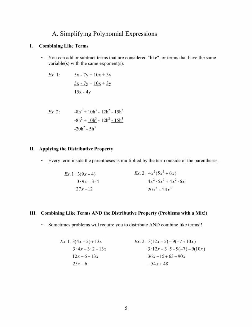
A. Simplifying Polynomial Expressions
I. Combining Like Terms
- You can add or subtract terms that are considered "like", or terms that have the same variable(s) with the same exponent(s).
Ex. 1: 5x - 7y + 10x + 3y
5x - 7y + 10x + 3y
15x - 4y
Ex. 2: -8h2 + 10h3 - 12h2 - 15h3
-8h2 + 10h3 - 12h2 - 15h3
-20h2 - 5h3
II. Applying the Distributive Property
- Every term inside the parentheses is multiplied by the term outside of the parentheses.
!
Ex. 1: 3(9x " 4)
3 # 9x " 3 # 4
27x "12
!
Ex. 2 : 4x2(5x
3+ 6x)
4x2" 5x
3+ 4x
2" 6x
20x5
+ 24x3
III. Combining Like Terms AND the Distributive Property (Problems with a Mix!)
- Sometimes problems will require you to distribute AND combine like terms!!
!
Ex. 1: 3(4x " 2) +13x
3 # 4x " 3 # 2 +13x
12x " 6 +13x
25x " 6
!
Ex. 2 : 3(12x " 5) " 9("7 +10x)
3 #12x " 3 # 5" 9("7) " 9(10x)
36x "15+ 63" 90x
" 54x + 48
6
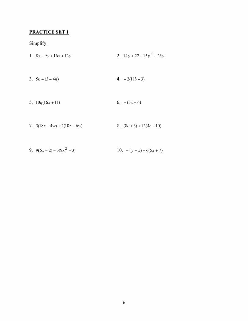
PRACTICE SET 1 Simplify. 1. yxyx 121698 ++! 2. yyy 23152214
2+!+
3. )43(5 nn !! 4. )311(2 !! b 5. )1116(10 +xq 6. )65( !! x 7. )610(2)418(3 wzwz !+! 8. )104(12)38( !++ cc 9. )39(3)26(9 2
!!! xx 10. )75(6)( ++!! xxy
7
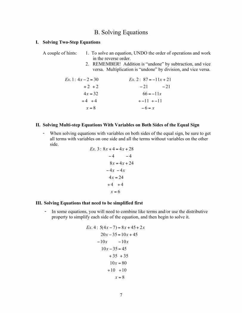
B. Solving Equations I. Solving Two-Step Equations
A couple of hints: 1. To solve an equation, UNDO the order of operations and work in the reverse order.
2. REMEMBER! Addition is “undone” by subtraction, and vice versa. Multiplication is “undone” by division, and vice versa.
!
Ex. 1: 4x " 2 = 30
+ 2 + 2
4x = 32
÷ 4 ÷ 4
x = 8
!
Ex. 2 : 87 = "11x + 21
" 21 " 21
66 = "11x
÷"11 ÷"11
" 6 = x
II. Solving Multi-step Equations With Variables on Both Sides of the Equal Sign
- When solving equations with variables on both sides of the equal sign, be sure to get all terms with variables on one side and all the terms without variables on the other side.
!
Ex. 3 : 8x + 4 = 4x + 28
" 4 " 4
8x = 4x + 24
" 4x " 4x
4x = 24
÷ 4 ÷ 4
x = 6
III. Solving Equations that need to be simplified first
- In some equations, you will need to combine like terms and/or use the distributive property to simplify each side of the equation, and then begin to solve it.
!
Ex. 4 : 5(4x " 7) = 8x + 45+ 2x
20x " 35 =10x + 45
"10x "10x
10x " 35 = 45
+ 35 + 35
10x = 80
÷10 ÷10
x = 8

8
PRACTICE SET 2 Solve each equation. You must show all work.
1. 3325 =!x 2. 364140 += x 3. 196)43(8 =!x 4. 601572045 =+! xx 5. )912(4132 != x 6. 687154198 !+= x 7. xx 6)83(5131 +!!=! 8. xx 318107 +=!! 9. )823(215812 !!=!+ xx 10. 612)612( +=!! xx
IV. Solving Literal Equations
- A literal equation is an equation that contains more than one variable. - You can solve a literal equation for one of the variables by getting that variable by itself
(isolating the specified variable).
!
Ex. 1: 3xy =18, Solve for x.
3xy
3y=
18
3y
x =6
y
!
Ex. 2 : 5a "10b = 20, Solve for a.
+10b =+10b
5a = 20 +10b
5a
5=
20
5+
10b
5
a = 4 + 2b

9
PRACTICE SET 3 Solve each equation for the specified variable. 1. Y + V = W, for V 2. 9wr = 81, for w 3. 2d – 3f = 9, for f 4. dx + t = 10, for x 5. P = (g – 9)180, for g 6. 4x + y – 5h = 10y + u, for x

10
C. Rules of Exponents Multiplication: Recall )()()( nmnm
xxx+
= Ex:
!
(3x4y
2 )(4xy5 )=(3 " 4)(x
4" x
1)( y2" y
5 )=12x5y
7
Division: Recall )( nm
n
m
xx
x != Ex: jm
j
j
m
m
jm
jm 2
1
2
3
5
3
25
143
42
3
42!=""
#
$%%&
'""#
$%%&
'"#
$%&
'
!=
!
Powers: Recall )()( nmnm
xx!
= Ex: 12393431333343 8)()()()2()2( cbacbabca !=!=! Power of Zero: Recall 0,1
0!= xx Ex: 4440 5))(1)(5(5 yyyx ==
PRACTICE SET 4 Simplify each expression.
1. ))()(( 25ccc 2.
3
15
m
m 3. 54 )(k
4. 0d 5. ))(( 5724
qpqp 6. zy
zy3
103
5
45
7. 37 )( t! 8. 03
3 gf 9. )15)(4( 3235hkkh
10. cab
ba
2
64
36
12 11. 42 )3( nm 12. 02 )12( yx
13. )3)(2)(5( 22
bcabba !! 14. 02 )2(4 yxx 15. 324 )2)(3( yyx

11
First
!
x " x ------> x2 Outer x·10 -----> 10x Inner 6·x ------> 6x Last 6·10 -----> 60
x2 + 10x + 6x + 60
x2 + 16x + 60 (After combining like terms)
D. Binomial Multiplication
I. Reviewing the Distributive Property
The distributive property is used when you want to multiply a single term by an expression.
xx
xx
xxEx
7240
)9(858
)95(8:1
2
2
2
!
!"+"
!
II. Multiplying Binomials – the FOIL method
When multiplying two binomials (an expression with two terms), we use the “FOIL” method. The “FOIL” method uses the distributive property twice!
FOIL is the order in which you will multiply your terms. First
Outer
Inner
Last
Ex. 1: (x + 6)(x + 10)
LAST INNER
OUTER FIRST
(x + 6)(x + 10)

12
Recall: 42 = 4 · 4
x2 = x · x
Ex. (x + 5)2
(x + 5)2 = (x + 5)(x+5) Now you can use the “FOIL” method to get a simplified expression.
PRACTICE SET 5 Multiply. Write your answer in simplest form. 1. (x + 10)(x – 9) 2. (x + 7)(x – 12) 3. (x – 10)(x – 2) 4. (x – 8)(x + 81) 5. (2x – 1)(4x + 3) 6. (-2x + 10)(-9x + 5) 7. (-3x – 4)(2x + 4) 8. (x + 10)2 9. (-x + 5)2 10. (2x – 3)2

13
E. Factoring
I. Using the Greatest Common Factor (GCF) to Factor.
• Always determine whether there is a greatest common factor (GCF) first.
Ex. 1 23490333 xxx +!
In this example the GCF is 2
3x . So when we factor, we have )3011(3 22
+! xxx . Now we need to look at the polynomial remaining in the parentheses. Can
this trinomial be factored into two binomials? In order to determine this make a list of all of the factors of 30.
Since -5 + -6 = -11 and (-5)(-6) = 30 we should choose -5 and -6 in order to factor the expression.
The expression factors into )6)(5(3 2
!! xxx
Note: Not all expressions will have a GCF. If a trinomial expression does not have a GCF, proceed by trying to factor the trinomial into two binomials.
II. Applying the difference of squares: ( )( )bababa +!=!22
!
Ex. 2 4x3"100x
4x x2" 25( )
4x x " 5( ) x + 5( )
30
1 30 2 15 3 10 5 6
Since 2x and 25 are perfect squares separated by a
subtraction sign, you can apply the difference of two squares formula.
30
-1 -30 -2 -15 -3 -10 -5 -6

14
PRACTICE SET 6
Factor each expression.
1. xx 632+ 2. cababba
23228164 +!
3. 252!x 4. 158
2++ nn
5. 2092
+! gg 6. 2832
!+ dd
7. 3072
!! zz 8. 81182
++ mm
9. yy 3643! 10. 135305
2!+ kk

15
This is not simplified completely because 12 is divisible by 4 (another perfect square)
F. Radicals
To simplify a radical, we need to find the greatest perfect square factor of the number under the radical sign (the radicand) and then take the square root of that number.
PRACTICE SET 7 Simplify each radical. 1. 121 2. 90 3. 175 4. 288 5. 486 6. 2 16 7. 6 500
8. 3 147 9. 8 475 10. 1259
!
Ex. 3 : 48
4 12
2 12
2 4 3
2 " 2 " 3
4 3
!
Ex. 1: 72
36 " 2
6 2
!
Ex. 2 : 4 90
4 " 9 " 10
4 " 3 " 10
12 10
!
Ex. 3 : 48
16 3
4 3
OR

16
G. Graphing Lines I. Finding the Slope of the Line that Contains each Pair of Points.
Given two points with coordinates ( )11, yx and ( )22 , yx , the formula for the slope, m, of
the line containing the points is 12
12
xx
yym
!
!= .
Ex. (2, 5) and (4, 1) Ex. (-3, 2) and (2, 3)
22
4
24
51!=
!=
!
!=m
5
1
)3(2
23=
!!
!=m
The slope is -2. The slope is 5
1
PRACTICE SET 8 1. (-1, 4) and (1, -2) 2. (3, 5) and (-3, 1) 3. (1, -3) and (-1, -2) 4. (2, -4) and (6, -4) 5. (2, 1) and (-2, -3) 6. (5, -2) and (5, 7)

17
II. Using the Slope – Intercept Form of the Equation of a Line. The slope-intercept form for the equation of a line with slope m and y-intercept b is bmxy += .
Ex. 13 != xy Ex. 24
3+!= xy
Slope: 3 y-intercept: -1 Slope: 4
3! y-intercept: 2
Place a point on the y-axis at -1. Place a point on the y-axis at 2. Slope is 3 or 3/1, so travel up 3 on Slope is -3/4 so travel down 3 on the the y-axis and over 1 to the right. y-axis and over 4 to the right. Or travel up 3 on the y-axis and over 4 to the left. PRACTICE SET 9
1. 52 += xy 2. 32
1!= xy
Slope: _____ y-intercept: _____ Slope: _____ y-intercept: _____
x
y y
x
y
x x
y

18
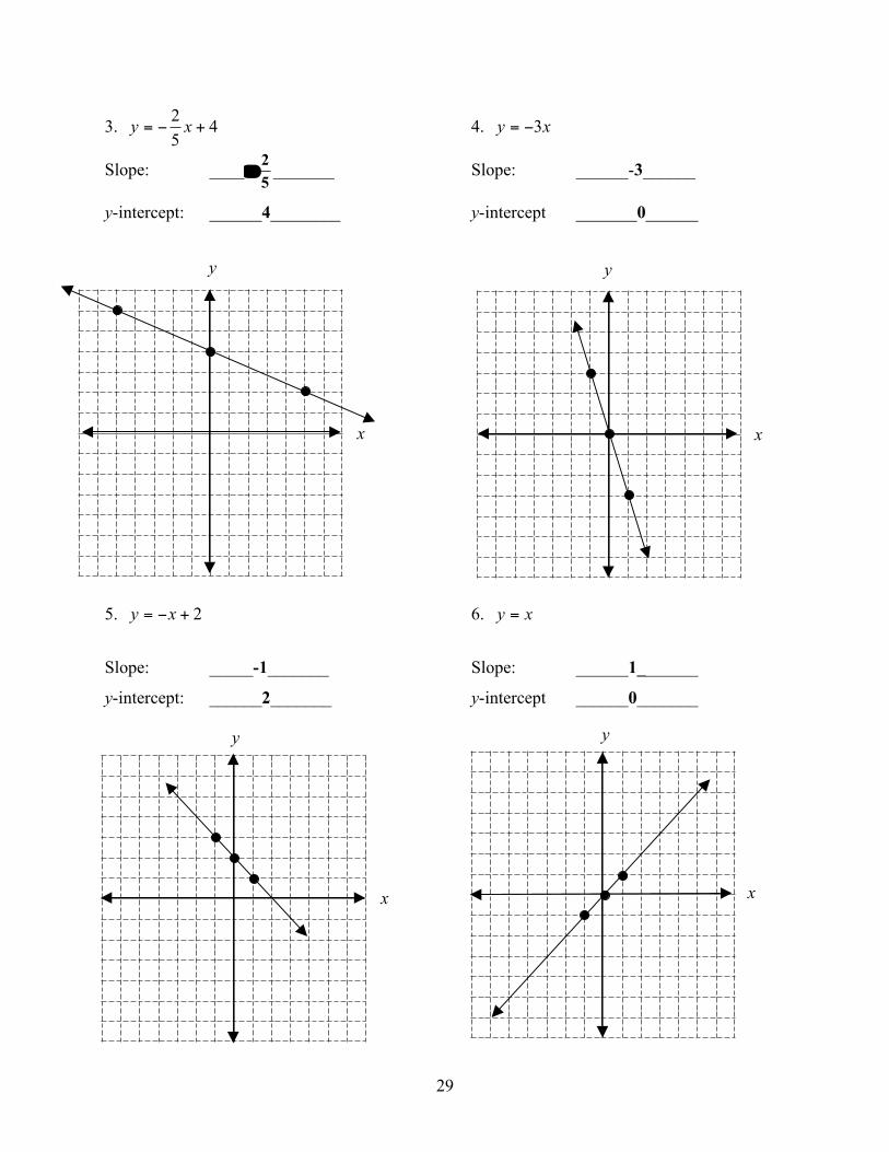
3. 45
2+!= xy 4. xy 3!=
Slope: ______________ Slope: ______________
y-intercept: ______________ y-intercept ______________ 5. 2+!= xy 6. xy =
Slope: ______________ Slope: ______________
y-intercept: ______________ y-intercept ______________
y
x x
y
x
y
x
y

19
III. Using Standard Form to Graph a Line. An equation in standard form can be graphed using several different methods. Two methods are explained below.
a. Re-write the equation in bmxy += form, identify the y-intercept and slope, then graph as in Part II above.
b. Solve for the x- and y- intercepts. To find the x-intercept, let y = 0 and solve for x. To
find the y-intercept, let x = 0 and solve for y. Then plot these points on the appropriate axes and connect them with a line.
Ex. 1032 =! yx a. Solve for y. OR b. Find the intercepts:
1023 +!=! xy let y = 0 : let x = 0:
3
102
!
+!=
xy 10)0(32 =!x 103)0(2 =! y
3
10
3
2!= xy 102 =x 103 =! y
5=x 3
10!=y
So x-intercept is (5, 0) So y-intercept is !"
#$%
&'3
10,0
On the x-axis place a point at 5.
On the y-axis place a point at 3
13
3
10!=!
Connect the points with the line.
y
x

20
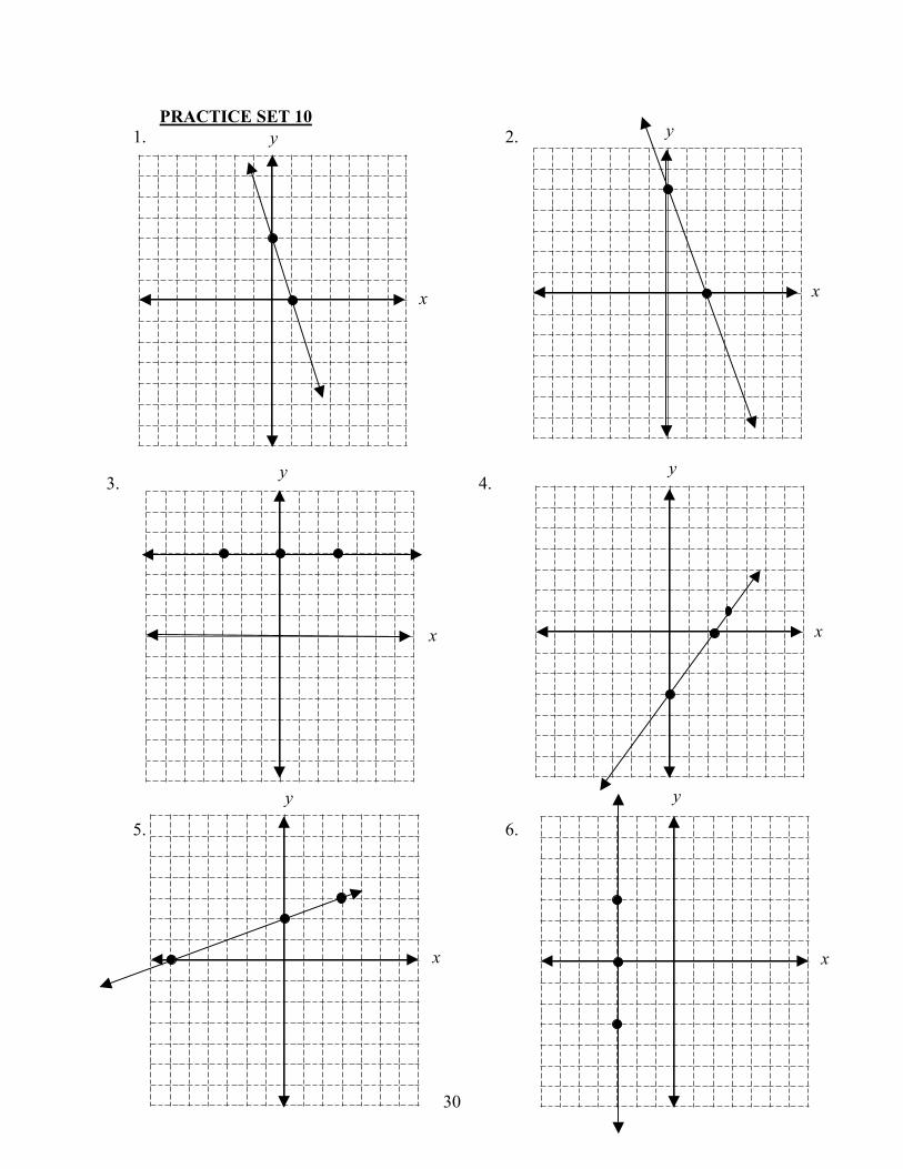
PRACTICE SET 10 1. 33 =+ yx 2. 1025 =+ yx 3. 4=y 4. 934 =! yx
x
y
x
y
x
y
x
y
21
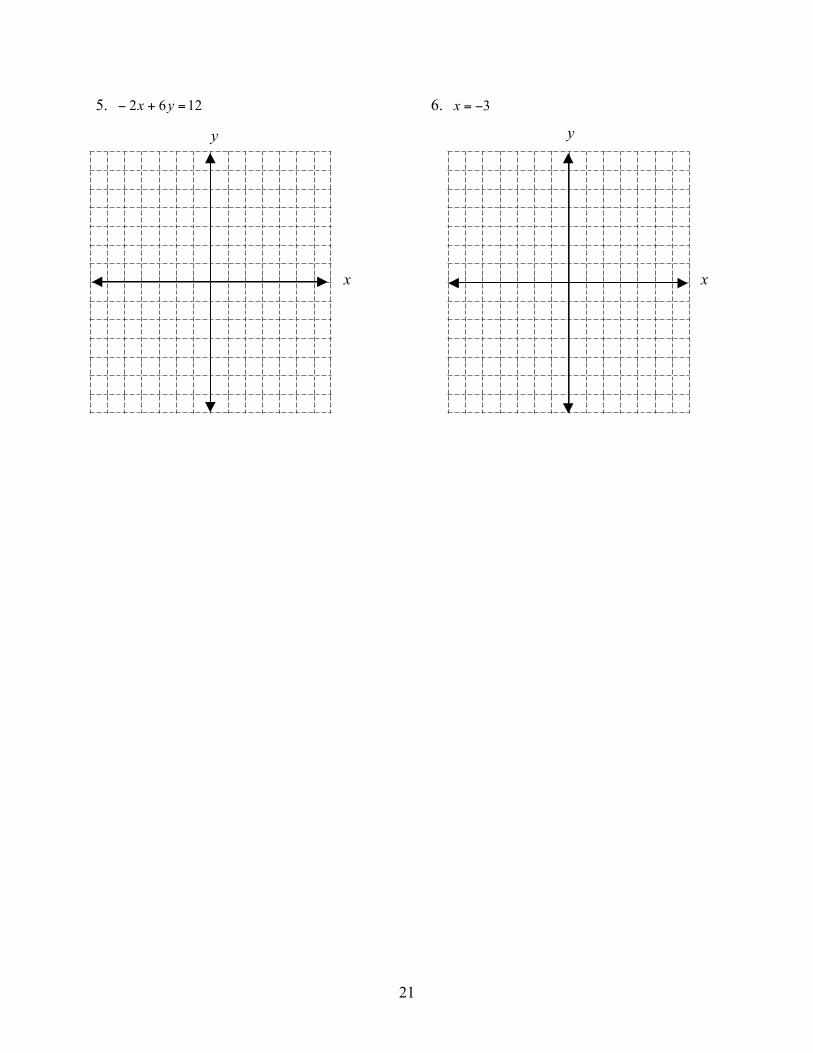
5. 1262 =+! yx 6. 3!=x
y
x
y
x
22
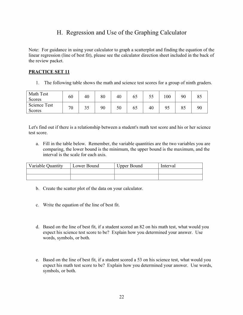
H. Regression and Use of the Graphing Calculator
Note: For guidance in using your calculator to graph a scatterplot and finding the equation of the linear regression (line of best fit), please see the calculator direction sheet included in the back of the review packet. PRACTICE SET 11
1. The following table shows the math and science test scores for a group of ninth graders.
Math Test Scores 60 40 80 40 65 55 100 90 85
Science Test Scores 70 35 90 50 65 40 95 85 90
Let's find out if there is a relationship between a student's math test score and his or her science test score.
a. Fill in the table below. Remember, the variable quantities are the two variables you are comparing, the lower bound is the minimum, the upper bound is the maximum, and the interval is the scale for each axis.
Variable Quantity Lower Bound Upper Bound Interval
b. Create the scatter plot of the data on your calculator. c. Write the equation of the line of best fit.
d. Based on the line of best fit, if a student scored an 82 on his math test, what would you expect his science test score to be? Explain how you determined your answer. Use words, symbols, or both.
e. Based on the line of best fit, if a student scored a 53 on his science test, what would you expect his math test score to be? Explain how you determined your answer. Use words, symbols, or both.
23
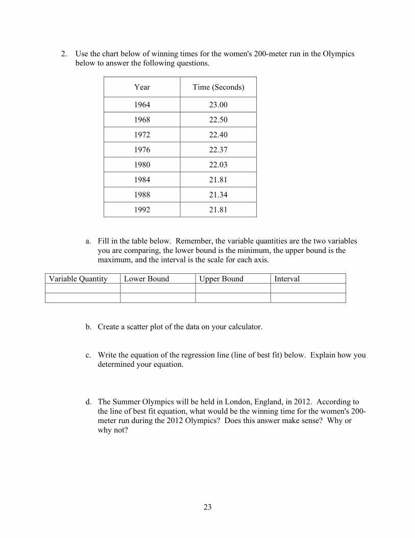
2. Use the chart below of winning times for the women's 200-meter run in the Olympics below to answer the following questions.
Year Time (Seconds)
1964 23.00
1968 22.50
1972 22.40
1976 22.37
1980 22.03
1984 21.81
1988 21.34
1992 21.81
a. Fill in the table below. Remember, the variable quantities are the two variables you are comparing, the lower bound is the minimum, the upper bound is the maximum, and the interval is the scale for each axis.
Variable Quantity Lower Bound Upper Bound Interval
b. Create a scatter plot of the data on your calculator.
c. Write the equation of the regression line (line of best fit) below. Explain how you determined your equation.
d. The Summer Olympics will be held in London, England, in 2012. According to the line of best fit equation, what would be the winning time for the women's 200-meter run during the 2012 Olympics? Does this answer make sense? Why or why not?

24
TI-83 Plus/TI-84 Graphing Calculator Tips How to …
…graph a function Press the Y= key, Enter the function directly using the nTX ,,, ! key to input x. Press the GRAPH key to view the function. Use the WINDOW key to change the dimensions
and scale of the graph. Pressing TRACE lets you move the cursor along the function with the arrow keys to display exact coordinates.
…find the y-value of any x-value Once you have graphed the function, press CALC 2nd TRACE and select 1:value. Enter the x-value. The corresponding y-value is displayed and the cursor
moves to that point on the function.
…find the maximum value of a function Once you have graphed the function, press CALC 2nd TRACE and select 4:maximum. You can set the left and right boundaries of the area to be examined and guess the maximum value either by entering values
directly or by moving the cursor along the function and pressing ENTER. The x-value and y-value of the point with the maximum y-value are then displayed.
…find the zero of a function Once you have graphed the function, press CALC 2nd TRACE and select 2:zero. You can set the left and right boundaries of the root to be examined and guess the value either by entering values
directly or by moving the cursor along the function and pressing ENTER. The x-value displayed is the root.
…find the intersection of two functions Once you have graphed the function, press CALC 2nd TRACE and select 5:intersect. Use the up and down arrows to move among functions and press ENTER to select two. Next,
enter a guess for the point of intersection or move the cursor to an estimated point and press ENTER. The x-value and y-value of the intersection are then displayed.
…enter lists of data Press the STAT key and select 1:Edit. Store ordered pairs by entering the x coordinates in L1 and the y coordinates in L2. You can calculate new lists. To
create a list that is the sum of two previous lists, for example, move the cursor onto the L3 heading. Then enter the formula L1+L2 at the L3 prompt.

25
…plot data Once you have entered your data into lists, press STAT PLOT 2nd Y= and select Plot1. Select On and choose the type of graph you want, e.g. scatterplot (points not connected) or connected dot for
two variables, histogram for one variable. Press ZOOM and select 9:ZoomStat to resize the window to fit your data. Points on a connected dot graph or histogram are plotted in the listed order.
…graph a linear regression of data Once you have graphed your data, press STAT and move right to select the CALC menu. Select 4:LinReg(ax+b). Type in the parameters L1, L2, Y1. To enter Y1, press VARS
and move right to select the Y-VARS menu. Select 1:Function and then 1:Y1. Press ENTER to display the linear regression equation and Y= to display the function.
…draw the inverse of a function Once you have graphed your function, press DRAW 2nd PRGM and select 8:DrawInv. Then enter Y1 if your function is in Y1, or just enter the function itself.
…create a matrix From the home screen, press 2nd x-1 to select MATRX and move right to select the EDIT menu. Select 1:[A] and enter the number of rows and the number of columns. Then fill in the matrix by entering a value in each element.
You may move among elements with the arrow keys. When finished, press QUIT 2nd MODE to return to the home screen. To insert the matrix into calculations on the home screen, press 2nd x-1 to select MATRX and select NAMES and select 1:[A].
…solve a system of equations Once you have entered the matrix containing the coefficients of the variables and the constant terms for a particular system, press MATRX (2nd x-1 , move to MATH, and select B:rref.
Then enter the name of the matrix and press ENTER. The solution to the system of equations is found in the last column of the matrix.
…generate lists of random integers From the home screen, press MATH and move left to select the PRB menu. Select 5:RandInt and enter the lower integer bound, the upper integer bound, and the number of trials, separated by
commas, in that order. Press STO× and L1 to store the generated numbers in List 1. Repeat substituting L2 to store a second set of integers in List 2.

26
Algebra 2 Summer Review Packet Student Answer Key
A. Simplifying Polynomial Expressions
PRACTICE SET 1
1. 3y24x + 2. 2237152
++! yy 3. 39 !n 4. 622 +! b 5. qqx 110160 + 6. 65 +! x 7. wz 2474 ! 8. 11756 !c 9. 95427
2!+! xx 10. 4231 ++! xy
B. Solving Equations
PRACTICE SET 2 1. 7=x 2. 26=x 3. 5.9=x 4. 13=x 5. 5.3=x 6. 16=x 7. 19=x 8. 8.2!=x 9. 5.9=x 10. 0=x
PRACTICE SET 3
1. YWV != 2. r
w9
=
3.
!
f =9 " 2d
"3= "3 +
2
3d 4.
d
t
dd
tx !=
!=
1010
5.
!
g =P + 1620
180=
P
180+ 9 6.
4
59 huyx
++=

27
C. Rules of Exponents
PRACTICE SET 4 1. 8c 2. 12
m 3. 20k
4. 1 5. 711
qp 6. 99z
7. 21
t! 8. 33 f 9. 58
60 kh
10. c
ba
3
43
11. 4881 nm 12. 1
13. cba
4330 14. x4 15. 74
24 yx
D. Binomial Multiplication
PRACTICE SET 5 1. 90
2!+ xx 2. 845
2!! xx
3. 2012
2+! xx 4. 64873
2!+ xx
5. 328
2!+ xx 6. 2
1810050 xx +! 7.
!
"6x2" 20x " 16 8. 10020
2++ xx
9. 2
1025 xx +! 10. 91242
+! xx
E. Factoring PRACTICE SET 6
1. )2(3 +xx 2. )24(42
cbaab +! 3. )5)(5( +! xx 4. )3)(5( ++ nn 5. )5)(4( !! gg 6. )4)(7( !+ dd 7. )3)(10( +! zz 8. 2
)9( +m 9. )3)(3(4 +! yyy 10. )3)(9(5 !+ kk

28
F. Radicals PRACTICE SET 7
1. 11 2. 103 3. 75 4. 212 5. 69 6. 8 7. 560 8. 321
9. 1940 10. 3
55
G. Graphing Lines PRACTICE SET 8
1. –3 2.
!
2
3 3.
!
"1
2
4. 0 5. 1 6. undefined PRACTICE SET 9
1. Slope: 2 y-intercept: 5 2. Slope: 2
1 y-intercept: -3
x
y y
x
29
3. 45
2+!= xy 4. xy 3!=
Slope: ____5
2! _______ Slope: ______-3______
y-intercept: ______4________ y-intercept _______0______
5. 2+!= xy 6. xy =
Slope: _____-1_______ Slope: ______1_______
y-intercept: ______2_______ y-intercept ______0_______
y
x x
y
x
y
x
y
30
PRACTICE SET 10 1. 2.
3. 4.
5. 6.
x
y
x
y
x
y
x
y
y
x
y
x

31
H. Regression and Use of the Graphing Calculator PRACTICE SET 11
1. a.
b. SEE CALCULATOR. Insert the entire year in L1.
c. y = .976x + 2.226
d. Use the table feature of the calculator (in ASK mode) and input 82 in the X-column. The answer is 82.221, so the test score is approximately 82.
e. Graph y = 53 along with the line of best fit graph. Find the point of intersection
of the two lines. The answer will be a score of 52.046 or approximately 52.
2. a.
b. SEE CALCULATOR. Insert the entire year in L1.
c. y = -0.0483x + 117.7608. This was determined by entering the years in L1 and the
time in L2. Then a LinReg calculation was performed.
d. Use the table (in ASK mode) and input 2012. The answer is 20.51 seconds. This answer is reasonable since it is not significantly outside the range of the data.
Variable Quantity Lower Bound Upper Bound Interval Math Test Scores 40 100 5
Science Test Scores 35 95 5
Variable Quantity Lower Bound Upper Bound Interval Year 1964 1992 2
Time (Sec) 21.34 23 0.01