subsurface imaging with ground penetrating radar carey m. rappaport censsis dept. elect. and comp....
TRANSCRIPT
Subsurface Imaging with Ground
Penetrating Radar
Carey M. Rappaport CenSSIS
Dept. Elect. and Comp. EngineeringNortheastern University
April 2011
© Carey Rappaport 2011

Propagation Characteristics in Real Soil
•Concepts of dielectric constant, electrical conductivity•Velocity, attenuation, dispersion, reflection and refraction at interfaces•Moisture and density dependence •Nonmetallic target scattering in lossy media•Rough surface effects

Wave and Helmholtz Equation:Lossy Media (Soil, Water, Tissue)
The electric field for a wave traveling in linear, homogeneous, non-dispersive, and lossy medium is given by:
2E - E/ t - 2E/ t2 = 0
2E + k2E=0
k = [00 ’(1 - j tan)] = - j
For time harmonic wave, the Helmholtz Equation remains:
= conductivity (S/m), ranging from ~ 0 to 107
But the dispersion relation is modified by :
tan = / ( ’0)
With Loss Tangent defined by:

00 '
1'
jjk
Slightly lossy medium
1' 0
Very lossy medium 1' 0
'2/
2/'/
0
0
c/'
' 0
2/
v /, 2 ,Velocity
Impedance00 '1
1
'=
j
Propagation (Wave) Number
/2depthskin
Electromagnetic Waves in Lossy Media
00 '21
'
jSlightly lossy
medium
2
(1 j)Very lossy medium
'
tan10
j

ftjxfjfj eetxE 2)]()([),(
Frequency f (1 MHz – 10 GHz)
Dielectric constant ’ (1 – 25)
Electrical conductivity (0.0001— 1)
Wave Number, k (meters-1)
Propagation in Soil is Frequency Dependent

Exact derivation of Wave Numbers in Lossy Media
xx E
z
E 22
2
zyx EEEUUkz
Uor ,or ,,02
2
2
tan1''
2
2
000
22 jc
jk
Starting from scalar Helmholtz Eqn.
where the complex wave number is:
'2
222
c
02
2
2
c
Separate into real and imaginary components (k = – j )
21
2
0
1'
12
'
c
21
2
0
1'
12
'
c
Solve for the quadratic equations for and

The decibel (dB) is a logarithmic transformation of ratios of amplitudes or powers. A power ratio R corresponds to r = 10log10R (dB). An amplitude ratio R corresponds to 20log10R (dB).
1/10 power 10log10(1/10) = -10 dB. 1/2 power 10log10(1/2) = -3 dB.
1/10 amplitude 20log10(1/10) = -20 dB. 1/2 amplitude 20log10(1/2) = -6 dB.
An intensity attenuation by a factor exp(-a) is equivalent to -4.3a dB .
The decibel changes multiplication into additionWhen a wave is transmitted through a cascade of two media resulting in intensity reduction by factors R1 and R2, the overall reduction is a factor R = R1R2.The change in dB units is r = r1+ r2.If the rate of attenuation of a medium is a dB/m, a distance z (m), corresponds to
attenuation of az (dB).
Decibel Scale
Courtesy of B. Saleh, BU

Logarithms Without Calculators
• Log 10 = 1.0• Log 1 = 0• Log 2 ~ 0.3 • Log 5 = Log 10/2 = Log 10 – Log 2 = 0.7 • Log 3 ~ Log 101/2 = ½ Log 10 = 0.5-• Log 4 = Log 22 = 2 Log 2 = 0.6• Log 6 = Log (2 X 3) = Log 2 + Log 3 = 0.8• Log 8 = Log 23 = 3 Log 2 = 0.9
Log10 e = 1/ Loge 10 = 1/2.302

Penetration Depth v. Frequency for Various
Dielectric MaterialsPenetration Depth d10
= Distance for the power to drop by a factor of 10 (—10 dB)
(19%) (26%)

Wavelengths for Various Dielectric Materials
Wavelength:
= 2/

Fields for Different Soil Types
0 5 10 15 20-1
0
1
0 5 10 15 20-1
0
1
0 5 10 15 20-1
0
1
0 5 10 15 20-1
0
1
0 5 10 15 20-1
0
1
Distance (cm)
Dry Sand
YPG
Saturated Sand
A.P. Hill
Bosnian (Alicia); 25% moisture
f =2.5 GHz

Exercise: Microwave Penetration in Soil
Determine the loss in dB for a wave at 300 GHz penetrating 1.0 mm into uniform soil and then reflecting back out for a) Yuma and b) AP Hill Soil
Hint: Extrapolate the loss curves from previous slide.

Extrapolated Penetration Depths at 300 GHz (Terahertz
range)Return signal power (in dB) from a radar source incident on a metallic target buried a depth D in lossy
soil: -20 D/d
Soil Type d=Penetration DepthRadar Return (dB) (D = 1 mm)
Yuma PG 55.7 cm -0.036
Dry Sand 4.57 cm -0.44
Wet Sand 0.31 cm -6.5
Bosnian soil 54.3 m -368
A P Hill 40.0 m -500

Wire on Flat Ground:Bosnian Soil 26% Moisture
E-field parallel to wire
H-field parallel to wire
Difference

Wire on Rough Ground:Bosnian Soil 26% Moisture
(Ez) no wire
E-field parallel to wire (Ez)
Modeling Soil Media for Electromagnetic Wave
Propagation
• Type of models• Simulated wave response

Summary of Dielectric Mixing Models Source: Kansas Geological
Survey, 2001Category Method Types Advantages Disadvantages References
Phenomeno-logical
Relate frequency dependent behavior to characteristic relaxation times.
Cole-Cole; Debye, Lorentz
- Component properties/geometry relationships unnecessary
- Dependent on frequency-specific parameters.
Powers, 1997; Ulaby 1986; Wang, 1980.
Volumetric Relate bulk dielectric properties of a mixture to the dielectric properties of its constituents.
ComplexRefractive Index (CRI); Arithmetic average; Harmonic average; Lichetenecker-Rother;
- Volumetric data relatively easy to obtain.
- Do not account for micro-geometry of components,-Do not account for electrochemical interaction between components.
Alharthi 1987; Birchak 1974; Knoll, 1996; Lange, 1983; Lichtenecker 1931; Roth 1990; Wharton 1980.
Empirical and Semi-empirical
Mathematical relationship between dielectric and other measurable properties.
Logarithmic; Polynomial.
- Easy to develop quantitative relationships,-Able to handle complex materials in models.
- No physical justification for the relationship,-Valid only for the specific data used to develop the relation may not be applicable to other data sets.
Dobson 1985; Olhoeft 1975; Topp 1980; Wang 1980.
Effective medium
Compute dielectric properties by successive substitutions.
Bruggeman-Hanai-Sen (BHS)
- Accurate for known geometries.
- Cumbersome to implement,- Must choose number of inputs, initial material, and order and shape of replacement material.
Sen 1981; Ulaby 1986.

Fourier Transform
dftfjfYty
dttfjtyfY
)2exp()()(
)2exp()()(
t f
t 1/t
• Short pulse in time transforms into broadband frequency signal
• Long pulse in time transforms into narrow frequency signal
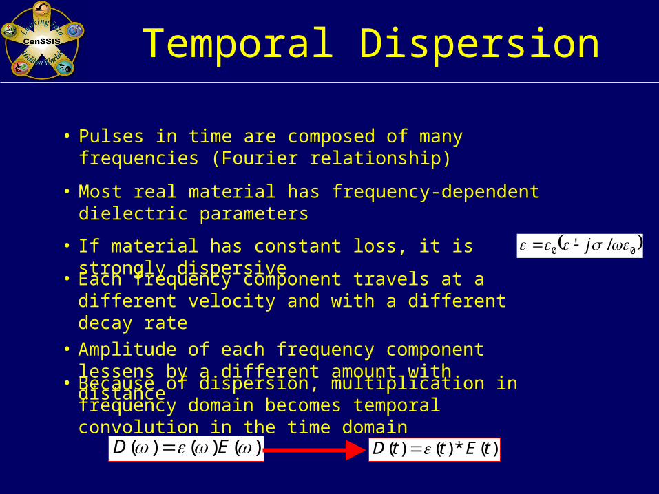
Temporal Dispersion
• Pulses in time are composed of many frequencies (Fourier relationship)
• Most real material has frequency-dependent dielectric parameters
00 /' j• If material has constant loss, it is strongly dispersive
• Each frequency component travels at a different velocity and with a different decay rate
• Amplitude of each frequency component lessens by a different amount with distance
)()()( ED )(*)()( tEttD
• Because of dispersion, multiplication in frequency domain becomes temporal convolution in the time domain

Dispersion of a Pulse 3 Fourier Components of Pulse at t0
• Each component travels at a different velocity (dispersion)
• Amplitude of component lessens in time (loss)
Same components at t>t0

Modeling Dispersion for Easy Transformation to Time
Domain
v
N
p p
p
j
A
100 1
'
N=2
Standard (2nd Order) Debye Model: simple form for complex permittivity, easily transformed to time domain differential equation
N
p p
p
j
A
12200
0
'
2
Lorentz Model: 2nd order when N = 1
01
100 1
'
jj
A
For 2202 / and A
[Cole-Cole Model is more accurate, not easily converted to time domain]
js
1
''' 00

1002222 '00
AjEjD pp 22
Lorentz
Conversion of Dispersion Models to Time Domain
110001010 1'11 jAjjjEjjD
Replace by D/E and multiply through by denominator
tj
Convert to time domain with
Et
EA
t
E
t
D
t
D
0011002
2
102
2
1 ''
Debye
tj
Convert to time domain with
EAt
E
t
ED
t
D
t
Dpp 1
2002
2
02
2
2
00''2'2

Modeling Dispersion for Easy Transformation to Time
Domain
Since Z-1 transforms to unit time delay, application to FDTD is simple
)()()(
)()(
ZEZZJ
ZEZD Av
)3()2()()(
)2
3()
2(
)()(
3210
1
ttEbttEbttEbtEb
ttJa
ttJ
tEtD Av
Z-Transform model keeps real permittivity constant, and
matches conductivity to measured values in terms of Z-1 [4 Zero Model]
’ = Constant, Z = e jt11
33
22
1102/1
1
Za
ZbZbZbbZ
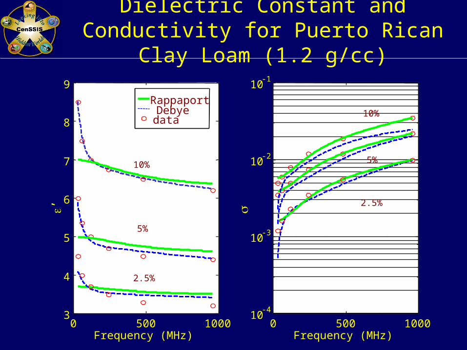
Frequency (MHz)0 500 1000
3
4
5
6
7
8
9
Frequency (MHz)
’
0 500 100010
-4
10-3
10-2
10-1
RappaportDebyedata
2.5%
5%
10%
2.5%
5%
10%
Dielectric Constant and Conductivity for Puerto Rican Clay Loam (1.2 g/cc)

7 7.5 8 8.5 9 9.5
0
10
20
30
40
50
60
Log Frequency
(1/m
)
7 7.5 8 8.5 9 9.5-3
-2.5
-2
-1.5
-1
-0.5
0
Log Frequency
- (
1/m
)
RappaportDebyedata
2.5%
5%
10%
2.5%
5%
10%
Real and Imaginary Wave Number for Puerto Rican Clay Loam (1.2g/cc)

Wave Propagation Variation as a Function of Clay Loam Moisture

Transverse Position (cm)
De
pth
(cm
)
Transmitter Receiver
Non-Metallic Mine
60 80 100 120 140 160 180
40
30
20
10
0
-10
-20
-30
-40
Rough Surface Test Geometry

0 1000 2000 3000 4000 5000 6000 7000 8000 9000 10000
-0.4
-0.3
-0.2
-0.1
0
0.1
0.2
0.3
0.4
Time (ps)
Re
lativ
e A
mp
litud
eNon-Metallic Mine Scattered Field 10
cm Deep - Smooth Surface
------- Air Dry Sand Non-Dispersive Loam 20% moistureDispersive Loam 20% moisture
++++++ooooooxxxxxx

0 1000 2000 3000 4000 5000 6000 7000 8000 9000 10000-0.4
-0.3
-0.2
-0.1
0
0.1
0.2
0.3
0.4
Time (ps)
Re
lativ
e A
mp
litud
eNon-Metallic Mine Scattered Field
(about 10 cm burial) - Rough Surface
------- Air Dry Sand Non-Dispersive Loam 20% moistureDispersive Loam 20% moisture
++++++ooooooxxxxxx

0 1000 2000 3000 4000 5000 6000 7000 8000 9000 10000-0.1
-0.05
0
0.05
0.1
Re
lativ
e A
mp
litud
e
0 1000 2000 3000 4000 5000 6000 7000 8000 9000 10000-0.04
-0.02
0
0.02
0.04
0.06
Time (ps)
Re
lativ
e A
mp
litud
e
Non-Dispersive Loam 20% moistureDispersive Loam 20% moisture
Non-Metallic Mine Scattered Field 10 cm depth a) Flat Surface, b) Rough Surface

80 cm
Square Target
Air
Soil d
11.28 cm
20 cm
60 cm
Circular Target
Air
Soil d
10 cm
20 cm
60 cm10 cm
80 cm
Sandy soil: s = 2.5, s = 0.01Target: m = 2.9, m = 0.004
Shape Determination of Buried Non-Metallic Targets, Multiple Single-Frequency
Observations

Different Buried Test Target Shapes
Heig
ht
(cm
)
Horizontal Position (cm)
-10 -5 0 5 10
-15
-10
-5
0Square
-20-10 -5 0 5 10
-15
-10
-5
0Circle
-20-10 -5 0 5 10
-15
-10
-5
0Diamond
-20
Blob
-10 -5 0 5 10
-15
-10
-5
0
-20-10 -5 0 5 10
-15
-10
-5
0Star
-20

Scattered Field - Real Part
500 MHz, depth = 5 cm
Horizontal Position (cm)
Heig
ht
(cm
)
-0.06
-0.04
-0.02
0
0.02
0.04
0.06
Circle
-40 -20 0 20 40-60
-40
-20
0
20
Diamond
-40 -20 0 20 40-60
-40
-20
0
20
Square
-40 -20 0 20 40-60
-40
-20
0
20
Star
-40 -20 0 20 40-60
-40
-20
0
20Blob
-40 -20 0 20 40-60
-40
-20
0
20

Scattered Field - Real Part
1000 MHz, depth = 5 cm
-0.2
-0.1
0
0.1
0.2
Horizontal Position (cm)
Heig
ht
(cm
)
Square
-40 -20 0 20 40-60
-40
-20
0
20Circle
-40 -20 0 20 40-60
-40
-20
0
20Diamond
-40 -20 0 20 40-60
-40
-20
0
20
Star
-40 -20 0 20 40-60
-40
-20
0
20Blob
-40 -20 0 20 40-60
-40
-20
0
20

Horizontal Position (cm)
Inte
nsi
ty
-40 -20 0 20 400
0.01
0.02
0.03
0.04
0.05
1000 MHz, depth = 5cm
square
circle
diamond
star
blob
-40 -20 0 20 400.02
0.025
0.03
0.035
0.04
500 MHz, depth = 5cm
square
circle
diamond
star
blob
Surface Field - Magnitude

Horizontal Position (cm)
-0.08-0.06-0.04-0.0200.020.04
Circle, r = 5.64 cm
Sandy Soil = 2.5, = 0.01freq = 500 MHz depth = 5 cm-20 0 20 40
0
-20
-40
-60-40
20
-20 0 20 40
0
-20
-40
-60
7.5 x 13.3 cm20
-40 -20 0 20 40
0
-20
-40
-60
5 x 20 cm20
-40 -20 0 20 40
0
-20
-40
-60
2.5 x 40 cm
-40
20
-20 0 20 40
0
-20
-40
-60
13.3 x 7.5 cm20
-40 -20 0 20 40
0
-20
-40
-60
20 x 5 cm20
-40 -20 0 20 40
0
-20
-40
-60
40 x 2.5 cm
-40
20
-20 0 20 40
0-20
-40
-60
10 x 10 cm20
-40
Heig
ht
(cm
)
Scattered Field - Aspect Ratio Dependence

Distinguishing Shapes of 3D Buried Objects under Rough Surfaces:
Geometry
Point Source
Rough Surface
Mine
10 cm
4 cm
5 cm
10 cm
Soil

Total Ex Field from an x-Directed Point Source, with a Buried Non-Metallic Square
Target
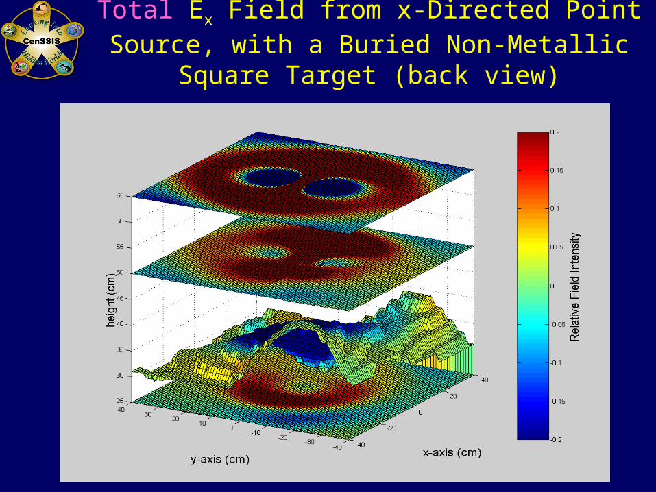
Total Ex Field from x-Directed Point Source, with a Buried Non-Metallic Square Target
(back view)

Comparison of Total Ex Field for Buried Non-Metallic Square and Circular
Targets

Comparison of Scattered Ex Field for Buried Non-Metallic Square and Circular
Targets

Soil Packing Affects Greatly Scattering: 3D FDFD with Short
Cylindrical Target
Relative Height 30
TNT in 26% moist Bosnian soil at 960 MHz

Transverse Position (cm)
Non-Metallic Target
Soil
Air
-20 -15 -10 -5 0 5 10 15 20
Dep
th (
cm)
-5
0
5
10
15
20
25
30
35
Surface Scattering Clutter Increases with Frequency. Example: 4 GPR Freq., PRCL 10%
moisture, 1.4 g/cc

Mine scattered field: smooth surface
Scattered field: rough surface with mine
Scattered field: rough surface only
Mine scattered field: rough surface
Display Format for each of Four Frequencies

480 MHz
Transverse Position (cm)
Dep
th (
cm)
Mine scattered field: smooth surface
-20 -10 0 10 20
0
10
20
30
-0.2
-0.1
0
0.1
0.2
Transverse Position (cm)
Dep
th (
cm)
Scattered field: rough surface with mine
-20 -10 0 10 20
0
10
20
30
-0.2
-0.1
0
0.1
0.2
Transverse Position (cm)
Dep
th (
cm)
Scattered field: rough surface only
-20 -10 0 10 20
0
10
20
30
-0.2
-0.1
0
0.1
0.2
Transverse Position (cm)
Dep
th (
cm)
Mine scattered field: rough surface
-20 -10 0 10 20
0
10
20
30
-0.2
-0.1
0
0.1
0.2
Am
plitu
de R
elative to Incid
ent
Am
plitu
de R
elative to Incid
ent
Am
plitu
de R
elative to Incid
ent
Am
plitu
de R
elative to Incid
ent

960 MHz
Transverse Position (cm)
Dep
th (
cm)
Mine scattered field: smooth surface
-20 -10 0 10 20
0
10
20
30
-0.2
-0.1
0
0.1
0.2
Transverse Position (cm)
Dep
th (
cm)
Scattered field: rough surface with mine
-20 -10 0 10 20
0
10
20
30
-0.2
-0.1
0
0.1
0.2
Transverse Position (cm)
Dep
th (
cm)
Scattered field: rough surface only
-20 -10 0 10 20
0
10
20
30
-0.2
-0.1
0
0.1
0.2
Transverse Position (cm)
Dep
th (
cm)
Mine scattered field: rough surface
-20 -10 0 10 20
0
10
20
30
-0.2
-0.1
0
0.1
0.2A
mp
litud
e Relative to In
ciden
tA
mp
litud
e Relative to In
ciden
t
Am
plitu
de R
elative to Incid
ent
Am
plitu
de R
elative to Incid
ent
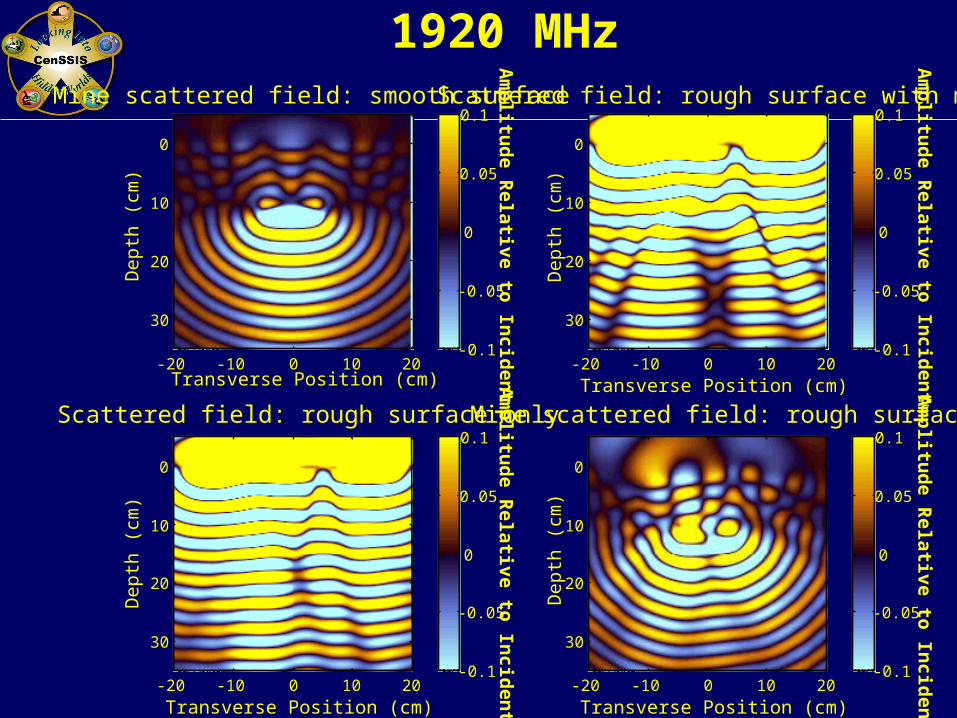
1920 MHz
Transverse Position (cm)
Dep
th (
cm)
Mine scattered field: smooth surface
-20 -10 0 10 20
0
10
20
30
-0.1
-0.05
0
0.05
0.1
Transverse Position (cm)
Dep
th (
cm)
Scattered field: rough surface with mine
-20 -10 0 10 20
0
10
20
30
-0.1
-0.05
0
0.05
0.1
Transverse Position (cm)
Dep
th (
cm)
Scattered field: rough surface only
-20 -10 0 10 20
0
10
20
30
-0.1
-0.05
0
0.05
0.1
Transverse Position (cm)
Dep
th (
cm)
Mine scattered field: rough surface
-20 -10 0 10 20
0
10
20
30
-0.1
-0.05
0
0.05
0.1A
mp
litud
e Relative to In
ciden
tA
mp
litud
e Relative to In
ciden
t
Am
plitu
de R
elative to Incid
ent
Am
plitu
de R
elative to Incid
ent

3840 MHz
Transverse Position (cm)
Dep
th (
cm)
Mine scattered field: smooth surface
-20 -10 0 10 20
0
10
20
30
-0.05
0
0.05
Transverse Position (cm)
Dep
th (
cm)
Scattered field: rough surface with mine
-20 -10 0 10 20
0
10
20
30
-0.05
0
0.05
Transverse Position (cm)
Dep
th (
cm)
Scattered field: rough surface only
-20 -10 0 10 20
0
10
20
30
-0.05
0
0.05
Transverse Position (cm)
Dep
th (
cm)
Mine scattered field: rough surface
-20 -10 0 10 20
0
10
20
30
-0.05
0
0.05
Am
plitu
de R
elative to Incid
ent
Am
plitu
de R
elative to Incid
ent
Am
plitu
de R
elative to Incid
ent
Am
plitu
de R
elative to Incid
ent

30o
Modulated Gaussian Pulse Plane Wave
AirAir
SoilSoil
Short Pulse GPR Interaction with Rough,
Dispersive Ground / Mine

From MineFacts, version 1.2, National Ground Intelligence Center
PMN-1A Non-Metallic AP Mine Geometry
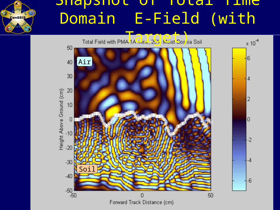
Air
Soil
Snapshot of Total Time Domain E-Field (with Target)

Soil
Air
Snapshot of Background Time Domain E-Field
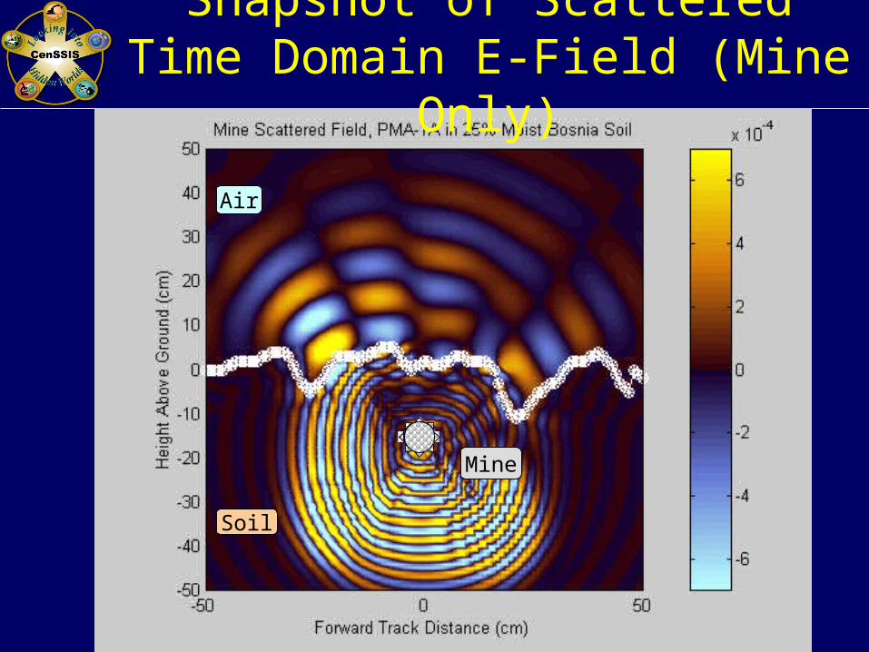
Soil
Air
Mine
Snapshot of Scattered Time Domain E-Field (Mine Only)

Rough Ground (cm)Rough Ground (cm)
Hei
gh
tH
eig
ht (c
m)
(cm
)
0-12
12
0
--
--24 24-48 48
Transmitter
Receiver
Effect of Rough Ground of Bistatic GPR Signals
0 100 200 300
-0.5
0
0.5
Time Step (Time Step (t = 20ps)t = 20ps)Sig
nal
Am
pli
tud
eS
ign
al A
mp
litu
de 0.5
-0.5
0.0
0.0 100 200 300
Mean Height variationMean Height variation hh= 6cm= 6cm
Correlation distance Correlation distance between surface between surface peakspeaks l lcc= 15cm= 15cm

Rough Ground Clutter Signal
Characterization
• Signals from rough ground vary considerably– Pulse shape depends on roughness and TR
position – Peak depends on particular TR position– Overall amplitude varies
• Monte Carlo simulation can model following relevant features– 2D FDTD model– Real measured impulse GPR excitation and
dispersive soil– 500 different rough surface realizations

Monte Carlo Analysis
• Run many simulations • Vary each run
– Change geometry– Change signal
• Compute statistics– Mean values – Standard deviations
• Conclude “typical” behavior– Determine likelihood of given test
• Set threshold and count number of occurrences of detection or false alarm --> ROC curve

Computational GeometryComputational Geometry
Z = 0
Z = 28cm
TransmitterTransmitter ReceiverReceiver24.5 cm
L = 294 cm
soilsoil minemine
Z = depth

Impulse Ground Impulse Ground Penetrating Radar Penetrating Radar
SpecificationsSpecifications
0 100 200 300
-4
-2
0
2
4
-4
-2
0
2
4
Time Step (Time Step (t=20ps)t=20ps)
Rel
ativ
e A
mp
litu
de
Rel
ativ
e A
mp
litu
de

Original Signal Averages Obscure Mine Signal
MineNo Mine
500 computed signals

Raw Signals
Cross-correlatewith reference
Shifting
Scaling
Shift and scale raw signals andtake average
Subtract shifted and scaled average from each raw signal
Compute different velocity in soil, shiftto line up the targetfeature
Physics-based Signal Processing flowchart

MineNo Mine
Ground Clutter Signal Removal

Realigning Signals to Presumed Mine Position
No Mine Mine

Average Mine Scattered Signals
h=3cm
h=1cm
lc=10cm lc=3cm

ROC Curves for Mismatched Target Depths
hh= 1cm = 1cm llcc= 10cm= 10cm
Trail depth=8.5cmTrail depth=8.5cm
test depth= 2.4cmtest depth= 2.4cm 3.6cm3.6cm 4.8cm4.8cm 6.1cm6.1cm 8.5cm8.5cm 9.8cm9.8cm
8.5
9.8
2.46.1
3.6
4.8

Water movement in a vertical column of a medium is described by the
advection-dispersion equation in the z-direction, as:
Where: = moisture contentz = depth [L] D = dispersion coefficient of water [L/t2]K = hydraulic conductivity [ L/t]t = time [t]
)())((
Kdz
d
dz
dD
dz
d
dt
d
Soil Moisture Change with Wetting

Moisture ProfileKsat = 0.2 cm/min
0.00
0.05
0.10
0.15
0.20
0.25
0 10 20 30 40 50 60Depth into Soil (cm)
Mo
istu
re C
on
ten
t (%
)
0.1 Minute
1 Minute
2 Minutes
3 Minutes
4 Minutes
Time Response Due to Saturating Soil Surface

Ground Surface
Source
Non-Metallic Target
Air
Soil with Varying Moisture Content
Testing geometry
-100 -80 -60 -40 -20 0 20 40 60 80 100
-100
-80
-60
-40
-20
0
20
40
60
Rough Surface with Buried Non Metallic Mine and Point Source
Geometry

Planar Ground Surface, 5% Uniform Moisture

Planar Ground Surface, 20% Uniform Moisture

Planar Ground Surface, 5 - 20% Moisture Profile

Rough Ground Surface, 5% Uniform Moisture

Rough Ground Surface, 20% Uniform Moisture

Rough Ground Surface, 5 - 20% Moisture Profile

Summary
• Realistic soil media complicates the sensing of subsurface objects– Loss affects penetration depth and makes surface
clutter more dominant– Rough interfaces produce additive uncertain
clutter and distort transmitted signals– Moisture variations cause huge propagation
differences
• Small contrast differences makes detection/ imaging more challenging
• Shapes of underground dielectric object are hard to distinguish
• Multistatic wideband GPR can provide much more information than monostatic