Submatrix maximum queries in Monge matrices and partial

Monge matrices, and their applications∗

Haim Kaplan† Shay Mozes‡ Yahav Nussbaum† Micha Sharir§

Abstract

We describe a data structure for submatrix maximum queries in Monge matrices or par-tial Monge matrices, where a query seeks the maximum element in a contiguous submatrixof the given matrix. The structure, for an n × n Monge matrix, takes O(n log n) space,O(n log2 n) preprocessing time, and answers queries in O(log2 n) time. For partial Mongematrices the space and preprocessing grow by α(n) (the inverse Ackermann function), andthe query remains O(log2 n). Our design exploits an interpretation of the column max-ima in a Monge (resp., partial Monge) matrix as an upper envelope of pseudo-lines (resp.,pseudo-segments).

We give two applications: (1) For a planar set of n points in an axis-parallel rectangleB, we build a data structure, in O(nα(n) log4 n) time and O(nα(n) log3 n) space, thatreturns, for a query point p, the largest-area empty axis-parallel rectangle contained inB and containing p, in O(log4 n) time. This improves substantially the nearly-quadraticstorage and preprocesing obtained by Augustine et al. [arXiv:1004.0558]. (2) Given an n-node arbitrarily weighted planar digraph, with possibly negative edge weights, we build, inO(n log2 n/ log log n) time, a linear-size data structure that supports edge-weight updates

and graph-distance queries between arbitrary pairs of nodes in O(n2/3 log5/3 n) time peroperation. This improves a previous algorithm of Fakcharoenphol and Rao [JCSS 72, 2006].Our data structure has already been applied in a recent maximum flow algorithm for planargraphs of Borradaile et al. [FOCS 2011].

1 Introduction

A matrix M is a Monge matrix if for every pair of rows i < j and every pair of columns k < ℓwe have Mik +Mjℓ ≤ Miℓ +Mjk; it is called an inverse Monge matrix if the reverse inequalityMik +Mjℓ ≥ Miℓ +Mjk holds for every such quadruple of indices.1 A typical situation whereMonge matrices arise is the following. Suppose we have two vertically ordered sets of points,

∗An extended abstract of this paper was presented at [34].†School of Computer Science, Tel Aviv University, Tel Aviv 69978, Israel. E-mail: haimk@post.tau.ac.il,

yahav.nussbaum@cs.tau.ac.il. Work by Haim Kaplan and Yahav Nussbaum were partially supported by Grant2006/204 from the U.S.–Israel Binational Science Foundation, by Grant 822/10 from the Israel Science Fund,and by the Israeli Centers of Research Excellence (I-CORE) program.

‡Department of Mathematics, Massachusetts Institute of Technology, Cambridge, MA 02139, USA. E-mail:shaym@mit.edu. Part of the work by Shay Mozes was conducted while at Brown University, and partiallysupported by NSF Grants CCF-0964037, CCF-1111109 and by a Kanellakis fellowship.

§School of Computer Science, Tel Aviv University, Tel Aviv 69978, Israel, and Courant Institute of Mathemati-cal Sciences, New York University, New York, NY 10012, USA. E-mail: michas@post.tau.ac.il. Work by MichaSharir was partially supported by NSF Grant CCR-08-30272, by Grant 2006/194 from the U.S.–Israel BinationalScience Foundation, by Grant 338/09 from the Israel Science Fund, and by the Hermann Minkowski–MINERVACenter for Geometry at Tel Aviv University.

1In what follows we will sometimes make no distinction between Monge and inverse Monge matrices. Notethat by reversing the order of the rows or of the columns, an inverse Monge matrix becomes a Monge matrix.

1

A and B, on the left and right vertical sides of an axis-parallel rectangle, respectively. Monge[43] observed that, for i < j and k < ℓ any path in the rectangle from point i of A to point ℓof B must cross any such path from point j of A to point k of B. It follows from the triangleinequality that the matrix in which the (i, k) entry stores the distance from point i of A to pointk of B has the Monge property. Consequently, Monge matrices proved to be useful in solvingproblems related to distances between points in the plane.

In addition, Monge matrices have many applications in combinatorial optimization andcomputational geometry: The traveling salesman problem can be solved in linear time if theunderlying cost matrix is a Monge matrix [51]. The greedy algorithm solves the trasportationproblem optimally if the costs form a Monge matrix [30]. Monge matrices were also usedto obtain efficient algorithms for several problems on convex n-gons, like finding the k furthestvertices from any vertex [2], finding a minimum-area circumscribing convex d-gon, and others [2,3]. For a survey on Monge matrices and their uses in combinatorial optimization see [12].

A particularly famous result with many applications is an algorithm by Aggarwal et al. [2]to find the minimum or the maximum in each row of an m×n Monge matrix in O(m+n) time.This algorithm is known as the SMAWK algorithm for the initials of its inventors. There arealso algorithms with slightly worse asymptotic running times for finding row maxima and rowminima in specific kinds of partial Monge matrices in which some of the entries are undefined[1, 36, 37]. In these cases we require that the matrix have the Monge property only with respectto the defined entries. We note that all of these algorithms actually assume the weaker propertyof total monotonicity of the underlying matrix (see below for the definition), which is impliedby the inverse Monge property.

1.1 Our contributions

We present a data structure for efficient submatrix maximum queries in an n×n Monge matrix.2

Our data structure is constructed in O(n log2 n) time, its size is O(n logn), and it can find themaximum in any (contiguous) submatrix, specified by a range of rows and a range of columns,in O(log2 n) time.

For the special case in which the query submatrix is a row-interval, that is, a contiguousportion of a single row, we present a data structure that requires O(n logn) preprocessing time,O(n logn) space, and can answer queries in O(logn) time. Note that when the query submatrixis a slab, that is, a contiguous subsequence of complete rows, it is easy to obtain a data structurethat can be constructed in O(n) time and can answer a query in O(1) time. We can achieve thatby computing row maxima using the SMAWK algorithm, and then constructing an interval-maxima data structure on the array of row-maxima. The range-maxima problem on an array iswell studied and several data structures with linear size, linear preprocessing time, and constantquery time are known ([28], see also [8] and the references therein).

We show how to extend our data structures to partial Monge matrices, which are Mongematrices that contain undefined entries, so that the defined entries form within each row andcolumn a contiguous interval (see, e.g., Figure 2). The query times of the submatrix max-imum, row-interval maximum, and slab maximum data structures all remain the same, buttheir sizes and construction times grow by a factor of α(n), except for the construction time ofthe row-interval data structure which grows by the slightly larger factor α(n) log n, and is nowO(nα(n) log2 n).

We obtain these data structures using techniques from computational geometry. Specifi-cally, we think of the rows of the matrix as tabulated functions over the discrete sequence of

2To simplify the presentation we discuss square matrices here. Our results apply also to rectangular matrices,see Section 3.

2

column indices, and exploit the fact that the Monge property implies that these functions arein fact discrete variants of pseudo-lines (or pseudo-segments in case of partial matrices). Thisconnection may prove useful for constructing other data structures for Monge matrices. Wedescribe our data structures in Section 3.

Our Monge row-interval maximum data structure has already been applied in a recentmaximum flow algorithm for planar graphs of Borradaile et al. [10]. In this paper we presenttwo new applications of our data structures. In the first application we give, for a planar pointset enclosed in some fixed axis-parallel box B, an almost linear-size structure for finding thelargest-area empty axis-parallel rectangle containing a query point, where the previous bestsolution required quadratic space. In the second application we substantially improve a datastructure of Fakcharoenphol and Rao [24] for distance queries in a dynamically weighted planardigraph when the edge weights can be negative. We elaborate on these two applications next.

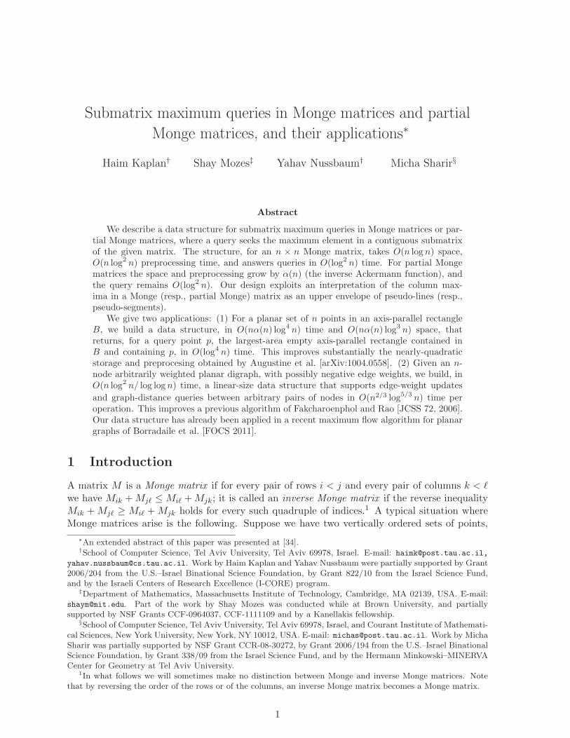
Finding the largest empty rectangle containing a query point. Let P be a set of npoints in a fixed axis-parallel rectangle B in the plane. A P -empty rectangle (or just an emptyrectangle for short) is any axis-parallel rectangle that is contained in B and its interior does notcontain any point of P . We consider the problem of preprocessing P into a data structure sothat, given a query point q, we can efficiently find the largest-area P -empty rectangle containingq. This problem arises, for example, in databases, for queries trying to identify ranges of valuesthat never appear together [27].

The largest-area P -empty rectangle containing q is amaximal empty rectangle, namely, it is aP -empty rectangle not contained in any other P -empty rectangle. Each side of a maximal emptyrectangle abuts a point of P or an edge of B. See Figure 1 for an illustration. Maximal emptyrectangles arise, among other applications, in the enumeration of “maximal white rectangles”in image segmentation [7].

B

q

Figure 1: A maximal P -empty rectangle containing a query point q.

Augustine et al. [6] gave a data structure for this problem whose storage and preprocessingtime are both O(n2 log n), and the query time is O(logn). In Section 4, we significantly improvethis result in terms of storage and preprocessing time. Specifically, we present a data structurethat requires O(nα(n) log3 n) space and can be constructed in O(nα(n) log4 n) time. Our querytime is O(log4 n), slightly worse than that of Augustine et al.

In a nutshell, our algorithm computes all the maximal P -empty rectangles and preprocessesthem into a data structure which is then searched with the query point. A major problemthat one faces is that the number of maximal P -empty rectangles can be quadratic in n (see,e.g., Figure 8), so we cannot afford to compute them explicitly. Instead, we exploit the inversepartial Monge matrix structure that exists in certain configurations of points (so-called “doublestaircases”), which facilitates a faster search for the maximum. The inverse Monge property of

3

areas of certain configurations of rectangles has been already observed in McKenna et al. [41]and used by Aggarwal and Suri [4] for finding the (global) P -empty rectangle of largest areaand the (global) P -empty rectangle of largest perimeter.

Our data structure can also be modified to find the largest-perimeter P -empty rectanglecontaining a given query point q.

Dynamic shortest path queries with negative edge weights in planar graphs. LetG be an n-node weighted directed planar graph, where the weights of the edges of G arearbitrary real numbers, possibly negative. In Section 5 we present a dynamic data structurethat can answer distance queries (that is, return the minimal path weight) between arbitrarypairs of nodes in G, and allows updates of edge weights. The time for a query or update isO(n2/3 log5/3 n). The construction time of our data structure is O(n log2 n/ log log n), and itrequires linear space. The bottleneck step in our construction is a single source shortest pathcomputation (when edges can have negative weights) [45]. We can also report the shortest pathQ itself in additional O(|Q| log log∆) time, where ∆ is the maximum degree of a node in thepath Q.

Our data structure is based on the data structure of Fakcharoenphol and Rao [24], whichhas O(n4/5 log13/5 n) query time and requires O(n logn) space, and on the data structure ofKlein [38], which has the same query time and space bound as our algorithm but does notsupport negative edge weights. For the convenience of the reader, we provide a review of thesetechniques before adapting and extending them to our setup.

Italiano et al. [32] extended the data structure of Klein to allow insertions and deletionsof edges that do not change the embedding of the graph. This technique also applies to ourdata structure, and we can extend it to support insertions and deletions of edges, retaining thesame asymptotic time bounds for updates (including insertions, deletions, and changes of edgeweights) and queries, as well as the aforementioned bounds on storage and preprocessing.

1.2 Related work

As we mentioned the range-maxima problem on an array is well studied and several datastructures with linear size, linear preprocessing time, and constant query time were developedfor it. The range-maxima problem on general multidimensional arrays has also been studied, andthe best data structure of Yuan and Atallah [53] is linear in the size of the matrix (i.e. O(n2)),can be constructed in O(n2) time, and answers a query in constant time. Brodal et al. [11]proved that with n2/c additional bits a query must take Ω(c) time. In contrast, our resultsshow that on matrices with the Monge property the range minima problem is substantiallyeasier.

Largest empty rectangles. The problem of finding the largest empty rectangle containinga query point was introduced in the paper mentioned above by Augustine et al. [6]. An easierproblem that has been studied more extensively is that of finding the largest-area P -empty axis-parallel rectangle contained in B. Notice that the largest P -empty square is easier to compute,because its center is a Voronoi vertex in the L∞-Voronoi diagram of P (and of the edges of B),which can be found in O(n logn) time [19, 39]. There have been several studies on finding thelargest-area maximal empty rectangle [5, 16, 46, 21, 49] in B; the fastest algorithm to date, byAggarwal and Suri [4], takes O(n log2 n) time and O(n) space. We use many of the observationsin these algorithms, most important of which is the quadratic number of maximal rectanglesgenerated by two “parallel” monotone chains of points, and the inverse Monge property which

4

they satisfy. Our main contribution is in adapting these ideas to construct a data structure forfinding the largest empty rectangle containing a query point.

Nandy et al. [47] show how to find the largest-area axis-parallel empty rectangle avoiding aset of polygonal obstacles in O(n log2 n) time and O(n) space. Boland and Urrutia [9] presentan algorithm for finding the largest-area axis-parallel rectangle inside an n-sided simple polygonin O(n logn) time. Chaudhuri et al. [15] give an algorithm to find the largest-area P -emptyrectangle, with no restriction on its orientation, in O(n3) time.

The problem can be studied for regions other than axis-parallel rectangles. Augustine etal. [6] also studied the case where the regions containing the query point are disks. For thiscase they gave a data structure that requires O(n2) space, O(n2 log n) preprocessing time, andcan answer a query in O(logn) time.3

Distance queries in planar graphs. Static data structures that preprocess an input planargraph to answer distance queries efficiently were studied by many authors [13, 18, 22, 24, 25,26, 38, 44, 48]. The dynamic setting in which updates of edge weights are supported wasrecently studied by Fakcharoenphol and Rao [24]. They describe a data structure that supportsonly non-negative edge weights, requires O(n logn) space, O(n log3 n) preprocessing time, andperforms a query or update in O(n2/3 log7/3 n) time. They also gave a data structure thatsupports negative edge weights but with query and update time of O(n4/5 log13/5 n), with thesame space and preprocessing time. Klein [38], using the technique of Fakcharoenphol and Rao,gave a simpler data structure for the case of non-negative edge weights that requires linearsize, O(n logn) preprocessing time, and O(n2/3 log5/3 n) time per query and update. Our datastructure is based on these results of Fakcharoenphol and Rao and of Klein.

2 Preliminaries

Totally monotone and Monge matrices. A matrix M is totally monotone if, for every pairof rows i < j and every pair of columns k < ℓ, Mik < Miℓ implies Mjk < Mjℓ. The SMAWKalgorithm of Aggarwal et al. [2] finds all row maxima in a totally monotone m × n matrix inO(m + n) time. By negating the entries of the matrix and reversing the order of the columnsto recover total monotonicity, we obtain a totally monotone matrix in which the maximum ofeach row is the negation of the minimum entry of the row in the original matrix. By applyingthe SMAWK algorithm to the transformed matrix we can also find the row minima in a totallymonotone m× n matrix in O(m+ n) time.

A matrix M is a Monge matrix (also called concave Monge matrix) if for every pair of rowsi < j and every pair of columns k < ℓ we have Mik + Mjℓ ≤ Miℓ + Mjk. A matrix M is aninverse Monge matrix (also called convex Monge matrix) if for every pair of rows i < j andevery pair of columns k < ℓ we have Mik + Mjℓ ≥ Miℓ + Mjk. Clearly if M is Monge (resp.,inverse Monge) then so is its transpose M t. It is easy to verify that if M is an inverse Mongematrix, then M and M t are totally monotone. Also, if M is a Monge matrix, then by negatingthe entries of M , or by reversing the order of the rows or of the columns, we get an inverseMonge matrix. Therefore, we can use the SMAWK algorithm for finding, in linear time, rowmaxima, row minima, column maxima and column minima in a Monge matrix or in an inverseMonge matrix.

We say that a matrix M is a partial matrix if some of the entries of M are undefined,but the defined entries of each row are continuous, and the defined entries of each column are

3In [35], Kaplan and Sharir have recently improved the storage and preprocessing costs to nearly linear in n.

5

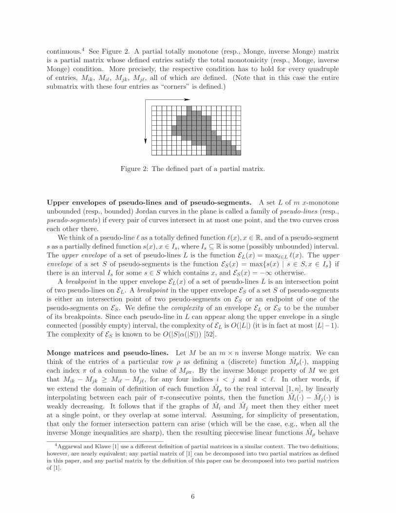
continuous.4 See Figure 2. A partial totally monotone (resp., Monge, inverse Monge) matrixis a partial matrix whose defined entries satisfy the total monotonicity (resp., Monge, inverseMonge) condition. More precisely, the respective condition has to hold for every quadrupleof entries, Mik, Miℓ, Mjk, Mjℓ, all of which are defined. (Note that in this case the entiresubmatrix with these four entries as “corners” is defined.)

Figure 2: The defined part of a partial matrix.

Upper envelopes of pseudo-lines and of pseudo-segments. A set L of m x-monotoneunbounded (resp., bounded) Jordan curves in the plane is called a family of pseudo-lines (resp.,pseudo-segments) if every pair of curves intersect in at most one point, and the two curves crosseach other there.

We think of a pseudo-line ℓ as a totally defined function ℓ(x), x ∈ R, and of a pseudo-segments as a partially defined function s(x), x ∈ Is, where Is ⊆ R is some (possibly unbounded) interval.The upper envelope of a set of pseudo-lines L is the function EL(x) = maxℓ∈L ℓ(x). The upperenvelope of a set S of pseudo-segments is the function ES(x) = maxs(x) | s ∈ S, x ∈ Is ifthere is an interval Is for some s ∈ S which contains x, and ES(x) = −∞ otherwise.

A breakpoint in the upper envelope EL(x) of a set of pseudo-lines L is an intersection pointof two pseudo-lines on EL. A breakpoint in the upper envelope ES of a set S of pseudo-segmentsis either an intersection point of two pseudo-segments on ES or an endpoint of one of thepseudo-segments on ES . We define the complexity of an envelope EL or ES to be the numberof its breakpoints. Since each pseudo-line in L can appear along the upper envelope in a singleconnected (possibly empty) interval, the complexity of EL is O(|L|) (it is in fact at most |L|−1).The complexity of ES is known to be O(|S|α(|S|)) [52].

Monge matrices and pseudo-lines. Let M be an m × n inverse Monge matrix. We canthink of the entries of a particular row ρ as defining a (discrete) function Mρ(·), mappingeach index π of a column to the value of Mρπ. By the inverse Monge property of M we getthat Mik − Mjk ≥ Miℓ − Mjℓ, for any four indices i < j and k < ℓ. In other words, if

we extend the domain of definition of each function Mρ to the real interval [1, n], by linearlyinterpolating between each pair of π-consecutive points, then the function Mi(·) − Mj(·) isweakly decreasing. It follows that if the graphs of Mi and Mj meet then they either meetat a single point, or they overlap at some interval. Assuming, for simplicity of presentation,that only the former intersection pattern can arise (which will be the case, e.g., when all theinverse Monge inequalities are sharp), then the resulting piecewise linear functions Mρ behave

4Aggarwal and Klawe [1] use a different definition of partial matrices in a similar context. The two definitions,however, are nearly equivalent; any partial matrix of [1] can be decomposed into two partial matrices as definedin this paper, and any partial matrix by the definition of this paper can be decomposed into two partial matricesof [1].

6

Column ℓ

Row i

Row j

Column k

Figure 3: The pseudo-lines of two rows i < j in an inverse Monge matrix.

as pseudo-lines.5 Moreover, for i < j, the pseudo-line of row i lies above the pseudo-line of rowj to the left of their intersection point, and this order is reversed to the right of that point; veryinformally, the “slopes” of the pseudo-lines of the rows are arranged in increasing order. SeeFigure 3. Note that the same analysis applies to Monge matrices, except that the order of the“slopes” of the resulting pseudo-lines is decreasing.

Similarly if M is an m × n partial inverse Monge matrix then, since the defined entries ineach row are consecutive, we can think of each row as a discrete partially defined function,which, after being interpolated in the same manner as above, is defined over some connectedsubinterval of [1, n]. By the inverse Monge property we get that Mik −Mjk ≥ Miℓ −Mjℓ, wheni < j, k < ℓ, and these four entries of M are all defined. Therefore the interpolated partialfunctions corresponding to the rows of M form a family of pseudo-segments.

3 The data structure

In this section we develop the main result of our paper, namely, data structures for submatrixmaximum queries in (inverse) Monge matrices and in partial (inverse) Monge matrices.

The model that we assume, which is the same model used by all the previous studies men-tioned in the introduction, is that the input matrix M is not given explicitly—it has too manyentries. Instead, it is given implicitly so that one can retrieve any desired entry Mij of M inO(1) time.

3.1 Submatrix maximum in (inverse) Monge matrices

Let M be an m× n inverse Monge matrix and consider the interpretation of the rows of M aspseudo-lines (see Section 2). The upper envelope E of the rows of M consists of the columnmaxima of M . An explicit representation of the entire upper envelope requires O(n) values.However, the envelope E contains only O(m) breakpoints, and we use these breakpoints toimplicitly represent E .6 We will use this compact representation for upper envelopes of severalsubsets of the rows, and we note that the saving becomes significant when the number of rowsis significantly smaller than the number of columns.

The breakpoints of E partition the domain [1, n] into intervals, so that E is attained by asingle pseudo-line (i.e., row) over each interval. Every column π is contained in one of theseintervals, and we can find that interval using binary search on the breakpoints. Once we found

5In fact it suffices that M t is totally monotone for the functions Mρ to behave as pseudo-lines.6Technically, since we are dealing with discrete versions of pseudo-lines, a breakpoint occurs in general “be-

tween” two consecutive columns. The representation of breakpoints is handled accordingly, but all that reallycounts is the pair of consecutive columns between which the breakpoint appears. We will not refer to this issueexplicitly in what follows.

7

the interval, we know which pseudo-line attains E at π (that is, which row contains the maximumof column π), and can then retrieve that maximum in O(1) time. We conclude that we can findthe maximum in a column π of M in O(logm) time, given the implicit representation of E asa list of its breakpoints, and of the the pseudo-line (row) that attains E between each pair ofconsecutive breakpoints.

We find the implicit representation of the upper envelope of all pseudo-lines in O(m(logm+log n)) time using the following standard divide-and-conquer approach. We build a balancedbinary tree Th over the rows of M . For each node u of Th we compute the upper envelope of thepseudo-lines representing the rows in the subtree rooted at u (which we call the upper envelopeof u for short). The upper envelope of a leaf is trivial, since it represents a single row, and nocomputation is needed. For an internal node u, we construct its upper envelope by merging theenvelopes of its two children w1 and w2, where w1 is the child whose rows have lower indices.(This is similar to the hierarchical representation of an upper envelope used by Overmars andvan-Leeuwen to support insertions and deletions of lines [50].)

Let k be the number of rows at the leaves of the subtree of Th rooted at u. The number ofbreakpoints in each of the upper envelopes of u, w1, and w2 is O(k). By the total monotonicityof M t and its implications discussed above, the upper envelope of u starts with a prefix of theupper envelope of w1, reaches a breakpoint between the pseudo-line of some row of w1 and thatof some row of w2, and ends with a suffix of the upper envelope of w2. We merge the sequencesof breakpoints of the envelopes of w1 and of w2, checking at each breakpoint, in O(1) time, forthe relative order of the envelopes over it, and keeping the breakpoint only if it remains on theupper envelope of u. This allows us to find the interval containing the unique intersection of theenvelopes. Over this interval there are only two rows, one from each subtree, “competing” forthe maximum, and we find the intersection point of their pseudo-lines in O(logn) time. Thenwe form the new envelope of u as prescribed above, by concatenating the prefix of the upperenvelope of w1, the new breakpoint, and the suffix of the upper envelope of w2. All these stepstake O(k + log n) time. Summing these costs over all nodes of Th, we get an overall cost ofO(m(logm+ logn)). The total size of Th is O(m logm).7

We use the tree Th to create a data structure for reporting the maximum of a column withina given range of consecutive rows. A query in this data structure is a column π and a rangeof rows [ρ, ρ′], and the output is the maximum entry of M at column π between rows ρ and ρ′

(inclusive). We answer such a query as follows. There are O(logm) canonical nodes of Th whosesets of rows are disjoint and cover [ρ, ρ′]. (The set of rows of each such node u is contained in[ρ, ρ′], but the set of rows of the parent of u is not.) For each such canonical node u, we locatethe interval of the envelope of u containing π, and hence the maximum of column π among therows of u. The output is the largest of these O(logm) maxima. A binary search within eachenvelope takes O(logm) time, and therefore the total query time is O(log2m).

We can reduce the query time by a logarithmic factor using fractional cascading [17]. Thistechnique allows us to insert bridges from the envelope of a node u of Th to the envelopes ofits two children, such that once we locate the interval containing column π in the envelope ofu, we can locate the interval containing column π in the envelope of its children in O(1) time.This construction does not incur (asymptotically) any space or preprocessing time overhead,

7We could, in fact, construct Th in O(m log n) time and represent it using only O(m) space at the cost ofsomewhat complicating the algorithm. For that we have to do a binary search to locate the last breakpoint ofthe envelope of w1 which is also on the envelope of u and the first breakpoint of the envelope of w2 which is onthe envelope of u. To avoid copying parts of the envelopes of w1 and w2 in order to produce the envelope of u werepresent envelopes using persistent search trees and produce the envelope of u by splitting and concatenatingnondestructively the search trees representing the envelopes of w1 and w2 in O(log k) time and extra space [23].We do not know how to efficiently combine these persistent search trees with fractional cascading which we useto speed up the query.

8

but reduces the query time to O(logm).Note that for this data structure we only used the fact that M t is a totally monotone matrix

(see a comment made earlier). Therefore, by transposing the matrix, we get the row-intervalmaximum data structure for a totally monotone matrix:

Lemma 3.1. Given a totally monotone matrix of size m×n, one can construct, in O(n(logm+log n)) time, a data structure of size O(n logn) that can report the maximum entry in a queryrow and a range of columns in O(log n) time.

We note that by a symmetric treatment of the lower envelope of pseudo-lines we can con-struct a variant of the data structure that reports minima rather than maxima.

We continue now to construct a data structure that answers maximum queries within asubmatrix of M . We build the tree Th over the rows of M , with an upper envelope for eachnode of Th, in O(m(logm+logn)) time as before. We also construct, in O(n(logm+logn)) time,the symmetric row-interval maximum data structure of Lemma 3.1 for finding the maximumelement of a row within a consecutive range of columns, and denote it by B; A query in B takesO(logn) time. For every node u of Th we find and store the maximum in every interval of theupper envelope of u by an appropriate query to B.

There are O(m logm) such intervals in all nodes of Th, but each such interval may appearin the upper envelope of more than one node of Th. In fact, if we recall the construction ofTh then we can easily verify that there are only O(m) distinct such intervals in all the upperenvelopes of the nodes of Th together. The reason for that is that when we merge the upperenvelopes of the children w1 and w2 of a node u then at most two new intervals are created inthe upper envelope of u. All other intervals in the upper envelope of u appear also either in theupper envelope of w1 or in the upper envelope of w2.

It follows that we can find the maxima in each of these intervals, when it is created, in a totalof O(m logn) time. For every node u of Th we build a range maximum query data structureover the maxima of the intervals of the upper envelope of u. For our purpose it is sufficientto use a binary search tree over these intervals, augmented with subtree maxima stored at itsnodes, which can answer a range maximum query in O(logm) time. Later on, in Section 3.3,we will use the more sophisticated structure of [8] for another variant of our data structure.

A query in this data structure is a submatrix of M with specified ranges R of consecutiverows and C of consecutive columns, and the answer is the maximum entry in this submatrix.To answer such a query, we first represent R as the (disjoint) union of O(logm) subtrees of Th.For each root u of such a subtree, we find the maximum of the upper envelope of u in the rangedefined by C as follows; refer to Figure 4. We find the set I of consecutive intervals of the upperenvelope of u that are fully contained in C. Then we find the maximum in the range coveredby the union of the intervals in I using the range maximum data structure that we have builtover the intervals of the envelope of u. The prefix p of C which is not covered by I is containedin a single interval of the upper envelope of u. Therefore, the maximum of the upper envelopeof u within p is in a specific row ρ. Similarly the maximum of the upper envelope of u in thesuffix s of C not covered by I is attained at a specific row ρ′. We use the structure B to find themaximum in row ρ within column range p, and the maximum in row ρ′ within column ranges. Repeating this step for each of the O(logm) subtrees of Th that comprise R, we cover theentire query submatrix. The cost of finding the maximum in the upper envelope over C of anysingle node u of Th is O(logm+logn), so the overall query time is O(logm(logm+logn)). Wethus obtain the following submatrix maximum data structure:

Theorem 3.2. Given an inverse Monge matrix8 of size m × n, one can construct in O((m +

8This theorem in fact holds for any totally monotone matrix whose transpose is also totally monotone.

9

C

p s

envelopeat u

u

I

Figure 4: Maximum query at a single node u of Th.

n)(logm+log n)) time a data structure of size O(m logm+n logn) that can report the maximumentry in any query submatrix in O(logm(logm+ log n)) time.

Again, we can construct a variant of this data structure for finding minima instead of maximawithin the same time bounds. The same results also apply to Monge matrices.

3.2 Submatrix maximum in partial Monge matrices

We extend the two data structures from the previous section to partial inverse Monge matrices.LetM denote an m×n partial inverse Monge matrix, and consider the interpretation of the rowsof M as pseudo-segments. Since the complexity of the upper envelope of k pseudo-segmentsis O(kα(k)) [52], it follows that there are O(kα(k)) breakpoints in the upper envelope of anysubset of k rows.

We use again a divide-and-conquer approach, but this time merging the upper envelopes ofthe two children w1, w2 of a node u of Th is slightly more involved, since the envelopes maycross each other multiple times. To merge the envelopes, we first merge the lists of break-points, keeping only those that appear on the envelope of u, each new interval can containa new breakpoint of the upper envelope at u. Intervals of this kind are characterized by theproperty that the envelope of u is attained at their left (resp., right) endpoint by the envelopeof the left (resp., right) child of u. We find the new breakpoint inside each such interval inO(logn) time, and complete the construction of the envelope at u in a similar manner to theone described in the previous section. Since we pay O(logn) time to find a new breakpoint,and there are O(mα(m) logm) breakpoints in total (over all nodes of the tree), the constructiontakes O(mα(m) logm log n) time, and the required storage is O(mα(m) logm). The query time(with fractional cascading) remains O(logm).

An alternative approach is to apply Hershberger’s algorithm [29], which constructs the upperenvelope of k segments in O(k log k) time. The algorithm is also applicable to the case at handof pseudo-segments, and, as above, we incur the extra factor O(log n) for finding the intersectionof two pseudo-segments. However, since we need to construct an entire hierarchy of envelopes,Hershberger’s algorithm does not make the whole procedure more efficient.

Again, by applying the algorithm described above to M t, we get the following row-intervalmaximum data structure:

10

Lemma 3.3. Given a partial totally monotone matrix of size m × n, one can construct, inO(nα(n) logm log n) time, a data structure of size O(nα(n) log n) that can report the maximumentry in a query row and a contiguous range of columns in O(logn) time.

We next develop the submatrix maximum data structure. Similar to what was done be-fore, we construct the tree Th and the row-interval maxima data structure B, but this timethe construction takes O((mα(m) + nα(n)) logm log n) time. Since the overall number ofbreakpoints in the upper envelopes of the nodes of Th is now O(mα(m) logm), the total timefor finding the maximum in every interval between two consecutive breakpoints, over all en-velopes, is now O(mα(m) logm log n). Therefore, the total construction time is O((mα(m) +nα(n)) logm log n), and the total size for the data structure is O(mα(m) logm + nα(n) log n).The rest of the data structure is constructed exactly as in the case of full matrices, and thequery time remains O(logm(logm+ logn)).

In conclusion, we get the following submatrix maximum data structure for partial matrices:

Theorem 3.4. Given a partial inverse Monge matrix9 one can construct, in O((mα(m) +nα(n)) logm log n) time, a data structure of size O(mα(m) logm+ nα(n) log n) that can reportthe maximum entry in a query submatrix in O(logm(logm+ log n)) time.

Again, the same results apply for partial Monge matrices. As in Section 3.1, we can alsoapply symmetric variants of the above constructions for answering submatrix minimum queries.

3.3 Maximum in a consecutive range of rows

As mentioned in Section 1.1, in the special case where the query submatrices consist of con-tiguous ranges of complete rows (i.e., with the entire range of columns), we can produce a moreefficient slab maximum data structure. Specifically, we find the maximum in each row usingthe SMAWK algorithm [2], and then construct in linear time a data structure that answersrange maximum queries on contiguous ranges of the row maxima, in O(1) time; see [8] and thereferences therein.

Theorem 3.5. Given a totally monotone matrix of size m×n, one can construct, in O(m+n)time, a data structure of size O(m) that can report the maximum entry in a query set of completeconsecutive rows, in O(1) time.

For the case of partial totally monotone matrices we can construct a similar data structureusing the algorithm of Klawe and Kleitman [37] for finding row maxima instead of the SMAWKalgorithm.10 This yields:

Theorem 3.6. Given a partial totally monotone matrix of size m × n, one can construct, inO(nα(m) + m) time, a data structure of size O(m) that can report the maximum entry in aquery range of consecutive rows, in O(1) time.

4 Maximal empty rectangle containing a query point

Let P be a set of n points inside an axis-parallel rectangular region B in the plane. In this sectionwe present the first application of our data structures, which is an algorithm that preprocesses P

9As Theorem 3.2, this theorem also holds for any partial totally monotone matrix whose transpose is alsototally monotone.

10The definition of partial matrices in [37] is the one in [1], which is different than the definition used in thispaper. However, the algorithm of [37] does apply in our case since, as previously noted, we can decompose apartial matrix into two partial matrices in the sense of [37] and run the algorithm of [37] on each of the twomatrices.

11

into a data structure, so that, given a query point q ∈ B, we can efficiently find the largest-areaaxis-parallel P -empty rectangle containing q and contained in B. We refer the reader to theintroduction for the notation that we shall use here.

We assume that the points of P are in general position, so that (i) no two points have thesame x-coordinate or the same y-coordinate, and (ii) all the maximal P -empty rectangles havedistinct areas.

One of the auxiliary structures that we use is a two-dimensional segment tree. This datastructure can store a setM of N axis-parallel rectangles in the plane, such that we can efficientlyreport all rectangles, or just find the largest rectangle, containing a query point. Here is a briefreview of the structure, provided for the sake of completeness. Let M be a set of N axis-parallelrectangles in the plane. In our case these N rectangles will be maximal P -empty rectangles, asdefined in the introduction; they are therefore defined by n points so their x-projections andtheir y-projections have only n distinct endpoints. We first construct a standard segment treeS [20] on the x-projections of the rectangles in M. This is a balanced binary search tree whoseleaves correspond to the O(n) intervals between consecutive endpoints of the x-projections of therectangles. The span of a node v is the minimal interval containing all intervals correspondingto the leaves of its subtree. Every rectangle R ∈ M is stored at each node v such that thex-projection of R contains the span of v but does not contain the span of the parent of v. Thetree has O(n) nodes, each rectangle is stored at O(log n) nodes, and the size of the structure isthus O(N log n). All the rectangles containing a query point q must be stored at the nodes onthe search path of the x-coordinate of q in the tree.

For each node u of S we take the set Mu of rectangles stored at u, and construct a secondarysegment tree Su, storing the y-projections of the rectangles ofMu in the same manner. The totalsize and the preprocessing time of the resulting two-dimensional segment tree is O(N log2 n).We can retrieve all rectangles containing a query point q by traversing the search path π of(the x-coordinate of) q in the primary tree, and then by traversing the search paths of (they-coordinate of) q in each of the secondary trees associated with the nodes along π. Therectangles stored at the secondary nodes along these paths are exactly those containing q. Ifwe store at each secondary node only the rectangle of largest area among those assigned tothat node, we can easily find the largest-area rectangle of M containing a query point, in timeO(log2 n). Storing only one rectangle at each secondary node reduces the size of the segmenttree to O(N logn), but the preprocessing time remains O(N log2 n).

A simple-minded solution would just takeM to be the set of all maximal P -empty rectangles.Unfortunately, this may not be efficient since the size N of M could be quadratic in n in theworst case. (See Figure 8 for an illustration.) To get an efficient solution we will store only asubset of the rectangles of cardinality nearly linear in n, in a two-dimensional segment tree, andfor the other rectangles we will use an additional, implicit representation. For this purpose wewill decompose our problem into subproblems so that in each of the subproblems most of themaximal empty rectangles can be represented in a partial inverse Monge matrix, and we will useour submatrix maximum query data structure on the resulting matrix to find the largest-areaP -empty rectangle containing any query point q.

4.1 Maximal rectangles with edges on the boundary of B

Let et, eb, eℓ, and er be the top, bottom, left, and right edges of B, respectively. Naamadet al. [46] classified the maximal P -empty rectangles within B according to the number oftheir edges that touch the edges of B. They show that there are only O(n) maximal P -emptyrectangles with at least one edge on ∂B. We precompute these rectangles and store them ina two-dimensional segment tree S, as described above. At query time we find the rectangle

12

of largest area among those special “anchored” rectangles that contain the query point q, bysearching with q in S. (The segment tree S will also store additional rectangles that will arisein later steps of the construction, but the overall number of these rectangles will still be nearlylinear; see below for details.)

For the sake of completeness, we provide the easy details concerning the number of theseanchored maximal P -empty rectangles and their construction cost.

(i) Three edges of R lie on ∂B. It is easy to verify that there are only four such rectangles,one for each triple of edges of B.

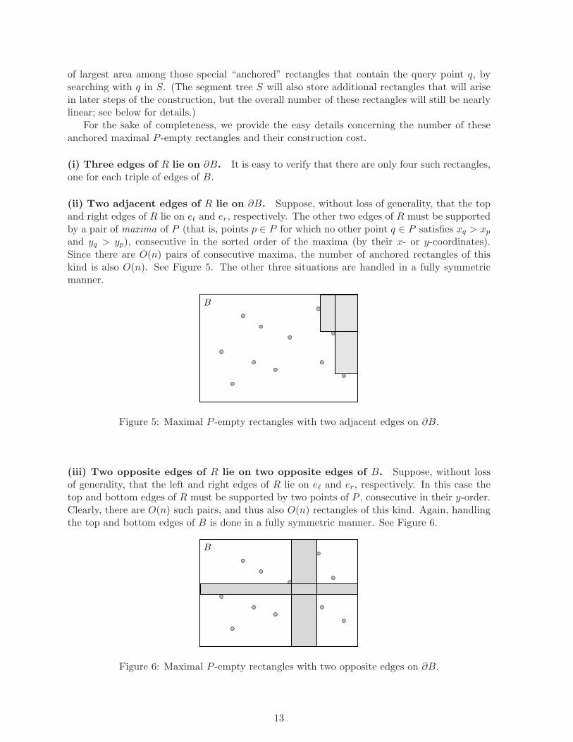
(ii) Two adjacent edges of R lie on ∂B. Suppose, without loss of generality, that the topand right edges of R lie on et and er, respectively. The other two edges of R must be supportedby a pair of maxima of P (that is, points p ∈ P for which no other point q ∈ P satisfies xq > xpand yq > yp), consecutive in the sorted order of the maxima (by their x- or y-coordinates).Since there are O(n) pairs of consecutive maxima, the number of anchored rectangles of thiskind is also O(n). See Figure 5. The other three situations are handled in a fully symmetricmanner.

B

Figure 5: Maximal P -empty rectangles with two adjacent edges on ∂B.

(iii) Two opposite edges of R lie on two opposite edges of B. Suppose, without lossof generality, that the left and right edges of R lie on eℓ and er, respectively. In this case thetop and bottom edges of R must be supported by two points of P , consecutive in their y-order.Clearly, there are O(n) such pairs, and thus also O(n) rectangles of this kind. Again, handlingthe top and bottom edges of B is done in a fully symmetric manner. See Figure 6.

B

Figure 6: Maximal P -empty rectangles with two opposite edges on ∂B.

13

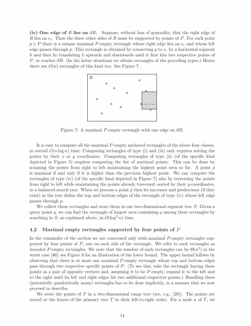
(iv) One edge of R lies on ∂B. Suppose, without loss of generality, that the right edge ofR lies on er. Then the three other sides of R must be supported by points of P . For each pointp ∈ P there is a unique maximal P -empty rectangle whose right edge lies on er and whose leftedge passes through p. This rectangle is obtained by connecting p to er by a horizontal segmenth and then by translating h upwards and downwards until it first hits two respective points ofP , or reaches ∂B. (In the latter situations we obtain rectangles of the preceding types.) Hencethere are O(n) rectangles of this kind too. See Figure 7.

B

Figure 7: A maximal P -empty rectangle with one edge on ∂B.

It is easy to compute all the maximal P -empty anchored rectangles of the above four classes,in overall O(n logn) time: Computing rectangles of type (i) and (iii) only requires sorting thepoints by their x or y coordinates. Computing rectangles of type (ii) (of the specific kinddepicted in Figure 5) requires computing the list of maximal points. This can be done byscanning the points from right to left maintaining the highest point seen so far. A point pis maximal if and only if it is higher than the previous highest point. We can compute therectangles of type (iv) (of the specific kind depicted in Figure 7) also by traversing the pointsfrom right to left while maintaining the points already traversed, sorted by their y-coordinates,in a balanced search tree. When we process a point p then its successor and predecessor (if theyexist) in the tree define the top and bottom edges of the rectangle of type (iv) whose left edgepasses through p.

We collect these rectangles and store them in our two-dimensional segment tree S. Given aquery point q, we can find the rectangle of largest area containing q among these rectangles bysearching in S, as explained above, in O(log2 n) time.

4.2 Maximal empty rectangles supported by four points of P

In the remainder of the section we are concerned only with maximal P -empty rectangles sup-ported by four points of P , one on each side of the rectangle. We refer to such rectangles asbounded P -empty rectangles. We note that the number of such rectangles can be Θ(n2) in theworst case [46]; see Figure 8 for an illustration of the lower bound. The upper bound follows byobserving that there is at most one maximal P -empty rectangle whose top and bottom edgespass through two respective specific points of P . (To see this, take the rectangle having thesepoints as a pair of opposite vertices and, assuming it to be P -empty, expand it to the left andto the right until its left and right edges hit two additional respective points.) Handling these(potentially quadratically many) rectangles has to be done implicitly, in a manner that we nowproceed to describe.

We store the points of P in a two-dimensional range tree (see, e.g., [20]). The points arestored at the leaves of the primary tree T in their left-to-right order. For a node u of T , we

14

B

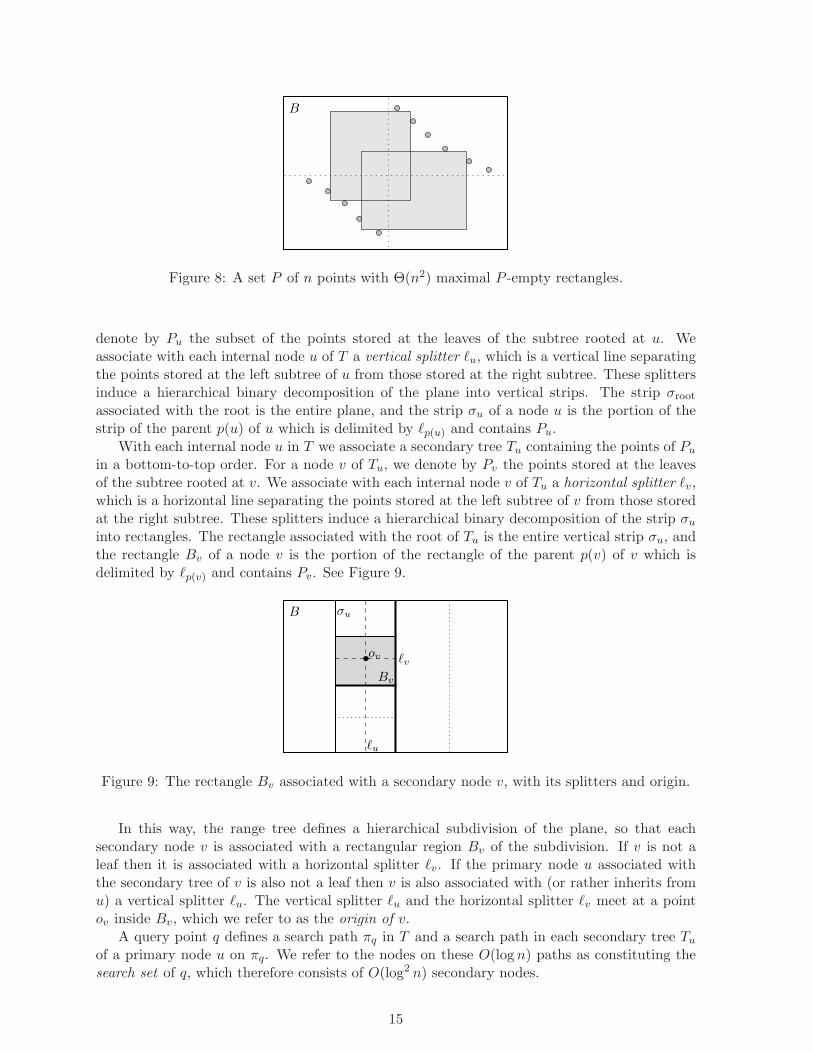
Figure 8: A set P of n points with Θ(n2) maximal P -empty rectangles.

denote by Pu the subset of the points stored at the leaves of the subtree rooted at u. Weassociate with each internal node u of T a vertical splitter ℓu, which is a vertical line separatingthe points stored at the left subtree of u from those stored at the right subtree. These splittersinduce a hierarchical binary decomposition of the plane into vertical strips. The strip σrootassociated with the root is the entire plane, and the strip σu of a node u is the portion of thestrip of the parent p(u) of u which is delimited by ℓp(u) and contains Pu.

With each internal node u in T we associate a secondary tree Tu containing the points of Pu

in a bottom-to-top order. For a node v of Tu, we denote by Pv the points stored at the leavesof the subtree rooted at v. We associate with each internal node v of Tu a horizontal splitter ℓv,which is a horizontal line separating the points stored at the left subtree of v from those storedat the right subtree. These splitters induce a hierarchical binary decomposition of the strip σuinto rectangles. The rectangle associated with the root of Tu is the entire vertical strip σu, andthe rectangle Bv of a node v is the portion of the rectangle of the parent p(v) of v which isdelimited by ℓp(v) and contains Pv. See Figure 9.

B

Bv

ov

ℓu

σu

ℓv

Figure 9: The rectangle Bv associated with a secondary node v, with its splitters and origin.

In this way, the range tree defines a hierarchical subdivision of the plane, so that eachsecondary node v is associated with a rectangular region Bv of the subdivision. If v is not aleaf then it is associated with a horizontal splitter ℓv. If the primary node u associated withthe secondary tree of v is also not a leaf then v is also associated with (or rather inherits fromu) a vertical splitter ℓu. The vertical splitter ℓu and the horizontal splitter ℓv meet at a pointov inside Bv, which we refer to as the origin of v.

A query point q defines a search path πq in T and a search path in each secondary tree Tu

of a primary node u on πq. We refer to the nodes on these O(logn) paths as constituting thesearch set of q, which therefore consists of O(log2 n) secondary nodes.

15

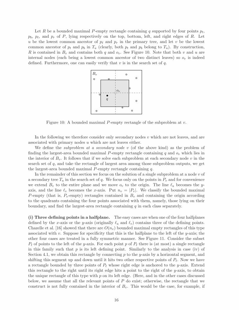
Let R be a bounded maximal P -empty rectangle containing q supported by four points pt,pb, pℓ, and pr of P , lying respectively on the top, bottom, left, and right edges of R. Letu be the lowest common ancestor of pℓ and pr in the primary tree, and let v be the lowestcommon ancestor of pt and pb in Tu (clearly, both pt and pb belong to Tu). By construction,R is contained in Bv and contains both q and ov. See Figure 10. Note that both v and u areinternal nodes (each being a lowest common ancestor of two distinct leaves) so ov is indeeddefined. Furthermore, one can easily verify that v is in the search set of q.

Bv

q

ov

Figure 10: A bounded maximal P -empty rectangle of the subproblem at v.

In the following we therefore consider only secondary nodes v which are not leaves, and areassociated with primary nodes u which are not leaves either.

We define the subproblem at a secondary node v (of the above kind) as the problem offinding the largest-area bounded maximal P -empty rectangle containing q and ov which lies inthe interior of Bv. It follows that if we solve each subproblem at each secondary node v in thesearch set of q, and take the rectangle of largest area among those subproblem outputs, we getthe largest-area bounded maximal P -empty rectangle containing q.

In the remainder of this section we focus on the solution of a single subproblem at a node v ofa secondary tree Tu in the search set of q. We focus only on the points in Pv and for conveniencewe extend Bv to the entire plane and we move ov to the origin. The line ℓu becomes the y-axis, and the line ℓv becomes the x-axis. Put nv = |Pv|. We classify the bounded maximalP -empty (that is, Pv-empty) rectangles contained in Bv and containing the origin accordingto the quadrants containing the four points associated with them, namely, those lying on theirboundary, and find the largest-area rectangle containing q in each class separately.

(i) Three defining points in a halfplane. The easy cases are when one of the four halfplanesdefined by the x-axis or the y-axis (originally ℓu and ℓv) contains three of the defining points.Chazelle et al. [16] showed that there are O(nv) bounded maximal empty rectangles of this typeassociated with v. Suppose for specificity that this is the halfplane to the left of the y-axis; theother four cases are treated in a fully symmetric manner. See Figure 11. Consider the subsetPℓ of points to the left of the y-axis. For each point p of Pℓ there is (at most) a single rectanglein this family such that p is its left defining point. Similarly to the analysis in case (iv) ofSection 4.1, we obtain this rectangle by connecting p to the y-axis by a horizontal segment, andshifting this segment up and down until it hits two other respective points of Pℓ. Now we havea rectangle bounded by three points of Pℓ whose right edge is anchored to the y-axis. Extendthis rectangle to the right until its right edge hits a point to the right of the y-axis, to obtainthe unique rectangle of this type with p on its left edge. (Here, and in the other cases discussedbelow, we assume that all the relevant points of P do exist; otherwise, the rectangle that weconstruct is not fully contained in the interior of Bv. This would be the case, for example, if

16

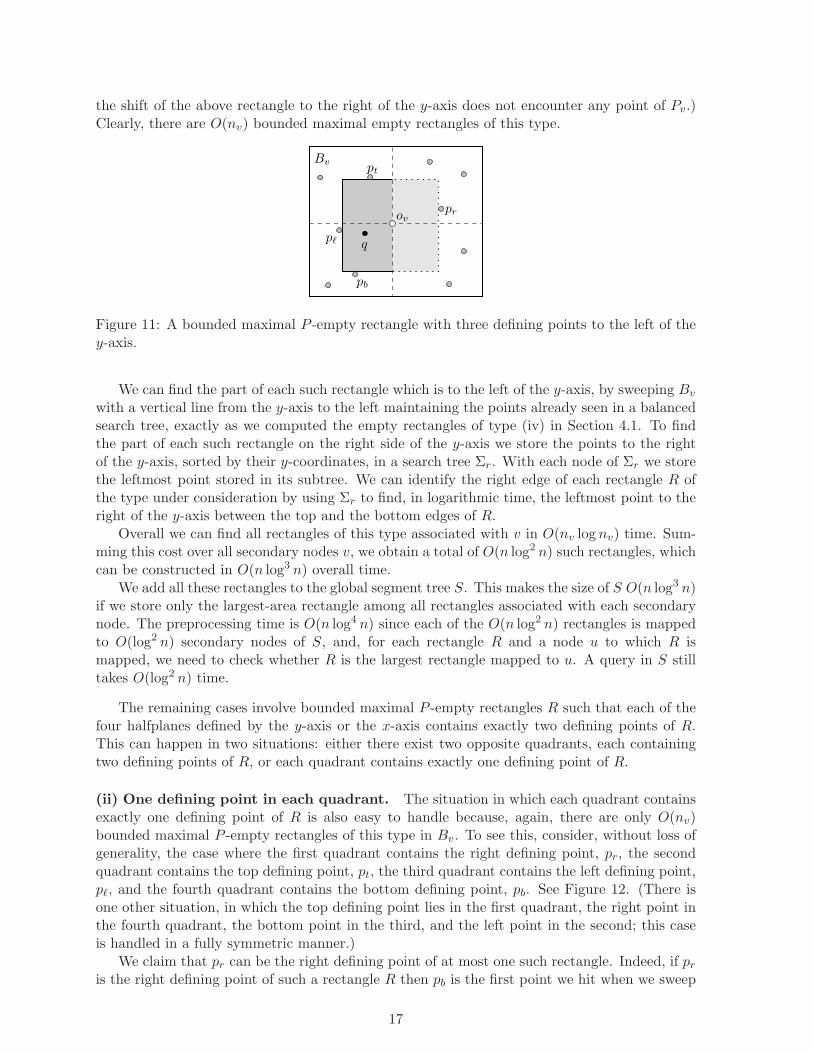
the shift of the above rectangle to the right of the y-axis does not encounter any point of Pv.)Clearly, there are O(nv) bounded maximal empty rectangles of this type.

Bv

qpℓ

ov

pt

pr

pb

Figure 11: A bounded maximal P -empty rectangle with three defining points to the left of they-axis.

We can find the part of each such rectangle which is to the left of the y-axis, by sweeping Bv

with a vertical line from the y-axis to the left maintaining the points already seen in a balancedsearch tree, exactly as we computed the empty rectangles of type (iv) in Section 4.1. To findthe part of each such rectangle on the right side of the y-axis we store the points to the rightof the y-axis, sorted by their y-coordinates, in a search tree Σr. With each node of Σr we storethe leftmost point stored in its subtree. We can identify the right edge of each rectangle R ofthe type under consideration by using Σr to find, in logarithmic time, the leftmost point to theright of the y-axis between the top and the bottom edges of R.

Overall we can find all rectangles of this type associated with v in O(nv lognv) time. Sum-ming this cost over all secondary nodes v, we obtain a total of O(n log2 n) such rectangles, whichcan be constructed in O(n log3 n) overall time.

We add all these rectangles to the global segment tree S. This makes the size of S O(n log3 n)if we store only the largest-area rectangle among all rectangles associated with each secondarynode. The preprocessing time is O(n log4 n) since each of the O(n log2 n) rectangles is mappedto O(log2 n) secondary nodes of S, and, for each rectangle R and a node u to which R ismapped, we need to check whether R is the largest rectangle mapped to u. A query in S stilltakes O(log2 n) time.

The remaining cases involve bounded maximal P -empty rectangles R such that each of thefour halfplanes defined by the y-axis or the x-axis contains exactly two defining points of R.This can happen in two situations: either there exist two opposite quadrants, each containingtwo defining points of R, or each quadrant contains exactly one defining point of R.

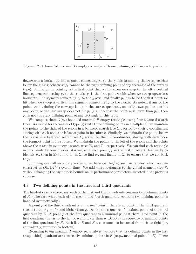
(ii) One defining point in each quadrant. The situation in which each quadrant containsexactly one defining point of R is also easy to handle because, again, there are only O(nv)bounded maximal P -empty rectangles of this type in Bv. To see this, consider, without loss ofgenerality, the case where the first quadrant contains the right defining point, pr, the secondquadrant contains the top defining point, pt, the third quadrant contains the left defining point,pℓ, and the fourth quadrant contains the bottom defining point, pb. See Figure 12. (There isone other situation, in which the top defining point lies in the first quadrant, the right point inthe fourth quadrant, the bottom point in the third, and the left point in the second; this caseis handled in a fully symmetric manner.)

We claim that pr can be the right defining point of at most one such rectangle. Indeed, if pris the right defining point of such a rectangle R then pb is the first point we hit when we sweep

17

Bv

q

prov

pt

pℓ

pb

Figure 12: A bounded maximal P -empty rectangle with one defining point in each quadrant.

downwards a horizontal line segment connecting pr to the y-axis (assuming the sweep reachesbelow the x-axis; otherwise pr cannot be the right defining point of any rectangle of the currenttype). Similarly, the point pℓ is the first point that we hit when we sweep to the left a verticalline segment connecting pb to the x-axis, pt is the first point we hit when we sweep upwards ahorizontal line segment connecting pℓ to the y-axis, and finally pr has to be the first point wehit when we sweep a vertical line segment connecting pt to the x-axis. As noted, if any of thepoints we hit during these sweeps is not in the correct quadrant, one of the sweeps does not hitany point, or the last sweep does not hit pr (e.g., because the point pt is lower than pr), thenpr is not the right defining point of any rectangle of this type.

We compute these O(nv) bounded maximal P -empty rectangles using four balanced searchtrees. As we did for rectangles of type (i) (with three defining points in a halfplane), we maintainthe points to the right of the y-axis in a balanced search tree Σr, sorted by their y coordinates,storing with each node the leftmost point in its subtree. Similarly, we maintain the points belowthe x-axis in a balanced search tree Σb sorted by their x coordinates, storing with each nodethe topmost point in its subtree. We maintain the points to the left of the y-axis and the pointsabove the x-axis in symmetric search trees Σℓ and Σt, respectively. We can find each rectanglein this family by four queries, starting with each point pr in the first quadrant, first in Σb toidentify pb, then in Σℓ to find pℓ, in Σt to find pt, and finally in Σr to ensure that we get backto pr.

Summing over all secondary nodes v, we have O(n log2 n) such rectangles, which we canconstruct in O(n log3 n) overall time. We add these rectangles to the global segment tree S,without changing the asymptotic bounds on its performance parameters, as noted in the previoussubcase.

4.3 Two defining points in the first and third quadrants

The hardest case is where, say, each of the first and third quadrants contains two defining pointsof R. (The case where each of the second and fourth quadrants contains two defining points ishandled symmetrically.)

A point p of the third quadrant is a maximal point if there is no point in the third quadrantthat is to the right of p and higher than p. Denote the sequence of maximal points of the thirdquadrant by E. A point p of the first quadrant is a minimal point if there is no point in thefirst quadrant that is to the left of p and lower than p. Denote the sequence of minimal pointsof the first quadrant by F . Both lists E and F are assumed to be sorted from left to right (or,equivalently, from top to bottom).

Returning to our maximal P -empty rectangle R, we note that its defining points in the first(resp., third) quadrant are consecutive minimal points in F (resp., maximal points in E). There

18

are O(nv) such pairs in both lists.Consider a consecutive pair (a, b) in E (with a to the left and above b). Let M1 be the unique

P -empty rectangle whose right edge is anchored at the y-axis, its left edge passes through a,its bottom edge passes through b, and its top edge passes through some point c (in the secondquadrant); it is possible that c does not exist, in which case some minor modifications (actually,simplifications) need to be applied to the forthcoming analysis, which we do not spell out.

Similarly, let M2 be the unique P -empty rectangle whose top edge is anchored at the x-axis,its left edge passes through a, its bottom edge passes through b, and its right edge passes throughsome point d (in the fourth quadrant; again, we ignore the case where d does not exist). SeeFigure 13. Our maximal P -empty rectangle cannot extend higher than c, nor can it extend tothe right of d. Hence its two other defining points must be a pair (w, z) of consecutive elementsof F , both lying to the left of d and below c. The minimal points which satisfy these constraintsform a contiguous subsequence of F .

c

d

ba

Figure 13: The structure of maximal empty rectangles with two defining points in each ofthe first and third quadrants. For each consecutive pair ρ = (a, b) of maximal points in thethird quadrant, there is an “interval” Iρ of minimal points in the first quadrant such that anyconsecutive pair of points in Iρ define with ρ a maximal empty rectangle. The point c in thesecond quadrant and the point d in the fourth quadrant define Iρ.

That is, for each consecutive pair ρ = (a, b) of points of E we have a contiguous “interval”Iρ ⊆ F , so that any consecutive pair π = (w, z) of points in Iρ defines with ρ a maximal P -empty rectangle which contains the origin, and these are the only pairs which can define with ρsuch a rectangle. (Note that we can ignore the “extreme” rectangles defined by a, b, c, and thehighest point of Iρ, or by a, b, d, and the lowest point of Iρ, since these rectangles have threeof their defining points in a common halfplane defined by the x-axis or by the y-axis, and havetherefore already been treated.)

To answer queries with respect to these rectangles, we process the data as follows. Wecompute the chain E of maximal points in the third quadrant and the chain F of minimalpoints in the first quadrant, ordered as above. This is done in O(nv lognv) time in the sameway as we computed the chain of maximal points of P in Section 4.1. For each pair ρ = (a, b)of consecutive points in E we compute the corresponding delimiting points c (in the secondquadrant) and d (in the fourth quadrant). Formally, c is the lowest point in the second quadrant

19

which lies to the right of a, and d is the leftmost point in the fourth quadrant which lies aboveb. We then use c and d to “carve out” the interval Iρ of F , consisting of those points thatlie below c and to the left of d. We can find c by a binary search in the chain of y-minimaland x-maximal points in the second quadrant, and find d by a binary search in the chain ofx-minimal and y-maximal points in the fourth quadrant. These chains can be computed in thesame way as in the construction of E and F . Once we have the chains we can find, for eachconsecutive pair ρ = (a, b) in E, the corresponding entities c, d, and Iρ, in O(lognv) time.

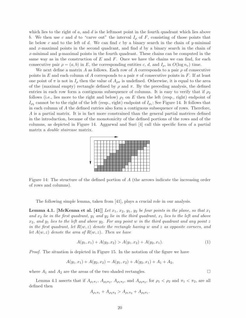
We next define a matrix A as follows. Each row of A corresponds to a pair ρ of consecutivepoints in E and each column of A corresponds to a pair π of consecutive points in F . If at leastone point of π is not in Iρ then the value of Aρπ is undefined. Otherwise, it is equal to the areaof the (maximal empty) rectangle defined by ρ and π. By the preceding analysis, the definedentries in each row form a contiguous subsequence of columns. It is easy to verify that if ρ2follows (i.e., lies more to the right and below) ρ1 on E then the left (resp., right) endpoint ofIρ2 cannot be to the right of the left (resp., right) endpoint of Iρ1 ; See Figure 14. It follows thatin each column of A the defined entries also form a contiguous subsequence of rows. Therefore,A is a partial matrix. It is in fact more constrained than the general partial matrices definedin the introduction, because of the monotonicity of the defined portions of the rows and of thecolumns, as depicted in Figure 14. Aggarwal and Suri [4] call this specific form of a partialmatrix a double staircase matrix.

Figure 14: The structure of the defined portion of A (the arrows indicate the increasing orderof rows and columns).

The following simple lemma, taken from [41], plays a crucial role in our analysis.

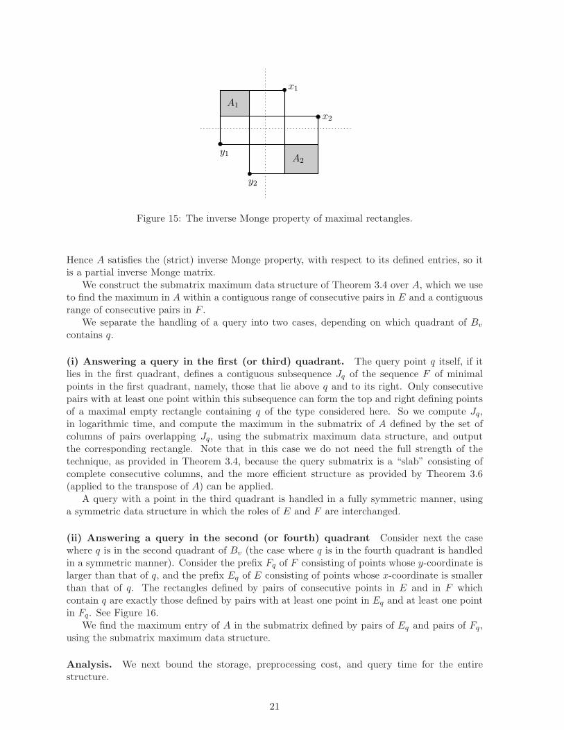
Lemma 4.1. [McKenna et al. [41]] Let x1, x2, y1, y2 be four points in the plane, so that x1and x2 lie in the first quadrant, y1 and y2 lie in the third quadrant, x1 lies to the left and abovex2, and y1 lies to the left and above y2. For any point w in the third quadrant and any point zin the first quadrant, let R(w, z) denote the rectangle having w and z as opposite corners, andlet A(w, z) denote the area of R(w, z). Then we have

A(y1, x1) +A(y2, x2) > A(y1, x2) +A(y2, x1). (1)

Proof. The situation is depicted in Figure 15. In the notation of the figure we have

A(y1, x1) +A(y2, x2) = A(y1, x2) +A(y2, x1) +A1 +A2,

where A1 and A2 are the areas of the two shaded rectangles.

Lemma 4.1 asserts that if Aρ1π1, Aρ2π2

, Aρ1π2, and Aρ2π2

, for ρ1 < ρ2 and π1 < π2, are alldefined then

Aρ1π1+Aρ2π2

> Aρ1π2+Aρ2π1

.

20

x1

x2

y1

y2

A1

A2

Figure 15: The inverse Monge property of maximal rectangles.

Hence A satisfies the (strict) inverse Monge property, with respect to its defined entries, so itis a partial inverse Monge matrix.

We construct the submatrix maximum data structure of Theorem 3.4 over A, which we useto find the maximum in A within a contiguous range of consecutive pairs in E and a contiguousrange of consecutive pairs in F .

We separate the handling of a query into two cases, depending on which quadrant of Bv

contains q.

(i) Answering a query in the first (or third) quadrant. The query point q itself, if itlies in the first quadrant, defines a contiguous subsequence Jq of the sequence F of minimalpoints in the first quadrant, namely, those that lie above q and to its right. Only consecutivepairs with at least one point within this subsequence can form the top and right defining pointsof a maximal empty rectangle containing q of the type considered here. So we compute Jq,in logarithmic time, and compute the maximum in the submatrix of A defined by the set ofcolumns of pairs overlapping Jq, using the submatrix maximum data structure, and outputthe corresponding rectangle. Note that in this case we do not need the full strength of thetechnique, as provided in Theorem 3.4, because the query submatrix is a “slab” consisting ofcomplete consecutive columns, and the more efficient structure as provided by Theorem 3.6(applied to the transpose of A) can be applied.

A query with a point in the third quadrant is handled in a fully symmetric manner, usinga symmetric data structure in which the roles of E and F are interchanged.

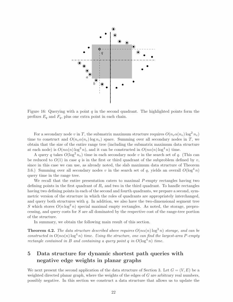
(ii) Answering a query in the second (or fourth) quadrant Consider next the casewhere q is in the second quadrant of Bv (the case where q is in the fourth quadrant is handledin a symmetric manner). Consider the prefix Fq of F consisting of points whose y-coordinate islarger than that of q, and the prefix Eq of E consisting of points whose x-coordinate is smallerthan that of q. The rectangles defined by pairs of consecutive points in E and in F whichcontain q are exactly those defined by pairs with at least one point in Eq and at least one pointin Fq. See Figure 16.

We find the maximum entry of A in the submatrix defined by pairs of Eq and pairs of Fq,using the submatrix maximum data structure.

Analysis. We next bound the storage, preprocessing cost, and query time for the entirestructure.

21

q

a

b

Figure 16: Querying with a point q in the second quadrant. The highlighted points form theprefixes Eq and Fq, plus one extra point in each chain.

For a secondary node v in T , the submatrix maximum structure requires O(nvα(nv) log2 nv)

time to construct and O(nvα(nv) log nv) space. Summing over all secondary nodes in T , weobtain that the size of the entire range tree (including the submatrix maximum data structureat each node) is O(nα(n) log3 n), and it can be constructed in O(nα(n) log4 n) time.

A query q takes O(log2 nv) time in each secondary node v in the search set of q. (This canbe reduced to O(1) in case q is in the first or third quadrant of the subproblem defined by v,since in this case we can use, as already noted, the slab maximum data structure of Theorem3.6.) Summing over all secondary nodes v in the search set of q, yields an overall O(log4 n)query time in the range tree.

We recall that the entire presentation caters to maximal P -empty rectangles having twodefining points in the first quadrant of Bv and two in the third quadrant. To handle rectangleshaving two defining points in each of the second and fourth quadrants, we prepare a second, sym-metric version of the structure in which the roles of quadrants are appropriately interchanged,and query both structures with q. In addition, we also have the two-dimensional segment treeS which stores O(n log2 n) special maximal empty rectangles. As noted, the storage, prepro-cessing, and query costs for S are all dominated by the respective cost of the range-tree portionof the structure.

In summary, we obtain the following main result of this section.

Theorem 4.2. The data structure described above requires O(nα(n) log3 n) storage, and can beconstructed in O(nα(n) log4 n) time. Using the structure, one can find the largest-area P -emptyrectangle contained in B and containing a query point q in O(log4 n) time.

5 Data structure for dynamic shortest path queries withnegative edge weights in planar graphs

We next present the second application of the data structure of Section 3. Let G = (V,E) be aweighted directed planar graph, where the weights of the edges of G are arbitrary real numbers,possibly negative. In this section we construct a data structure that allows us to update the

22

weight of an edge, and to query for the distance between two arbitrary nodes u, v, namely,the smallest total weight of a path connecting u to v in G. The data structure requires linearstorage and near-linear preprocessing, and answers a query or an update in O(n2/3 log5/3(n))time.

Our data structure is based on the data structure of Klein [38], which only supports non-negative edge weights. We overcome this restriction by using reduced costs [33] which transformthe problem into one with non-negative weights. Klein’s data structure uses a data structure ofFakcharoenphol and Rao [24] that implements Dijkstra’s algorithm efficiently. When using re-duced costs, certain range minima data structures used in the data structure of Fakcharoenpholand Rao must be reconstructed after each weight update. We replace these components of thedata structure with our row-interval minima data structure from Lemma 3.1 which has a fasterconstruction time. We note that this idea, of using our new row-interval minima data structurein the data structure of Fakcharoenphol and Rao, has recently been used in the context ofcomputing maximum flow in planar graphs [10]. The application to dynamic data structuresfor distance computations in planar graphs is new.

In Section 5.1 we describe Klein’s data structure for distance queries on a dynamic planargraph with non-negative edge weights. In Section 5.2 we describe Fakcharoenphol and Rao’simplementation of Dijkstra’s algorithm [24] on the so called Dense Distance Graph (DDG) whichis defined below. The basic data structure underlying their implementation, which we refer toas the Monge heap, is described in Section 5.3. With all this background handy, we describe inSection 5.4 how to modify Klein’s data structure to allow negative edge weights. In Section 5.5we show how to augment our data structure so that it can report the shortest path itself.

We make the following assumptions about G.

• We assume that G is simple, which can be ensured by removing self-loops and leavingonly the shortest among each set of parallel edges.

• We assume that G is embedded in the plane (in the standard terminology, G is a planegraph). A plane embedding of G can be found in linear time (see, e.g., [31]).

• We assume that there are no cycles whose total weight is negative; if such a cycle iscreated due to a weight update, then our data structure will detect it (and abort theentire dynamic maintenance of G).

We denote the number of nodes by n. Since G is planar and simple, we have |E| = O(n).By a piece of G we refer to an edge-induced subgraph of G.11 Fix some parameter r < n. An

r-division, depicted in Figure 17, is a partition of E into O(n/r) pieces such that the followingadditional properties hold.12 (i) Each piece contains O(r) nodes. We call a node which lies inmore than one piece a boundary node. (ii) Each piece has O(

√r) boundary nodes. Fredrickson

[26] showed how to compute such an r-division in O(n log r + n√rlog n) time, based on the

Lipton-Tarjan planar separator theorem [40].13

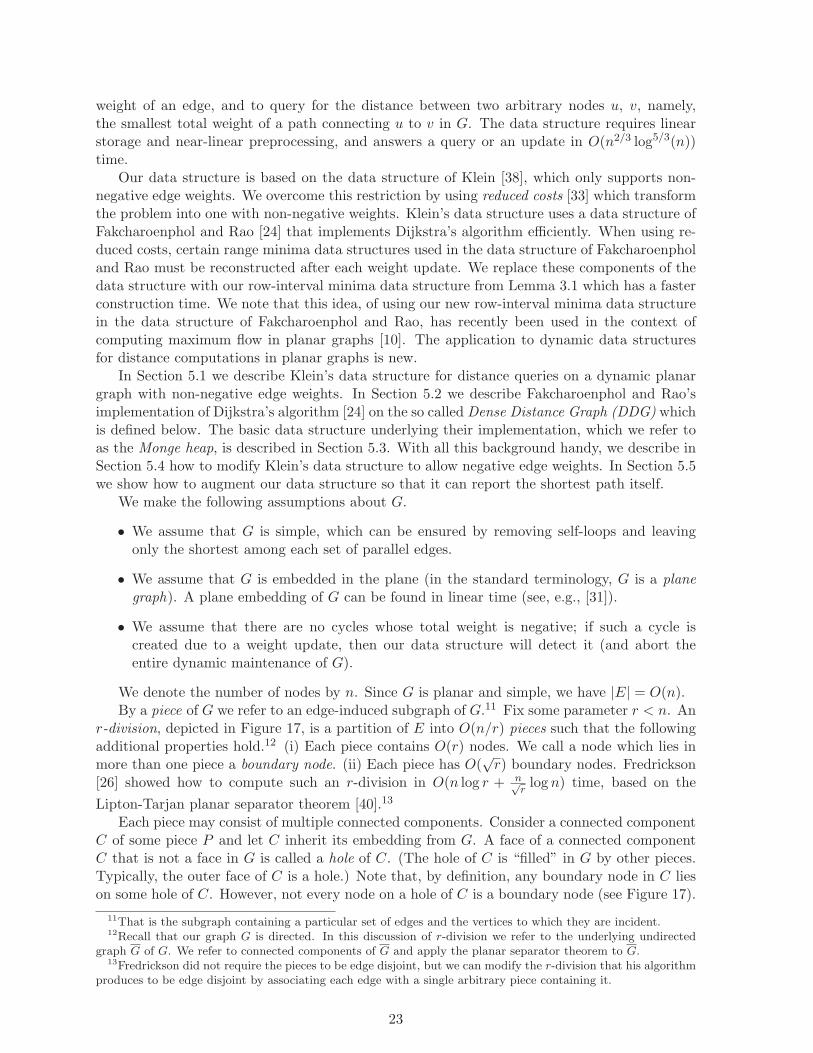
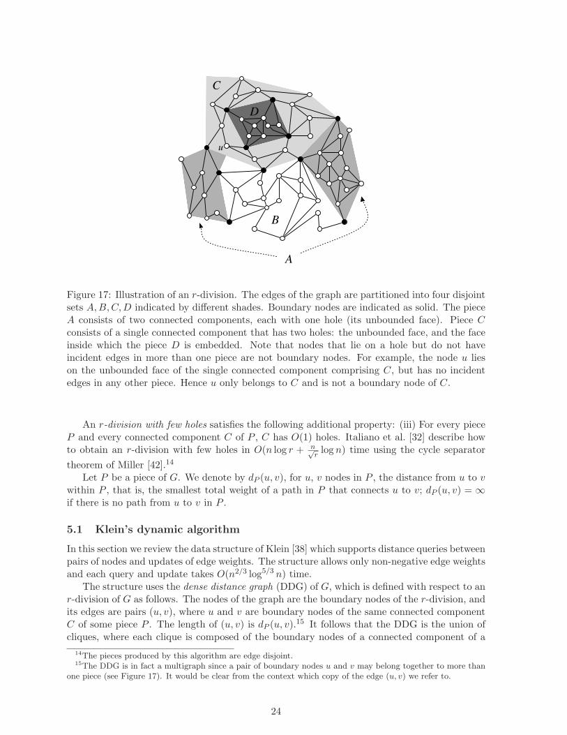
Each piece may consist of multiple connected components. Consider a connected componentC of some piece P and let C inherit its embedding from G. A face of a connected componentC that is not a face in G is called a hole of C. (The hole of C is “filled” in G by other pieces.Typically, the outer face of C is a hole.) Note that, by definition, any boundary node in C lieson some hole of C. However, not every node on a hole of C is a boundary node (see Figure 17).

11That is the subgraph containing a particular set of edges and the vertices to which they are incident.12Recall that our graph G is directed. In this discussion of r-division we refer to the underlying undirected

graph G of G. We refer to connected components of G and apply the planar separator theorem to G.13Fredrickson did not require the pieces to be edge disjoint, but we can modify the r-division that his algorithm

produces to be edge disjoint by associating each edge with a single arbitrary piece containing it.

23

A

B

C

D

u

Figure 17: Illustration of an r-division. The edges of the graph are partitioned into four disjointsets A,B,C,D indicated by different shades. Boundary nodes are indicated as solid. The pieceA consists of two connected components, each with one hole (its unbounded face). Piece Cconsists of a single connected component that has two holes: the unbounded face, and the faceinside which the piece D is embedded. Note that nodes that lie on a hole but do not haveincident edges in more than one piece are not boundary nodes. For example, the node u lieson the unbounded face of the single connected component comprising C, but has no incidentedges in any other piece. Hence u only belongs to C and is not a boundary node of C.

An r-division with few holes satisfies the following additional property: (iii) For every pieceP and every connected component C of P , C has O(1) holes. Italiano et al. [32] describe howto obtain an r-division with few holes in O(n log r + n√

rlogn) time using the cycle separator

theorem of Miller [42].14

Let P be a piece of G. We denote by dP (u, v), for u, v nodes in P , the distance from u to vwithin P , that is, the smallest total weight of a path in P that connects u to v; dP (u, v) = ∞if there is no path from u to v in P .

5.1 Klein’s dynamic algorithm

In this section we review the data structure of Klein [38] which supports distance queries betweenpairs of nodes and updates of edge weights. The structure allows only non-negative edge weightsand each query and update takes O(n2/3 log5/3 n) time.

The structure uses the dense distance graph (DDG) of G, which is defined with respect to anr-division of G as follows. The nodes of the graph are the boundary nodes of the r-division, andits edges are pairs (u, v), where u and v are boundary nodes of the same connected componentC of some piece P . The length of (u, v) is dP (u, v).

15 It follows that the DDG is the union ofcliques, where each clique is composed of the boundary nodes of a connected component of a

14The pieces produced by this algorithm are edge disjoint.15The DDG is in fact a multigraph since a pair of boundary nodes u and v may belong together to more than

one piece (see Figure 17). It would be clear from the context which copy of the edge (u, v) we refer to.

24

single piece.Fakcharoenphol and Rao [24] gave an implementation of Dijkstra’s algorithm that runs on

the DDG of G, for any fixed source vertex, in O((n/√r) log n log r) time and uses O(n) space.

We describe the relevant details of this implementation in Section 5.2. This implementationrequires, for each connected component of a piece, a data structure which we call, for short, aMonge heap (Fakcharoenphol and Rao call it an on-line Monge searching data structure). Theconstruction of the Monge heaps of the connected components of a single piece takes O(r log r)time, and since there are O(n/r) pieces, the construction time of the entire representation of theDDG is O(n log r) [38]. It follows that the total construction time of this static data structure(i.e., computing the r-division, and the Monge heaps, each representing the contribution of aconnected component of some piece to the DDG. All these computations are done only once.)takes O(n logn) time for our choice of r (which would be n2/3 log2/3 n).

The algorithm for answering a distance query from a node s in a piece Ps to a node t in apiece Pt consists of three steps:16

1. In the first step we find the distance inside Ps from s to every node of Ps, in O(r log r)time, using Dijkstra’s algorithm. (This distance is ∞ for nodes of Ps outside the connectedcomponent containing s.) In particular we get the distance from s to every boundary nodeof Ps.

17 If Ps = Pt, that is, s and t are in the same piece, then this step computes inparticular dPs(s, t) (which of course does not have to be equal to the shortest distancebetween s and t). Note that we can skip this step if s is a boundary node of Ps.

2. In the second step we run an implementation of Dijkstra’s algorithm, due to Fakcharoen-phol and Rao [24], on the DDG, initializing the distance labels of the boundary nodesof Ps with their distances dPs(s, ·) from s, as computed in the first step, and initializingthe labels for all other nodes to ∞.18 By doing this we simulate a single source shortestpath computation in the DDG from an artificial source connected to each boundary nodev of Ps by an edge whose weight is the distance from s to v in Ps. This implementation,described in Section 5.2, runs in O((n/

√r) log n log r) time and uses O(n) space.

3. In the third step, we compute the distance from the boundary nodes of Pt to t inside Pt

where the initial distance labels of the boundary nodes of Pt are their distances from s,as computed in the previous step. By doing this we simulate a single source shortest pathcomputation inside Pt from an artificial source connected to each boundary node v of Pt byan edge whose weight is the distance from s to v as computed in Step (2). We implementthis step by running Dijkstra’s algorithm inside Pt with the appropriate initialization,which takes O(r log r) time. Note that we can skip this step if t is a boundary node of Pt.

Upon termination of the third step we can easily compute the weight ℓ of the shortest pathfrom s to t among those containing a boundary node. If s and t are in different pieces the distancebetween them is ℓ, and if they are in the same piece P then the distance is mindP (s, t), ℓ.

The correctness of the query algorithm is a consequence of the following property of shortestpaths.

Lemma 5.1. Assume that s and t belong to pieces, Ps and Pt, respectively. Let s = v0, v1, . . . , vk =t be any shortest path from s to t. Then either Ps = Pt and s = v0, v1, . . . , vk = t is a path in

16If s or t are boundary nodes, the choice of Ps or Pt, respectively, will not matter, as we indicate below.17Klein [38] uses a multiple-source shortest-path data structure for this purpose, and finds the distances from

s to all boundary nodes of Ps faster, in O(√r log r) time; however this does not affect the overall asymptotic cost

of the algorithm.18If s is a boundary node then we simply initialize its label to 0 and all other labels to ∞.

25

Ps, or there exists an increasing sequence of indices 0 ≤ i0 < i1 < · · · < iℓ ≤ k such that, forany 0 ≤ j ≤ ℓ, vij is a boundary node, and the following holds.

1. v0, v1, . . . vi0 is a shortest path in Ps from s to vi0.

2. for any 0 ≤ j < ℓ, vij , vij+1, . . . , vij+1is a shortest path from vij to vij+1

in some piece P .(In particular vij and vij+1

are boundary nodes of the same piece P .)

3. viℓ , viℓ+1, . . . vk is a shortest path in Pt from viℓ to t.

Proof. Follows immediately from the definition of boundary nodes and from the fact that, inthe absence of negative-weight cycles, for any 0 ≤ i ≤ j ≤ k, vi, vi+1, . . . , vj is a shortest pathfrom vi to vj .

To update the weight of an edge e, we reconstruct from scratch the Monge heap associatedwith the (unique) connected component C of the piece P to which e belongs.

To conclude, a distance query to Klein’s data structure takes O(r log r+ (n/√r) log n log r)

time, and the time for a weight update of an edge is O(r log r). By setting r = n2/3 log2/3 n, weget that the time for each update and query is O(n2/3 log5/3 n).

The query algorithm described here only works with non-negative edge weights because ituses an implementation of Dijkstra’s algorithm to compute shortest paths. We show how toextend the algorithm for negative edge weights in Section 5.4.

5.2 Fast Dijkstra on the dense distance graph

We describe here the fast implementation of Dijkstra’s algorithm on the dense distance graph(DDG) due to Fakcharoenphol and Rao [24, Section 3.2.2]. We run this procedure in the contextof answering a distance query from some node s to another node t. We have initial distancelabels for the nodes of the DDG as set in Step 2 of the query, described in the precedingsubsection, and we want to run Dijkstra’s algorithm on the DDG starting with these initiallabels. Recall that Dijkstra’s algorithm works as follows. It maintains a heap of the nodes, eachwith its distance label as the key. As long as there are nodes in the heap with a finite distancelabel, we extract the node u with the minimum label and relax all the edges emanating from u.That is, for each edge (u, v) we set δ(v) := minδ(v), δ(u)+w(u, v), where δ(v) is the distancelabel of v and w(u, v) is the weight of the edge (u, v). Upon termination, the distance label ofeach boundary node v is equal to the distance from s to v in G.19

By construction, the DDG has O(√r(n/r)) = O(n/

√r) nodes and O((

√r)2(n/r)) = O(n)

edges. A naive implementation of Dijkstra’s algorithm therefore takes Ω(n) time, which is tooslow for our purpose. The technique of Fakcharoenphol and Rao overcomes this difficulty byexploiting the Monge-like property of the edges of the DDG to avoid relaxing each edge explicitly(see below for details).

We use a separate Monge heap for each connected component of each piece. To simplifyour presentation we will assume in the following description that each piece P is connected andthereby there is only one Monge heap associated with P . If P has multiple components wesimply apply the exact same construction to each connected component separately.

The Monge heap data structure of a piece P , denoted as MHP , maintains a distance labelδP (v) for each boundary node v of P . At any time during the run of Dijkstra’s algorithm, δP (v)is the length of the shortest path to v whose last edge is in P , among all such paths encounteredso far. Note that, by definition, each boundary node v belongs to at least two distinct pieces,

19Dijkstra’s algorithm also maintains a predecessor π(v) for each vertex v to find the shortest path tree itself.It updates π(v) to be u when a relaxation of an edge (u, v) changes δ(v).

26

and its labels within each piece may differ. MHP supports the following operations. (To simplifythe notation we usually do not write P as an explicit parameter of these functions. Each Mongeheap has such a set of functions and it knows the piece P it is associated with.)

• FindMinInPiece(): Return a boundary node v in MHP with minimum δP (v).

• ExtractMinInPiece(): Extract a boundary node v from MHP with minimum δP (v).20

• ScanInPiece(v, d): Implicitly relax all the edges emanating from v in P , given that thetrue distance from s to v in G is d.21 Recall that in the DDG all boundary nodes of P forma (bi-directional) clique. This operation implicitly sets δP (u) := minδP (u), d+ dP (v, u)for every boundary node u of P which is still in MHP .

We also maintain a standard (global) heap H similar to the heap of the standard implemen-tation of Dijkstra’s algorithm. We denote by δ(v) the key of a node v in H. We store in H twokinds of nodes.

1. Nodes v with minimum distance labels in the Monge heaps. If v is the minimum of aMonge heap MHP then we say that v is the representative of MHP in H. Each node vis stored with a reference to MHP , the Monge heap which it represents, and the key δ(v)of such a node v in H is its distance label in MHP . (The same node v may appear in Hmultiple times with different keys as a representative of different Monge heaps.)

2. Boundary nodes of the piece containing s with initial finite distance label. The key δ(v)of such a node v in H is its initial distance label.

For every boundary node v we keep a bit indicating whether v was already visited or not.In contrast to standard implementations of Dijkstra’s algorithm, we need to keep a record ofwhether a node v was already visited, since multiple copies of v may be stored in H. Thishappens since v has copies in more than one piece, and each such copy might be the repre-sentative of its piece in H. (Node v can also be in H if it is a boundary node of the piece ofs with an initial finite distance label.) Moreover, due to the specific way in which the Mongeheaps are implemented, as explained in the next subsection, there are O(log r) copies of eachnode in a single Monge heap; consequently a node v may become the minimum of this heapO(log r) times (and inserted as a representative into H). However, if we restrict the sequenceof node extractions from H to the first extraction of each node then this subsequence of nodeextractions is identical to the sequence of node extractions performed by a traditional imple-mentation of Dijkstra’s algorithm. That is when a node v is first extracted from H, v is reallythe node with the minimum distance label picked by a traditional implementation of Dijkstra’salgorithm. The other extractions are fictitious artifacts of the implementation and they whenthey occur.

Initially, for every boundary node v of the piece P containing s with initial distance labeldP (s, v) we set δ(v) := dP (s, v), and insert v with key δ(v) into H.

In each iteration we extract from H the minimum element. Let v be the node correspondingto the extracted element. If v is the minimum element of a Monge heap MHP of a piece P thenwe perform ExtractMinInPiece() in P to delete this copy of v from MHP . We find the newminimum in P by executing FindMinInPiece() of MHP , and insert the new minimum into H.

If v is already marked as visited we do nothing else and continue to the next iteration.Otherwise, we mark v as visited and set d(s, v) = δ(v); that is, the key of v in H is the distance

20ExtractMinInPiece and FindMinInPiece return the same node in case of ties.21Amajor property of Dijkstra’s algorithm, also used in this implementation, is that it performs relax operations

from a node v only after finding the true distance of v from s.

27

of v from s. For every piece P ′ containing v we perform ScanInPiece(v, d(s, v)) in MHP ′ ,followed by FindMinInPiece() in MHP ′ . We update the element contributed to H by MHP ′

if it has changed or insert the minimum element of MHP ′ to H if this is our first operation onMHP ′ .

As we show in the next subsection, FindMinInPiece() takes O(1) worst-case time, Ex-tractMinInPiece() takes O(log r) worst-case time, and ScanInPiece() takes O(log2 r) amor-tized time. Since the cost of a call to FindMinInPiece() is no larger than the cost of a call toExtractMinInPiece() or to ScanInPiece(), and each time we call FindMinInPiece() wealso call either ExtractMinInPiece() or ScanInPiece(), we can charge the total cost of thecalls to FindMinInPiece() to the overall cost of the calls to ExtractMinInPiece() and toScanInPiece().

A boundary node v of a piece P is returned O(log r) times by calls to ExtractMinIn-Piece() in P (see the next subsection for details), and we call ScanInPiece(v, d) once. Sincethere are O(n/r) pieces, each with O(

√r) boundary nodes, the total time spent on calls to these

procedures is O((n/√r) log2 r). However, the running time is dominated by the time spent on

extracting the minimum elements from the global heap H.Consider the size of the heap H at some specific time during the run of the algorithm. Each

piece can contribute each of its boundary nodes to the global heap H at most once as therepresentative of the connected component containing it. Since there are O(n/r) pieces, eachwith O(

√r) boundary nodes the number of elements in H at any particular time is O(n/

√r). It

follows that the time to find the minimum element in H is O(log(n/√r)) = O(log n). Since the

total number of boundary nodes is O(n/√r), and since each boundary node may be inserted

into H O(log r) times (see the next subsection for details), the number of times we extractminimum elements from H is O((n/

√r) log r). Hence the total running time of this variant of

Dijkstra’s algorithm on the dense distance graph is O((n/√r) log n log r).

5.3 Monge heaps

In this subsection we describe the implementation of the Monge heap data structure MHP ofa piece P , given by Fakcharoenphol and Rao in [24, Section 4]. Recall that we simplify thepresentation by assuming that each piece is connected. Otherwise, we construct a separateMonge heap, as described here, for every connected component of a piece. We start with asimple case in which (the connected component of) P has only one hole.

The first component of the Monge heap is a matrix M representing all edges contributed byP to the DDG. The rows (resp., columns), in the increasing order of their indices, correspond tothe boundary nodes of P in clockwise (resp., counterclockwise) order around the boundary of thehole. The entry Muv contains dP (u, v). In addition, for every boundary node u, Fakcharoenpholand Rao construct a range minima data structure over the row of u in M , to query for a nodev minimizing dP (u, v) within a contiguous subsequence of boundary nodes along the boundaryof the hole. Fakcharoenphol and Rao used a simple search tree-based range minima structurefor this purpose.

Because of the cyclic nature of the order of the nodes along the hole boundary, the ma-trix M does not necessarily have the Monge property. This however can be fixed, as done byFakcharoenphol and Rao, by splitting M into disjoint submatrices, such that each submatrixdoes have the Monge property. Specifically, the boundary nodes of P are split into two con-tiguous sequences A and B of (roughly) equal length. Then the submatrix of M whose rowscorrespond to the nodes of A and whose columns correspond to the nodes of B is a Mongematrix. (This is argued in much the same way as in Monge’s original observation, mentionedin the introduction.) Similarly, the submatrix of M whose rows correspond to the nodes of

28

B and whose columns correspond to the nodes of A is also a Monge matrix. We recursivelysplit the remaining submatrices A × A and B × B in the same way, until we get to sequencesof length 1. See Figure 18 for an illustration. Together, all the submatrices defined by thisrecursive partitioning of M are pairwise disjoint and cover M . Note that each boundary nodeis contained in O(log r) submatrices.

B A

A

B

(a) Submatrices resulting from thefirst three levels of the recursive de-composition are shown. The shadedblocks require further decomposi-tion.

v

A B

(b) Illustration of the correspond-ing partitions of boundary nodes.All bipartitions in which a particularnode v appears are indicated.

Figure 18: Illustration of the decomposition of M into Monge Submatrices.

The initialization of the Monge heap consists of computing (explicitly, all entries of) M ,splitting it into submatrices, and constructing the range minima data structures. Since allboundary nodes lie on a single hole, computing the entries of M (i.e., distances between allpairs of boundary nodes) takes O(r log r) time and O(r) space using Klein’s multiple-sourceshortest-path algorithm [38] (see also [14]). It can be easily verified that all the other tasks canbe performed within the same time and space bounds. This entire process is done once, duringpreprocessing, before handling any query or update.

During a distance computation we maintain, for each submatrix M ′, a bipartite Monge sub-heap (Fakcharoenphol and Rao call it a bipartite on-line Monge searching data structure), whichsupports the Monge heap operations restricted to the bipartite subgraph that M ′ represents,using the fact that the submatrix has the Monge property.

The bipartite Monge subheap. The bipartite Monge subheap H ′ of a Monge submatrixM ′ with a set of rows A and a set of columns B maintains a distance label δ′(u) for every nodeu ∈ A. Initially δ′(u) = ∞ for every u ∈ A. The distance label of a node v ∈ B is defined tobe δ′(v) = minu∈Aδ′(u) +M ′

uv (recall that M ′uv = dP (u, v)) and is not stored explicitly. For

every node v ∈ B we maintain a bit indicating whether v has already been extracted from H ′ ornot. Initially all nodes of B are in H ′. A node v is extracted from H ′ when it has the smallestdistance label among all nodes in the global heap H and therefore also in the Monge heap MHP

containing H ′. The monotonicity of the smallest label in Dijkstra’s algorithm implies that afterv is extracted from H ′ a subsequent decrease in δ′(u) for a node u ∈ A cannot cause δ′(v) todecrease: the value of δ′(u) (which will always be lower bounded by d(s, v)) cannot be smallerthan the value of δ′(v) when it was extracted from H ′.

The bipartite Monge subheap structure supports the following operations (H ′ is implicit inthe following notation):

29

• FindMin(): Return a node v ∈ B with minimum distance label δ′(v) among those thathave not yet been extracted.

• ExtractMin(): Extract a node v ∈ B with minimum distance label δ′(v) among thosethat have not yet been extracted.22

• Scan(u, d): Set δ′(u) = d for u ∈ A, and (implicitly) relax all the edges from u to thenodes of B.

We say that u ∈ A is the parent of v ∈ B (and v is the child of u) if δ′(u) is finite andδ′(v) = δ′(u) + M ′

uv; see below for handling ties. As the execution of Dijkstra’s algorithmprogresses, the distance labels δ′(u) of nodes u ∈ A may change and thereby the parents ofnodes v ∈ B may change. Assuming that the parent of every member of v ∈ B is uniquelydefined (at some fixed time), the Monge property of M ′ implies the following two properties:

1. The set of nodes of B for which a specific node u ∈ A is the parent are consecutive in B.

2. If node u′ follows u in A, then the set of nodes of which u′ is the parent follows in B theset of nodes of which u is the parent.

Furthermore, in case of ties, i.e. when there are two different nodes u1, u2 ∈ A such thatδ′(v) = δ′(u1) +M ′

u1v = δ′(u2) +M ′u2v, the Monge property of M ′ implies that we can always

break the tie and pick a parent for v such that Properties (1) and (2) above continue to besatisfied. Our algorithm will indeed (implicitly) maintain parents in this manner such thatProperties (1) and (2) are satisfied. Note that nodes in B with infinite distance labels will alsohave parents in A. For such a node v any node u ∈ A satisfies that δ′(v) = δ′(u) +M ′

uv and wecan pick any node to be a parent of v as long as we maintain Properties (1) and (2).

We maintain a binary search tree T of triplets of the form (a, b1, b2) where a ∈ A, b1, b2 ∈ B,and the set of nodes of B between b1 and b2 (inclusive) is a maximal interval of nodes of B thatare currently in H ′ and whose parent is a. See Figure 19. Note that the same node a ∈ A mayappear in more than one triplet of T because, after extracting nodes of B from the bipartiteMonge subheap, the set of non-extracted nodes of which a is a parent may not be a contiguoussubsequence of the nodes of B.23 That is, the extracted elements form gaps in the sequence,so we need to record the remaining elements as the union of smaller contiguous subsequences.The order of the triplets in T is lexicographic. Namely: (1) If node a′ follows a in A then allthe triplets (a′, b′1, b

′2) follow all the triplets (a, b1, b2). (2) The set of triplets (a, b1, b2) of the

same node a are ordered in T by the order of their (pairwise disjoint) intervals in B.The bipartite Monge subheap structure also consists of a standard heap HB containing,

for every triplet (a, b1, b2) ∈ T , a node b between b1 and b2 (inclusive) that minimizes δ′(b) =δ′(a) +M ′

ab. The key of b in HB is δ′(b).24

The operations on a bipartite Monge subheap are implemented as follows:

• FindMin(): Return a node b with minimum distance label in HB.

• ExtractMin(): Extract the node b with minimum distance label from HB. We markb as removed from H ′. We find the (unique) triplet (a, b1, b2) containing b in T . Let b′

and b′′ be the members of B that precede and follow b, respectively, within this triplet,

22As before, ExtractMin() and FindMin() return the same node in case of ties.23For example, as depicted in Figure 19, z may be the parent of nodes 9–16 of B just before we extract node 13

of B from the subheap. After this extraction z is the parent of nodes 9–12 of B which form one triplet (z, 9, 12),and of nodes 14–16 which form another triplet (z, 14, 16).

24This heap can be implemented within the tree T by maintaining subtree minima at the nodes of T .

30

A B

v

w

x

y

z

u

A B

v

w

x

y

z

u

Figure 19: The triplets in the tree T of a bipartite Monge subheap. Each triplet (a, b1, b2) isdepicted by a line from a to b1, a line from a to b2 and an ellipse around the nodes of B betweenb1 and b2. On the left we see the triplets before the scan of u and on the right we see the tripletsafter that scan. Nodes v and w have already been deleted from this bipartite Monge subheapand therefore do not belong to any triplet.

if they exist. We split the triplet (a, b1, b2) and replace it with two triplets (a, b1, b′) and

(a, b′′, b2) (if these intervals are defined). In each of these new triplets we find the node b∗

that minimizes δ′(b∗) = δ′(a) +M ′ab∗ , using the range minima data structure for the row

of a in M ′, and then we insert b∗ into HB.

• Scan(u, d): First we set δ′(u) = d and then we find the children of u in B.

If u is the first node in the bipartite Monge subheap for which this operation is appliedthen all the nodes of B are children of u (none of them could have already been removed,and u is the only vertex in A with a finite distance label). Otherwise, we next describehow to find the children of u which are in triplets associated with nodes preceding u inA. We find children of u which are in triplets associated with nodes following u in A in afully symmetric manner.

If there is no triplet t = (w, f1, f2) such that w precedes u in A then u does not havechildren in triplets associated with nodes preceding it in A. Otherwise, we search Tand find the last triplet t = (w, f1, f2) such that w precedes u in A. We then traversethe triplets in T backward, starting from t, until we reach a triplet (a, b1, b2) such thatδ′(a) + M ′

ab1< δ′(u) + M ′

ub1or until we scanned all triplets preceding t without finding

such a triplet (a, b1, b2). Then we perform one of the following steps.(1) If we did not find a triplet (a, b1, b2) as above then all nodes in triplets preceding tbecome children of u.

31

(2) If δ′(a)+M ′ab2

≥ δ′(u)+M ′ub2

then among nodes in triplets preceding t, the first nodein B whose parent changes to u belongs to the triplet (a, b1, b2). We find it by a binarysearch on the subsequence of B between b1 and b2.(3) If δ′(a) + M ′

ab2< δ′(u) + M ′

ub2and (a, b1, b2) is not t then among nodes in triplets

preceding t, the first node in B whose parent changes to u is the first node in the tripletfollowing (a, b1, b2).(4) If δ′(a) + M ′

ab2< δ′(u) + M ′

ub2and (a, b1, b2) is t then none of the nodes in triplets

associated with nodes preceding u in A acquires u as its parent.

Notice that, as mentioned, the Monge property implies that the sequence of children thatu acquires in B is contiguous. Moreover, since Dijkstra’s algorithm finds the distances inmonotonically increasing order, and since we extract a node b from H ′ only when b is theglobal minimum in the global heap H of Dijkstra’s algorithm, then once b is removed fromH ′ it cannot acquire a new parent (as that would mean that we discovered a shorter pathto b). These two observations imply that if there are two consecutive triplets (w, x, y) and(w′, x′, y′) such that w′ precedes w in A and there is a vertex z 6= y′, x, already extractedfrom H ′, in between y′ and x in B, then the search for children of u, while scanning u asdescribed above, will not proceed beyond (w′, x′, y′). For an example look at the scan of uin Figure 19. Following this scan u acquires the children of z from one of the two tripletsof z, the child of y, and two out of the four children of x. Since v and w have alreadybeen deleted, then u cannot acquire children preceding v or following w.

Let x (resp., y) be the first (resp., last) child of u in B, as obtained in the preceding step.We remove from T all triplets containing nodes between x and y, and remove from HB theelements that these triplets contributed to HB. Let (a, b1, b2) be the triplet containing x.If x 6= b1 then we shorten this triplet to (a, b1, z1) where z1 is the node preceding x in B.Similarly, we shorten the triplet (a′, b′1, b

′2) containing y to (a′, z2, b′2) where z2 is the node

following y in B, if y 6= b′2. We form a new triplet (u, x, y) and insert into T the triplets(a, b1, z1), (u, x, y), and (a′, z2, b′2) in this order. Finally, we update the nodes of B thatthese new triplets contribute to HB. We find each of these nodes by a range minimumquery in the range minima data structure of the appropriate row of M .

Clearly, FindMin() takes O(1) time. It is also easy to verify that ExtractMin() takesO(log r) (worst-case) time and Scan() takes O(log r) amortized time: Both ExtractMin() andScan() insert a constant number of new triplets to T in O(log r) time. Scan(u, d), however,may traverse many triplets to identify the children of u, but it deletes all except at most twoof the triplets that it traverses. Therefore we can charge the traversal and deletion of thesetriplets to their previous insertion in a previous ExtractMin() or Scan().

Implementation of the Monge heap. Now we get back to the implementation of theMonge heap itself. Recall that the Monge heap data structure of a piece P maintains a distancelabel δP (v) for each boundary node v of P . At any time during the run of Dijkstra’s algorithm,δP (v) is the length of the shortest path to v encountered so far, that reaches v through an edgeof the piece P .

The Monge heap MHP of P contains a bipartite Monge subheap for each submatrix of M ,and a heap HM containing the minima of the heaps HB of the bipartite Monge subheaps ofP . (Note that the same node may appear in HM multiple times, possibly with different keys,if it is the minimum in several bipartite Monge subheaps.) Each time the minimum of a heapHB changes, we also update the element that it contributes to HM . Note that we do not storeδP (v) explicitly for any node v; instead δP (v) is implicitly represented as the minimum δ′(v)over all bipartite Monge subheaps containing v.

32

The implementation of the operations is as follows:

• FindMinInPiece(): Return the minimum in HM .

• ExtractMinInPiece(): Extract the minimum node from HM , and perform Extract-Min() in the bipartite Monge subheap that contributed this element to HM . Then weupdate HM with the new minimum of that bipartite Monge subheap.

• ScanInPiece(v, d): We perform Scan(v, d) in each of the O(log r) bipartite Monge sub-heaps containing elements of the row of v. After the scans we update HM as necessary.

Note that ExtractMinInPiece() extracts the node with the minimum distance label onlyfrom the bipartite Monge subheap where this minimum is obtained. Since there are O(log r)copies of each node in the bipartite Monge subheaps, each node is extracted O(log r) times. Eachextraction from a bipartite Monge subheap takes O(log r) time. In contrast, ScanInPiece(v, d)scans all the bipartite Monge subheaps containing v,25 and it thus takes O(log2 r) amortizedtime.

Dealing with multiple holes. We now treat the case where the boundary nodes of a pieceare incident to more than one hole. We keep a distance matrix, range minima structures, anda corresponding set of bipartite Monge subheaps, as above, for each hole separately. The heapHM of MHP contains the minima of all bipartite Monge subheaps of all the holes. This handlesall edges of the DDG whose endpoints lie on a common hole.

However, the DDG also has edges whose endpoints lie on two distinct holes. For each orderedpair of holes we form a matrix associated with the edges between the nodes on the first holeand the nodes on the second hole. Consider a particular pair of holes and the associated matrixM . The rows of M correspond to nodes on one hole, say h1 and the columns correspond tonodes of the other hole, say h2. Although M is derived from a bipartite graph, the bipartitioncorresponds to nodes on the boundary of two distinct faces (holes) in the underlying planargraph. Therefore M is not Monge in general. Fakcharoenphol and Rao observed that we canstill use a (single) bipartite Monge subheap to representM by modifying it so that B is cyclicallyordered and a triplet in T can wrap around and contain a suffix of the nodes of B followed bya prefix of the nodes of B.

We describe here a different solution to this issue. The advantage of this solution is that itonly involves Monge matrices and does not require changing the Monge heap itself. Hence, theuse of our new row-interval minima data structure that we discuss in the next section easilyapplies to the case of multiple holes as well. As shown in [45, Section 4.4], one can computefrom h1, h2, and the underlying planar graph, in O(r log r) time, two Monge matrices M ℓ andM r whose rows correspond to vertices of h1 and whose columns correspond to vertices of h2.The matrices M ℓ and M r satisfy that minM ℓ

ij ,Mrij = Mij , that is, the minimum of M r

ij and

M ℓij is the length of the arc from i to j in the DDG for every pair i, j of indices. For each

pair of holes of P , we keep the above pair of surrogate matrices, along with the range minimastructures and bipartite Monge subheaps for each of them as part of MHP . We also add theminima of these two bipartite Monge subheaps to HM and operate on them as on the otherbipartite Monge subheaps. Since the number of holes in P is O(1), the time complexity andthe space requirements remain asymptotically the same as in the case of a single hole.

25We do not extract the scanned node v from all Monge heaps and bipartite Monge heaps containing it butonly from the one in which v has the smallest label. In the other heaps v may have a larger label, and thereforeit can still get a new parent. While this will never result in a smaller overall label for v, maintaining the correctparent at each bipartite Monge subheap is crucial for the integrity of the data structure.

33

5.4 Negative edge weights

With all the machinery presented so far in this section, we now proceed to extend Klein’s datastructure, which was described in Section 5.1, so as to allow negative edge weights. We dealwith negative edge weights using reduced costs [33]. Reduced costs are defined with respect to aprice function assigning to every node v a real value (price) φ(v). The reduced cost of an edge(u, v) with weight w(u, v) is w(u, v) + φ(u) − φ(v). If the distance between two nodes u and vwith respect to the original edge weights is d(u, v), then the distance between the nodes withrespect to the reduced costs is d(u, v) + φ(u)− φ(v).

A price function is called feasible if the reduced cost of every edge is non-negative. Wecan get a feasible price function φ by choosing an arbitrary node v, and setting φ(u) to be thedistance from v to u with respect to the original edge weights. This is an immediate consequenceof the triangle inequality for distances.

The advantage of using reduced costs is that it allows us to run Dijkstra’s algorithm (whichrequires non-negative edge weights) rather than less efficient algorithms (such as the Bellman-Ford algorithm).

Consider a run of Dijkstra’s algorithm for finding distances from some given source nodes with some initial distance labels δ(v) for each node v (as in steps (2) and (3) of our queryalgorithm). With reduced costs, corresponding to a feasible price function φ, we initialize, foreach node v, the distance label of v to δ(v)+φ(s)−φ(v) rather than to δ(v). This is the correctinitialization since this is the value that the initial distance label of v would have been if wehad run the previous stages with reduced costs corresponding to φ. After Dijkstra’s algorithmterminates, the distance from s to a node u is δ(u)+φ(s)−φ(u). Equivalently, we may initializethe distance label of v to be δ(v)− φ(v). In this case when Dijkstra’s algorithm terminates thedistance from s to a node u is δ(u)−φ(u). This does not change the run of Dijkstra’s algorithmas we just subtracted φ(s) from the distance labels of all nodes. Note that distance labels insuch a run of Dijkstra’s algorithm may be negative, but as long as the reduced costs themselvesare (implicitly) non-negative the output of Dijkstra’s algorithm is correct.

In our setting we use two types of price functions. First, for every connected component Cof a piece P we have a price function φC that is used to compute distances inside C (in the firstand the third steps of a query). Second, we have a price function φdd for the dense distancegraph DDG. Note that the prices of the same node v according to each of its associated pricefunctions (one for each piece containing v and one for the DDG) may be different.

Initially, at the preprocessing stage, we choose an arbitrary node v, and compute the dis-tances from v to all other nodes, using a single source shortest path algorithm for planar graphsthat can handle negative weights, in O(n log2 n/ log log n) time [45]. This cost dominates theconstruction time of the data structure. We use these distances as the values of the price func-tions φC for every connected component C of a piece P , and of φdd. It is easy to see that,initially, both φC and φdd are feasible price functions (i.e., they induce non-negative reducedcosts). Later on, we will have to update these price functions when edge weights are updated;see below for details.

We modify the query algorithm so that it uses the reduced costs rather than the originalweights. In the first step of the query, we run Dijkstra’s algorithm inside the connected compnentCs containing s of the piece Ps and find the distances from s to all nodes of Cs. As describedin general before, we run Dijkstra’s algorithm with the label of s initialized to −φCs(s) (wesubtract φCs(s) from all the distance labels) and with the reduced costs with respect to φCs .This yields distance labels δ(v) for all v ∈ Cs. We restore the correct distances by puttingdCs(s, v) := δ(v) + φCs(v), for every node v ∈ Cs.

In the second step we compute the distance from the boundary nodes of Cs to all boundary

34

nodes in the DDG, using reduced costs (with respect to φdd), by the implementation of Dijkstra’salgorithm given in Section 5.2. As described before, we initialize the distance label of eachboundary node v of Cs to dCs(s, v)− φdd(v). When this run of Dijkstra terminates we recover,for each boundary node u of the connected component Ct containing t, of the correspondingpiece Pt, the distance from s to u by adding φdd(u) to its computed distance label. We run thethird step of the query in a similar manner, using reduced costs with respect to φCt .

Note that the price function φdd may change during updates of edge weights. However, wecannot afford to explicitly compute the reduced costs of the edges of the DDG when processinga query or update, since that would take Ω(n) time. Instead, whenever the implementationrequires the reduced cost of an edge (u, v) in the DDG, we compute it on the fly by addingφdd(u)− φdd(v) to dC(u, v), where C is the relevant connected component of some piece P .

A critical technical issue that requires attention is that we need to recompute the rangeminima data structures required by Fakcharoenphol and Rao’s implementation of Dijkstra’salgorithm, so that they can answer range minimum queries with respect to reduced costs ratherthan original weights. This recomputation is required whenever the price function φdd changes(due to updates of edge weights). Reconstructing the row range minima structures as done byFakcharoenphol and Rao would take Ω(n) time. Instead, our main contribution, as mentionedin the beginning of this section, is to replace these structures with the row-interval minimadata structure of Lemma 3.1 for each Monge submatrix M ′. As we show below, the overallconstruction (and reconstruction) time of these data structures is faster, so we can efficientlymaintain them after each change in the price function.26

We bound the time it takes to compute all these data structures by considering each of theMonge submatrices separately. Computing the row-interval minima data structure of Lemma3.1 for a matrix with x rows and columns takes O(x log x) time. This sums to O(

√r log2 r).

over all the submatrices of the Monge heaps of the connected components of a single piece (andtheir holes). Summing over all n/r pieces we get that the total construction time for all of therow-interval data structures is O((n/

√r) log2 r), which is dominated by the time required by a

single call to Fakcharoenphol and Rao’s implementation of Dijkstra’s algorithm. Note that thetotal space required for our data structure remains linear.

When we initialize the data structure and construct the DDG, we compute these row-intervalminima data structures with respect to the initial price function defined above.

Now consider an update of the weight of an edge e = (u, v) in a connected component C ofa piece P to a new value w. Before updating the weight of e, we compute the distance fromv to u, using the distance query algorithm. If this distance is less than −w, then changingthe weight of e to w will create a negative cycle, which we report and halt. Otherwise, weobserve that the current distances from v can be used as a feasible price function both beforeand after the weight of e is updated, since a shortest path from v to any node does not have touse e (because e would create a cycle in the path with non-negative weight). We compute thedistances from v in C as in the first step of the query algorithm and use them as the values ofthe new price function φC for the connected component C. Next, we compute distances from vto every boundary node as in the second step of the query algorithm, and use these distancesas the new price function φdd for the dense distance graph.

The time it takes to find the distances from v to all nodes in C and to all boundary nodes isO(r log r+ (n/

√r) log n log r), which is the time bound for a distance query. The change in the

weight of e may change the distances inside C. We therefore recompute the distances between

26It is easy to verify that our Monge submatrices maintain their Monge property even when we measuredistances with respect to reduced costs rather than costs — adding a fixed value to each row and a fixed valueto each column has no effect on the Monge property. Therefore the correctness of the algorithm is maintainedand we can indeed use the data structure of Lemma 3.1.

35

all boundary nodes of C inside C in O(r log r) time and update the distance matrices of theconnected component C, as in the data structure for non-negative edge-weights described inSection 5.1. We recompute these distances using Klein’s multiple-source shortest-path algorithm[38] and we use the distances from v in C as a feasible price function for Klein’s algorithmwhich requires non-negative edge weights. Since we have updated the price function of thedense distance graph we must recompute all row-interval minima data structures. This takesO((n/

√r) log2 r) time, as argued above.

We obtain that the running time for a query or an update remainsO(r log r+(n/√r) log n log r).

Choosing r = n2/3 log2/3 n yields a bound of O(n2/3 log5/3 n) time per query and update. Weconclude with the following theorem which summarizes the result presented in this section.

Theorem 5.2. Given a possibly negatively weighted directed planar graph G with n vertices,we can construct a data structure that supports distance queries in G between arbitrary pairs ofnodes and updates to edge weights, in O(n2/3 log5/3 n) time per operation. The data structurecan be constructed in O(n log2 n/ log logn) time and requires O(n) space.

5.5 Reporting the shortest path

We finally show how to augment our data structure so that it can also report the shortest pathQ itself with an additional O(|Q| log log∆) additive overhead to the query time. Here ∆ is themaximum degree of a node in the path Q.

A standard implementation of Dijkstra’s algorithm maintains for each node v a predecessornode u, that “gave” the current distance label to v. That is, the node u such that δ(v) =δ(u) + w(u, v). Using this information, it is easy to start from t and backtrack from a node toits predecessor along the shortest path from s to t. We describe a similar mechanism for theMonge heaps in the fast Dijkstra implementation on the dense distance graph.

In the implementation of Dijkstra’s algorithm on the DDG, a node v is contained in severalMonge subheaps. Consider one such Monge subheap H ′ with set of rows A and set of columnsB. The predecessor in H ′ of a node v ∈ B is its parent u ∈ A. The predecessor of a node von the shortest path from s to v is its parent in the Monge subheap H ′ from which it is firstextracted when it is the minimum of the global heap H for the first time (as a representativeof some Monge heap MHP containing H ′). We record the parent of v in the triplet containingit in H ′ when it is extracted from H ′.

Now, we can backtrack along the shortest path Q from s to t. We begin at t and backtrackalong the suffix of Q in Pt. We do this using regular predecessor pointers saved by the run ofDijkstra’s algorithm inside Pt. Then, we backtrack along the part of Q within the DDG thatwas found by the second step of the query algorithm. We start from the last vertex of Q on theboundary of Pt and proceed to the first vertex of Q on the boundary of Ps in the DDG, usingthe predecessor pointers recorded by the run of Dijkstra’s algorithm on the DDG as describedabove. Last, we backtrack along the prefix of Q inside Ps using predecessor pointers recordedby the run of Dijkstra’s algorithm inside Ps.

The backtracking along Q inside Pt and Ps gives us the complete suffix of Q inside Pt andthe complete prefix of Q inside Ps, respectively. The backtracking in DDG, on the other hand,gives us only the boundary nodes along the middle part of Q. The recovery of this partialinformation about Q does not add to the asymptotic running time of the query.

To recover all the nodes along the middle part of Q, we proceed as follows. Recall that weobtained the distance matrix of each hole and the distance matrices of each pair of holes of eachconnected component C of a piece P by applying Klein’s multiple-source shortest-path algorithmto C [38, 45]. This multiple-source shortest-path algorithm can produce a data structure of sizelinear in C that, for any node v, and any boundary node s, can return the first edge on the

36

shortest path from v to s in O(log log∆) time. In particular we can use this data structure toreport the path R which defines the weight of an edge (u, v) in the DDG in O(|R| log log∆)time, and therefore we can use this structure to report the path Q in O(|Q| log log∆) time, asrequired.

We have thus established the following extension of Theorem 5.2.

Theorem 5.3. Given a possibly negatively weighted directed planar graph G with n vertices,we can construct a data structure that supports distance queries in G between arbitrary pairs ofnodes and updates to edge weights, in O(n2/3 log5/3 n) time per operation, as well as shortestpath queries between pairs of nodes in O(n2/3 log5/3 n + |Q| log log∆) time per query, where Qis the reported shortest path, and ∆ is the maximum degree in G of a node in Q. The datastructure can be constructed in O(n log2 n/ log logn) time and requires O(n) space.

References

[1] Aggarwal, A., and Klawe, M. Applications of generalized matrix searching to geo-metric algorithms. Discrete Appl. Math. 27 (1990), 3–23.

[2] Aggarwal, A., Klawe, M., Moran, S., Shor, P., and Wilber, R. Geometricapplications of a matrix-searching algorithm. Algorithmica 2 (1987), 195–208.

[3] Aggarwal, A., and Park, J. Notes on searching in multidimensional monotone arrays.In Proc. 29th Annu. Symp. Found. Comput. Sci. (FOCS) (1988), pp. 497–512.

[4] Aggarwal, A., and Suri, S. Fast algorithms for computing the largest empty rectangle.In Proc. 3rd Annu. Symp. Comput. Geom. (SOCG) (1987), pp. 278–290.

[5] Atallah, M. J., and Frederickson, G. N. A note on finding a maximum emptyrectangle. Discrete Appl. Math. 13 (1986), 87–91.

[6] Augustine, J., Das, S., Maheshwari, A., Nandy, S. C., Roy, S., and Sarvat-tomananda, S. Querying for the largest empty geometric object in a desired location.CoRR abs/1004.0558 (2010).

[7] Baird, H. S., Jones, S. E., and Fortune, S. J. Image segmentation by shape-directedcovers. In Proc. 10th Int. Conf. on Pattern Recognit. (1990), vol. I, pp. 820–825.

[8] Bender, M. A., and Farach-Colton, M. The LCA problem revisited. In Proc. 4thLatin Amer. Symp. Theor. Inform. (2000), G. H. Gonnet, D. Panario, and A. Viola, Eds.,vol. 1776 of LNCS, Springer-Verlag, pp. 88–94.

[9] Boland, R. P., and Urrutia, J. Finding the largest axis-aligned rectangle in a polygonin O(n logn) time. In Proc. 13th Canad. Conf. Comput. Geom. (2001), pp. 41–44.

[10] Borradaile, G., Klein, P. N., Mozes, S., Nussbaum, Y., and Wulff-Nilsen, C.Multiple-source multiple-sink maximum flow in directed planar graphs in near-linear time.In Proc. 52nd Annu. Symp. Found. Comput. Sci. (FOCS) (2011), pp. 170–179.

[11] Brodal, G. S., Davoodi, P., and Rao, S. S. On space efficient two dimensional rangeminimum data structures. In Proc. 18th Eur. Symp. Algorithms (ESA) (2010), vol. 6347of LNCS, Springer, pp. 171–182.

[12] Burkard, R. E., Klinz, B., and Rudolf, R. Perspectives of Monge properties inoptimization. Discrete Appl. Math. 70 (1996), 95–161.

37

[13] Cabello, S. Many distances in planar graphs. Algorithmica 62, 1-2 (2012), 361–381.

[14] Cabello, S., and Chambers, E. W. Multiple source shortest paths in a genus g graph.In Proc. 18th Annu. ACM-SIAM Symp. on Discrete Algorithms (2007), pp. 89–97.

[15] Chaudhuri, J., Nandy, S. C., and Das, S. Largest empty rectangle among a point set.J. Algorithms 46 (2003), 54–78.

[16] Chazelle, B., Drysdale III, R. L., and Lee, D. T. Computing the largest emptyrectangle. SIAM J. Comput. 15 (1986), 300–315.

[17] Chazelle, B., and Guibas, L. J. Fractional cascading: I. A data structuring technique.Algorithmica 1 (1986), 133–162.

[18] Chen, D. Z., and Xu, J. Shortest path queries in planar graphs. In Proc. 32nd Annu.ACM Symp. Theory Comput. (STOC) (2000), pp. 469–478.

[19] Chew, L. P., and Dyrsdale III, R. L. Voronoi diagrams based on convex distancefunctions. In Proc. 1st Annu. Symp. Comput. Geom. (SOCG) (1985), pp. 235–244.

[20] de Berg, M., Cheong, O., van Kreveld, M., and Overmars, M. ComputationalGeometry: Algorithms and Applications, 3rd ed. Springer-Verlag, Berlin, 2008.

[21] Dehne, F. Computing the largest empty rectangle on one-and two-dimensional processorarrays. J. Parallel. Distr. Comput. 9, 1 (1990), 63–68.

[22] Djidjev, H. Efficient algorithms for shortest path queries in planar digraphs. In Proc.22nd Int. Workshop Graph Theor. Concept Comput. Sci. (1997), F. d’Amore, P. Franciosa,and A. Marchetti-Spaccamela, Eds., vol. 1197 of LNCS, Springer-Verlag, pp. 151–165.

[23] Driscoll, J. R., Sarnak, N., Sleator, D. D., and Tarjan, R. E. Making datastructures persistent. J. Comput. Syst. Sci. 38, 1 (1989), 86–124.

[24] Fakcharoenphol, J., and Rao, S. Planar graphs, negative weight edges, shortest paths,and near linear time. J. Comput. Syst. Sci. 72 (2006), 868–889.

[25] Feuerstein, E., and Marchetti-Spaccamela, A. Dynamic algorithms for shortestpaths in planar graphs. Theor. Comput. Sci. 116 (1993), 359–371.

[26] Frederickson, G. N. Fast algorithms for shortest paths in planar graphs, with applica-tions. SIAM J. Comput. 16 (1987), 1004–1022.

[27] Gutierrez, G., and Parama, J. R. Finding the largest empty rectangle containingonly a query point in large multidimensional databases. In Proc. of the 24th Int. Conf. Sci.Stat. Database Manag. (SSDBM) (2012), pp. 316–333.

[28] Harel, D., and Tarjan, R. E. Fast algorithms for finding nearest common ancestors.SIAM J. Comput. 13, 2 (1984), 338–355.

[29] Hershberger, J. Finding the upper envelope of n line segments in O(n logn) time. Inf.Process. Lett. 33 (1989), 169–174.

[30] Hoffman, A. J. On simple linear programming problems. In Proc. Symp. Pure Math.,vol. VII. Amer. Math. Soc., 1963, pp. 317–327.

[31] Hopcroft, J., and Tarjan, R. Efficient planarity testing. J. ACM 21 (1974), 549–568.

38

[32] Italiano, G. F., Nussbaum, Y., Sankowski, P., and Wulff-Nilsen, C. Improvedalgorithms for min cut and max flow in undirected planar graphs. In Proc. 43rd Annu.ACM Symp. Theory Comput. (STOC) (2011), pp. 313–322.

[33] Johnson, D. B. Efficient algorithms for shortest paths in sparse networks. J. ACM 24(1977), 1–13.

[34] Kaplan, H., Mozes, S., Nussbaum, Y., and Sharir, M. Submatrix maximum queriesin Monge matrices and Monge partial matrices, and their applications. In Proc. 23rd Annu.ACM-SIAM Symp. on Discrete Algorithms (2012), pp. 338–355.

[35] Kaplan, H., and Sharir, M. Finding the maximal empty disk containing a query point.In Proc. 28th Annual ACM Symp. Comput. Geom. (SOCG) (2012), pp. 287–292.

[36] Klawe, M. M. Superlinear bounds for matrix searching problems. J. Algorithms 13(1992), 55–78.

[37] Klawe, M. M., and Kleitman, D. J. An almost linear time algorithm for generalizedmatrix searching. SIAM J. Discrete Math. 3 (1990), 81–97.

[38] Klein, P. N. Multiple-source shortest paths in planar graphs. In Proc. 16th Annu.ACM-SIAM Symp. on Discrete Algorithms (SODA) (2005), pp. 146–155.

[39] Leven, D., and Sharir, M. Planning a purely translational motion for a convex objectin two-dimensional space using generalized voronoi diagrams. Discrete Comput. Geom. 2(1987), 9–31.

[40] Lipton, R. J., and Tarjan, R. E. Applications of a planar separator theorem. SIAMJ. Comput. 9, 3 (1980), 615–627.

[41] McKenna, M., O’Rourke, J., and Suri, S. Finding the largest rectangle in an orthogo-nal polygon. In Proc. 23rd Allerton Conf. Commun. Control Comput. (1985), pp. 486–495.

[42] Miller, G. L. Finding small simple cycle separators for 2-connected planar graphs. J.Comput. Syst. Sci. 32, 3 (1986), 265–279.

[43] Monge, G. Memoire sur la theorie des deblais et des remblais. In Histoire de l’AcademieRoyale des Science. 1781, pp. 666–704.

[44] Mozes, S., and Sommer, C. Exact distance oracles for planar graphs. In Proc. 23rdAnnu. ACM-SIAM Symp. on Discrete Algorithms (SODA) (2012), pp. 209–222.

[45] Mozes, S., and Wulff-Nilsen, C. Shortest paths in planar graphs with real lengths inO(n log2 n/ log logn) time. In Proc. 18th Eur. Symp. Algorithms (ESA) (2010), M. de Bergand U. Meyer, Eds., vol. 6347 of LNCS, Springer-Verlag, pp. 206–217.

[46] Naamad, A., Lee, D. T., and Hsu, W.-L. On the maximum empty rectangle problem.Discrete Appl. Math. 8, 3 (1984), 267–277.

[47] Nandy, S. C., Sinha, A., and Bhattacharya, B. B. Location of the largest emptyrectangle among arbitrary obstacles. In Proc. 14th Conf. Found. Softw. Technol. Theor.Comput. Sci. (1994), P. S. Thiagarajan, Ed., vol. 880 of LNCS, Springer-Verlag, pp. 159–170.

39

[48] Nussbaum, Y. Improved distance queries in planar graphs. In Proc. 11th Int. Symp.Algorithm. Data Struct. (WADS) (2011), F. Dehne, J.-R. Sack, and R. Tamassia, Eds.,vol. 6844 of LNCS, Springer-Verlag, pp. 642–653.

[49] Orlowski, M. A new algorithm for the largest empty rectangle problem. Algorithmica5, 1 (1990), 65–73.

[50] Overmars, M. H., and van Leeuwen, J. Maintenance of configurations in the plane.J. Comput. Syst. Sci. 23, 2 (1981), 166–204.

[51] Park, J. K. A special case of the n-vertex traveling-salesman problem that can be solvedin O(n) time. Inf. Process. Lett. 40, 5 (1991), 247–254.

[52] Sharir, M., and Agarwal, P. K. Davenport-Schinzel Sequences and their GeometricApplications. Cambridge University Press, New York, NY, USA, 1995.

[53] Yuan, H., and Atallah, M. J. Data structures for range minimum queries in multidi-mensional arrays. In Proc. 21st Annu. ACM-SIAM Symp. on Discrete Algorithms (SODA)(2010), pp. 150–160.

40