subject matter expert details vtu-ntel-nmeict rojectnptel.vtu.ac.in/vtu-nmeict/mv/module 4.pdf ·...

MODULE-IV –TWO DEGREE OF FREE VIBRATION VIBRATION ENGINEERING 2014

VTU-NPTEL-NMEICT

Project Progress Report

The Project on Development of Remaining Three Quadrants to NPTEL Phase-I under grant in aid NMEICT, MHRD, New Delhi

DEPARTMENT OF MECHANICAL ENGINEERING,

GHOUSIA COLLEGE OF ENGINEERING,

RAMANARAM -562159

Subject Matter Expert Details

SME Name : Dr.MOHAMED HANEEF

PRINCIPAL, VTU SENATE MEMBER

Course Name:

Vibration engineering

Type of the Course

web

Module

IV

Dr.MOHAMED HANEEF ,PRINCIPAL,GHOUSIA COLLEGE OF ENGINEERING ,RAMANAGARAM

VTU-NPTEL-N

MEICT Proj

ect

of 25


CONTENTS

Sl. No. DISCRETION

Lecture Notes

Quadrant -2

a. Animations

a. Videos.

b. Illustrations.

Quadrant -3

a. Wikis.

b. Open Contents

Quadrant -4

a. Self Answered Question & Answer

b. Assignment


VTU-NPTEL-N

MEICT Proj

ect

of 25


4. Lecture Notes (Single DOF Free vibrations)

Co-ordinate coupling, generalized and principal co-ordinates

The term coupling is used in vibration analysis to indicate a connection between equation of

motion. In general an n-degrees of freedom vibration system requires n independent coordinates

to describe completely its configuration. Often it is quite possible to find some other set of n

coordinates to describe the same configurations of the system completely. Each of these sets of n

coordinates is called the generalized coordinates.

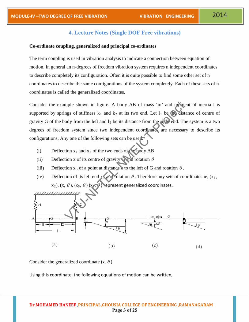
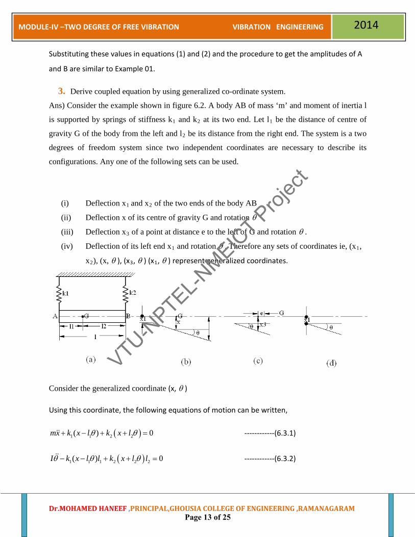
Consider the example shown in figure. A body AB of mass ‘m’ and moment of inertia l is

supported by springs of stiffness k1 and k2 at its two end. Let l1 be the distance of centre of

gravity G of the body from the left and l2 be its distance from the right end. The system is a two

degrees of freedom system since two independent coordinates are necessary to describe its

configurations. Any one of the following sets can be used.

(i) Deflection x1 and x2 of the two ends of the body AB

(ii) Deflection x of its centre of gravity G and rotation θ

(iii) Deflection x3 of a point at distance e to the left of G and rotation θ .

(iv) Deflection of its left end x1 and rotation θ . Therefore any sets of coordinates ie, (x1,

x2), (x, θ ), (x3, θ ) (x1, θ ) represent generalized coordinates.

Consider the generalized coordinate (x, θ )

Using this coordinate, the following equations of motion can be written,


VTU-NPTEL-N

MEICT Proj

ect

of 25


( )1 1 2 2( ) 0mx k x l k x lθ θ+ − + + = ------------(6.3.1)

( )1 1 1 2 2 2( ) 0I k x l l k x l lθ θ θ− − + + = ------------(6.3.2)

( )1 2 1 1 2 2( ) 0or mx k k x k l k l θ+ + − − = ------------(6.3.1)

( )2 21 1 2 2 1 1 2 2( ) 0I k l k l x k l k lθ θ− − + + = ------------(6.3.2)

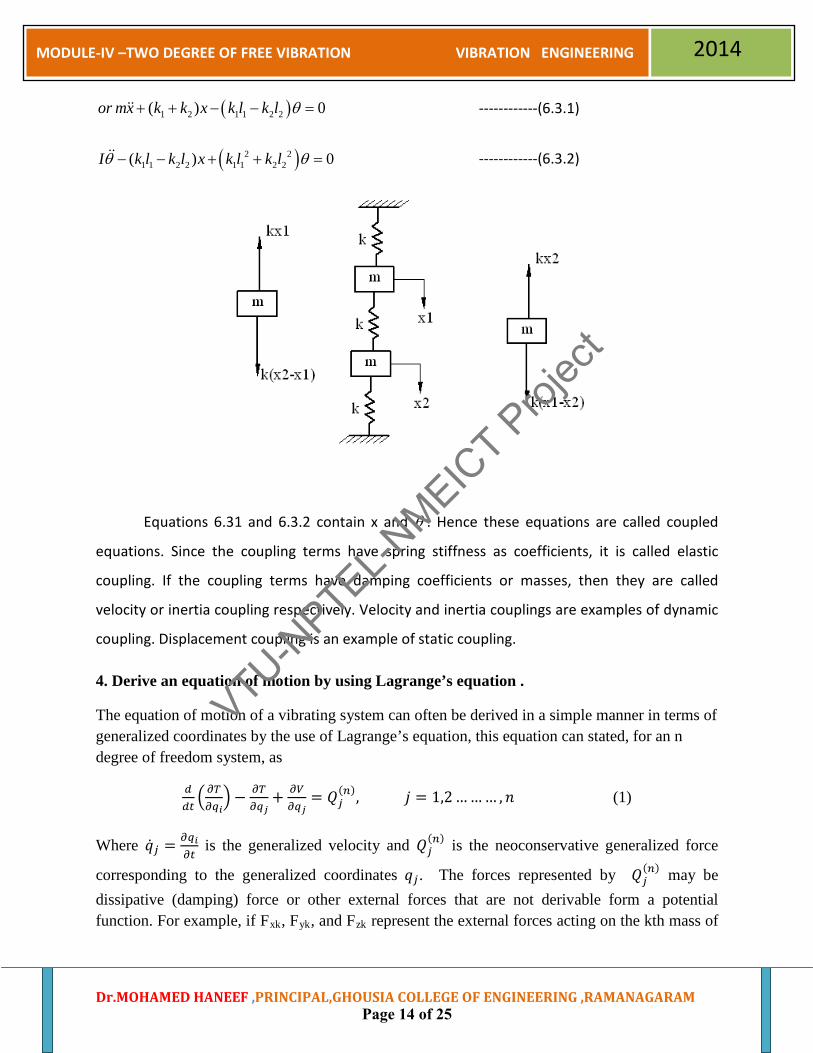
Equations 6.31 and 6.3.2 contain x and θ . Hence these equations are called coupled

equations. Since the coupling terms have spring stiffness as coefficients, it is called elastic

coupling. If the coupling terms have damping coefficients or masses, then they are called

velocity or inertia coupling respectively. Velocity and inertia couplings are examples of dynamic

coupling. Displacement coupling is an example of static coupling.

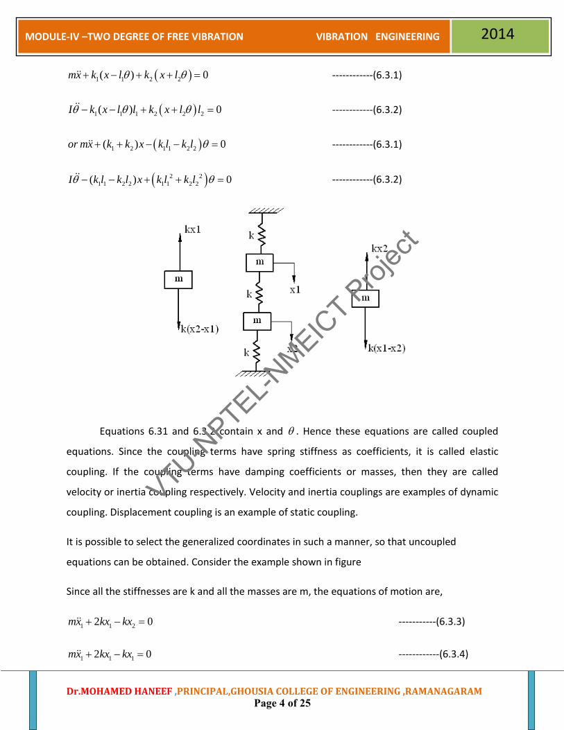
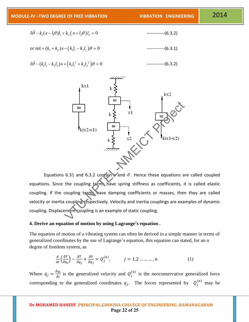
It is possible to select the generalized coordinates in such a manner, so that uncoupled

equations can be obtained. Consider the example shown in figure

Since all the stiffnesses are k and all the masses are m, the equations of motion are,

1 1 22 0mx kx kx+ − = -----------(6.3.3)

1 1 12 0mx kx kx+ − = ------------(6.3.4)


VTU-NPTEL-N

MEICT Proj

ect

of 25


Adding and subtracting the equations 6.3.3 and 6.3.4 we get

( )1 2 1 2( ) 0m x x k x x+ + + = ------------(6.3.5)

( )1 2 1 2( ) 3 0m x x k x x− + − = ------------(6.3.6)

If the generalized coordinates are,

p1 = x1 + x2 and p2 = x1 – x2

Equations 6.3.5 and 6.3.6 can be written as

1 1 0mp kp+ = -----------(6.3.7)

2 23 0mp kp+ = ------------(6.3.8)

Equations 6.3.7 and 6.3.8 are uncoupled equations. The set of coordinates (p1, p2) which result

in uncoupled equations are called principal coordinates.

Forced oscillations-Harmonic excitation

Consider the two degrees of freedom undamped system subjected to the harmonic forces as

shown in figure


VTU-NPTEL-N

MEICT Proj

ect

of 25


Fig. 6.46

The free body diagrams of the two masses are shown in figure 6.46 (b).

The harmonic forces acting on the systems are

F1(t) = F1 sin tω

F2(t) = F2 sin tω

The equations of motion are obtained from Newton’s second law of motion. Considering the

free body diagram shown in figure 6.46 (b), the equations are

( )1 1 1 2 1 2 1 sinm x k x k x x F tω= − − − −

i.e., 1 1 1 1 2 1 2 1( ) sinm x k x k x x F tω+ + − = ------------(6.6.1)

i.e., 1 1 1 2 1 2 2 1( ) sinm x k k x k x F tω+ + − =

Similarly 2 2 2 2 2 1 2 1( ) ( sin )m x k x k x x F tω+ − − − −

i.e., 2 2 2 2 2 1 1 sinm x k x k x F tω+ − = ------------(6.6.2)

Equations 6.6.1 and 6.6.2 are coupled and non-homogenous. Let the solutions of equations

6.6.1 and 6.6.2 be

( )( )

1

2

2 21 2

sin

sin

sin sin

x t A t

x t B t

x A t and x B t

ω

ω

ω ω ω ω

=

=

∴ = − = −

Substituting these values in equations 6.6.1 and 6.6.2

( ) ( )21 1 2 2 1sin sin sin sinm A t k k A t k B t F tω ω ω ω ω− + + − =

i.e., ( )21 1 2 2 1m k k A k B Fω − + + − =


VTU-NPTEL-N

MEICT Proj

ect

of 25


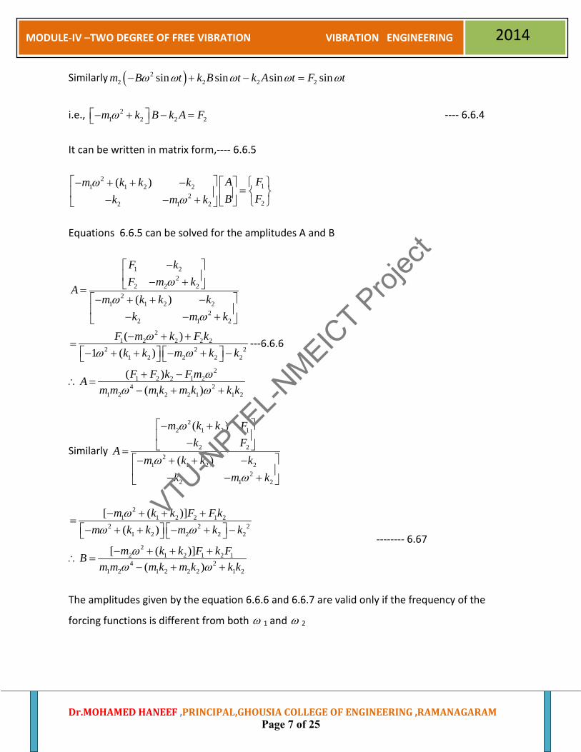
Similarly ( )22 2 2 2sin sin sin sinm B t k B t k A t F tω ω ω ω ω− + − =

i.e., 21 2 2 2m k B k A Fω − + − = ---- 6.6.4

It can be written in matrix form,---- 6.6.5

211 1 2 2

222 1 2

( ) FAm k k kFBk m k

ωω

− + + − = − − +

Equations 6.6.5 can be solved for the amplitudes A and B

1 22

2 2 22

1 1 2 22

2 1 2

21 2 2 2 2

2 2 21 2 2 2 2

21 2 2 1 2

4 21 2 1 2 2 1 1 2

( )

( )1 ( )

( )( )

F kF m k

Am k k k

k m k

F m k F kk k m k k

F F k F mAm m m k m k k k

ωω

ω

ωω ω

ωω ω

− − + =

− + + − − − +

− + += − + + − + −

+ −∴ =

− + +

---6.6.6

Similarly

22 1 2 1

2 22

1 1 2 22

2 1 2

( )

( )

m k k Fk F

Am k k k

k m k

ω

ωω

− + − =

− + + − − − +

21 1 2 2 1 2

2 2 21 2 2 2 2

22 1 2 1 2 14 2

1 2 1 2 2 2 1 2

[ ( )]( )

[ ( )]( )

m k k F F km k k m k k

m k k F k FBm m m k m k k k

ωω ω

ωω ω

− + + += − + + − + −

− + + +∴ =

− + +

-------- 6.67

The amplitudes given by the equation 6.6.6 and 6.6.7 are valid only if the frequency of the

forcing functions is different from both ω 1 and ω 2


VTU-NPTEL-N

MEICT Proj

ect

of 25


From above figure , a complex equation can be represented by,

(cos sin ) i tx A t i t Ae ωω ω= + =

Hence the steady state responses for the two masses m1 and m2 are given by the imaginary

parts of

A i te ω and B i te ω respectively,

The steady state responses are,

21 2 2 1 2 1

1 4 21 2 1 2 2 2 2 1 1 2

( )( ) .sin( )F F k F mx t t

m m m k m k m k k kω ω

ω ω+ −

=− + + +

------ 6.6.8

21 1 2 1 2 1

2 4 21 2 1 2 2 2 2 1 1 2

( )( ) .sin

( )m k k F k F

x t tm m m k m k m k k k

ωω

ω ω

− + + + =− + + +

------6.6.9


VTU-NPTEL-N

MEICT Proj

ect

of 25


QUADRANT-2

Animations (Animations related, Two degree of Free Vibration)

• http://acoustics.mie.uic.edu/Simulation/Index.htm • http://acoustics.mie.uic.edu/Simulation/Mass_Spring_2DOF.htm • http://www.acs.psu.edu/drussell/demos.html • http://www.acs.psu.edu/drussell/Demos/SHO/mass-force.html

Videos (Videos links related, Two degree of Free Vibration)

• http://www.youtube.com/watch?v=6gX4ox-r5t0 • http://www.youtube.com/watch?v=904QIyzM29o • http://freevideolectures.com/Course/2364/Dynamics-of-Machines/32 • http://freevideolectures.com/Course/2684/Mechanical-Vibrations/13 • http://www.cosmolearning.com/video-lectures/generalized-and-principle-coordinates-

derivation-of-equation-of-motion-11545/ • http://www.youtube.com/watch?v=AN8Ip39LXJg • http://freevideolectures.com/Course/2286/Artificial-Intelligence-Introduction-to-Robotics/12 • http://videolectures.net/stanfordcs223aw08_khatib_lec12/ • http://www.youtube.com/watch?v=G6OX1NpToaw • http://www.youtube.com/watch?v=FYCII12btS4 • http://www.youtube.com/watch?v=ruR8Gfm0khc • http://freevideolectures.com/Course/2684/Mechanical-Vibrations/15 • http://www.youtube.com/watch?v=Q_MkjK29_Vg • http://www.cosmolearning.com/video-lectures/coordinate-coupling-11547/ • http://mechanical-engineering.in/forum/videos/view-497-lecture-15-mod-5-lec-3-coordinate-

coupling/ • http://www.youtube.com/watch?v=GFd-uHttAeU • http://www.youtube.com/watch?v=zQ0mRAjy2vM • http://freevideolectures.com/Course/2684/Mechanical-Vibrations/8


VTU-NPTEL-N

MEICT Proj

ect

of 25

http://acoustics.mie.uic.edu/Simulation/Index.htm

http://acoustics.mie.uic.edu/Simulation/Mass_Spring_2DOF.htm

http://www.acs.psu.edu/drussell/demos.html

http://www.acs.psu.edu/drussell/Demos/SHO/mass-force.html

http://www.youtube.com/watch?v=6gX4ox-r5t0

http://www.youtube.com/watch?v=904QIyzM29o

http://freevideolectures.com/Course/2364/Dynamics-of-Machines/32

http://freevideolectures.com/Course/2684/Mechanical-Vibrations/13

http://www.cosmolearning.com/video-lectures/generalized-and-principle-coordinates-derivation-of-equation-of-motion-11545/

http://www.cosmolearning.com/video-lectures/generalized-and-principle-coordinates-derivation-of-equation-of-motion-11545/

http://www.youtube.com/watch?v=AN8Ip39LXJg

http://freevideolectures.com/Course/2286/Artificial-Intelligence-Introduction-to-Robotics/12

http://videolectures.net/stanfordcs223aw08_khatib_lec12/

http://www.youtube.com/watch?v=G6OX1NpToaw

http://www.youtube.com/watch?v=FYCII12btS4

http://www.youtube.com/watch?v=ruR8Gfm0khc


http://www.youtube.com/watch?v=Q_MkjK29_Vg

http://www.cosmolearning.com/video-lectures/coordinate-coupling-11547/

http://mechanical-engineering.in/forum/videos/view-497-lecture-15-mod-5-lec-3-coordinate-coupling/

http://mechanical-engineering.in/forum/videos/view-497-lecture-15-mod-5-lec-3-coordinate-coupling/

http://www.youtube.com/watch?v=GFd-uHttAeU

http://www.youtube.com/watch?v=zQ0mRAjy2vM



ILLUSTRATIONS

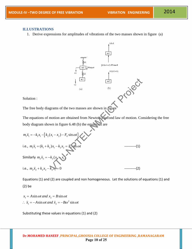
1. Derive expressions for amplitudes of vibrations of the two masses shown in figure (a)

Solution :

The free body diagrams of the two masses are shown in figure

The equations of motion are obtained from Newton’s second law of motion. Considering the free

body diagram shown in figure 6.48 (b) the equations are

[ ]1 1 1 1 2 1 2 0( ) sinm x k x k x x F tω= − − − −

i.e., 1 1 1 2 1 2 2 0( ) sinm x k k x k x F tω= + − = ----------(1)

Similarly 2 2 2 2 1( )m x k x x= − −

i.e., 2 2 2 2 2 1 0m x k x k x+ − = ----------(2)

Equations (1) and (2) are coupled and non homogeneous. Let the solutions of equations (1) and

(2) be

1 22

1 2

sin sinsin sin

x A t and x B tx A t and x B t

ω ω

ω ω ω

= =

∴ = − = −

Substituting these values in equations (1) and (2)


VTU-NPTEL-N

MEICT Proj

ect

of 25


21 1 2 2 0sin ( ) sin sin sinm A t k k A t k B t F tω ω ω ω ω− + + − =

i.e., 21 1 2 2 0( )m k k A k B Fω − + + − = -------- (3)

Similarly 21 2 2sin sin sin 0m B t k B t k A tω ω ω ω− + − = ------------ (4)

i.e., 21 2 2( ) 0m k B k Aω− + − =

It can be written in matrix form

201 1 2 2

22 1 2

( )0

A Fm k k kBk m k

ωω

− + + − = − − +

------------ (5)

Equation (5) can be solved for the amplitudes A and B.

0 22

2 22

1 1 2 22

2 1 2

20 2 2

4 21 2 1 2 2 2 2 1 1 2

0( )

( )( )

F km k

Am k k k

k m k

F k mm m m k m k m k k k

ωω

ω

ωω ω

− − + ∴ =

− + + − − − +

+ −=

− + + +

------------ (6)

Similarly,

22 1 2 0

22

1 1 2 22

2 1 2

0 24 2

1 2 1 2 2 2 2 1 1 2

( )0

( )

( )

m k k Fk

Bm k k k

k m kF k

m m m k m k m k k k

ω

ωω

ω ω

− + − =

− + + − − − +

=− + + +

------------ (7)


VTU-NPTEL-N

MEICT Proj

ect

of 25


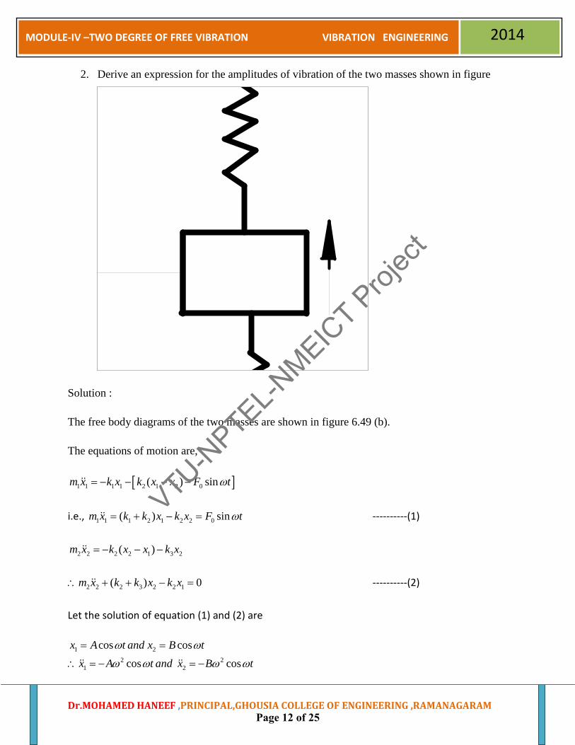
2. Derive an expression for the amplitudes of vibration of the two masses shown in figure

Solution :


The equations of motion are,

[ ]1 1 1 1 2 1 2 0( ) sinm x k x k x x F tω= − − − −


2 2 2 2 1 3 2( )m x k x x k x= − − −

2 2 2 3 2 2 1( ) 0m x k k x k x∴ + + − = ----------(2)

Let the solution of equation (1) and (2) are

1 22 2

1 2

cos coscos cos


ω ω

ω ω ω ω

= =

∴ = − = −


VTU-NPTEL-N

MEICT Proj

ect

of 25


Substituting these values in equations (1) and (2) and the procedure to get the amplitudes of A

and B are similar to Example 01.

3. Derive coupled equation by using generalized co-ordinate system. Ans) Consider the example shown in figure 6.2. A body AB of mass ‘m’ and moment of inertia l

is supported by springs of stiffness k1 and k2 at its two end. Let l1 be the distance of centre of




(i) Deflection x1 and x2 of the two ends of the body AB

(ii) Deflection x of its centre of gravity G and rotation θ

(iii) Deflection x3 of a point at distance e to the left of G and rotation θ .

(iv) Deflection of its left end x1 and rotation θ . Therefore any sets of coordinates ie, (x1,




( )1 1 2 2( ) 0mx k x l k x lθ θ+ − + + = ------------(6.3.1)

( )1 1 1 2 2 2( ) 0I k x l l k x l lθ θ θ− − + + = ------------(6.3.2)


VTU-NPTEL-N

MEICT Proj

ect

of 25


( )1 2 1 1 2 2( ) 0or mx k k x k l k l θ+ + − − = ------------(6.3.1)

( )2 21 1 2 2 1 1 2 2( ) 0I k l k l x k l k lθ θ− − + + = ------------(6.3.2)






4. Derive an equation of motion by using Lagrange’s equation .

The equation of motion of a vibrating system can often be derived in a simple manner in terms of generalized coordinates by the use of Lagrange’s equation, this equation can stated, for an n degree of freedom system, as

𝑑𝑑𝑡�𝜕𝑇𝜕𝑞𝑖� − 𝜕𝑇

𝜕𝑞𝑗+ 𝜕𝑉

𝜕𝑞𝑗= 𝑄𝑗

(𝑛), 𝑗 = 1,2 … … … ,𝑛 (1)

Where �̇�𝑗 = 𝜕𝑞𝑖𝜕𝑡

is the generalized velocity and 𝑄𝑗(𝑛) is the neoconservative generalized force

corresponding to the generalized coordinates 𝑞𝑗. The forces represented by 𝑄𝑗(𝑛) may be

dissipative (damping) force or other external forces that are not derivable form a potential function. For example, if Fxk, Fyk, and Fzk represent the external forces acting on the kth mass of


VTU-NPTEL-N

MEICT Proj

ect

of 25


the system in the x, y, and z directions, respectively, then the generalized force Qj(n) can be

computed as follows:

𝑄𝑗(𝑛) = ∑ � 𝐹𝑥𝑘

𝜕𝑥𝑘𝜕𝑞𝑗

+ 𝐹𝑦𝑘𝜕𝑦𝑘𝜕𝑞𝑗

+ 𝐹𝑧𝑘𝜕𝑧𝑘𝜕𝑞𝑗�𝑘 (2)

Where xk, yk, zk are the displacements of the kth mass in the x, y and z directions, respectively. Note that for a torsional system, the force Fxk, for example, is to be replaced by the moment acting about the x axis (Mxk), and the displacement xk by the angular displacement about the x axis (θxk) in equation (2). For a conservative system, 𝑄𝑗

(𝑛) = 0, so equation (1) takes the form



𝜕𝑞𝑗= 0, 𝑗 = 1,2 … … … ,𝑛 (3)

Equations (1) or (3) represent a system of n differential equations, one corresponding to each of the n generalized coordinates. Thus the equations of motion of the vibrating system can be derived, provided the energy expressions are available.

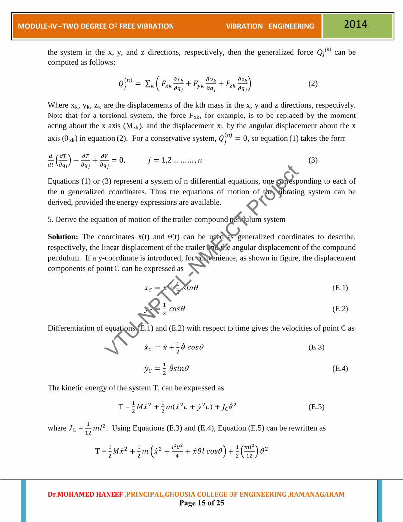
5. Derive the equation of motion of the trailer-compound pendulum system

Solution: The coordinates x(t) and θ(t) can be used as generalized coordinates to describe, respectively, the linear displacement of the trailer and the angular displacement of the compound pendulum. If a y-coordinate is introduced, for convenience, as shown in figure, the displacement components of point C can be expressed as

𝑥𝐶 = 𝑥 + 12

𝑠𝑖𝑛θ (E.1)

𝑦𝐶 = 12

𝑐𝑜𝑠θ (E.2)

Differentiation of equations (E.1) and (E.2) with respect to time gives the velocities of point C as

�̇�𝐶 = �̇� + 12�̇� 𝑐𝑜𝑠θ (E.3)

�̇�𝐶 = 12

�̇�𝑠𝑖𝑛θ (E.4)

The kinetic energy of the system T, can be expressed as

T = 12𝑀�̇�2 + 1

2𝑚(�̇�2𝑐 + �̇�2𝑐) + 𝐽𝐶�̇�2 (E.5)

where JC = 112𝑚𝑙2. Using Equations (E.3) and (E.4), Equation (E.5) can be rewritten as

T = 12𝑀�̇�2 + 1

2𝑚 ��̇�2 + 𝑙2�̇�2

4+ �̇��̇�𝑙 𝑐𝑜𝑠𝜃� + 1

2�𝑚𝑙2

12� �̇�2


VTU-NPTEL-N

MEICT Proj

ect

of 25


= 12

(𝑀 + 𝑚)�̇�2 + 12�𝑚𝑙2

3� �̇�2 + 1

2(𝑚𝑙 𝑐𝑜𝑠𝜃) �̇��̇� (E.6)

The potential energy of the system, V, due to the strain energy of the springs and the gravitational potential, can be expressed as

V = 12𝑘1𝑥2 + 1

2𝑘2𝑥2 + 𝑚𝑔 𝑙

2(1 − 𝑐𝑜𝑠𝜃) (E.7)

where the lowest position of point C is taken as the datum. Since there are nonconservative forces acting on the system, the generalized forces corresponding to x(t) and θ(t) are to be computed. The force, X(t), acting in the direction of x(t) can be found from Equation (2) as

X(t) = 𝑄𝑗(𝑛) = 𝐹(𝑡) − 𝑐1�̇�(𝑡) − 𝑐2�̇�(𝑡) (E.8)

where the negative sign for the terms 𝑐1�̇� and 𝑐2�̇� indicates that the damping forces oppose the motion. Similarly, the force Θ(t) acting in the direction of θ(t) can be determined as

Θ(t) = 𝑄2(𝑛) = 𝑀𝑡(𝑡) (E.9)

where q1 = x and q2 = θ. By differentiating the expressions of T and V as required by Equations (1) and substituting the resulting expressions, along with Equations (E.8) and (E.9), we obtain the equations of motion of the system as

(𝑀 = 𝑚)�̈� +12

(𝑚𝑙 𝑐𝑜𝑠𝜃)�̈� −12𝑚𝑙 sin𝜃�̇�2 + 𝑘1𝑥 + 𝑘2𝑥

= 𝐹(𝑡) − 𝑐1�̇� − 𝑐2�̇� (E.10)

�13𝑚𝑙2� �̈� + 1

2(𝑚𝑙 𝑐𝑜𝑠𝜃)�̈� − 1

2𝑚𝑙𝑠𝑖𝑛𝜃�̇��̇� + 1

2𝑚𝑙𝑠𝑖𝑛𝜃�̇��̇�

+𝑚𝑔𝑙 𝑠𝑖𝑛𝜃 = 𝑀𝑡(𝑡) (E.11)

Equations (E.10) and (E.11) can be seen to be identical to those obtained using Newton’s second law of motion (Equations E.1 and E.2 in Example 6.2).


VTU-NPTEL-N

MEICT Proj

ect

of 25


QUADRANT-3

Wikis: (This includes wikis related to Two degree of Free Vibration)

• http://en.wikipedia.org/wiki/Vibration • http://wikis.controltheorypro.com/Vibration_in_Systems_with_Two_Degrees_of_Freedom

Open Contents: (This includes wikis related to Finite Element Analysis)

• Mechanical Vibrations, S. S. Rao, Pearson Education Inc, 4th edition, 2003. • Mechanical Vibrations, V. P. Singh, Dhanpat Rai & Company, 3rd edition, 2006. • Mechanical Vibrations, G. K.Grover, Nem Chand and Bros, 6th edition, 1996 • Theory of vibration with applications ,W.T.Thomson,M.D.Dahleh and C

Padmanabhan,Pearson Education inc,5th Edition ,2008 • Theory and practice of Mechanical Vibration : J.S.Rao&K,Gupta,New Age International

Publications ,New Delhi,2001 • Fintie Elemeent Methods by Mrugendrappa, S B Halesh, Manohar • A Mechanical Vibration by Hamelton


VTU-NPTEL-N

MEICT Proj

ect

of 25

http://en.wikipedia.org/wiki/Vibration

http://wikis.controltheorypro.com/Vibration_in_Systems_with_Two_Degrees_of_Freedom


QUADRANT-4 Frequently asked Questions.

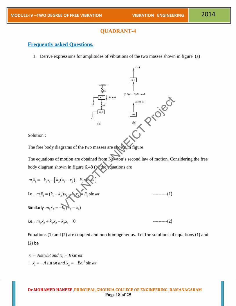
1. Derive expressions for amplitudes of vibrations of the two masses shown in figure (a)

Solution :

The free body diagrams of the two masses are shown in figure

The equations of motion are obtained from Newton’s second law of motion. Considering the free

body diagram shown in figure 6.48 (b) the equations are

[ ]1 1 1 1 2 1 2 0( ) sinm x k x k x x F tω= − − − −


Similarly 2 2 2 2 1( )m x k x x= − −

i.e., 2 2 2 2 2 1 0m x k x k x+ − = ----------(2)

Equations (1) and (2) are coupled and non homogeneous. Let the solutions of equations (1) and

(2) be

1 22

1 2

sin sinsin sin


ω ω

ω ω ω

= =

∴ = − = −


VTU-NPTEL-N

MEICT Proj

ect

of 25


Substituting these values in equations (1) and (2)

21 1 2 2 0sin ( ) sin sin sinm A t k k A t k B t F tω ω ω ω ω− + + − =

i.e., 21 1 2 2 0( )m k k A k B Fω − + + − = -------- (3)

Similarly 21 2 2sin sin sin 0m B t k B t k A tω ω ω ω− + − = ------------ (4)

i.e., 21 2 2( ) 0m k B k Aω− + − =

It can be written in matrix form

201 1 2 2

22 1 2

( )0

A Fm k k kBk m k

ωω

− + + − = − − +

------------ (5)

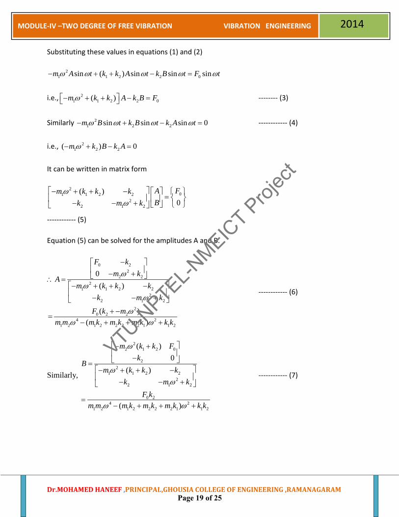
Equation (5) can be solved for the amplitudes A and B.

0 22

2 22

1 1 2 22

2 1 2

20 2 2

4 21 2 1 2 2 2 2 1 1 2

0( )

( )( )

F km k

Am k k k

k m k

F k mm m m k m k m k k k

ωω

ω

ωω ω

− − + ∴ =

− + + − − − +

+ −=

− + + +

------------ (6)

Similarly,

22 1 2 0

22

1 1 2 22

2 1 2

0 24 2

1 2 1 2 2 2 2 1 1 2

( )0

( )

( )

m k k Fk

Bm k k k

k m kF k

m m m k m k m k k k

ω

ωω

ω ω

− + − =

− + + − − − +

=− + + +

------------ (7)


VTU-NPTEL-N

MEICT Proj

ect

of 25


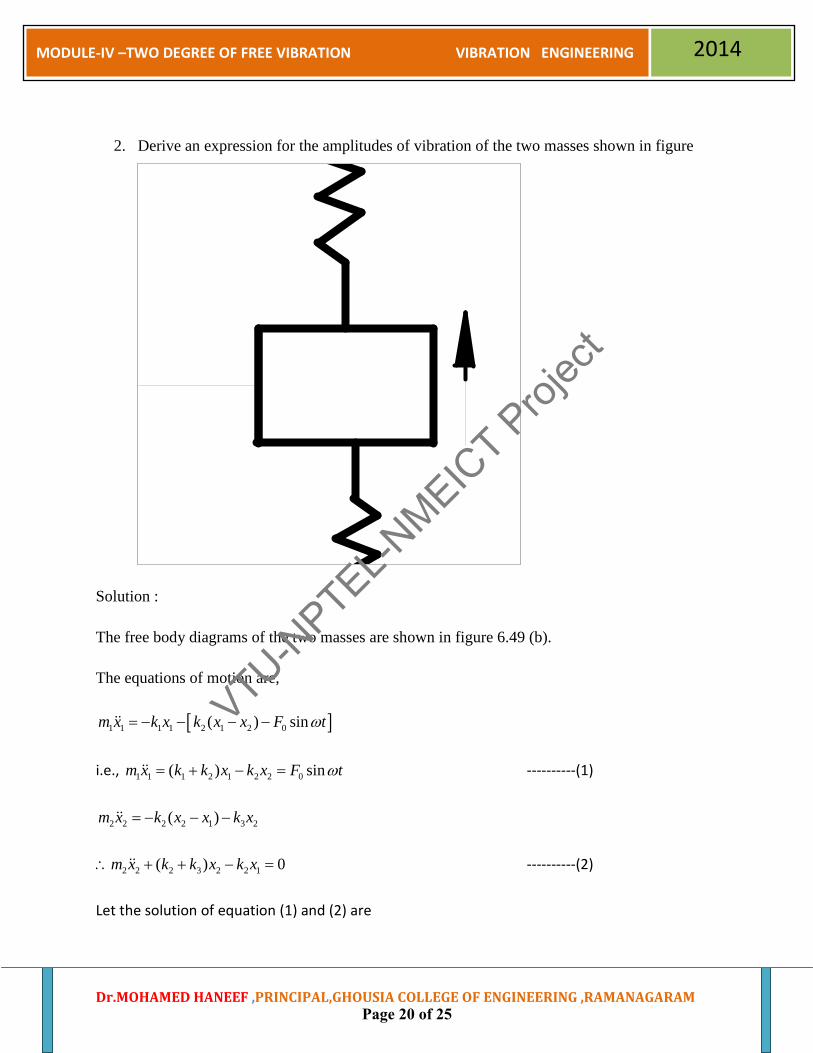
2. Derive an expression for the amplitudes of vibration of the two masses shown in figure

Solution :


The equations of motion are,

[ ]1 1 1 1 2 1 2 0( ) sinm x k x k x x F tω= − − − −


2 2 2 2 1 3 2( )m x k x x k x= − − −

2 2 2 3 2 2 1( ) 0m x k k x k x∴ + + − = ----------(2)

Let the solution of equation (1) and (2) are


VTU-NPTEL-N

MEICT Proj

ect

of 25


1 22 2

1 2

cos coscos cos


ω ω

ω ω ω ω

= =

∴ = − = −

Substituting these values in equations (1) and (2) and the procedure to get the amplitudes of A

and B are similar to Example 01.

3. Derive coupled equation by using generalized co-ordinate system. Ans) Consider the example shown in figure 6.2. A body AB of mass ‘m’ and moment of inertia l

is supported by springs of stiffness k1 and k2 at its two end. Let l1 be the distance of centre of




(v) Deflection x1 and x2 of the two ends of the body AB

(vi) Deflection x of its centre of gravity G and rotation θ

(vii) Deflection x3 of a point at distance e to the left of G and rotation θ .

(viii) Deflection of its left end x1 and rotation θ . Therefore any sets of coordinates ie, (x1,




( )1 1 2 2( ) 0mx k x l k x lθ θ+ − + + = ------------(6.3.1)


VTU-NPTEL-N

MEICT Proj

ect

of 25


( )1 1 1 2 2 2( ) 0I k x l l k x l lθ θ θ− − + + = ------------(6.3.2)

( )1 2 1 1 2 2( ) 0or mx k k x k l k l θ+ + − − = ------------(6.3.1)

( )2 21 1 2 2 1 1 2 2( ) 0I k l k l x k l k lθ θ− − + + = ------------(6.3.2)






4. Derive an equation of motion by using Lagrange’s equation .

The equation of motion of a vibrating system can often be derived in a simple manner in terms of generalized coordinates by the use of Lagrange’s equation, this equation can stated, for an n degree of freedom system, as



𝜕𝑞𝑗= 𝑄𝑗

(𝑛), 𝑗 = 1,2 … … … ,𝑛 (1)

Where �̇�𝑗 = 𝜕𝑞𝑖𝜕𝑡

is the generalized velocity and 𝑄𝑗(𝑛) is the neoconservative generalized force

corresponding to the generalized coordinates 𝑞𝑗. The forces represented by 𝑄𝑗(𝑛) may be


VTU-NPTEL-N

MEICT Proj

ect

of 25


dissipative (damping) force or other external forces that are not derivable form a potential function. For example, if Fxk, Fyk, and Fzk represent the external forces acting on the kth mass of the system in the x, y, and z directions, respectively, then the generalized force Qj

(n) can be computed as follows:

𝑄𝑗(𝑛) = ∑ � 𝐹𝑥𝑘

𝜕𝑥𝑘𝜕𝑞𝑗

+ 𝐹𝑦𝑘𝜕𝑦𝑘𝜕𝑞𝑗

+ 𝐹𝑧𝑘𝜕𝑧𝑘𝜕𝑞𝑗�𝑘 (2)

Where xk, yk, zk are the displacements of the kth mass in the x, y and z directions, respectively. Note that for a torsional system, the force Fxk, for example, is to be replaced by the moment acting about the x axis (Mxk), and the displacement xk by the angular displacement about the x axis (θxk) in equation (2). For a conservative system, 𝑄𝑗

(𝑛) = 0, so equation (1) takes the form



𝜕𝑞𝑗= 0, 𝑗 = 1,2 … … … ,𝑛 (3)

Equations (1) or (3) represent a system of n differential equations, one corresponding to each of the n generalized coordinates. Thus the equations of motion of the vibrating system can be derived, provided the energy expressions are available.

5. Derive the equation of motion of the trailer-compound pendulum system

Solution: The coordinates x(t) and θ(t) can be used as generalized coordinates to describe, respectively, the linear displacement of the trailer and the angular displacement of the compound pendulum. If a y-coordinate is introduced, for convenience, as shown in figure, the displacement components of point C can be expressed as

𝑥𝐶 = 𝑥 + 12

𝑠𝑖𝑛θ (E.1)

𝑦𝐶 = 12

𝑐𝑜𝑠θ (E.2)

Differentiation of equations (E.1) and (E.2) with respect to time gives the velocities of point C as

�̇�𝐶 = �̇� + 12�̇� 𝑐𝑜𝑠θ (E.3)

�̇�𝐶 = 12

�̇�𝑠𝑖𝑛θ (E.4)

The kinetic energy of the system T, can be expressed as

T = 12𝑀�̇�2 + 1

2𝑚(�̇�2𝑐 + �̇�2𝑐) + 𝐽𝐶�̇�2 (E.5)

where JC = 112𝑚𝑙2. Using Equations (E.3) and (E.4), Equation (E.5) can be rewritten as


VTU-NPTEL-N

MEICT Proj

ect

of 25


T = 12𝑀�̇�2 + 1

2𝑚 ��̇�2 + 𝑙2�̇�2

4+ �̇��̇�𝑙 𝑐𝑜𝑠𝜃� + 1

2�𝑚𝑙2

12� �̇�2

= 12

(𝑀 + 𝑚)�̇�2 + 12�𝑚𝑙2

3� �̇�2 + 1

2(𝑚𝑙 𝑐𝑜𝑠𝜃) �̇��̇� (E.6)

The potential energy of the system, V, due to the strain energy of the springs and the gravitational potential, can be expressed as

V = 12𝑘1𝑥2 + 1

2𝑘2𝑥2 + 𝑚𝑔 𝑙

2(1 − 𝑐𝑜𝑠𝜃) (E.7)

where the lowest position of point C is taken as the datum. Since there are nonconservative forces acting on the system, the generalized forces corresponding to x(t) and θ(t) are to be computed. The force, X(t), acting in the direction of x(t) can be found from Equation (2) as

X(t) = 𝑄𝑗(𝑛) = 𝐹(𝑡) − 𝑐1�̇�(𝑡) − 𝑐2�̇�(𝑡) (E.8)

where the negative sign for the terms 𝑐1�̇� and 𝑐2�̇� indicates that the damping forces oppose the motion. Similarly, the force Θ(t) acting in the direction of θ(t) can be determined as

Θ(t) = 𝑄2(𝑛) = 𝑀𝑡(𝑡) (E.9)

where q1 = x and q2 = θ. By differentiating the expressions of T and V as required by Equations (1) and substituting the resulting expressions, along with Equations (E.8) and (E.9), we obtain the equations of motion of the system as

(𝑀 = 𝑚)�̈� +12

(𝑚𝑙 𝑐𝑜𝑠𝜃)�̈� −12𝑚𝑙 sin𝜃�̇�2 + 𝑘1𝑥 + 𝑘2𝑥

= 𝐹(𝑡) − 𝑐1�̇� − 𝑐2�̇� (E.10)

�13𝑚𝑙2� �̈� + 1

2(𝑚𝑙 𝑐𝑜𝑠𝜃)�̈� − 1

2𝑚𝑙𝑠𝑖𝑛𝜃�̇��̇� + 1

2𝑚𝑙𝑠𝑖𝑛𝜃�̇��̇�

+𝑚𝑔𝑙 𝑠𝑖𝑛𝜃 = 𝑀𝑡(𝑡) (E.11)

Equations (E.10) and (E.11) can be seen to be identical to those obtained using Newton’s second law of motion (Equations E.1 and E.2 in Example 6.2).

Assignment : 1. Define two degrees of freedom? Give an example on two DOF free vibrations. 2. Explain the following:


VTU-NPTEL-N

MEICT Proj

ect

of 25


a) Generalized & principle coordinates. b) Coordinates coupling.

3. Drive an equation of motion by using generalized & principle coordinates. 4. Explain Lagrange’s equation. 5. Explain forced harmonic vibration by using an Example. 6. Derive an equation of motion for forced harmonic vibration by using simple two DOF

spring-mass systems. 7. Consider a double pendulum (two DOF) assume l1 = l & l2 = 2l, m1 = m2 =m. obtain the

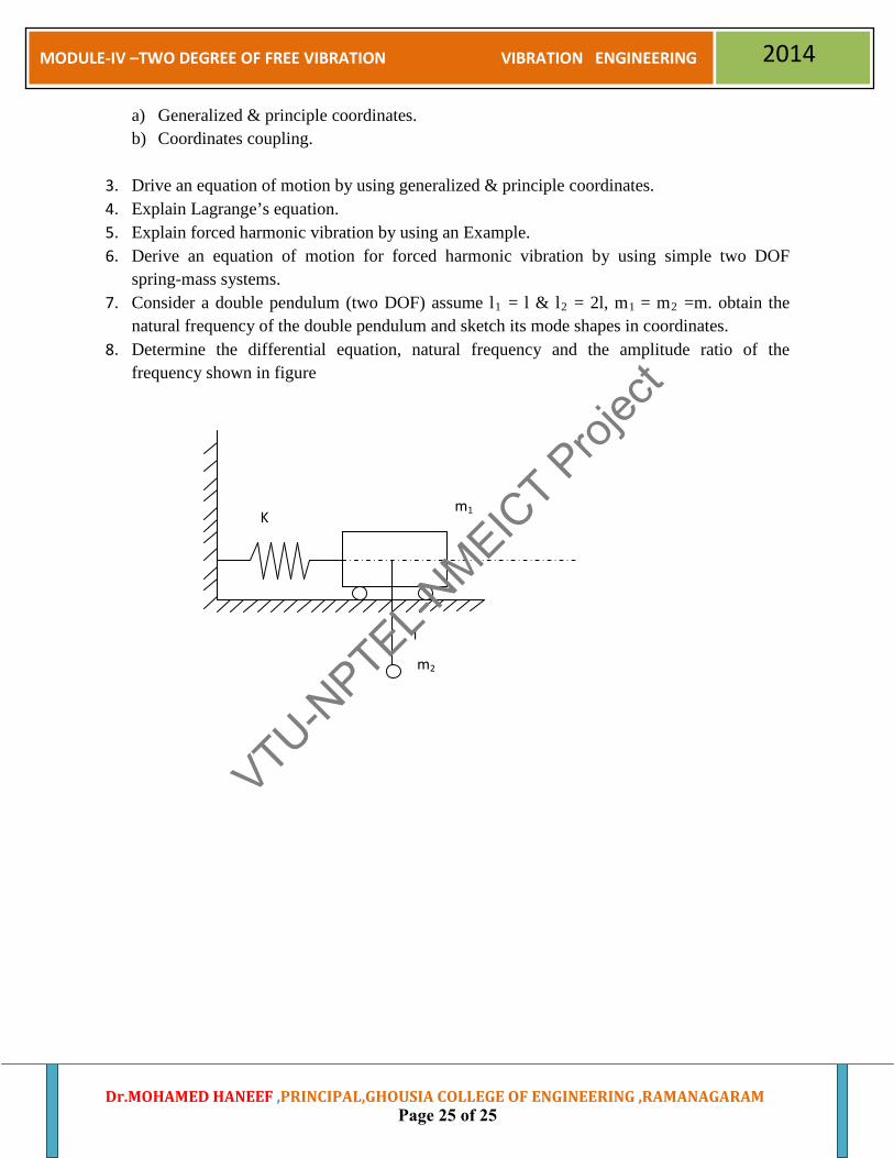
natural frequency of the double pendulum and sketch its mode shapes in coordinates. 8. Determine the differential equation, natural frequency and the amplitude ratio of the

frequency shown in figure

m2

m1 K

l


VTU-NPTEL-N

MEICT Proj

ect

of 25

subject matter expert details vtu-ntel-nmeict rojectnptel.vtu.ac.in/vtu-nmeict/mv/module 4.pdf ·...

Documents