study of the dynamics of streamers in air at atmospheric pressure
TRANSCRIPT
HAL Id: tel-00463743https://tel.archives-ouvertes.fr/tel-00463743
Submitted on 15 Mar 2010
HAL is a multi-disciplinary open accessarchive for the deposit and dissemination of sci-entific research documents, whether they are pub-lished or not. The documents may come fromteaching and research institutions in France orabroad, or from public or private research centers.
L’archive ouverte pluridisciplinaire HAL, estdestinée au dépôt et à la diffusion de documentsscientifiques de niveau recherche, publiés ou non,émanant des établissements d’enseignement et derecherche français ou étrangers, des laboratoirespublics ou privés.
Study of the dynamics of streamers in air atatmospheric pressure
Sébastien Célestin
To cite this version:Sébastien Célestin. Study of the dynamics of streamers in air at atmospheric pressure. EngineeringSciences [physics]. Ecole Centrale Paris, 2008. English. <tel-00463743>
École Centrale Paris
THÈSE
présentée par
Sébastien Célestin
pour l’obtention du
GRADE de DOCTEUR
Formation doctorale : Physique
Laboratoire d’accueil : Laboratoire d’Energétique Moléculaire et Macroscopique,Combustion (EM2C) du CNRS et de l’ECP
Study of the dynamics of streamers in air atatmospheric pressure
Soutenue le 8 Décembre 2008
Composition du jury : MM. Boeuf J.-P. ReviewerBourdon A. AdvisorHassouni K. ReviewerPaillol J.-H.Pasko V.Rousseau A. Co-advisorSégur P.Starikovskaia S.
École Centrale des Arts et ManufacturesGrand Etablissement sous tutelledu Ministère de l’Education NationaleGrande Voie des Vignes92295 CHATENAY MALABRY CedexTél. : 33 (1) 41 13 10 00 (standard)Télex : 634 991 F EC PARIS
Laboratoire d’Énergétique Moléculaireet Macroscopique, Combustion (E.M2.C.)UPR 288, CNRS et École Centrale ParisTél. : 33 (1) 41 13 10 31Fax : 33 (1) 47 02 80 35
2008 - 53

Résumé
Dans cette thèse, nous avons étudié d’un point de vue expérimental et numérique la dy-namique et la structure des décharges de type streamer dans l’air à la pression atmo-sphérique. Deux configurations ont été étudiées: une décharge Nanoseconde RépétitivePulsée (NRP) entre deux pointes dans l’air préchauffé et une Décharge à Barrière Diélec-trique (DBD) dans une configuration pointe-plan. Nous avons montré que les simulationsde la dynamique de ces décharges sur des temps courts permettent d’obtenir des infor-mations sur la structure et les propriétés de ces décharges observées expérimentalement,généralement sur des temps plus longs. Dans le cadre de cette thèse, du point de vue dela simulation des décharges, deux nouvelles approches ont été développées: pour le calculde la photoionisation et pour la prise en compte d’électrodes de forme complexe dans desmaillages cartésiens.
Pour le calcul de la photoionisation dans l’air, le modèle intégral de référence requiertde longs temps de calcul. Dans ce travail, afin d’éviter de lourds calculs intégraux, nousavons développé plusieurs modèles différentiels qui permettent de prendre en compte ladépendance spectrale de la photoionisation, tout en restant simples et peu coûteux entemps de calcul. Parmi les modèles développés, nous avons montré que le modèle appeléSP3 3-groupes basé sur une approximation d’ordre 3 de l’équation de transfert radiatif étaitplus précis pour la simulation des streamers.
Afin de prendre en compte des électrodes de forme complexe dans les simulations, nous avonsadapté une méthode GFM (“Ghost Fluid Method”) pour résoudre l’équation de Poissonafin de calculer précisément le potentiel et le champ électrique près de l’électrode. Cetteméthode nous permet de prendre en compte l’influence de la forme exacte de l’électrodedans un maillage régulier, et ce quelque soit la forme de l’électrode.
Nous avons réalisé des simulations en géométrie pointe-pointe étroitement liées à de récentstravaux expérimentaux concernant des décharges générées par NRP dans de l’air préchauffé.Nous avons étudié la dynamique de la décharge dans l’espace inter-électrode pour différentestempératures de l’air et différentes tensions appliquées. Nous avons montré que la structurede la décharge dépendait fortement de la tension appliquée, ce qui est en bon accord avecles expériences.
Dans la partie expérimentale de ce travail, nous avons étudié un comportement particulierdes filaments de plasma dans une DBD pendant la demi-alternance positive de la ten-sion appliquée. La dynamique des décharges est fortement affectée par la charge de surfacedéposée sur le diélectrique. Nous avons simulé une configuration pointe-plan avec un diélec-trique plan sur la cathode dans le but de mieux comprendre l’influence de l’accumulationde la charge de surface sur l’allumage et la propagation de décharges successives dans uneDBD. Dans ce travail, nous avons simulé la propagation d’un streamer initié près de l’anodejusqu’au diélectrique, ainsi que la formation d’une décharge de surface sur celui-ci. Nousavons ainsi déterminé les échelles de temps et les processus responsables de l’écrantaged’un filament de plasma et les conditions d’allumage des décharges successives. Les résul-tats obtenus sont en bon accord avec l’expérience.

Abstract
In this Ph.D. thesis we contribute to several aspects of research on streamer physics in airat atmospheric pressure through both experimental and numerical studies. We show thatstudying transient phenomena such as streamer discharges, whose timescales are very shortcompared to the operating times in applications, results in useful informations concerningtheir underlying physical mechanisms.
The classical integral model for photoionization generated by streamers in air is verytime consuming. In this work we have developed three differential approaches: a three-exponential Helmholtz model, a three-group Eddington model, and a three-group improvedEddington (SP3) model. The Helmholtz model is based on approximating the absorptionfunction of the gas in order to transform the integral expression of the photoionization terminto a set of Helmholtz differential equations. The Eddington and SP3 methods are basedon the direct numerical solution of an approximation of the radiative transfer equation.Finally, we have derived accurate definitions of boundary conditions for these differentialmodels.
To take into account the electrode shapes in the simulations, we have adapted the GhostFluid Method to solve Poisson’s equation in order to calculate the electric potential andfield close to the electrode accurately. This method allows us to take into account theinfluence of the exact shape of the electrodes in the framework of finite volume methodsusing a regular grid, no matter how the electrode surfaces cross the grid. We use thismethod in simulations of streamer discharges generated by Nanosecond Repetitively Pulses(NRP) and in Dielectric Barrier Discharges (DBD), both of which involve needle-shapedelectrodes.
We have carried out simulations in a point-to-point geometry closely linked with recentexperimental works in pre-heated air discharges generated by NRP. We found out that byconsidering the propagation timescales of streamers in these configurations, it is possible todraw some conclusions about the final discharge structure (i.e., sparks or coronas discharges)which are in good agreement with the experiments.
In the experimental part of this work, we have studied a particular behavior of plasmafilaments in a DBD during the positive half-cycle of the applied voltage. The dynamics ofdischarges is found to be greatly affected by the surface charge deposited upon the dielectricmaterial. We have simulated a point-to-plane configuration, with a dielectric upon the planecathode, in order to better understand the influence of the surface charge accumulation onsuccessive discharges in a DBD. In this work we are able to simulate the propagation ofthe streamer from its ignition close to the anode up to the dielectric material, as well asits splitting into surface discharges upon reaching the dielectric. This simulation providesinformation on the timescales and processes responsible for plasma filament screening andignition conditions of successive discharges, which are in agreement with experiment.

Acknowledgements
Je tiens tout d’abord à remercier mes directeurs de thèses Anne Bourdon et AntoineRousseau pour leur soutien, leur disponibilité et leur dynamisme. Ce fut un véritableplaisir de travailler avec vous et j’éspere sincèrement que nous aurons encore l’occasion detravailler ensemble pendant longtemps.
Cette thèse s’est déroulée sur deux laboratoires: EM2C (Ecole Centrale Paris) et LPP,ex-LPTP, (Ecole Polytechnique). Je voudrais remercier ici l’ensemble du personnel de cesdeux laboratoires, indispensable à la réussite de toutes les thèses qui s’y tiennent.
Un très grand merci à tous les thésards des deux laboratoires pour l’entre-aide, l’accueil etl’ambiance qu’ils réussirent à apporter chaque jour. Je tiens à remercier tout particulière-ment les doctorants de l’axe Plasma Froid du LPP: Katia Allegraud, Lina Gatilova, EmilieDespiau-Pujo, Claudia Lazzaroni, Paul Ceccato, Xavier Aubert, Joseph Youssef, Gary Leray,Laurent Liard et Garrett Curley. Sans oublier Sedina Tsikata et Richard Cousin. Un im-mense merci a Olivier Guaitella avec qui faire de la recherche est toujours si enthousiasmant!Coté EM2C, je tiens à remercier tout d’abord ceux qui m’ont fait l’honneur de partagermon bureau: Yacine Babou, Rogerio Goncalves do Santos, Junhong Kim, et ChristopheArnold. Je remercie très chaleureusement Christophe Laux, pour m’avoir accueilli dansle groupe Plasmas Hors-Équilibres, ainsi que Deanna Lacoste et tous les doctorants del’équipe: Guillaumme Pilla, Fara Kaddouri et Philippe Berard. J’ai une pensée toute parti-culière pour David Pai, tout d’abord par amitié, mais également pour l’effort considérablequ’il a produit en parcourant le mauvais anglais de ce manuscrit et en me prodiguant sesnombreux conseils. Et les post-docs de l’équipe! Merci Gabi Stancu, Thierry Magin, LiseCaillaults et Gelareh Momen pour votre bonne humeur et vos conseils. Durant ma thèse,j’ai eu le grand plaisir de collaborer avec Barbar Zeghondy et Zdenek Bonaventura, merci àvous pour toutes les discussions passionnantes que l’on a eues et pour vos encouragementsconstants. Je tiens aussi à saluer la bonne humeur si communicative des doctorants desautres équipes: Elodie Betbeder, Laetitia Pons, Séverine Barbosa, Jin Zhang, Anne-LaureBirbaud, Stéphane de Chaisemartin, Nicolas Tran, Romain, Jean-Mich, POC, Nics, et tousles autres.
À bien des égards Delphine Bessières, Julien Capeillère, Jean Paillol, Pierre Ségur, SergeyPancheshnyi, et Emmanuel Marode permirent la réalisation des travaux de cette thèse parnotre collboration au sein du “Club Streamer”. Ce fut un véritable plaisir de travailler avecvous, et j’éspere que nos chemins se recroiseront très bientot.
Je tiens également à remercier ici ma famille (et par là j’entends aussi ma “belle-famille”)ainsi que ma femme, Céline, pour leur soutien inconditionnel.

vi
I wish to express my sincere gratitude to all members of my committee for their thoughtfulcomments and questions about this work. It has certainly increased the quality of thisthesis. Some of them traveled a very long distance for attending the defense, and I amgrateful to them for that.
†This work has been supported by a grant from the French Ministry of Research delivered byÉcole Centrale Paris. It has also been partly supported by ANR grant IPER “Interactionplasma-écoulement réactif” 2005-2008 and GDR CATAPLASME.

List of publications
Here is a list of articles written in the framework of this thesis and published in internationaljournals with peer review:
1. Bourdon, A., V. P. Pasko, N. Y. Liu, S. Célestin, P. Ségur, and E. Marode (2007), Efficient mod-els for photoionization produced by non-thermal gas discharges in air based on radiative transferand the Helmholtz equations, Plasma Sources Sci. Technol., 16 (3), 656–678, doi: 10.1088/0963-0252/16/3/026.
2. Liu, N., S. Célestin, A. Bourdon, V. P. Pasko, P. Ségur, and E. Marode (2007), Application of pho-toionization models based on radiative transfer and the Helmholtz equations to studies of streamersin weak electric fields, Appl. Phys. Lett., 91 (21), 211501, doi: 10.1063/1.2816906.
3. Celestin, S., G. Canes-Boussard, O. Guaitella, A. Bourdon, and A. Rousseau (2008), Influence ofthe charges deposition on the spatio-temporal self-organization of streamers in a DBD, J. Phys. D:
Applied Physics, 41 (20), 205214, doi: 10.1088/0022-3727/41/20/205214.
4. Celestin, S., K. Allegraud, G. Canes-Boussard, N. Leick, O. Guaitella, and A. Rousseau (2008),Patterns of plasma filaments propagating on a dielectric surface, IEEE Trans. Plasma Sci., 36 (4),1326–1327, doi: 10.1109/TPS.2008.92451.
5. Liu, N., S. Celestin, A. Bourdon, V. P. Pasko, P. Segur, and E. Marode (2008), Photoionizationand Optical Emission Effects of Positive Streamers in Air at Ground Pressure, IEEE Trans. Plasma
Sci., 36, 942–943, doi: 10.1109/TPS.2008.927088.
6. Capeillère, J., P. Ségur, A. Bourdon, S. Célestin, and S. Pancheshnyi (2008), The finite volumemethod solution of the radiative transfer equation for photon transport in non-thermal gas dis-charges: application to the calculation of photoionization in streamer discharges, J. Phys. D: Applied
Physics, 41, 234018. doi: 10.1088/0022-3727/41/23/234018.
7. Celestin, S., Z. Bonaventura, B. Zeghondy, A. Bourdon, and P. Ségur (2009), The use of theghost fluid method for Poisson’s equation to simulate streamer propagation in point-to-plane andpoint-to-point geometries, Journal of Physics D Applied Physics, 42 (6), 065203, doi: 10.1088/0022-3727/42/6/065203.
8. Celestin, S., Z. Bonaventura, O. Guaitella, A. Rousseau, and A. Bourdon (2009), Influence of surfacecharges on the structure of a dielectric barrier discharge in air at atmospheric pressure: experimentand modeling, Eur. Phys. J.: Appl. Phys., 47 (2), 022810, doi: 10.1051/epjap/2009078.


À mon grand-père André,et à ma femme Céline

Contents
Introduction xv
I Streamer fluid model 1I.1 Electron avalanche . . . . . . . . . . . . . . . . . . . . . . . . . . . . . . . . 2
I.1.1 Electron drift velocity . . . . . . . . . . . . . . . . . . . . . . . . . . 2I.1.2 Electron diffusion . . . . . . . . . . . . . . . . . . . . . . . . . . . . . 3I.1.3 Electron amplification . . . . . . . . . . . . . . . . . . . . . . . . . . 3I.1.4 Avalanche-to-streamer transition . . . . . . . . . . . . . . . . . . . . . 4
I.2 Mechanism of streamer discharge propagation . . . . . . . . . . . . . . . . . 6I.2.1 Basics . . . . . . . . . . . . . . . . . . . . . . . . . . . . . . . . . . . 6I.2.2 Estimation of the propagation velocity . . . . . . . . . . . . . . . . . 7
I.3 Model formulation . . . . . . . . . . . . . . . . . . . . . . . . . . . . . . . . 8I.3.1 Elements of kinetic theory . . . . . . . . . . . . . . . . . . . . . . . . 8I.3.2 Fluid reduction . . . . . . . . . . . . . . . . . . . . . . . . . . . . . . 9I.3.3 Lorentz force and magnetic field . . . . . . . . . . . . . . . . . . . . . 10I.3.4 Diffusion coefficient . . . . . . . . . . . . . . . . . . . . . . . . . . . . 11I.3.5 Local field approximation . . . . . . . . . . . . . . . . . . . . . . . . 12
I.4 Streamer equations . . . . . . . . . . . . . . . . . . . . . . . . . . . . . . . . 12
II Numerical models 15II.1 Poisson’s equation . . . . . . . . . . . . . . . . . . . . . . . . . . . . . . . . 16
II.1.1 Discretization . . . . . . . . . . . . . . . . . . . . . . . . . . . . . . . 16II.1.2 Boundary conditions . . . . . . . . . . . . . . . . . . . . . . . . . . . 17II.1.3 Numerical methods for solving Poisson’s equation . . . . . . . . . . . 21
II.2 Numerical resolution of the drift-diffusion equations . . . . . . . . . . . . . . 23II.2.1 Finite volume methods . . . . . . . . . . . . . . . . . . . . . . . . . . 23II.2.2 Numerical schemes for drift-diffusion fluxes . . . . . . . . . . . . . . . 27II.2.3 Time integration . . . . . . . . . . . . . . . . . . . . . . . . . . . . . 30
II.3 Numerical results . . . . . . . . . . . . . . . . . . . . . . . . . . . . . . . . . 31II.4 Conclusions . . . . . . . . . . . . . . . . . . . . . . . . . . . . . . . . . . . . 37
III Photoionization model 39III.1 Introduction . . . . . . . . . . . . . . . . . . . . . . . . . . . . . . . . . . . . 40III.2 Classical integral model for photoionization in air . . . . . . . . . . . . . . . 42III.3 Two and three-exponential Helmholtz models for photoionization in air . . . 44III.4 Three-group Eddington and SP3 approximations for photoionization in air . 47
III.4.1 Three-group approach . . . . . . . . . . . . . . . . . . . . . . . . . . 47III.4.2 Eddington and SP3 models . . . . . . . . . . . . . . . . . . . . . . . . 49
xii Table of Contents
III.4.3 Determination of parameters of the three-group models . . . . . . . . 51III.5 Boundary conditions . . . . . . . . . . . . . . . . . . . . . . . . . . . . . . . 52
III.5.1 Two and three-exponential Helmholtz models . . . . . . . . . . . . . 52III.5.2 Three-group Eddington and SP3 models . . . . . . . . . . . . . . . . 52
III.6 Results and Discussion . . . . . . . . . . . . . . . . . . . . . . . . . . . . . . 54III.6.1 Gaussian photoionization source . . . . . . . . . . . . . . . . . . . . . 54III.6.2 Streamer simulations . . . . . . . . . . . . . . . . . . . . . . . . . . . 61
III.7 Conclusions . . . . . . . . . . . . . . . . . . . . . . . . . . . . . . . . . . . . 73
IV The use of a Ghost Fluid Method for Poisson’s equation in complex ge-ometries 77IV.1 Introduction . . . . . . . . . . . . . . . . . . . . . . . . . . . . . . . . . . . . 78IV.2 Model formulation . . . . . . . . . . . . . . . . . . . . . . . . . . . . . . . . 80
IV.2.1 The Ghost Fluid Method applied to Poisson’s equation . . . . . . . . 80IV.2.2 Analytical solution of Laplace’s equation in hyperbolic point-to-point
and point-to-plane geometries . . . . . . . . . . . . . . . . . . . . . . 84IV.2.3 Numerical methods for Poisson’s equation and drift-diffusion equations 85
IV.3 Results and Discussion . . . . . . . . . . . . . . . . . . . . . . . . . . . . . . 86IV.3.1 Laplacian field in a point-to-plane geometry . . . . . . . . . . . . . . 86IV.3.2 Positive streamer propagation in a point-to-plane geometry . . . . . . 89IV.3.3 Streamer propagation in point-to-point geometry . . . . . . . . . . . 92
IV.4 Conclusions . . . . . . . . . . . . . . . . . . . . . . . . . . . . . . . . . . . . 102
V Experimental study of the impact of a dielectric material on the filamen-tary discharges 107V.1 Introduction . . . . . . . . . . . . . . . . . . . . . . . . . . . . . . . . . . . . 108V.2 Experimental setup . . . . . . . . . . . . . . . . . . . . . . . . . . . . . . . . 109
V.2.1 DBD reactor . . . . . . . . . . . . . . . . . . . . . . . . . . . . . . . 109V.2.2 Electrical diagnostics . . . . . . . . . . . . . . . . . . . . . . . . . . . 110V.2.3 Current measurement and charge transfer . . . . . . . . . . . . . . . 112V.2.4 Injected power . . . . . . . . . . . . . . . . . . . . . . . . . . . . . . 113
V.3 Current peak statistics . . . . . . . . . . . . . . . . . . . . . . . . . . . . . . 113V.3.1 Temporal occurrence of current peaks . . . . . . . . . . . . . . . . . . 113V.3.2 Number of current peaks per half-cycle . . . . . . . . . . . . . . . . . 114V.3.3 Influence of first event on subsequent events . . . . . . . . . . . . . . 115
V.4 CCD imaging of individual current peaks during the positive half-cycle . . . 116V.4.1 Methodology . . . . . . . . . . . . . . . . . . . . . . . . . . . . . . . 116V.4.2 Imaging results . . . . . . . . . . . . . . . . . . . . . . . . . . . . . . 117V.4.3 Spatial and temporal self-organization relation between filament length
and ignition voltage of a current peak . . . . . . . . . . . . . . . . . . 119V.5 Electrostatic modeling . . . . . . . . . . . . . . . . . . . . . . . . . . . . . . 120V.6 Discussion . . . . . . . . . . . . . . . . . . . . . . . . . . . . . . . . . . . . . 122V.7 Conclusions . . . . . . . . . . . . . . . . . . . . . . . . . . . . . . . . . . . . 124
VI Simulation of streamer propagation in a point-to-plane DBD configura-tion 125VI.1 Introduction . . . . . . . . . . . . . . . . . . . . . . . . . . . . . . . . . . . . 126VI.2 Discretization of a Poisson’s equation with variable coefficients . . . . . . . . 128

Table of Contents xiii
VI.3 Analytical electrostatic study of the point-to-plane configuration with dielectric129VI.3.1 Electric potential . . . . . . . . . . . . . . . . . . . . . . . . . . . . . 130VI.3.2 Electric field . . . . . . . . . . . . . . . . . . . . . . . . . . . . . . . . 131VI.3.3 Approximation of the analytical model . . . . . . . . . . . . . . . . . 131
VI.4 Simulation of streamer dynamics . . . . . . . . . . . . . . . . . . . . . . . . 132VI.4.1 Streamer propagation in the gas gap . . . . . . . . . . . . . . . . . . 134VI.4.2 Interaction between the streamer and the dielectric . . . . . . . . . . 138VI.4.3 Perfectly emitting dielectric surface and electron density in the vicin-
ity of the anode tip . . . . . . . . . . . . . . . . . . . . . . . . . . . . 141VI.5 Conclusions . . . . . . . . . . . . . . . . . . . . . . . . . . . . . . . . . . . . 143
General Conclusion 145
Suggestions for future research 149
A Accuracy of different photoionization models for different simulation do-main dimensions and boundary conditions 151
B Mathematical relationships between the Eddington, SP3 and Helmholtzmodels 157
C Determination of the pre-ionization level for streamer propagation inweak field at ground pressure in air 163
Bibliography 167

Introduction
Motivation and context
Cold plasmas in atmospheric pressure air have been used in many different applicationsin the past few years. Air pollutant removal has become a major concern due to the
tightening of environmental laws. Because of its low energy cost and its high chemicalreactivity, cold plasma treatment appears to be a promising solution. Surface treatmentapplications (such as textile or biological treatments) require nondestructive solutions thatstill induce strong modifications of physical properties of the surface. In cold plasmas, elec-trons are heated up to a few tens of thousands of degrees Kelvin, while the heavy speciessuch as neutral species or ions remain at room temperature. Cold plasmas are therefore anappropriate solution for surface treatment [see Kogelschatz , 2004]. Furthermore, the neces-sity of reducing pollutant emissions in aircraft engines, gas turbines and internal combustionengines has also motivated studies on the stabilization of the combustion of lean mixturesby cold plasma discharges. Very promising results have been obtained so far [Starikovskaia,2006; Pilla et al., 2006]. Finally, plasma actuators have been extensively studied to modifythe laminar-turbulent transition inside the boundary layer and therefore reduce the dragin order to avoid unsteadiness that generates unwanted vibrations and noise [see Moreau,2007]. For these two last applications, atmospheric pressure plasmas present very inter-esting features: robustness, low power consumption and the ability to impact the flow athigh-frequency.
One of the main problems in plasma discharge experiments and applications comes from thefact that, at atmospheric pressure, the cold nonequilibrium plasma discharge is a transientevent. A simple way to generate cold plasmas is to use electrodes at high-voltage separatedby a gaseous gap. However, at atmospheric pressure, the originally cold plasma rapidlybecomes a high-conducting junction that evolves into a thermal plasma where heavy speciestend to be in equilibrium with the electrons at a few tens of thousands degrees Kelvin.This is the so-called arc discharge, which is then very destructive. There are several waysto prevent this equilibrium of temperature between heavy species and electrons. Two mainsolutions are Dielectric Barrier Discharges (DBD) and Nanosecond Repetitively Pulsed(NRP) discharges.
Dielectric barrier discharges have been studied since the invention of the ozonizer by Siemensin 1857. DBDs at atmospheric pressure produced by applied voltage at low frequency ingaseous gaps on the order of a few millimeters are mainly constituted of unstably triggerednonequilibrium transient plasma filaments. The dielectric barrier prevents the formationof an arc because charges deposited by the plasma filament on the dielectric material aretrapped. These charges are deposited such that the electric field becomes too low to producemore current and the process stops in a few tens of nanoseconds. One of the current chal-
xvi Introduction
lenges of DBDs is to gain a better understanding of interactions between plasma filaments.Recently, Guaitella et al. [2006] described the bimodal behavior of the statistical distribu-tion of current peaks in a cylindrical DBD operating at low frequency and concluded thatthe high-current mode was due to the self-triggering of several filaments, possibly influencedby the surface charge.
Another solution is to turn off the electric field before substantial ionization occurs, andthus avoid an extremely fast increase of the gas temperature. Repetitive pulsing resultsin the accumulation of active species, which produces a rich chemistry. NRP are also ableto generate glow discharges between two point electrodes at quite high gas temperatures(∼1000 K) [e.g., Pai , 2008; Pai et al., 2008]. Currently, finding a range of parametersresulting in a diffuse discharge at atmospheric pressure and ambient temperature is ofgreat interest for prospective applications.
The physical comprehension of cold nonequilibrium plasmas at atmospheric pressure, atleast at small time scales, rests upon the concept of highly nonlinear space charge waves, orso-called streamers. Streamers were introduced in the 1930’s to explain naturally occurringspark discharges [Loeb and Meek , 1940a, b]. Plasma filaments in DBDs are created alongthe path of streamers. Streamers are also regarded as the precursors to spark discharges.They can initiate spark discharges in relatively short (several cm) gaps near atmosphericpressure in air. In atmospheric pressure applications, the typical transverse scale of indi-vidual streamer filaments in air is a fraction of millimeter, and may be substantially widerdepending on external conditions. For example, lightning is a natural phenomenon directlyrelated to streamer discharges. A streamer zone consisting of many highly-branched stream-ers usually precedes leader channels, which initiate lightning discharges in large volumes atnear ground pressure.
It is interesting to note that, about two decades ago, large-scale electrical discharges werediscovered in the mesosphere and the lower ionosphere above large thunderstorms, which arenow commonly referred to as sprites [e.g., Franz et al., 1990; Sentman et al., 1995; Stanleyet al., 1999; Lyons , 2006]. In fact, the filamentary structures observed in sprites are thesame phenomenon as streamer discharges at atmospheric pressure scaled to the reduced airdensity at higher altitudes [Pasko et al., 1998; Liu and Pasko, 2004]. An overview of thephysical mechanism and aspects of the molecular physics of sprite discharges in comparisonwith laboratory discharges can be found in [Pasko, 2007].
The streamer is thus present in many applications and physical phenomena, involving nu-merous time scales and characteristic lengths. Unfortunately, there is no analytical modelable to describe all its properties accurately. Numerical simulations are therefore required.The numerical model proposed by Dhali and Williams [1987] is an effective model usingdrift-diffusion equations for charged species coupled with Poisson’s equation. This modelhas been widely used in simulations of streamer propagation in plane-plane and point-to-plane geometry for many purposes [e.g., Vitello et al., 1994; Babaeva and Naidis , 1997;Kulikovsky , 2000a; Pancheshnyi et al., 2001; Arrayás et al., 2002]. It is interesting to men-tion that the recent work of Chanrion and Neubert [2008] based on the resolution of theBoltzmann equation using particle techniques validates the fluid approach for streamersimulations.
It is important to note that recent developments in experimental diagnostics and simulationtools make it possible to carry out challenging thorough comparison studies on discharge dy-
Introduction xvii
namics and structure. This enables the understanding of important properties of dischargesfor the application of interest.
Scope of the Ph.D. thesis
The streamer discharge is very complex and is thus a subject of study in itself. The ex-periments and physical phenomena involving streamers couple many different time scalesand characteristic lengths. The complexity in making theoretical predictions concerningexperiments arises in these multiscale problems. In this thesis we have developed accuratenumerical models to simulate streamers in NRP and DBD discharges, and the results ob-tained have been compared to experiments. The objective of this Ph.D. thesis is to answertwo main questions:
1. For the DBD studied by Guaitella et al. [2006]: what is the influence of surface chargesdeposited on the dielectric by one discharge on the subsequent discharges.
2. For the NRP studied by Pai [2008]: what is the dynamics at short time scales of thediffuse discharge observed in experiments between two point electrodes.
These two questions require the study of discharge dynamics at short time scales.
To answer the first question, following the work of Guaitella et al. [2006], we have carriedout a detailed experimental study at LPTP (Laboratoire de Physique et Technologies desPlasmas at Ecole Polytechnique, France) in a simpler geometry than the wire-cylindergeometry used in [Guaitella et al., 2006]. In our work we have used a metallic point-to-plane dielectric configuration, and we have carried out detailed imaging and electricaldiagnostics.
To answer the first and second questions, we have developed a 2D code at the EM2C lab-oratory (Energetique Moleculaire et Macroscopique, Combustion, at Ecole Centrale Paris,France) to study discharge dynamics based on the classical drift-diffusion equations coupledto Poisson’s equation.
Two aspects in particular have been studied in this work:
• The development of an accurate method to take into account electrodes of complexgeometries (needle-shaped in both experiments considered in this work) in Cartesiangrids. Indeed, in a Cartesian grid, the exact shape of the electrode is replaced by astaircase, which may be inaccurate even with a refined grid.
• The development of an accurate and efficient model to take into account the pho-toionization in air. The objective is to avoid the use of the classical Zheleznyak et al.[1982] integral model, which is very time-consuming in computations, and to replaceit with a more efficient model.
In Chapter I we present the formulation of the physical model of streamer dynamics. Chap-ter II presents the main numerical methods used and developed in this work. In ChapterIII we derive three new models of photoionization. These new models are also tested in realstreamer simulations in two configurations. The influence of electrodes of complex shapesis discussed in Chapter IV. Then, this method is applied to the study of the dynamics ofthe discharge in the configuration of the NRP. Chapter V presents the experimental study

xviii Introduction
of the DBD discharge. VI shows the numerical simulation of the DBD and the comparisonwith experiment.

Chapter I
Streamer fluid model
Table of ContentsI.1 Electron avalanche . . . . . . . . . . . . . . . . . . . . . . . . . . . 2
I.1.1 Electron drift velocity . . . . . . . . . . . . . . . . . . . . . . . . 2
I.1.2 Electron diffusion . . . . . . . . . . . . . . . . . . . . . . . . . . . 3
I.1.3 Electron amplification . . . . . . . . . . . . . . . . . . . . . . . . 3
I.1.4 Avalanche-to-streamer transition . . . . . . . . . . . . . . . . . . 4
I.2 Mechanism of streamer discharge propagation . . . . . . . . . . 6
I.2.1 Basics . . . . . . . . . . . . . . . . . . . . . . . . . . . . . . . . . 6
I.2.2 Estimation of the propagation velocity . . . . . . . . . . . . . . . 7
I.3 Model formulation . . . . . . . . . . . . . . . . . . . . . . . . . . . 8
I.3.1 Elements of kinetic theory . . . . . . . . . . . . . . . . . . . . . . 8
I.3.2 Fluid reduction . . . . . . . . . . . . . . . . . . . . . . . . . . . . 9
I.3.3 Lorentz force and magnetic field . . . . . . . . . . . . . . . . . . 10
I.3.4 Diffusion coefficient . . . . . . . . . . . . . . . . . . . . . . . . . 11
I.3.5 Local field approximation . . . . . . . . . . . . . . . . . . . . . . 12
I.4 Streamer equations . . . . . . . . . . . . . . . . . . . . . . . . . . 12
2 Chapter I. Streamer fluid model
I.1 Electron avalanche
I.1.1 Electron drift velocity
Let us consider a free electron in a gas immersed in a homogeneous field. This electronis initially (t = 0) placed at x = 0. Under this field, the electron is accelerated
by the electric force between two collisions with neutral molecules of the gas. A collisionbetween an electron and a molecule changes the direction of motion of the electron, althoughthe molecules are considered to be static since they are much heavier than the electrons.As charged particles are very rare compared to the molecules in weakly ionized plasmas,we will not consider electron-electron collisions1 nor electron-ion collisions in this section.The inelastic collisions are much less frequent than the elastic collisions, and they can beneglected in the analysis of the general motion of the electrons we present here [Raizer , 1991,Sec. 2.1.1, p. 8]. The electron is then accelerated in the electric field until the next collision,when the direction of the velocity changes sharply in a random fashion. Afterwards, theelectron is re-accelerated in the direction of the electric field, and so on. One of the mainresults of the rigorous analysis of this problem is the fact that on a mesoscopic scale ofspace and time [e.g., Rax , 2005, Sec. 2.1.1] the average velocity of the electron becomesproportional to the electric field. That is, the electric force compensates for the resistiveforce from the large number of collisions. This mean velocity of the electron is named driftvelocity, and is written as:
~ve = −µe~E = − q
meν~E (I.1)
where µe is the electron mobility, q is the elementary charge, me is the mass of the electron,ν is the effective collision frequency for momentum transfer between electrons and neutralmolecules, and ~E is the electric field. In general, relation (I.1) is more complicated becauseν depends on the electron energy. The characteristic time for the mean velocity to reach aconstant value and take the form (I.1) is on the order of 1/ν (which is also the characteristictime for the isotropization of microscopic velocities). From [Raizer , 1991, Table 2.1, p. 10]we find that 1/ν ≃ 3 · 10−13 s in air at atmospheric pressure for a typical electric fieldrange between 3-40 kV/cm, which is much less than the time scale of propagation of thedischarges we study in this report (i.e., the nanosecond time scale). Thus, in our study wecan consider Equation (I.1) to be a very good approximation.
It is interesting to note that the time scale of the energy relaxation (also called the timescale of thermalization) is also linked to ν. This link is often described using a parameter δ
1Electron-electron collisions do not contribute to the electric resistance, as the total momentum of anelectron colliding pair is conserved. However, they can indirectly affect the conductivity by changing theelectron energy distribution function [see Raizer , 1991, Sec. 2.2.3, p. 14].
I.1. Electron avalanche 3
for which the energy relaxation time scale is then (δν)−1. In the model of elastic collisionsδ = 2me/M , where M is the mass of the neutral molecule, and therefore δ ≪ 1. This timeis much longer than that required for the mean velocity to reach a steady state.
I.1.2 Electron diffusion
Another physical quantity important for characterization of the motion of a group of elec-trons in a gas is the electron diffusion. The diffusion characterizes the speed of the spreadingof the electron cloud due to the collisions with neutral molecules. It is related to the meanquadratic deviation of the electron motion [Rax , 2005, e.g., Sec. 2.1.1] and it is characterizedby the coefficient:
De =kTe
meν(I.2)
where k is the Boltzmann constant, and Te is the temperature of the electrons. The linkbetween the mobility (I.1) and the diffusion (I.2) is the Einstein relation:
De
µe
=kTe
q(I.3)
I.1.3 Electron amplification
If the electric field is strong enough, the energy gained by the electron between collisionsenables it to ionize the molecules of the gas. Then, secondary electrons will be created andfollow the same life cycle as the first electron: acceleration, collision (maybe ionization),then acceleration again, etc. This leads to an exponential increase of the electron cloud aselectrons move forward, globally in the opposite direction of the electric field. It is thennatural to introduce a number that characterizes the increase of this electron avalanche.This number is called the first Townsend coefficient after John Sealy Edward Townsendand is often written as α. It represents the mean number of electrons created by electronimpact on neutral molecules per unit length. The electron density in the avalanche in onedimension, and with the electric field oriented in the decreasing x direction, can then bewritten as:
dNe
Ne
= αdx (I.4)
where Ne is the number of electrons. Thus, from our single electron, we generate Ne =exp(αx) electrons after propagation across a distance x. The natural link between the driftvelocity and the first Townsend coefficient is the ionization frequency:
νi = αve (I.5)
In electronegative gases one has to replace α by an effective ionization coefficient αeff = α−βwhere β is the attachment coefficient, which is the mean number of electrons attachedby molecules per unit length. Note that β can also take into account the electron-ionrecombination processes. In the same way that the characteristic distance of ionization1/α is linked to the characteristic time 1/νi, the characteristic distance of attachment is
4 Chapter I. Streamer fluid model
linked to 1/νa where νa is the attachment frequency. For low electric fields, α is less than β.However, α grows much faster with the electric field than β does, and then for high electricfields α becomes much greater than β. The equality of those two coefficients defines theconventional breakdown threshold field Ek ≃ 30 kV/cm in air at atmospheric pressure [e.g.,see Raizer , 1991, Sec. 7.2.5, p. 136]. For electric fields lower than this value, one does notobserve any appreciable discharge in the gas.
I.1.4 Avalanche-to-streamer transition
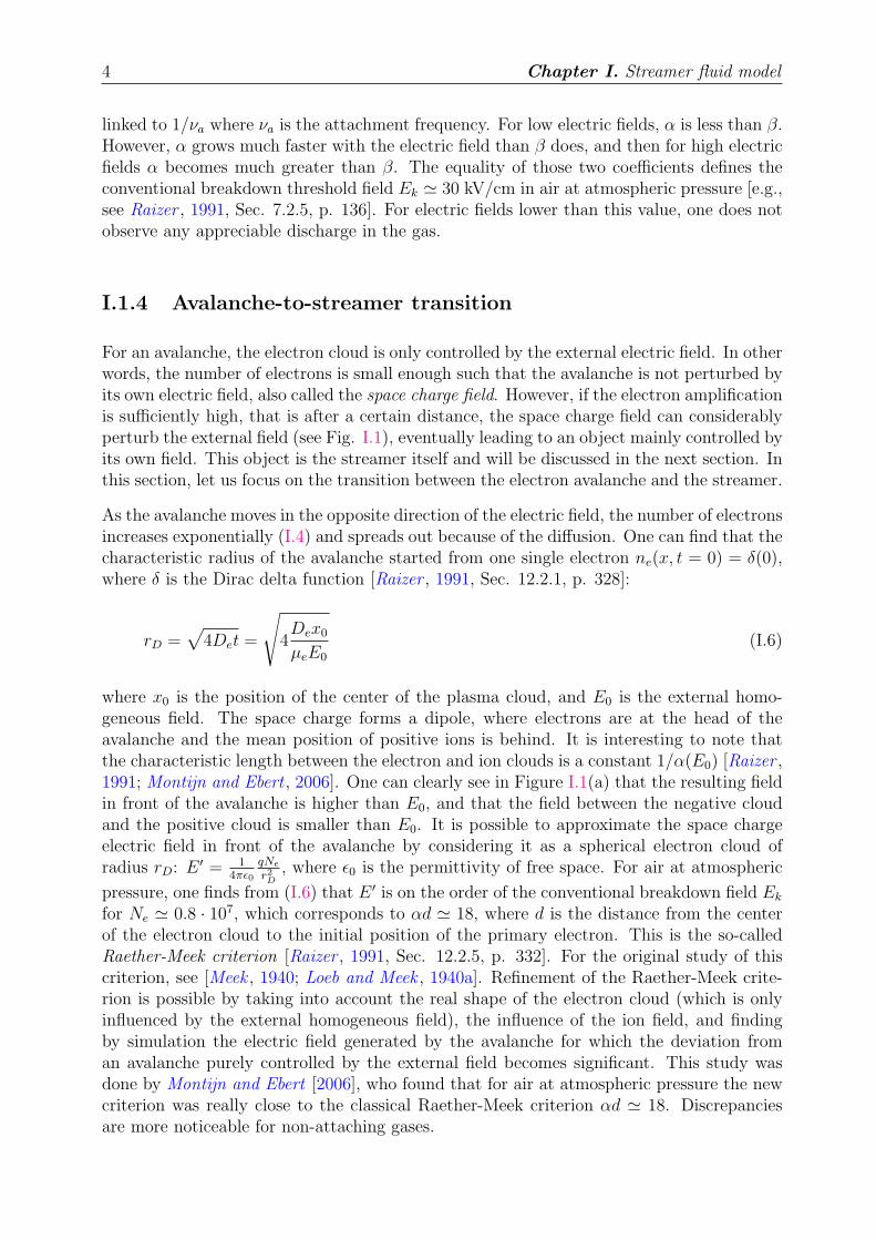
For an avalanche, the electron cloud is only controlled by the external electric field. In otherwords, the number of electrons is small enough such that the avalanche is not perturbed byits own electric field, also called the space charge field. However, if the electron amplificationis sufficiently high, that is after a certain distance, the space charge field can considerablyperturb the external field (see Fig. I.1), eventually leading to an object mainly controlled byits own field. This object is the streamer itself and will be discussed in the next section. Inthis section, let us focus on the transition between the electron avalanche and the streamer.
As the avalanche moves in the opposite direction of the electric field, the number of electronsincreases exponentially (I.4) and spreads out because of the diffusion. One can find that thecharacteristic radius of the avalanche started from one single electron ne(x, t = 0) = δ(0),where δ is the Dirac delta function [Raizer , 1991, Sec. 12.2.1, p. 328]:
rD =√
4Det =
√
4Dex0
µeE0
(I.6)
where x0 is the position of the center of the plasma cloud, and E0 is the external homo-geneous field. The space charge forms a dipole, where electrons are at the head of theavalanche and the mean position of positive ions is behind. It is interesting to note thatthe characteristic length between the electron and ion clouds is a constant 1/α(E0) [Raizer ,1991; Montijn and Ebert , 2006]. One can clearly see in Figure I.1(a) that the resulting fieldin front of the avalanche is higher than E0, and that the field between the negative cloudand the positive cloud is smaller than E0. It is possible to approximate the space chargeelectric field in front of the avalanche by considering it as a spherical electron cloud ofradius rD: E ′ = 1
4πǫ0
qNe
r2D
, where ǫ0 is the permittivity of free space. For air at atmosphericpressure, one finds from (I.6) that E ′ is on the order of the conventional breakdown field Ek
for Ne ≃ 0.8 · 107, which corresponds to αd ≃ 18, where d is the distance from the centerof the electron cloud to the initial position of the primary electron. This is the so-calledRaether-Meek criterion [Raizer , 1991, Sec. 12.2.5, p. 332]. For the original study of thiscriterion, see [Meek , 1940; Loeb and Meek , 1940a]. Refinement of the Raether-Meek crite-rion is possible by taking into account the real shape of the electron cloud (which is onlyinfluenced by the external homogeneous field), the influence of the ion field, and findingby simulation the electric field generated by the avalanche for which the deviation froman avalanche purely controlled by the external field becomes significant. This study wasdone by Montijn and Ebert [2006], who found that for air at atmospheric pressure the newcriterion was really close to the classical Raether-Meek criterion αd ≃ 18. Discrepanciesare more noticeable for non-attaching gases.
I.1. Electron avalanche 5
Figure I.1: Avalanche between two planar electrodes (A is the anode and C is the cathode)generating the homogeneous electric field ~E0. (a) Representation of the space charge electricfield ~E ′. (b) Representation of the total electric field ~E = ~E0 + ~E ′. Figure taken from[Raizer , 1991, Fig. 12. 3, p. 332].
When the density of electrons is sufficiently high in the avalanche head (i.e., when αd & 14),the role of repulsion between electrons becomes non-negligible compared to diffusion for theexpansion of the radius of the avalanche. Furthermore, the rate of expansion due to diffusionis δrD/δt ∼ t−1/2, but the rate of expansion due to the repulsion is given by [Raizer , 1991,Sec. 12.2.6, p. 334]:
dR
dt= µeE
′ =qµeR
−2 exp (αµeE0t)
4πǫ0
(I.7)
Which leads to:
R =
(
3q
4πǫ0αE0
)1/3
exp(αx
3
)
=3E ′
αE0
, ne =3Ne
4πR3=
ǫ0αE0
q(I.8)
Equation (I.8) shows that repulsion of electrons results in an exponential increase of theavalanche radius. Furthermore, we see that the electron density is not changed by thisrepulsion effect.
It is interesting to note here that the time scale linked to this expansion rate is the Maxwelltime, also called the dielectronic relaxation time τm. Indeed, dR
dt∼ R/τm, where:
τm =ǫ0
qneµe
(I.9)
which is quite important in the streamer simulations, as we will see in the following. Wenoticed previously that the mean distance between the ion and the electron clouds is char-acterized by 1/α. When the radius reaches this value, the mean distance between ions andelectrons is small, and the spreading of the electrons begins to slow down. The maximumradius of the avalanche is then ∼1/α. In air at atmospheric pressure this value is roughly0.1 cm at the breakdown field Ek. This phenomenon takes place before the Raether-Meekcriterion is reached, but we see what is taking place for this avalanche: it starts to bemanaged by its own charge field. Afterwards, the Raether-Meek criterion is overtaken, and
6 Chapter I. Streamer fluid model
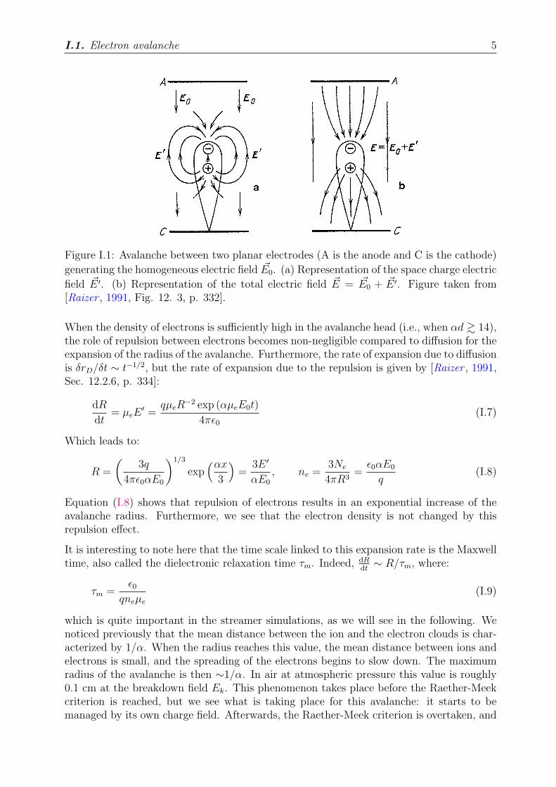
Figure I.2: Diagram of a positive streamer propagating in an ambient field [Liu, 2006;Bazelyan and Raizer , 1998].
the field in front of the avalanche is able to ionize the gas close to this head. This alsooccurs at the back of the avalanche where the ion density is high. These new electronsallow propagation due to drift to be replaced by a new mode based on the ionization of theneutral gas, and this new propagating object is called the streamer discharge.
I.2 Mechanism of streamer discharge propagation
I.2.1 Basics
The concept of streamer discharges was put forward in the 1930’s by Raether and Loeb toexplain spark discharges and by Cravath and Loeb to explain very fast phenomenon (i.e.,close to the speed of light) in low pressure long tubes first observed by J. J. Thompson in1893 [Loeb, 1965]. Meek, Loeb and Raether further developed this theory [Loeb and Meek ,1940a, b; Loeb, 1965].
The concept of streamers is based on a mode of propagation: they are filamentary plasmasdriven by their own space charge field. The dynamics of the streamer is mainly controlledby a high-field region called the streamer head. The head of the streamer is depicted as acrescent shape in the left panel of Figure I.2. In the head the net charge is high and positiveor negative for a positive streamer or negative, respectively. The principle is that the high-field region is quickly enhanced by electrons that drift and amplify on the length scale of thisregion, in a kind of avalanche. In the case of positive streamers, they neutralize the positivecharge zone and therefore the space charge electric field, but repeat the charge pattern abit farther down by leaving the ions behind them during their drift. If the electrons areamplified enough to compensate the positive head of the streamer, then the streamer canpropagate in a stable manner. Thus, the positive streamer propagates step-by-step in thedirection of the ambient field, which is why the streamer is also called a space charge wave.For air at atmospheric pressure, the streamers propagate very fast: typically with velocity∼108 cm/s, that is one hundredth of the speed of light in the vacuum. The peak of electricfield in the streamer head can reach 4-7 times the breakdown field Ek [e.g., see Dhali andWilliams , 1987; Liu, 2006].
Therefore, the positive streamer moves in the reverse direction of the electrons. Then, it
I.2. Mechanism of streamer discharge propagation 7
needs electrons upstream its head to propgate. These electrons may come from the naturalelectron background, essentially due to natural radioactivity and cosmic rays, from a pre-ionization of the gas, for example due to previous discharges or photoionization by externalsource (UV lamps, etc). Furthermore, the high-field region is the place of very intenseelectron impact on neutral molecules which leads to ionization, excitation, or creation ofactive species. The molecules excited by the electron impact can relax to lower energystates by emitting photon radiation. A certain range of photons can themselves ionizeneutral molecules by photoionization, which provide seed electrons ahead of the streamer.These electrons enter the high-field region and participate in its enhancement of electrondensity. The photoionization has been found to be essential for the positive streamers topropagate with the observed velocities. This physical phenomenon and its modeling willbe extensively discussed in Chapter III.
For negative streamers, the principle of propagation is the same but the net charge in thehead is negative and it propagates in the opposite direction of positive streamers, that isin the opposite direction of the electric field. Thus, electrons behind the streamer headparticipate in the local electron amplification in the high-field region. Pre-ionization andphotoionization are then less important in the case of negative streamers. However, as forpositive streamers, pre-ionization level and photoionization play important roles in theirstructures and guide streamer propagation [e.g., Vitello et al., 1994].
For both streamer types, the forward-moving streamer head leaves behind quasi-neutralplasma, where the field is very low (E . Ek). This is often called the streamer channel, orstreamer tail, and can be described as an ambipolar zone [e.g., Hassouni et al., 2004].
I.2.2 Estimation of the propagation velocity
An electron which enters the streamer head ignites the avalanche at a time t, until theelectron density, due to the amplification from this electron, reaches the positive ion densityat a time t + δt. Assuming this amplification behaves like an avalanche for a constantfield, one can estimate that the characteristic distance between the new created electronsneutralizing the streamer head and the new created ions left behind is α−1, as for theclassical avalanche (see previous section). The characteristic length of the streamer headis then δl ∼ α(Emax)
−1, where Emax is the maximum field in the streamer head. Thecharacteristic time of ionization over such a characteristic length is precisely the ionizationtime: δt ∼ νi(Emax)
−1. Then one obtains a rough estimation of the propagation velocity Vs
by writing:
Vs ∼ α(Emax)−1νi(Emax) = ve(Emax) (I.10)
We can find in results provided in [Dhali and Williams , 1987] that this approximation isquite accurate, given the simplicity of this relation. In fact, Vs calculated here is underes-timated by less than one order of magnitude.
A more complete approximation has been derived in [Dyakonov and Kachorovskii , 1988],which presents a clear relation between the propagation velocity and the density far beyondthe streamer head. One can consider that, as for an electrode with a tip radius R, the regionaround the streamer head with a substantial field has a size on the order of the streamerradius R. Moreover, it is well known that the ionization frequency is a function of the
8 Chapter I. Streamer fluid model
electric field and saturates above a field Es. Dyakonov and Kachorovskii [1988] concludedthat the size of the substantial field region (∼R) around the streamer head should be onthe same order as the size of the region where substantial ionization takes place, for thestreamer to have a stable propagation. Then, the field at the streamer head would be on theorder of Es, and then one has νi ∼ νi(Es) ≡ νi,s in this region. The increase of the electrondensity in the high field region stops when the repulsion of electrons is faster than theionization, that is when the Maxwell time is on the order of the ionization time: τm ∼ ν−1
i,s
(see Section I.1.4). For the exponential growth of the electron density n(t) = n0 exp (νi,st),where n0 is the electron density far beyond the streamer head (e.g., due to photoionization),one finds that the characteristic time of the electron density growth is:
τ ∼ ν−1i,s log
(
νi,sǫ0
qn0µe
)
(I.11)
One sees that in these conditions the density in the streamer channel is:
nc ∼ n(t = τ) =νi,sǫ0
qµe
(I.12)
Thus, one obtains the streamer velocity:
Vs ∼R
τ=
Rνi,s
log(nc/n0)(I.13)
As a qualitative result, one sees that the smaller nc/n0 (keeping the other parameters asconstants), the faster the streamer. In [Dyakonov and Kachorovskii , 1989] authors showedthat their model (not restricted to Equation (I.13)) was in good agreement with [Dhali andWilliams , 1987]. Note that a similar equation of the streamer propagation velocity wasalready provided by Loeb [1965], and that two other analytical models are provided in [Ku-likovsky , 1998]. Kulikovsky [2000b] also proposed to replace R in (I.13) by the characteristiclength of the absorption of photoionizing radiation. However, these models all contain atleast one arbitrary parameter which is a priori not known (e.g., n0 in (I.13)).
As for the calculation of the streamer velocity, a full and accurate investigation of thestreamer properties is only possible by a more complete description than the existing an-alytical models, and due to the high non-linearity of the source terms and the transportcoefficients, the numerical simulation is required.
I.3 Model formulation
I.3.1 Elements of kinetic theory
Kinetic theory aims at describing the motion of particles by one distribution functionf(~r,~v, t). The statistical meaning of the number f(~r,~v, t)d3rd3v is the number of par-ticles (electrons in our case) inside the phase-space volume d3rd3v at (~r,~v) and at time t.On this basis one can define the density of particles:
n(~r, t) =
∫
f(~r,~v, t)d3v (I.14)
I.3. Model formulation 9
and the mean velocity of the group of particles, also named the fluid velocity :
~V (~r, t) = 〈~v〉v ≡ 1
n(~r, t)
∫
~vf(~r,~v, t)d3v (I.15)
In the same way, we can obtain the characteristic frequencies of collision from their crosssections, for example:
ν(~r, t) = N〈σ~v〉v =N
n(~r, t)
∫
σ~vf(~r,~v, t)d3v (I.16)
where N is the neutral molecule density and σ is the momentum transfer cross section.
The evolution of the distribution function is governed by the Boltzmann equation:
∂f
∂t+ ~v · ~∇~rf +
~F
m· ~∇~vf =
(
∂f
∂t
)
c
(I.17)
where ~F is the force exerted on the particles and(
∂f∂t
)
caccounts for the change in f due to
collisions.
I.3.2 Fluid reduction
It is possible to obtain a very good description of the dynamics of particles by taking thefirst moments of Equation (I.17). However, the dynamics of moment vk is coupled to thedynamics of moment vk+1. It is then necessary to truncate the moment series at a finitestage. We will take the first two moments of (I.17). The first moment (k = 0) of theelectron Boltzmann equation gives the continuity equation:
∂ne
∂t+ ~∇ · (ne
~Ve) = G − L (I.18)
where subscript “e” stands for “electrons”. The functions G and L describe the creationrate and the loss rate for electrons, respectively. The second moment of the Boltzmannequation gives the conservation of momentum flux, also called the Euler equation:
∂ ~Ve
∂t+ ( ~Ve · ~∇) ~Ve = −
~∇Pe
neme
+〈 ~Fe〉vme
− ν ~Ve (I.19)
for a weakly ionized plasma where only electron-neutral collisions are taken into account.The quantity Pe in (I.19) is the electron pressure.
It is very interesting to see how we can simplify the Euler equation. First, the first termof the left-hand side of Equation (I.19) falls very quickly to zero, since the electron flowvelocity ~Ve we consider here becomes stationnary on a time scale on the order of at mostν−1, which is short compared to the propagation time scale of the streamer:
∂Ve
∂t∼ 0
Second, since the streamer proceeds as a fast ionization wave, one has in principle Vs & Ve.The quantity δl ∼ α−1 is the characteristic length of the flow. Therefore, ν ≃ 3 ·1012 s-1 (see
10 Chapter I. Streamer fluid model
Section I.1.1) is much greater than Ve/δl . Vsα ≃ 109 s-1, for Vs ≃ 108 cm/s and α ≥ 10cm-1 (see previous discussion), and one gets:
νVe =vthVe
λ≫ V 2
e
δl∼ |( ~Ve · ~∇) ~Ve|
where λ is the mean free path of momentum transfer, and vth is the usual thermal velocityof electrons. In fact, one has: V 2
e
δl= V 2
e
λKn, where Kn = λ/δl is called the Knudsen
number and characterizes whether the fluid is in molecular or continuous flow. In our caseλ ≪ δl ⇒ Kn ≪ 1 and therefore the regime is continuous and the inertial term is neglectedcomparing to the friction force [Rax , 2005, Sec. 6.2.1]. Thus, from this short analysis onecan neglect the left-hand side of Equation (I.19) and one obtains:
~Ve = −~∇Pe
meneν+
〈 ~Fe〉vmeν
(I.20)
On time scale of electron flow larger than (δν)−1, one can consider the electrons as a locallyisothermal fluid, and thus assume Pe = nekTe. This leads to the relation for the fluidvelocity:
~Ve = − kTe
meν
~∇ne
ne
+〈 ~Fe〉vmeν
= −De
~∇ne
ne
+ µe〈 ~Fe〉v
q(I.21)
This equation closes the system of moments of the Boltzmann equation. Note that althoughwe focused on the motion of electrons, positive ions can be treated in a similar fashion.
I.3.3 Lorentz force and magnetic field
As the electric field due to the streamer head varies very quickly in the reference frameof the experimentalist, one can ask if the induced magnetic field has a role in governingstreamer propagation in an external constant Laplacian electric field. The magnetic fieldis governed by the Maxwell-Ampère Equation:
~∇× ~B = µ0qne~Ve + µ0ǫ0
∂ ~E
∂t(I.22)
where ~B is the magnetic field, and µ0 is the permeability of free space. Now, let us makean approximate analysis to see under what conditions one can neglect the magnetic field.
We consider the characteristic length scale δl to be on the order of the size of the streamerhead radius. We saw in Section I.2.2 that in the streamer dynamics this length scale canbe linked to the time scale δt ≃ ν−1
i,max log(nc/n0). Thus, one can approximate the terms ofleft and right sides of Equation (I.22) as:
|~∇× ~B| ∼ B
δland µ0qne| ~Ve| + µ0ǫ0
∣
∣
∣
∣
∣
∂ ~E
∂t
∣
∣
∣
∣
∣
∼ qneµeE
ǫ0c2+
1
c2
E
δt
where we used the relation ǫ0µ0c2 = 1, with c being the speed of light in free space. We
therefore obtain the approximation2 for B:
B ∼ qneµeEδl
ǫ0c2+
1
c2
Eδl
δt(I.23)
2Because of the triangle inequality, B is actually overestimated in the Equation (I.23).
I.3. Model formulation 11
We see that the Maxwell time (I.9) appears in Equation (I.23):
B ∼(
1
τm
+1
δt
)
δl
c2E (I.24)
Besides, we saw in Section I.1.4 and I.2.2 that the Maxwell time becomes comparable tothe ionization time τm ∼ ν−1
i,max in the streamer head. The electron density in the streamerchannel is much greater than that ahead of the streamer. Therefore nc/n0 ≫ 1, and even ifthis factor is in the logarithm (log (nc/n0) ≃ 10 typically in our studies), one can considerthat δt−1 ≃ νi,max/ log(nc/n0) is negligible compared to τ−1
m . Moreover, according to (I.13)one has the streamer velocity Vs ∼ δl/δt. Therefore, one obtains:
B ∼ δl
c2τm
E =δl
δt
log (nc/n0)
c2E =
Vs
c2log (nc/n0) (I.25)
The electron fluid is subject to the mean Lorentz force:
〈~F 〉v = q( ~E + ~Ve × ~B) ∼ q ~E + qVeVs
c2log (nc/n0)E~um (I.26)
where ~um =~Ve× ~B
| ~Ve× ~B| . We know that at most, the mean velocity of the electron fluid is Ve . Vs
in the streamer head:
q| ~Ve × ~B| . qV 2
s
c2log (nc/n0)E
And since Vs ≪ c (in air at atmospheric pressure Vs/c ≃ 1/100), one has:
〈~F 〉v ∼ q ~E (I.27)
Thus, the motion of the electron fluid is only subjected to the electrostatic force, and this isthe approximation we will employ in the rest of this work. Note that the streamer model wepresent in Section I.4 does not prevent the streamer velocities from reaching and exceedingthe speed of light [see Liu and Pasko, 2004, Sec. 4.3]. However, the streamers we will studyhave a much lower velocity than light in vacuum.
I.3.4 Diffusion coefficient
The analysis made in section I.3.2 to obtain Equation (I.21) is not general. Indeed, weassumed that the problem was perfectly isotropic and that De was a scalar. Generally,this is not true in the presence of high density gradients and if the collision frequency formomentum transfer depends on electron energy [Parker and Lowke, 1969]. Typically forelectrons, ν increases with energy which leads to a slowing down of these electrons. Inthe presence of high density gradients, the mean energy of electrons going down throughthe gradient in the opposite direction of the field is not compensated by the less numerouselectrons passing in the other direction. These energetic electrons encounter a greaterfriction force due to the increase in collision frequency. On a mesoscopic scale, this behavioris equivalent to a reduction of the coefficient of diffusion in the direction of the field D‖compared to that of diffusion in the transverse direction D⊥. At most, D‖ and D⊥ differ bya factor of 2 [Raizer , 1991, Sec 2.4.4, p. 23]. In the streamers we study here, the gradientsof electron density are not high enough for electron diffusion to significantly affect thestreamer dynamics, which is principally governed by the electron drift and source terms.Thus, these differences in the diffusion coefficients are considered to be negligible, and wetake D‖ = D⊥ = De.
12 Chapter I. Streamer fluid model
I.3.5 Local field approximation
As is very often the case in the literature, we will assume that the local field approxima-tion is valid in our study. This approximation implies that local equilibrium of electrons isachieved instantaneously in time in response to the electric field ~E. This allows us to expressall the transport coefficients and source terms as explicit functions of the norm of the localreduced electric field E/N . This is the case when the time scales of variations of the electricfield and electron density are long compared to the time scale of energy relaxation, and thisapproximation is not always valid in the streamer head. Several approaches have been takento examine the differences due to the nonlocality in streamers. The first one consists of tak-ing nonequilibrium into account by adding additional moments of the Boltzmann equationto increase the accuracy of the fluid description [Kunhardt et al., 1988]. In [Guo and Wu,1993] an equation of the energy balance appears naturally, and therefore the mean energyof electrons is used in the ionization coefficient as part of streamer simulations (positiveand negative) for nitrogen at atmospheric pressure. The effects of nonlocality on positivestreamers in air at atmospheric pressure were studied by Naidis [1997], who corrected theelectron source term rates calculated with the local field approximation following the workof [Aleksandrov and Kochetov , 1996]. Deviations from the local field approximation werestudied for negative streamers in nitrogen at atmospheric pressure by [Li et al., 2007] bymeans of a comparison between 1D fluid and particle models. By taking into account thenonlocal effects, all of these authors found an increase of the ionization in the streamerhead, a resulting increase of the electric field and a small increase of the streamer velocity.
However, these discrepancies are far smaller than an order of magnitude. For example,Li et al. [2007] found a relative difference between the fluid and the particle models of∼10% and ∼20% in the ionization level behind the streamer front for homogeneous appliedelectric fields of 50 kV/cm and 100 kV/cm, respectively. For practical accuracy, one canobtain the main streamer characteristics by a fluid model [Naidis , 1997]. Furthermore,recently Chanrion and Neubert [2008] used a PIC code to solve the Boltzmann equation anda Monte Carlo simulation to simulate collisions, in the framework of streamer simulationsin the Earth’s atmosphere as applicable to sprite discharges. These authors found anexcellent agreement with results obtained by a fluid model by Liu and Pasko [2004] (acomparison of our results with this work will be presented in Chapter III) both for positiveand negative streamers. This agreement is surprisingly good, as noted by the authorsthemselves, especially given the discrepancies in the modeling of the photoionization and ofcourse in the local field approximation used in [Liu and Pasko, 2004] but not in [Chanrionand Neubert , 2008]. We will thus also assume that the local field approximation is valid inthe following section.
I.4 Streamer equations
From the previous sections of this chapter, one can derive the most common and effectivemodel to study the dynamics of streamers based on the following drift-diffusion equationsfor electrons and ions coupled with Poisson’s equation [e.g., Kulikovsky , 1997b]:
∂ne
∂t+ ~∇·(ne ~ve) − ~∇ · (De
~∇ne) = Sph + S+e − S−
e (I.28)
I.4. Streamer equations 13
∂np
∂t+ ~∇·(np ~vp) = Sph + S+
p − S−p (I.29)
∂nn
∂t+ ~∇·(nn ~vn) = S+
n − S−n (I.30)
~∇2V = − q
ǫ0
(np − nn − ne) (I.31)
where subscripts “e”, “p” and “n”, respectively, refer to electrons, positive and negativeions, ni is the number density of species i, V is the potential, ~ve is the drift velocity ofelectrons, Di and µi are respectively the diffusion coefficient and the absolute value ofmobility of species i, q is the absolute value of electron charge, and ǫ0 is permittivity offree space. The S+ and S− terms stand for the rates of production and loss of chargedparticles. They will be taken with the following general form:
S+e = S+
p = neαve (I.32)
S+n = neβattve (I.33)
S−e = neβattve + nenpβep (I.34)
S−p = nenpβep + nnnpβnp (I.35)
S−n = nnnpβnp (I.36)
where βatt accounts for the electron attachment on neutral molecules, βep accounts for theelectron-positive ion recombination, and βnp accounts for the negative-positive ion recom-bination. In the present study, the S+
e and S+p production rates are the ionization rate due
to the electron impact ionization of air molecules. The origin of the coefficient sets we usewill be indicated each time, as needed.
The Sph term is the rate of electron-ion pair production due to photoionization in a gasvolume. For photoionization calculations in the streamer model, we employed techniquesdiscussed in Chapter III. Specifically, for the present study we have implemented the three-group Eddington and SP3, the three-exponential Helmholtz, and the Zheleznyak classicalintegral models [Ségur et al., 2006; Bourdon et al., 2007; Zheleznyak et al., 1982].
The coefficients of the model are assumed to be explicit functions of the local reducedelectric field E/N , where E is the electric field magnitude and N is the neutral density ofair (see Section I.3.5).
As a rough approximation, one can consider that the characteristic length of the variationof electron and ion densities in the streamer head is on the order of α−1 (see Section I.2.2).One notes ~vdiffi
= −Di~∇ni/ni the “diffusion velocity” of ions (positive or negative). Using
the Einstein relation (I.3) it then follows that vdiffi/vi = Di|~∇ni|/(nivi) ∼ Diα/(µiEmax) =
kTiα/(qEmax) ≃ 10−2, since the ion temperature is roughly the ambient temperature, usingEmax ≃ 150 kV/cm and by taking α from [Morrow and Lowke, 1997] (e.g., see Section II.3).The density gradients are even weaker in the streamer channel and before the streamer head.Thus, in all cases we present in this Ph.D. thesis, the diffusion of ions will be neglected. Asimilar analysis for an electron thermal energy of ∼1 eV shows that the electron diffusionis mostly negligible compared to the drift velocity of the electrons.

14 Chapter I. Streamer fluid model
In this report, axisymmetric streamers are studied and thus cylindrical coordinates areused.
The computational models used for solving the drift-diffusion equations as well as for Pois-son’s equation are described in Chapter II.

Chapter II
Numerical models
Table of ContentsII.1 Poisson’s equation . . . . . . . . . . . . . . . . . . . . . . . . . . . 16
II.1.1 Discretization . . . . . . . . . . . . . . . . . . . . . . . . . . . . . 16
II.1.2 Boundary conditions . . . . . . . . . . . . . . . . . . . . . . . . . 17
External homogeneous electric field . . . . . . . . . . . . . . . . . 18
Field generated by a spherical electrode placed in an weak externalhomogeneous electric field . . . . . . . . . . . . . . . . . 19
Elliptic integral approach . . . . . . . . . . . . . . . . . . . . . . 20
II.1.3 Numerical methods for solving Poisson’s equation . . . . . . . . . 21
II.2 Numerical resolution of the drift-diffusion equations . . . . . . 23
II.2.1 Finite volume methods . . . . . . . . . . . . . . . . . . . . . . . . 23
II.2.2 Numerical schemes for drift-diffusion fluxes . . . . . . . . . . . . 27
Upwind scheme for drift fluxes . . . . . . . . . . . . . . . . . . . 27
Flux Corrected Transport method . . . . . . . . . . . . . . . . . 27
Modified Scharfetter-Gummel scheme . . . . . . . . . . . . . . . 28
Diffusion fluxes . . . . . . . . . . . . . . . . . . . . . . . . . . . . 30
II.2.3 Time integration . . . . . . . . . . . . . . . . . . . . . . . . . . . 30
Time step . . . . . . . . . . . . . . . . . . . . . . . . . . . . . . . 30
II.3 Numerical results . . . . . . . . . . . . . . . . . . . . . . . . . . . 31
II.4 Conclusions . . . . . . . . . . . . . . . . . . . . . . . . . . . . . . . 37
16 Chapter II. Numerical models
II.1 Poisson’s equation
For streamer simulations, the electric field is a key parameter for two reasons. First, thetransport parameters and source terms have a non-linear dependence on it. Second, the
electric field is directly related to charged species densities (I.31). In streamer simulations,the electric field is derived from the electric potential given by Poisson’s equation. A smallerror in the calculation of the electric potential leads to large fluctuations in the electricfield, which may lead to considerable errors in the simulation results. Thus, it is importantto solve Poisson’s equation accurately. Moreover, we show in Chapter III that techniquessimilar to those we use for solution of Poisson’s equation are also used for the modeling ofthe photoionization source term.
Three important points have to be considered for the numerical solution of Poisson’s equa-tion:
• The discretization scheme: it defines the numerical accuracy of the resolution ofPoisson’s equation. The discretization we use is derived in Section II.1.1.
• The boundary conditions: as an elliptic equation, the resolution of Poisson’s equationrequires the boundary conditions to be set. It is especially important in the case ofLaplace’s equation where the solution is entirely governed by the boundary conditions.We discuss this point in Section II.1.2, and we present in detail the calculation ofboundary conditions for two configurations studied in this work.
• The numerical method used: the resolution of Poisson’s equation can be very timeconsuming. For this reason, one has to find the most efficient solver for each newconfiguration under study. Some solvers are iterative, and some are direct. In thepresent work, both are used and we will briefly present them and compare them inSection II.1.3.
II.1.1 Discretization
In cylindrical coordinates, Equation (I.31) can be written as:
∂
∂x
(
∂V
∂x
)
+1
r
∂
∂r
(
r∂V
∂r
)
= −ρ(x, r)
ǫ0
(II.1)
where x and r are axial and radial coordinates, respectively, and ρ = q(np−nn−ne). In thiswork, we consider that the computational domain is discretized on a rectilinear grid. Thenodes of the grid are indexed with i and j in the axial and radial directions respectively,
II.1. Poisson’s equation 17
such that Vi,j = V (xi, rj). The edges of the cell indexed (i, j) are located by xi±1/2 andrj±1/2, in the axial and radial direction, respectively (see Figure II.6).
In the volume of the computational domain (i.e., far from the boundaries) the second orderdiscretization of Eq. (II.1) in cylindrical coordinates gives the classical five diagonal linearsystem:
V ei,jVi+1,j + V w
i,jVi−1,j + V si,jVi,j−1 + V n
i,jVi,j+1 + V ci,jVi,j = −ρi,j
ǫ0
(II.2)
with:
V ei,j =
1
∆xi(xi+1/2 − xi−1/2)
V wi,j =
1
∆xi−1(xi+1/2 − xi−1/2)
V ni,j =
rj+1/2
∆rj
(
r2j+1/2
−r2j−1/2
2
)
V si,j =
rj−1/2
∆rj−1
(
r2j+1/2
−r2j−1/2
2
)
V ci,j = −(V w
i,j + V ei,j + V s
i,j + V ni,j)
(II.3)
where ∆xi = xi+1 − xi and ∆rj = rj+1 − rj. In this work, we have used this second orderdiscretization of Poisson’s equation because it is sufficiently accurate and robust for thecases we have considered.
II.1.2 Boundary conditions
Different sets of boundary conditions are used for Poisson’s equation, depending on theproblem studied. In this work, we have considered discharges propagating between twoelectrodes (plane-to-plane, point-to-plane and point-to-point). For metallic electrodes, thepotential is fixed on the electrodes, and in Chapter IV we will present how to impose thisboundary condition for an electrode of complex shape in a rectilinear mesh. The caseof boundary conditions in presence of a dielectric material will be addressed in ChapterVI. In this work, we have only considered axisymmetric geometries, and thus a symmetrycondition is used on the axis of symmetry.
In this section, we present the calculation of boundary conditions for two different casesthat we have extensively studied for streamer simulations. In the first one, shown in FigureII.1, a strong homogeneous electric field (i.e., greater than Ek everywhere in the simulationdomain) is applied externaly. In order to simulate streamer propagation in a weak electricfield (i.e., less than Ek), the second case shown in Figure II.2 consists of a narrow high-fieldregion generated by a spherical electrode placed in a weak and originally homogeneouselectric field. In this test case the spherical electrode is considered to be outside of thesimulation domain.
18 Chapter II. Numerical models
In streamer simulations, computational domains are usually large in the radial directionsand therefore, the electric potential at the boundary r = R is specified by neglectingcontributions from the charges inside the domain since they occupy a relatively small space.Two different types of boundary conditions can be used at the boundary r = R. Thehomogeneous Neumann boundary condition (~∇V · ~n = 0, ~n being the normal vector of thesurface boundary), and the Dirichlet boundary condition based on the solution of Laplace’sequation (i.e., ρ = 0 in Equations (I.31) and (II.1)).
If one wants to use a computational domain with a smaller radial extension, the influenceof charges inside the domain has to be considered. In this case, It is possible to computedirectly the Dirichlet boundary conditions from a Laplacian potential and to add the influ-ence of the charges on the boundaries from the integral solution of Equation (II.1). Thisapproach is very time-consuming as each node of the boundary requires an integration ofthe charge densities over the whole simulation domain. Therefore, we have carried out sometests to try to find a compromise on the size of the computational domain between:
• a computational domain with a large radial extension, for which the resolution ofequations in the volume of the computational domain (e.g., drift-diffusion equations)is very time consuming,
• a computational domain with a small radial extension, for which the computation ofboundary conditions for Poisson’s equation is very time consuming.
We have observed that the least time-consuming way for a given accuracy and for config-urations presented in this Chapter is to work with a computational domain with a smallradial extension and the integral solution of Poisson’s equation for boundary conditions.We present the detailed calculation of these boundary conditions for the cases presented inFigures II.1 and II.2.
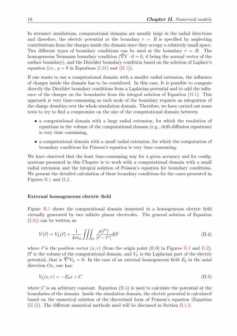
External homogeneous electric field
Figure II.1 shows the computational domain immersed in a homogeneous electric fieldvirtually generated by two infinite planar electrodes. The general solution of Equation(I.31) can be written as:
V (~r) = VL(~r) +1
4πǫ0
∫∫∫
Ω′
ρ(~r ′)
|~r − ~r ′|dΩ′ (II.4)
where ~r is the position vector (x, r) (from the origin point (0, 0) in Figures II.1 and II.2),Ω′ is the volume of the computational domain, and VL is the Laplacian part of the electricpotential, that is ~∇2VL = 0. In the case of an external homogeneous field E0 in the axialdirection Ox, one has:
VL(x, r) = −E0x + C (II.5)
where C is an arbitrary constant. Equation (II.4) is used to calculate the potential at theboundaries of the domain. Inside the simulation domain, the electric potential is calculatedbased on the numerical solution of the discretized form of Poisson’s equation (Equation(II.2)). The different numerical methods used will be discussed in Section II.1.3.
II.1. Poisson’s equation 19
Figure II.1: Representation of the simulation domain in a homogeneous electric field gen-erated by two infinite planar electrodes [Liu and Pasko, 2004].
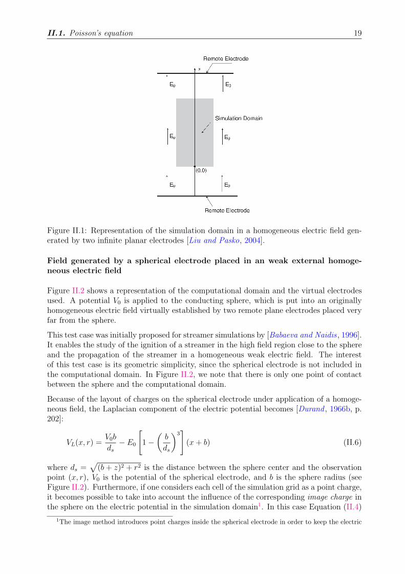
Field generated by a spherical electrode placed in an weak external homoge-neous electric field
Figure II.2 shows a representation of the computational domain and the virtual electrodesused. A potential V0 is applied to the conducting sphere, which is put into an originallyhomogeneous electric field virtually established by two remote plane electrodes placed veryfar from the sphere.
This test case was initially proposed for streamer simulations by [Babaeva and Naidis , 1996].It enables the study of the ignition of a streamer in the high field region close to the sphereand the propagation of the streamer in a homogeneous weak electric field. The interestof this test case is its geometric simplicity, since the spherical electrode is not included inthe computational domain. In Figure II.2, we note that there is only one point of contactbetween the sphere and the computational domain.
Because of the layout of charges on the spherical electrode under application of a homoge-neous field, the Laplacian component of the electric potential becomes [Durand , 1966b, p.202]:
VL(x, r) =V0b
ds
− E0
[
1 −(
b
ds
)3]
(x + b) (II.6)
where ds =√
(b + z)2 + r2 is the distance between the sphere center and the observationpoint (x, r), V0 is the potential of the spherical electrode, and b is the sphere radius (seeFigure II.2). Furthermore, if one considers each cell of the simulation grid as a point charge,it becomes possible to take into account the influence of the corresponding image charge inthe sphere on the electric potential in the simulation domain1. In this case Equation (II.4)
1The image method introduces point charges inside the spherical electrode in order to keep the electric
20 Chapter II. Numerical models
Figure II.2: Representation of the simulation domain where the electrical field is generatedby a spherical electrode in a homogeneous electric field [Liu and Pasko, 2006].
becomes:
V (~r) = VL(~r) +1
4πǫ0
∫∫∫
Ω′
ρ(~r ′)
|~r − ~r ′|dΩ′ +1
4πǫ0
∫∫∫
Ω′
ρi(ρ(~r ′))
|~r − ~ri(~r ′)|dΩ′ (II.7)
where VL(~r) is defined by Equation (II.6) and ρi is a virtual charge density accounting forthe influence of the image charges. One has [Durand , 1966b; Liu, 2006]:
ρi(ρ(~r ′)) = − b
ds
ρ(~r ′) (II.8)
~ri(~r′) =
b2
d2s
(~r ′ + b ~ux) − b ~ux (II.9)
where ~ux is the unit vector of the x-axis. As for Equation (II.4), the integrals in Equation(II.7) are only computed on the boundaries of the simulation domain.
Elliptic integral approach
The calculation of the integrals in Equations (II.4) and (II.7) is very time-consuming.Therefore, we have carried out some tests to compare different numerical methods for com-puting them, namely, by Gaussian quadrature, Romberg’s method and an elliptic integralapproach [these methods were taken from Press et al., 1992]. For studies presented in thiswork, the most efficient numerical method is the elliptic integral approach [Liu and Pasko,2006].
potential as a constant V0 on its surface.
II.1. Poisson’s equation 21
As the model is cylindrically symmetric, one can integrate over the volume of the simula-tion domain using elementary rings of radius r′ at axial position x′, corresponding to anindividual grid node, around the axis of symmetry. Thus, the elementary potential at theobservation point ~r due to this infinitesimal ring is:
dV (x, r; x′, r′) =1
4πǫ0
ρ(x′, r′)r′dr′dx′∫ 2π
0
dφ√
r2 + r′2 + (x − x′)2 − 2rr′ cos φ(II.10)
where φ is the azimuthal angle (see Fig. III.1(a)). By making the substitution φ = π + 2β,one obtains:
dV (x, r; x′, r′) =ρ(x′, r′)r′dr′dx′
πǫ0
√
(r + r′)2 + (x − x′)2K(k(x, r; x′, r′)) (II.11)
where K(k) =∫ 2π
0(1 − k2 sin2 β)1/2dβ is the complete elliptic integral of the first kind, and
k(x, r; x′, r′) = 4rr′
(r+r′)2+(x−x′)2. Note that the denominator in Equation (II.11) is always non-
zero, since we used a simulation grid with cell interfaces at r = 0 or z = 0 instead of gridnodes (see Section II.2.1).
The above method can also be applied to the image part of Equation (II.7). The numericalmethod we used to compute K(k) is taken from [Press et al., 1992] and based on theCarlson’s function RF [Carlson, 1977]. The integration over x′ and r′ is performed usingthe trapezoidal integration.
II.1.3 Numerical methods for solving Poisson’s equation
In streamer simulations, the discretized form of Poisson’s equation (II.2) inside the com-putational domain is usually solved using the symmetrical successive overrelaxation (SOR)method. This method has been widely used because it is simple to implement and ro-bust. However, the SOR method is well-known to converge rather slowly. To reducecomputation times, we have used the D03EBF module of the NAG Fortran library (http:
//www.nag.co.uk) in this work, which is based on the iterative Strongly Implicit Procedure[Stone, 1968]. This method converges more rapidly than the SOR method for the sameaccuracy.
Recently, different efficient direct solvers (e.g., MUMPS [Amestoy et al., 2000, 2001, 2006]and the SuperLU solver [Demmel et al., 1999a, b] (http://crd.lbl.gov/~xiaoye/SuperLU/))have been developed for large systems of linear equations and can be applied to solve Pois-son’s equation. As part of the preparatory work for the studies presented in this thesis,we have conducted several test runs to compare the results obtained using the iterativeNAG module and the direct SuperLU solver. Both solvers have very good performances.The main asset of SuperLU is its accuracy, but its main drawback is the consumption ofmemory and the speed of the LU factorization. On the other hand, the main asset of theNAG routine is that, as an iterative solver, it is faster to converge from previous solutionsthan through a direct matrix inversion, even when using a moving mesh. However, its maindrawback is that it takes a few iterations to converge at each timestep, and moreover, itis difficult to estimate a priori its accuracy for a given set of convergence criteria in eachstudied configuration.
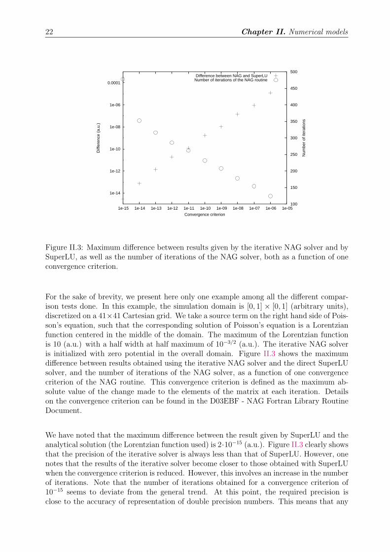
22 Chapter II. Numerical models
1e-14
1e-12
1e-10
1e-08
1e-06
0.0001
1e-15 1e-14 1e-13 1e-12 1e-11 1e-10 1e-09 1e-08 1e-07 1e-06 1e-05 100
150
200
250
300
350
400
450
500
Diff
eren
ce (
a.u.
)
Num
ber
of it
erat
ions
Convergence criterion
Difference between NAG and SuperLUNumber of iterations of the NAG routine
Figure II.3: Maximum difference between results given by the iterative NAG solver and bySuperLU, as well as the number of iterations of the NAG solver, both as a function of oneconvergence criterion.
For the sake of brevity, we present here only one example among all the different compar-ison tests done. In this example, the simulation domain is [0, 1] × [0, 1] (arbitrary units),discretized on a 41×41 Cartesian grid. We take a source term on the right hand side of Pois-son’s equation, such that the corresponding solution of Poisson’s equation is a Lorentzianfunction centered in the middle of the domain. The maximum of the Lorentzian functionis 10 (a.u.) with a half width at half maximum of 10−3/2 (a.u.). The iterative NAG solveris initialized with zero potential in the overall domain. Figure II.3 shows the maximumdifference between results obtained using the iterative NAG solver and the direct SuperLUsolver, and the number of iterations of the NAG solver, as a function of one convergencecriterion of the NAG routine. This convergence criterion is defined as the maximum ab-solute value of the change made to the elements of the matrix at each iteration. Detailson the convergence criterion can be found in the D03EBF - NAG Fortran Library RoutineDocument.
We have noted that the maximum difference between the result given by SuperLU and theanalytical solution (the Lorentzian function used) is 2·10−15 (a.u.). Figure II.3 clearly showsthat the precision of the iterative solver is always less than that of SuperLU. However, onenotes that the results of the iterative solver become closer to those obtained with SuperLUwhen the convergence criterion is reduced. However, this involves an increase in the numberof iterations. Note that the number of iterations obtained for a convergence criterion of10−15 seems to deviate from the general trend. At this point, the required precision isclose to the accuracy of representation of double precision numbers. This means that any
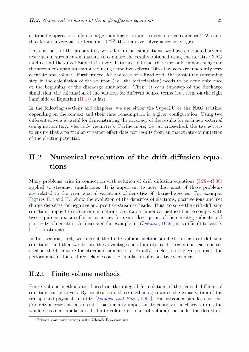
II.2. Numerical resolution of the drift-diffusion equations 23
arithmetic operation suffers a large rounding error and causes poor convergence2. We notethat for a convergence criterion of 10−16, the iterative solver never converges.
Thus, as part of the preparatory work for further simulations, we have conducted severaltest runs in streamer simulations to compare the results obtained using the iterative NAGmodule and the direct SuperLU solver. It turned out that there are only minor changes inthe streamer dynamics computed using these two solvers. Direct solvers are inherently veryaccurate and robust. Furthermore, for the case of a fixed grid, the most time-consumingstep in the calculation of the solution (i.e., the factorization) needs to be done only onceat the beginning of the discharge simulation. Then, at each timestep of the dischargesimulation, the calculation of the solution for different source terms (i.e., term on the righthand side of Equation (II.1)) is fast.
In the following sections and chapters, we use either the SuperLU or the NAG routine,depending on the context and their time consumption in a given configuration. Using twodifferent solvers is useful for demonstrating the accuracy of the results for each new externalconfiguration (e.g., electrode geometry). Furthermore, we can cross-check the two solversto ensure that a particular streamer effect does not results from an inaccurate computationof the electric potential.
II.2 Numerical resolution of the drift-diffusion equa-tions
Many problems arise in connection with solution of drift-diffusion equations (I.28)–(I.30)applied to streamer simulations. It is important to note that most of these problemsare related to the great spatial variations of densities of charged species. For example,Figures II.4 and II.5 show the evolution of the densities of electrons, positive ions and netcharge densities for negative and positive streamer heads. Thus, to solve the drift-diffusionequations applied to streamer simulations, a suitable numerical method has to comply withtwo requirements: a sufficient accuracy for exact description of the density gradients andpositivity of densities. As discussed for example in [Godunov , 1959], it is difficult to satisfyboth constraints.
In this section, first, we present the finite volume method applied to the drift-diffusionequations, and then we discuss the advantages and limitations of three numerical schemesused in the literature for streamer simulations. Finally, in Section II.3 we compare theperformance of these three schemes on the simulation of a positive streamer.
II.2.1 Finite volume methods
Finite volume methods are based on the integral formulation of the partial differentialequations to be solved. By construction, these methods guarantee the conservation of thetransported physical quantity [Ferziger and Peric, 2002]. For streamer simulations, thisproperty is essential because it is particularly important to conserve the charge during thewhole streamer simulation. In finite volume (or control volume) methods, the domain is
2Private communications with Zdenek Bonaventura.
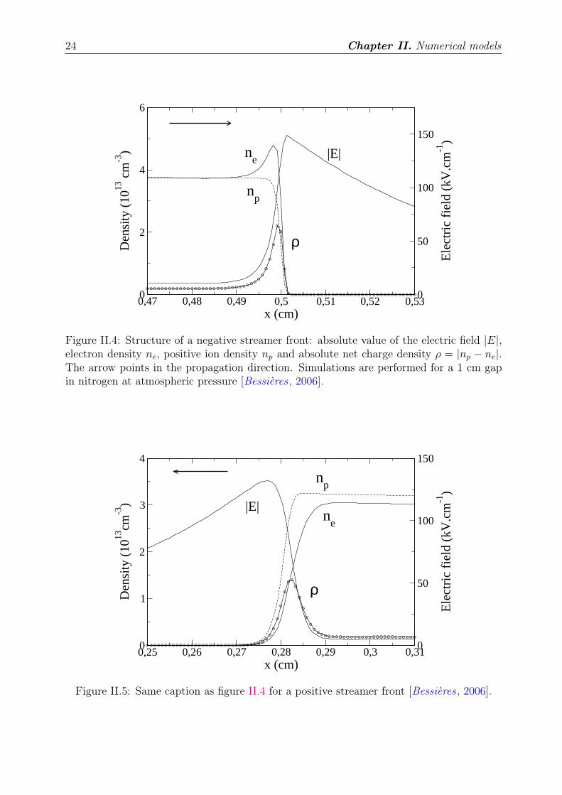
24 Chapter II. Numerical models
0,47 0,48 0,49 0,5 0,51 0,52 0,53x (cm)
0
2
4
6
Den
sity
(10
13 c
m-3
)
0
50
100
150
Ele
ctri
c fi
eld
(kV
.cm
-1)
|E|
np
ρ
ne
Figure II.4: Structure of a negative streamer front: absolute value of the electric field |E|,electron density ne, positive ion density np and absolute net charge density ρ = |np − ne|.The arrow points in the propagation direction. Simulations are performed for a 1 cm gapin nitrogen at atmospheric pressure [Bessières , 2006].
0,25 0,26 0,27 0,28 0,29 0,3 0,31x (cm)
0
1
2
3
4
Den
sity
(10
13cm
-3)
0
50
100
150E
lect
ric
fiel
d (k
V.c
m-1
)
ρ
ne
np
|E|
Figure II.5: Same caption as figure II.4 for a positive streamer front [Bessières , 2006].
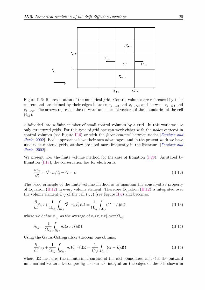
II.2. Numerical resolution of the drift-diffusion equations 25
Figure II.6: Representation of the numerical grid. Control volumes are referenced by theircenters and are defined by their edges between xi−1/2 and xi+1/2, and between rj−1/2 andrj+1/2. The arrows represent the outward unit normal vectors of the boundaries of the cell(i, j).
subdivided into a finite number of small control volumes by a grid. In this work we useonly structured grids. For this type of grid one can work either with the nodes centered incontrol volumes (see Figure II.6) or with the faces centered between nodes [Ferziger andPeric, 2002]. Both approaches have their own advantages, and in the present work we haveused node-centered grids, as they are used more frequently in the literature [Ferziger andPeric, 2002].
We present now the finite volume method for the case of Equation (I.28). As stated byEquation (I.18), the conservation law for electron is:
∂ne
∂t+ ~∇ · ne
~Ve = G − L (II.12)
The basic principle of the finite volume method is to maintain the conservative propertyof Equation (II.12) in every volume element. Therefore Equation (II.12) is integrated overthe volume element Ωi,j of the cell (i, j) (see Figure II.6) and becomes:
∂
∂tni,j +
1
Ωi,j
∫
Ωi,j
~∇ · ne~Ve dΩ =
1
Ωi,j
∫
Ωi,j
(G − L)dΩ (II.13)
where we define ni,j as the average of ne(x, r, t) over Ωi,j:
ni,j =1
Ωi,j
∫
Ωi,j
ne(x, r, t)dΩ (II.14)
Using the Gauss-Ostrogradsky theorem one obtains:
∂
∂tni,j +
1
Ωi,j
∫
∂Ωi,j
ne~Ve · ~n dΣ =
1
Ωi,j
∫
Ωi,j
(G − L)dΩ (II.15)
where dΣ measures the infinitesimal surface of the cell boundaries, and ~n is the outwardunit normal vector. Decomposing the surface integral on the edges of the cell shown in
26 Chapter II. Numerical models
Figure II.6, one obtains:
∂
∂tni,j +
1
Ωi,j
(F xi+1/2 + F x
i−1/2 + F rj+1/2 + F r
j−1/2) = Si,j (II.16)
where we define the fluxes as
F xi+1/2 =
∫
Σi+1/2,j
ne~Ve · ~ndΣ ≃ ni+1/2,jV
xei+1/2,j
Σi+1/2,j (II.17)
where the surface of the cell boundary Σi+1/2,j is located at (i + 1/2, j), and Si,j is theaverage of source and loss terms over the volume Ωi,j.
To calculate the exact change of the density ni,j over an elementary time step ∆t = tk+1−tk,we integrate the equation (II.16) from tk to tk+1:
nk+1i,j = nk
i,j −1
Ωi,j
∫ tk+1
tk(F x
i+1/2 + F xi−1/2 + F r
j+1/2 + F rj+1/2)dt +
∫ tk+1
tkSi,jdt (II.18)
where nk+1i,j is the value of the mean density inside the control volume Ωi,j at the end of
a time step. This equation is the conservative form of Equation (II.16). Indeed, if all thefluxes are equal to zero in a control volume, Equation (II.18) shows that the change ofdensity inside the control volume is only due to volume source and loss terms.
It is important to note that no approximation has been made in deriving Equation (II.18).In order to solve this equation numerically, it is necessary to express the different fluxesand source terms on the right-hand side part of the equation. It is interesting to point outthat the fluxes in Equation (II.18) account for both drift and diffusion fluxes. We will firstconsider the fluxes are constant during time step ∆t and simplify Equation (II.18):
nk+1i,j = nk
i,j −∆t
Ωi,j
(F x,ki+1/2 + F x,k
i−1/2 + F r,kj+1/2 + F r,k
j+1/2) +
∫ tk+1
tkSi,jdt (II.19)
The main problem in solving Equation (II.19) concerns the determination of fluxes at theinterfaces of the control volume. Indeed, as shown by Equation (II.17), these fluxes onlystrictly depend on the (unknown) values of the densities at the interfaces and not on the(known) mean value of the density ni,j inside the control volume. Thus, the difficulty is toexpress the different fluxes as approximate functions of ni,j. In the following section, wewill present the approximate expressions of drift fluxes for the three different schemes usedin this work:
• The upwind scheme.
• A Flux-Corrected Transport method.
• The modified Scharfetter-Gummel scheme.
It is interesting to note that diffusion fluxes are calculated simultaneously with drift fluxesin the modified Scharfetter-Gummel scheme. For other schemes, diffusion and drift fluxesare calculated separately, and we present the method used to calculate diffusion fluxes inthese cases. Finally, in the following section, we will present and discuss different methodsfor the time integration and the integration of the source term on the right-hand side ofEquation (II.16).
II.2. Numerical resolution of the drift-diffusion equations 27
II.2.2 Numerical schemes for drift-diffusion fluxes
In this section, the source term in Equation (II.19) is assumed to be equal to zero:
nk+1i,j = nk
i,j −∆t
Ωi,j
(F x,ki+1/2 + F x,k
i−1/2 + F r,kj+1/2 + F r,k
j+1/2) (II.20)
In cylindrical coordinates, the volumes Ωi,j and the surfaces Σi+1/2,j and Σi,j+1/2 are givenby:
Σi+1/2,j = π(r2i,j+1/2 − r2
i,j−1/2) (II.21)
Σi,j+1/2 = 2πri,j+1/2(zi+1/2,j − zi−1/2,j) (II.22)
Ωi,j = π(r2i,j+1/2 − r2
i,j−1/2)(zi+1/2,j − zi−1/2,j) (II.23)
Upwind scheme for drift fluxes
The upwind scheme is the simplest numerical scheme. The basic idea of this scheme is touse the direction of the drift velocity to approximate the drift fluxes. The drift velocityfield for charged particles can be easily derived at each time step from the calculation of theelectric field. Then, for example in the axial direction, the drift fluxes are approximated as:
• F x,ki+1/2 = nk
i,jvx,kei+1/2,j
Σi+1/2,j, if ~vkei+1/2,j
· ~ni > 0,
• F x,ki+1/2 = −nk
i+1,jvx,kei+1/2,j
Σi+1/2,j, if ~vkei+1/2,j
· ~ni < 0.
where vx,ke is the axial component of the drift velocity ~ve. A similar approximation is used in
the radial direction.The upwind scheme is therefore very simple to implement and has thegreat advantage of being strictly positive. However, this first-order scheme is numericallydiffusive [e.g., Ferziger and Peric, 2002].
This scheme has been used for streamer simulations, in particular in the work of the MIPTgroup in Russia [e.g., Pancheshnyi et al., 2001, 2005].
Flux Corrected Transport method
To reduce the numerical diffusion and thereby increase the accuracy of the solution, differenthigh order interpolation methods can be used to determine the drift fluxes at the cellinterfaces. However, solutions by schemes of second order and higher, are not positive andthese schemes generally present dispersion with spurious oscillations close to high gradientzones [e.g., Ferziger and Peric, 2002]. Different types of methods have been developed in theliterature to reduce the spurious oscillations as much as possible and guarantee the positivityof the solution. The method of Flux Corrected Transport was developed in the 1970s [Borisand Book , 1973, 1976]. The basic idea of this method is to combine two numerical schemes.The first is strictly positive but diffusive (for example the upwind scheme), and the second
28 Chapter II. Numerical models
is a higher order, but dispersive scheme which is more accurate. In the FCT method, thesolution obtained with the low-order diffusive scheme is corrected by antidiffusive fluxescalculated using the high-order scheme. However, as this scheme is dispersive, this maylead to oscillations in high gradient regions. Thus, the antidiffusive fluxes are limited inorder to preserve the monotonicity of the solution. Different limiters have been developedin the literature for the FCT method [Boris and Book , 1973; Zalesak , 1979; DeVore, 1998].In this work, we have used the 2D limiter proposed by Zalesak [1979], which appears to bea good compromise between efficiency and complexity of implementation.
The FCT method proposed by Boris and Book has been widely used in 1D and 2D dischargesimulations ever since its first use by Morrow [1981]. In this work, we have used a slightlymodified FCT method. We have developed an FCT method based on the first-order upwindscheme as the diffusive scheme, and for the high-order scheme we have used the thirdorder QUICKEST scheme (Quadratic Upstream Interpolation for Convective Kinematicswith Estimated Streaming Terms). The 1D third order QUICKEST scheme (also calledQUICKEST3) was introduced by Leonard [1979]. It is based on a third order polynomialinterpolation of the density at the interface of the cell. It is interesting to note that inthe third order QUICKEST scheme, the time integration of the fluxes in equation (II.18) iscarried out accurately [Potin, 2001; Bessières , 2006]. Usually, for other schemes, the simpleapproximation of Equation (II.19) is used. All the details on the third order QUICKESTscheme can be found in [Leonard , 1979] and are not repeated here for the sake of brevity.This scheme, associated with the universal limiter developed also by Leonard [1991], hasbeen extensively compared with other schemes in [Bessières , 2006] on academic test casesand applied to different streamer simulations [Bessières , 2006; Bessières et al., 2007].
It is important to note that the QUICKEST3 scheme with the universal limiter has beendeveloped in 1D. The extension to 2D of the QUICKEST3 scheme with the universal limitercan be done easily by splitting the numerical treatment into two one-dimensional problemsin the x and r directions, respectively. Leonard has developed a 2D numerical scheme calledENIGMATIC (Extended Numerical Integration for Genuinely Multidimensional AdvectiveTransport Insuring Conservation) [Leonard et al., 1995], although the implementation of thescheme and its 2D limiter for the purposes of streamer simulations is not straightforward.
In this work, we have used the QUICKEST3 in 1D, and we have combined it with a 1Dupwind scheme to build a 2D FCT scheme based on the 2D limiter of Zalesak [1979].
Modified Scharfetter-Gummel scheme
The original Scharfetter-Gummel method was introduced in 1969 to obtain self-consistentnumerical solutions for equations describing carrier transport, carrier generation, and space-charge balance in semiconductor devices [Scharfetter and Gummel , 1969]. This method isessentially a discretization scheme for variables in convection-dominated problems thatemploys an exponential fitting technique. One main advantage of this scheme is that itcalculates drift and diffusion fluxes at the same time. The Scharfetter-Gummel methodhas the very important property of monotonicity, but it has been shown that this methodis accurate only if the potential drop between to adjacent nodes is much less than theelectron temperature [Kulikovsky , 1995a]. For problems in gas discharges, it is necessary touse fine grids to satisfy this condition, and therefore the computational cost becomes very
II.2. Numerical resolution of the drift-diffusion equations 29
expensive. Therefore, to apply this scheme to gas discharges with reasonable computationaltimes, Boeuf and Pitchford have developed an implicit variant of this sheme [Boeuf andPitchford , 1991; Fiala et al., 1994].
In 1995, Kulikovsky [1995a] proposed a modified version of the original explicit Scharfetter-Gummel method that improves the accuracy of the original scheme significantly withoutrequiring the use of a fine grid. All the details on the scheme can be found in [Kulikovsky ,1995a] and are not repeated here for the sake of brevity. In this section, we present the maincharacteristics of the modified Scharfetter-Gummel, method and we discuss the differentparameters we have made to implement it.
Kulikovsky’s basic idea is to put a pair of virtual nodes, one on each side of the cell interfacewhere the flux has to be calculated. The distance between these virtual nodes is chosen to besmall enough to satisfy the condition for which the Scharfetter-Gummel method is accurate.Densities at virtual nodes are obtained using an interpolation of the density between twogrid nodes. Then, based on the densities at the virtual nodes, the flux at the cell edge canbe calculated accurately using the Scharfetter-Gummel scheme. It is interesting to notethat in the original Scharfetter-Gummel method the electric field is assumed to be constantbetween the virtual nodes. Kulikovsky has proposed a more accurate approximation of theflux, in which the field is assumed to vary linearly between the virtual nodes. In [Kulikovsky ,1995a], it was shown that accounting for the linear field profile has a minor influence on theresults obtained on a simplified test case. We have also observed this minor influence instreamer simulations, and used the constant electric field approximation (also called ISG0in [Kulikovsky , 1995a]) in the streamer simulations presented in this work.
In the modified Scharfetter-Gummel scheme, the determination of the location of the vir-tual nodes is essential, and Kulikovsky has proposed a criterion with a constant factor ǫwhich has to be selected. When ǫ changes from 0 to 1, the scheme transforms from a veryaccurate but dispersive one to a less accurate, diffuse but monotonic Scharfetter-Gummelalgorithm. The actual value of this parameter should be chosen experimentally, and Ku-likovsky suggests that a value of ǫ in the range [0.01, 0.04] gives good results in most cases.
For the interpolation of the densities at the virtual nodes, Kulikovsky [1995a] has proposedtwo interpolation schemes: exponential and local cubic spline piecewise interpolation. Af-ter having checked both interpolations, and we have chosen to use the local cubic splineinterpolation in this work.
It is important to note that the modified Scharfetter-Gummel scheme was developed in 1D.We have adapted it to 2D by splitting the numerical treatment into two one-dimensionalproblems in the x and r directions, respectively. To improve the accuracy of the splittingmethod, an alternation of the order between the x and r axes is used in two successive timesteps.
The modified Scharfetter-Gummel scheme has been successfully applied to different 2Dstreamer simulations by Kulikovsky [e.g., 1995b, 1997a, b, 2000b, 2001] and also otherauthors [e.g., Liu and Pasko, 2004, 2006; Liu, 2006].
30 Chapter II. Numerical models
Diffusion fluxes
In the modified Scharfetter-Gummel scheme, diffusion and drift fluxes are calculated si-multaneously. However, diffusion fluxes are usually calculated separately from drift fluxesand Equation (II.20) is thus splitted into two equations: one with drift fluxes and a sec-ond one with diffusion fluxes. This is for example the case for the upwind scheme or theFCT method. In this case, we have used a classical second-order central-difference scheme,representing the diffusion fluxes in the form:
F x,ki+1/2 = Dk
i+1/2,j
nki,j − nk
i+1,j
xi+1,j − xi,j
Σi+1/2,j (II.24)
F r,kj+1/2 = Dk
i,j+1/2
nki,j − nk
i,j+1
ri,j+1 − ri,j
Σi,j+1/2 (II.25)
II.2.3 Time integration
In this work, we have tested two different time integration methods for Equation (II.18).
• First approach: to obtain a second order scheme in time, we have developed apredictor-corrector scheme [Ferziger and Peric, 2002]. However, this approach isvery time-consuming.
• Second approach: we have used a simple first-order Euler time integration for fluxes(Equation (II.19)) and the photoionization source term, and a fourth-order Runge-Kutta method [Ferziger and Peric, 2002] for the time integration of other sourceterms.
We have compared the results of both approaches and we found that to obtain the sameaccuracy of the results, it was less time consuming to use the second approach with a slightlysmaller timestep than to use the predictor-corrector scheme. Therefore in this work, wehave used this second approach.
Time step
We follow the approach discussed in [Vitello et al., 1994] to define the time step for modelexecution. The time scales of relevance for selection of the time step providing model sta-bility and accuracy are the Courant δtc, effective ionization δtI and dielectronic relaxationδtD time scales (Maxwell time). The explicit expressions for δtc, δtI and δtD can be foundin [Vitello et al., 1994]. The model time step is calculated as δt=min(Acδtc, AIδtI , ADδtD)with Ac=0.5, AI=0.05 and AD=0.5. In practical streamer calculations the time step duringthe initial stage of streamer formation is almost always defined by the minimum value ofthe ionization time scale corresponding to the maximum field and the maximum ionizationfrequency νimax
in the streamer head (δtI=1/νimax). We note that in our modeling, we adopt
a small AI value, which is a factor of two less than that used in [Vitello et al., 1994]. Itis interesting to note that during the stable streamer propagation phase the timestep ismostly controlled by the Maxwell time.
II.3. Numerical results 31
II.3 Numerical results
In this section, we compare the results obtained using the FCT method based on the upwindand QUICKEST3 schemes and Zalesak’s limiter to the modified Scharfetter-Gummel andupwind schemes.
We consider the configuration described in Section II.1.2: a conducting sphere at a potentialV0 is placed in an originally homogeneous field. The simulation domain is discretized on aCartesian grid with a cell size of ∆x = ∆r = 6.2 µm. The size of the domain is 1 × 0.125cm2. The electrode potential is set at V0 = 6500 V, and the weak homogeneous externalelectric field throughout the domain is E0 = 10 kV/cm.
As described in Figure II.2, the sphere is tangential to the computational domain at x = 0.At t = 0 a Gaussian spot of neutral plasma is placed initially in the high-field region, inthe vicinity of the sphere. The initial electron and positive ion densities have a Gaussianshape:
ne(x, r)|t=0 = np(x, r)|t=0 = n0 exp
[
−(x − 2σx)2
σ2x
− r2
σ2r
]
+ nback (II.26)
where we have chosen σx = σr = 0.01 cm, and n0 = 1012 cm-3. The negative ion densityis initially taken to be zero. The transport coefficients and source terms are taken fromformulations presented in [Morrow and Lowke, 1997].
For the simulation results presented in this section, the photoionization source term hasbeen omitted and replaced with a fixed pre-ionized neutral background. The level of thispre-ionized background is fixed to nback = 109 cm-3 to give results consistent with the onesobtained when the photoionization source term is included (see Appendix C for furtherdetails).
In the figures presented in this section, the spherical electrode is placed on the left (outsidethe simulation domain), and the positive streamer propagates in the +x direction. As anexample of the results obtained, Figures II.7 and II.8 show the cross-sectional views ofthe distributions of the electron density and the electric field at three moments in time,using the upwind scheme. Figure II.7 shows the evolution of the filamentary shape ofthe electron density in a neutral medium. Figure II.8 presents two main regions of thestreamer: a crescent-shaped high-field region produced by the streamer head and a lowfield region behind the streamer head where the field is lower than the breakdown field, andwhich corresponds to the high electron density region (see Figure II.7) caused by streamerpropagation.
Figures II.9 and II.10 present cross-sectional views of the distributions of the electrondensity and of the magnitude of the electric field, respectively, for the three different schemesat t = 11.5 ns. Figures II.11 and II.12 compare the corresponding profiles of the electrondensity and the magnitude of the electric field on the axis of symmetry of the computationaldomain (shown by white horizontal line in the cross-sectional figures).
We note that the results obtained by the FCT method and the modified Scharfetter-Gummelare very close. The streamer velocity is the same, as well as the electric field and the electrondensity profiles (see also Figures II.13 and II.14). Conversely, with the upwind scheme, thestreamer velocity is much higher, with a higher electron density in the streamer head and
32 Chapter II. Numerical models
Figure II.7: Cross-sectional views of the distribution of the electron density at differenttimes, computed using the upwind scheme. (a) t = 2.5 ns. (b) t = 8.5 ns. (c) t = 14.5 ns.
Figure II.8: Cross-sectional view of the distribution of the electric field at different times,computed using the upwind scheme. (a) t = 2.5 ns. (b) t = 8.5 ns. (c) t = 14.5 ns. (1Td=10−17 V cm2).
II.3. Numerical results 33
Figure II.9: Cross-sectional views of the distribution of the electron density at t = 11.5 ns:(a) computed using the upwind scheme; (b) computed using the FCT method based onthe upwind and QUICKEST3 schemes and Zalesak’s limiter; and (c) computed using themodified Scharfetter-Gummel scheme.
Figure II.10: Cross-sectional views of the distribution of the electric field at time t = 11.5ns: (a) computed using the upwind scheme; (b) computed using the FCT method basedon the upwind and QUICKEST3 schemes and Zalesak’s limiter; and (c) is computed usingthe modified Scharfetter-Gummel scheme. (1 Td=10−17 V cm2).
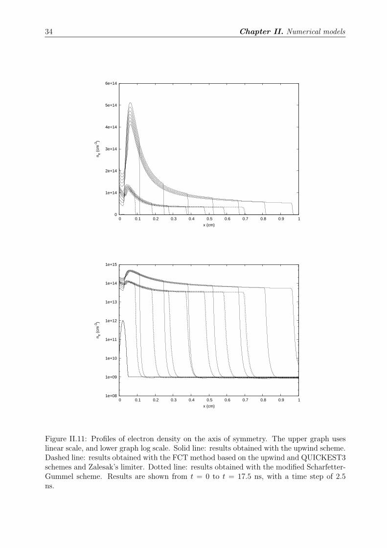
34 Chapter II. Numerical models
0
1e+14
2e+14
3e+14
4e+14
5e+14
6e+14
0 0.1 0.2 0.3 0.4 0.5 0.6 0.7 0.8 0.9 1
n e (
cm-3
)
x (cm)
1e+08
1e+09
1e+10
1e+11
1e+12
1e+13
1e+14
1e+15
0 0.1 0.2 0.3 0.4 0.5 0.6 0.7 0.8 0.9 1
n e (
cm-3
)
x (cm)
Figure II.11: Profiles of electron density on the axis of symmetry. The upper graph useslinear scale, and lower graph log scale. Solid line: results obtained with the upwind scheme.Dashed line: results obtained with the FCT method based on the upwind and QUICKEST3schemes and Zalesak’s limiter. Dotted line: results obtained with the modified Scharfetter-Gummel scheme. Results are shown from t = 0 to t = 17.5 ns, with a time step of 2.5ns.
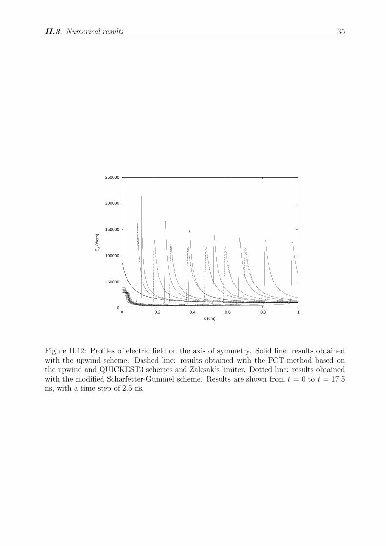
II.3. Numerical results 35
0
50000
100000
150000
200000
250000
0 0.2 0.4 0.6 0.8 1
Ex
(V/c
m)
x (cm)
Figure II.12: Profiles of electric field on the axis of symmetry. Solid line: results obtainedwith the upwind scheme. Dashed line: results obtained with the FCT method based onthe upwind and QUICKEST3 schemes and Zalesak’s limiter. Dotted line: results obtainedwith the modified Scharfetter-Gummel scheme. Results are shown from t = 0 to t = 17.5ns, with a time step of 2.5 ns.
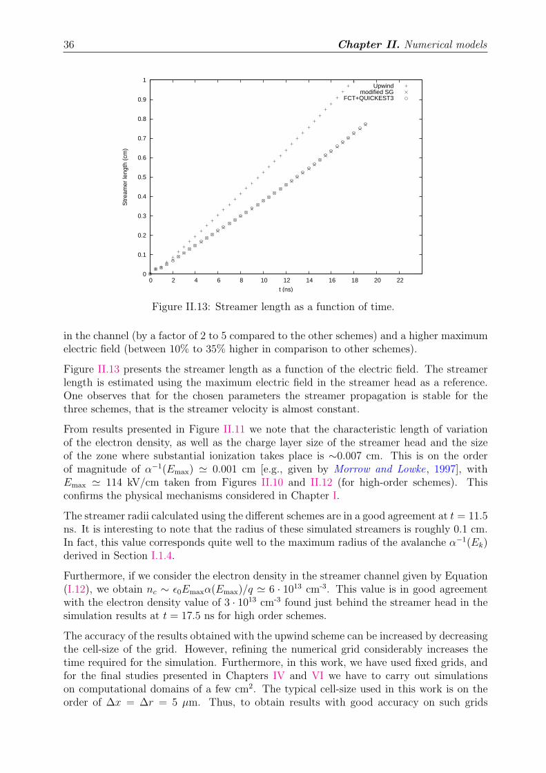
36 Chapter II. Numerical models
0
0.1
0.2
0.3
0.4
0.5
0.6
0.7
0.8
0.9
1
0 2 4 6 8 10 12 14 16 18 20 22
Str
eam
er le
ngth
(cm
)
t (ns)
Upwindmodified SG
FCT+QUICKEST3
Figure II.13: Streamer length as a function of time.
in the channel (by a factor of 2 to 5 compared to the other schemes) and a higher maximumelectric field (between 10% to 35% higher in comparison to other schemes).
Figure II.13 presents the streamer length as a function of the electric field. The streamerlength is estimated using the maximum electric field in the streamer head as a reference.One observes that for the chosen parameters the streamer propagation is stable for thethree schemes, that is the streamer velocity is almost constant.
From results presented in Figure II.11 we note that the characteristic length of variationof the electron density, as well as the charge layer size of the streamer head and the sizeof the zone where substantial ionization takes place is ∼0.007 cm. This is on the orderof magnitude of α−1(Emax) ≃ 0.001 cm [e.g., given by Morrow and Lowke, 1997], withEmax ≃ 114 kV/cm taken from Figures II.10 and II.12 (for high-order schemes). Thisconfirms the physical mechanisms considered in Chapter I.
The streamer radii calculated using the different schemes are in a good agreement at t = 11.5ns. It is interesting to note that the radius of these simulated streamers is roughly 0.1 cm.In fact, this value corresponds quite well to the maximum radius of the avalanche α−1(Ek)derived in Section I.1.4.
Furthermore, if we consider the electron density in the streamer channel given by Equation(I.12), we obtain nc ∼ ǫ0Emaxα(Emax)/q ≃ 6 · 1013 cm-3. This value is in good agreementwith the electron density value of 3 · 1013 cm-3 found just behind the streamer head in thesimulation results at t = 17.5 ns for high order schemes.
The accuracy of the results obtained with the upwind scheme can be increased by decreasingthe cell-size of the grid. However, refining the numerical grid considerably increases thetime required for the simulation. Furthermore, in this work, we have used fixed grids, andfor the final studies presented in Chapters IV and VI we have to carry out simulationson computational domains of a few cm2. The typical cell-size used in this work is on theorder of ∆x = ∆r = 5 µm. Thus, to obtain results with good accuracy on such grids
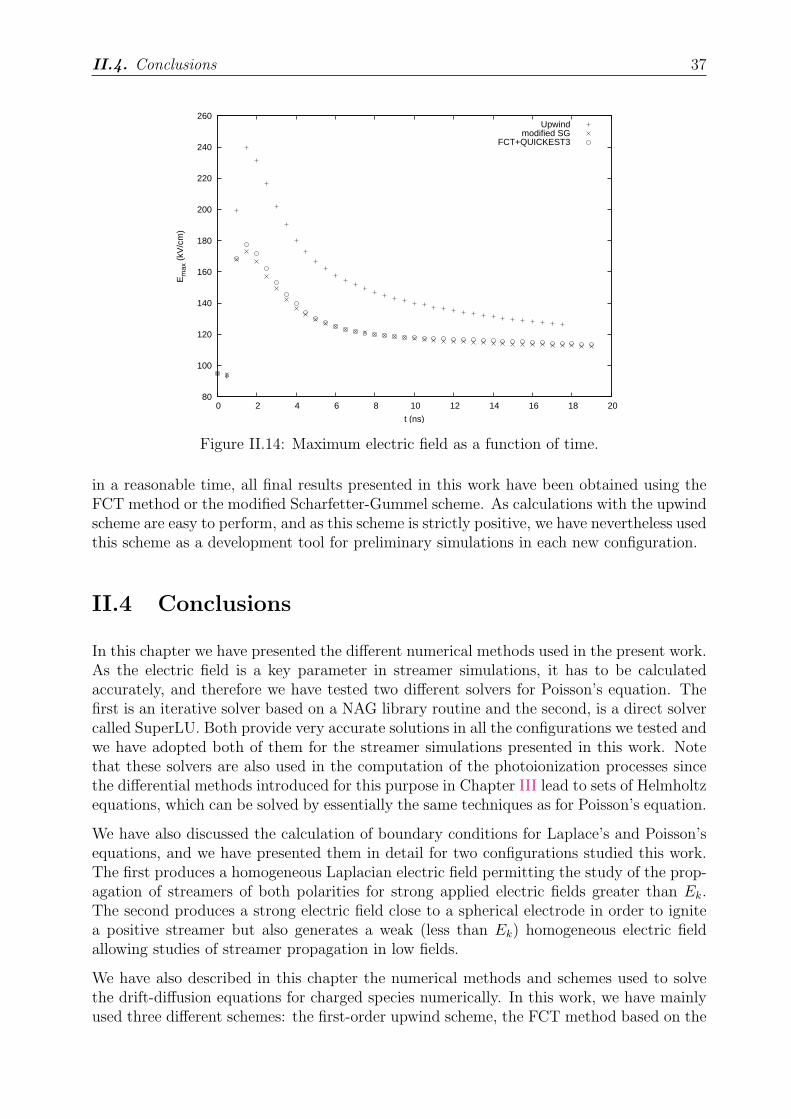
II.4. Conclusions 37
80
100
120
140
160
180
200
220
240
260
0 2 4 6 8 10 12 14 16 18 20
Em
ax (
kV/c
m)
t (ns)
Upwindmodified SG
FCT+QUICKEST3
Figure II.14: Maximum electric field as a function of time.
in a reasonable time, all final results presented in this work have been obtained using theFCT method or the modified Scharfetter-Gummel scheme. As calculations with the upwindscheme are easy to perform, and as this scheme is strictly positive, we have nevertheless usedthis scheme as a development tool for preliminary simulations in each new configuration.
II.4 Conclusions
In this chapter we have presented the different numerical methods used in the present work.As the electric field is a key parameter in streamer simulations, it has to be calculatedaccurately, and therefore we have tested two different solvers for Poisson’s equation. Thefirst is an iterative solver based on a NAG library routine and the second, is a direct solvercalled SuperLU. Both provide very accurate solutions in all the configurations we tested andwe have adopted both of them for the streamer simulations presented in this work. Notethat these solvers are also used in the computation of the photoionization processes sincethe differential methods introduced for this purpose in Chapter III lead to sets of Helmholtzequations, which can be solved by essentially the same techniques as for Poisson’s equation.
We have also discussed the calculation of boundary conditions for Laplace’s and Poisson’sequations, and we have presented them in detail for two configurations studied this work.The first produces a homogeneous Laplacian electric field permitting the study of the prop-agation of streamers of both polarities for strong applied electric fields greater than Ek.The second produces a strong electric field close to a spherical electrode in order to ignitea positive streamer but also generates a weak (less than Ek) homogeneous electric fieldallowing studies of streamer propagation in low fields.
We have also described in this chapter the numerical methods and schemes used to solvethe drift-diffusion equations for charged species numerically. In this work, we have mainlyused three different schemes: the first-order upwind scheme, the FCT method based on the

38 Chapter II. Numerical models
the upwind and QUICKEST3 schemes and Zalesak’s limiter, and the modified Scharfetter-Gummel scheme. In the last section, we have compared the results obtained for a represen-tative model case of propagation of a positive streamer with these three schemes, and wehave demonstrated that the upwind scheme could significantly overestimate the streamervelocity, the electron density and the maximum electric field on grids with typical cellsizes on the order of 5 µm. We demonstrated that to calculate streamer propagation onsuch grids accurately, higher order schemes such as the FCT method and the modifiedScharfetter-Gummel scheme are required. In this section we also demonstrated that someproperties of the simulated positive streamer are in good agreement with simple physicalmodels presented in Chapter I.

Chapter III
Photoionization model
Table of ContentsIII.1 Introduction . . . . . . . . . . . . . . . . . . . . . . . . . . . . . . 40
III.2 Classical integral model for photoionization in air . . . . . . . . 42
III.3 Two and three-exponential Helmholtz models for photoion-ization in air . . . . . . . . . . . . . . . . . . . . . . . . . . . . . . 44
III.4 Three-group Eddington and SP3 approximations for photoion-ization in air . . . . . . . . . . . . . . . . . . . . . . . . . . . . . . 47
III.4.1 Three-group approach . . . . . . . . . . . . . . . . . . . . . . . . 47
III.4.2 Eddington and SP3 models . . . . . . . . . . . . . . . . . . . . . 49
III.4.3 Determination of parameters of the three-group models . . . . . 51
III.5 Boundary conditions . . . . . . . . . . . . . . . . . . . . . . . . . 52
III.5.1 Two and three-exponential Helmholtz models . . . . . . . . . . . 52
III.5.2 Three-group Eddington and SP3 models . . . . . . . . . . . . . . 52
Boundary conditions using the integral Zheleznyak model . . . . 52
Marshak’s boundary conditions for the Eddington model . . . . . 53
Larsen’s boundary conditions for the SP3 model . . . . . . . . . 53
III.6 Results and Discussion . . . . . . . . . . . . . . . . . . . . . . . . 54
III.6.1 Gaussian photoionization source . . . . . . . . . . . . . . . . . . 54
III.6.2 Streamer simulations . . . . . . . . . . . . . . . . . . . . . . . . . 61
Double-headed streamers in air . . . . . . . . . . . . . . . . . . . 63
Propagation of streamer in a weak external field . . . . . . . . . 69
III.7 Conclusions . . . . . . . . . . . . . . . . . . . . . . . . . . . . . . . 73
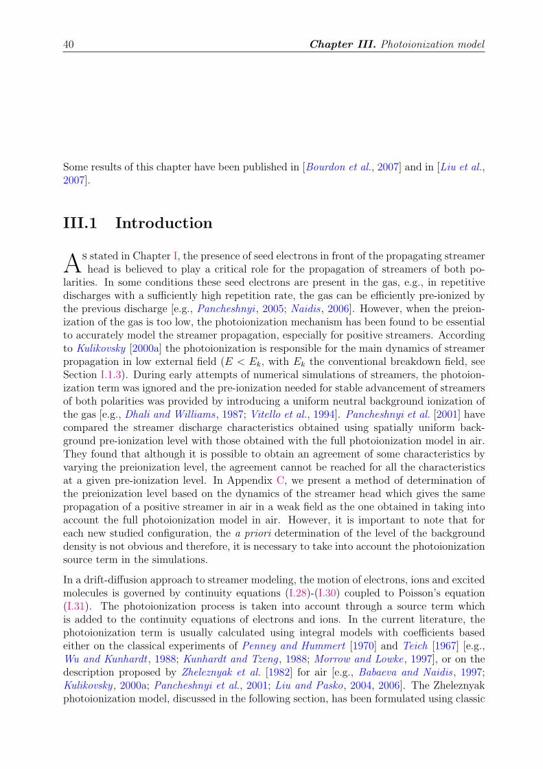
40 Chapter III. Photoionization model
Some results of this chapter have been published in [Bourdon et al., 2007] and in [Liu et al.,2007].
III.1 Introduction
As stated in Chapter I, the presence of seed electrons in front of the propagating streamerhead is believed to play a critical role for the propagation of streamers of both po-
larities. In some conditions these seed electrons are present in the gas, e.g., in repetitivedischarges with a sufficiently high repetition rate, the gas can be efficiently pre-ionized bythe previous discharge [e.g., Pancheshnyi , 2005; Naidis , 2006]. However, when the preion-ization of the gas is too low, the photoionization mechanism has been found to be essentialto accurately model the streamer propagation, especially for positive streamers. Accordingto Kulikovsky [2000a] the photoionization is responsible for the main dynamics of streamerpropagation in low external field (E < Ek, with Ek the conventional breakdown field, seeSection I.1.3). During early attempts of numerical simulations of streamers, the photoion-ization term was ignored and the pre-ionization needed for stable advancement of streamersof both polarities was provided by introducing a uniform neutral background ionization ofthe gas [e.g., Dhali and Williams , 1987; Vitello et al., 1994]. Pancheshnyi et al. [2001] havecompared the streamer discharge characteristics obtained using spatially uniform back-ground pre-ionization level with those obtained with the full photoionization model in air.They found that although it is possible to obtain an agreement of some characteristics byvarying the preionization level, the agreement cannot be reached for all the characteristicsat a given pre-ionization level. In Appendix C, we present a method of determination ofthe preionization level based on the dynamics of the streamer head which gives the samepropagation of a positive streamer in air in a weak field as the one obtained in taking intoaccount the full photoionization model in air. However, it is important to note that foreach new studied configuration, the a priori determination of the level of the backgrounddensity is not obvious and therefore, it is necessary to take into account the photoionizationsource term in the simulations.
In a drift-diffusion approach to streamer modeling, the motion of electrons, ions and excitedmolecules is governed by continuity equations (I.28)-(I.30) coupled to Poisson’s equation(I.31). The photoionization process is taken into account through a source term whichis added to the continuity equations of electrons and ions. In the current literature, thephotoionization term is usually calculated using integral models with coefficients basedeither on the classical experiments of Penney and Hummert [1970] and Teich [1967] [e.g.,Wu and Kunhardt , 1988; Kunhardt and Tzeng , 1988; Morrow and Lowke, 1997], or on thedescription proposed by Zheleznyak et al. [1982] for air [e.g., Babaeva and Naidis , 1997;Kulikovsky , 2000a; Pancheshnyi et al., 2001; Liu and Pasko, 2004, 2006]. The Zheleznyakphotoionization model, discussed in the following section, has been formulated using classic
III.1. Introduction 41
experimental data obtained at low pressure [Penney and Hummert , 1970; Teich, 1967].However, this model agrees well with results of more recent experiments at atmosphericpressure [Aints et al., 2008; Naidis , 2006, and references cited therein].
For the integral approach mentioned above, the calculation of the photoionization sourceterm at a given point of the volume studied requires a quadrature over the complete volumeof the discharge. Therefore, the calculation of the photoionization source term in streamerdischarges is computationally expensive. To accelerate the simulation of streamers, differentapproximations have been proposed in the literature to reduce the computation time spenton calculation of the photoionization source term [Kulikovsky , 2000a; Hallac et al., 2003;Pancheshnyi et al., 2001]. Kulikovsky [2000a] proposed to confine the emitting volumeof the photoionizing radiation to a small cylinder around the main axis of the dischargeand to divide it into small rings. For a two-dimensional modeling of streamers assumingcylindrical symmetry, the effects of an emitting ring at a point of interest can be effectivelycharacterized by their relative locations (described by a geometric factor in [Kulikovsky ,2000a]). This geometric factor only needs to be calculated once before the simulation fora specific computational geometry and can be repeatedly reused in the simulations. In[Kulikovsky , 2000a] and [Hallac et al., 2003] photoionization is calculated on a coarse gridand interpolation is used to obtain needed values on the main grid. Finally, in [Pancheshnyiet al., 2001] calculations are carried out in a small area around the streamer head. Wenote that all the approximate models reviewed above reduce the computation time to acertain degree but the accuracy of these models has not yet been rigorously evaluated anddemonstrated in the existing literature.
Recently, two different approaches to calculate the photoionization term have been proposedto avoid the calculation of the global quadrature over the simulation domain. The firstapproach was tested a few years ago [Djermoune et al., 1995a, b] and improved recently[Ségur et al., 2006]. This method is based on the direct numerical solution of an improvedEddington approximation of the radiative transfer equation. The second approach hasbeen proposed recently by Luque et al. [2007]. These authors proposed to approximatethe absorption function of the gas in order to transform the integral expression of thephotoionization term into a set of Helmholtz differential equations. In this chapter, wepresent and discuss these two approaches for the calculation of the photoionization term,and develop improved models based on the same principles by more accurately accountingfor the spectral dependence of the photoionization. We also discuss the importance ofaccurate calculation of boundary conditions for the photoionization term and we introduceboundary conditions based on the integral Zheleznyak model and boundary conditionsbased on radiative transfer theory. The validity and range of applicability of the developedmodels for the photoionization term is demonstrated by performing direct comparisonsof the results from these models and results obtained from the classic integral model ofZheleznyak et al. [1982]. First, specific validation comparisons are presented for a set ofartificial sources of photoionizing radiation with different Gaussian dimensions. Then, wepresent validation comparisons for the development of a double-headed streamer in a highelectric field (>Ek) at ground pressure and for the positive streamer propagation in weakexternal electric fields (<Ek) at ground pressure, i.e., conditions which are of great interestfor practical applications.
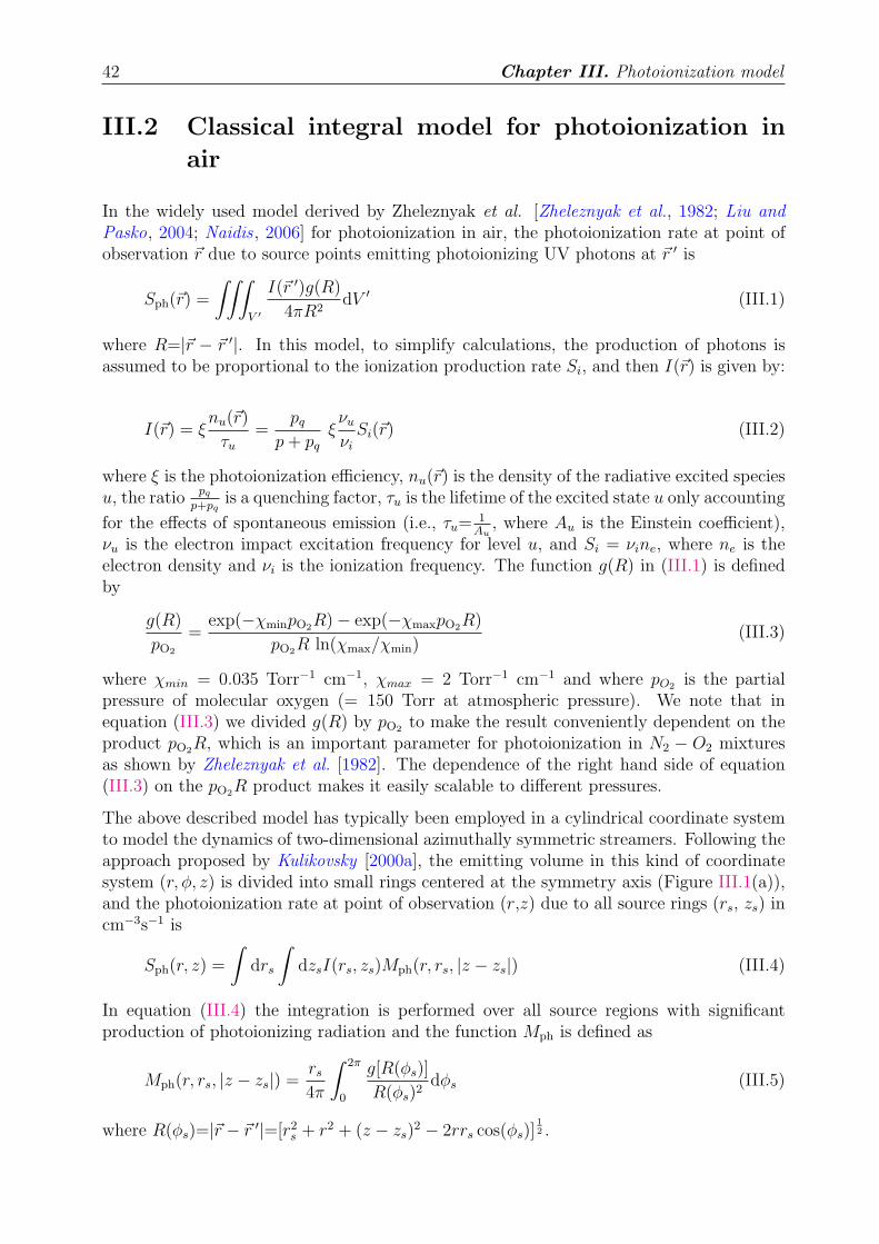
42 Chapter III. Photoionization model
III.2 Classical integral model for photoionization inair
In the widely used model derived by Zheleznyak et al. [Zheleznyak et al., 1982; Liu andPasko, 2004; Naidis , 2006] for photoionization in air, the photoionization rate at point ofobservation ~r due to source points emitting photoionizing UV photons at ~r ′ is
Sph(~r) =
∫∫∫
V ′
I(~r ′)g(R)
4πR2dV ′ (III.1)
where R=|~r − ~r ′|. In this model, to simplify calculations, the production of photons isassumed to be proportional to the ionization production rate Si, and then I(~r) is given by:
I(~r) = ξnu(~r)
τu
=pq
p + pq
ξνu
νi
Si(~r) (III.2)
where ξ is the photoionization efficiency, nu(~r) is the density of the radiative excited speciesu, the ratio pq
p+pqis a quenching factor, τu is the lifetime of the excited state u only accounting
for the effects of spontaneous emission (i.e., τu= 1Au
, where Au is the Einstein coefficient),νu is the electron impact excitation frequency for level u, and Si = νine, where ne is theelectron density and νi is the ionization frequency. The function g(R) in (III.1) is definedby
g(R)
pO2
=exp(−χminpO2
R) − exp(−χmaxpO2R)
pO2R ln(χmax/χmin)
(III.3)
where χmin = 0.035 Torr−1 cm−1, χmax = 2 Torr−1 cm−1 and where pO2is the partial
pressure of molecular oxygen (= 150 Torr at atmospheric pressure). We note that inequation (III.3) we divided g(R) by pO2
to make the result conveniently dependent on theproduct pO2
R, which is an important parameter for photoionization in N2 − O2 mixturesas shown by Zheleznyak et al. [1982]. The dependence of the right hand side of equation(III.3) on the pO2
R product makes it easily scalable to different pressures.
The above described model has typically been employed in a cylindrical coordinate systemto model the dynamics of two-dimensional azimuthally symmetric streamers. Following theapproach proposed by Kulikovsky [2000a], the emitting volume in this kind of coordinatesystem (r, φ, z) is divided into small rings centered at the symmetry axis (Figure III.1(a)),and the photoionization rate at point of observation (r,z) due to all source rings (rs, zs) incm−3s−1 is
Sph(r, z) =
∫
drs
∫
dzsI(rs, zs)Mph(r, rs, |z − zs|) (III.4)
In equation (III.4) the integration is performed over all source regions with significantproduction of photoionizing radiation and the function Mph is defined as
Mph(r, rs, |z − zs|) =rs
4π
∫ 2π
0
g[R(φs)]
R(φs)2dφs (III.5)
where R(φs)=|~r − ~r ′|=[r2s + r2 + (z − zs)
2 − 2rrs cos(φs)]1
2 .
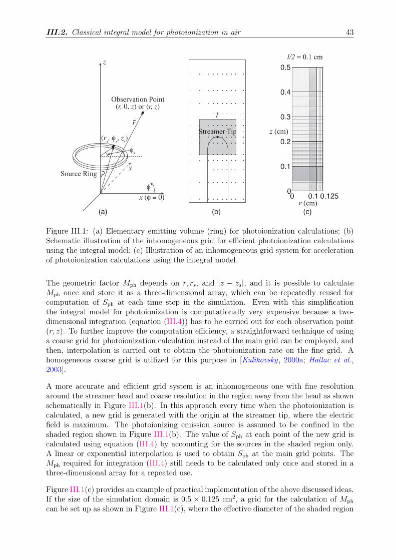
III.2. Classical integral model for photoionization in air 43
(a) (b)
y
z
x (φ = 0)
φ
φs
(r, 0, z) or (r, z)
(rs, φ
s, z
s)
Observation Point
Source Ring
0 0.1 0.1250
0.1
0.2
0.3
z (cm)
r (cm)
0.4
0.5
(c)
l/2 = 0.1 cm
Streamer Tip
l
r
r’
Figure III.1: (a) Elementary emitting volume (ring) for photoionization calculations; (b)Schematic illustration of the inhomogeneous grid for efficient photoionization calculationsusing the integral model; (c) Illustration of an inhomogeneous grid system for accelerationof photoionization calculations using the integral model.
The geometric factor Mph depends on r, rs, and |z − zs|, and it is possible to calculateMph once and store it as a three-dimensional array, which can be repeatedly reused forcomputation of Sph at each time step in the simulation. Even with this simplificationthe integral model for photoionization is computationally very expensive because a two-dimensional integration (equation (III.4)) has to be carried out for each observation point(r, z). To further improve the computation efficiency, a straightforward technique of usinga coarse grid for photoionization calculation instead of the main grid can be employed, andthen, interpolation is carried out to obtain the photoionization rate on the fine grid. Ahomogeneous coarse grid is utilized for this purpose in [Kulikovsky , 2000a; Hallac et al.,2003].
A more accurate and efficient grid system is an inhomogeneous one with fine resolutionaround the streamer head and coarse resolution in the region away from the head as shownschematically in Figure III.1(b). In this approach every time when the photoionization iscalculated, a new grid is generated with the origin at the streamer tip, where the electricfield is maximum. The photoionizing emission source is assumed to be confined in theshaded region shown in Figure III.1(b). The value of Sph at each point of the new grid iscalculated using equation (III.4) by accounting for the sources in the shaded region only.A linear or exponential interpolation is used to obtain Sph at the main grid points. TheMph required for integration (III.4) still needs to be calculated only once and stored in athree-dimensional array for a repeated use.
Figure III.1(c) provides an example of practical implementation of the above discussed ideas.If the size of the simulation domain is 0.5 × 0.125 cm2, a grid for the calculation of Mph
can be set up as shown in Figure III.1(c), where the effective diameter of the shaded region
44 Chapter III. Photoionization model
shown in Figure III.1(b) is assumed to be l = 0.2 cm. In the z direction the simulationdomain is divided in equal intervals with length l/2=0.1 cm. The grid size in each of theseintervals is constant, and increases exponentially with the distance from the origin fromone interval to the next. If the grid size in a particular interval becomes greater than theinterval itself (l/2), then l/2 is used as the grid size instead, as shown, for example forthe interval from z=0.4 to 0.5 cm in Figure III.1(c). The grid in r direction is generatedfollowing the same procedure. Mph can then be calculated on this grid using equation(III.5). The grid for the problem geometry shown in Figure III.1(b) can be generated byfollowing the same ideas with the origin placed at the streamer tip and with the l/2 intervalswith reduced grid resolution extending in both positive and negative z directions from theshaded region. The calculation of the contribution to Sph(r, z) due to a source ring at (rs, zs)is significantly accelerated by a simple call of the corresponding pre-calculated element ofthe three-dimensional matrix Mph(r, rs, |z − zs|). Finally, the contributions from all therings constituting the shaded source shown in Figure III.1(b) are summed up to obtain thetotal Sph(r, z).
The integral approach with variable size grids based on Zheleznyak et al. [1982] modeloutlined above is used for streamer calculations reported in Section III.6.2 of the presentchapter. It should be noted that for the double-headed streamer presented in Section III.6.2,there are two grid systems generated with the origin of each grid system positioned at thetip of the corresponding streamer head. However, the same precalculated Mph matrix isused for both heads.
III.3 Two and three-exponential Helmholtz models forphotoionization in air
Luque et al. [2007] have recently proposed a novel approach allowing to effectively replacethe calculation of integral (III.1) of the classic photoionization model with a solution ofa set of Helmholtz differential equations, which can be very efficiently solved using welldeveloped techniques available for solution of the elliptic partial differential equations. Interms of notations adopted in the present chapter the approach proposed by Luque et al.[2007] involves fitting of the g(R)/R ratio in (III.1) with a sum of exponential functionsleading to a set of integrals, each of which can effectively be interpreted as an integralsolution of a separate Helmholtz differential equation. After this equivalent representation isestablished the problem can be solved by solving the set of Helmholtz differential equations,instead of direct evaluation of integrals. However, the two-exponential fit provided in [Luqueet al., 2007] has been applied to low pressure experimental data of Penney and Hummert[1970] effectively corresponding to the function g(R), rather than to g(R)/R required forthe correct solution of the problem. In this section we present correct solution of thisproblem using two and three-exponential fits. In Section III.6.1 we demonstrate that thetwo-exponential fit is generally not sufficient and the three-exponential fit is needed forobtaining the accurate solution of the problem for a full range of pO2
R values in which theZheleznyak et al. [1982] photoionization model remains valid.
We note that the Zheleznyak et al. [1982] photoionization model, discussed in the previoussection, has been formulated using experimental data obtained at low pressure [Penneyand Hummert , 1970; Teich, 1967] and agrees well with results of more recent experiments
III.3. Two and three-exponential Helmholtz models for photoionization in air 45
Table III.1: Parameters of the two-exponential fit of g(R)/pO2/(pO2
R) as a function ofpO2
R.
j Aj [cm−2 Torr−2] λj [cm−1 Torr−1]1 0.0021 0.09742 0.1775 0.5877
Table III.2: Parameters of the three-exponential fit of g(R)/pO2/(pO2
R) as a function pO2R.
j Aj [cm−2 Torr−2] λj [cm−1 Torr−1]1 1.986×10⁻⁴ 0.05532 0.0051 0.14603 0.4886 0.89
at atmospheric pressure [Aints et al., 2008; Naidis , 2006, and references cited therein].Therefore, in contrast to [Luque et al., 2007] in our derivation below we do not employthe low pressure data of Penney and Hummert [1970], but rather formulate the two andthree-exponential Helmholtz models using the g(R) function (III.3) appearing in the classicintegral model for photoionization in air [Zheleznyak et al., 1982].
The function Sph(~r) given by (III.1) can be represented in the form
Sph(~r) =∑
j
Sjph(~r) (III.6)
with terms
Sjph(~r) =
∫∫∫
V ′
I(~r ′)Ajp2O2
e−λjpO2R
4πRdV ′ (III.7)
satisfying Helmholtz differential equations
∇2Sjph(~r) − (λjpO2
)2Sjph(~r) = −Ajp
2O2
I(~r) (III.8)
Having compared equations (III.1) and (III.7) it can be easily verified that
g(R)
pO2
= (pO2R)∑
j
Aje−λjpO2
R (III.9)
The solution of the problem requires fitting of the function g(R)/pO2by series of exponents
multiplied by (pO2R). After the fitting, the photoionization problem can be solved by solving
differential equations (III.8) and performing summation (III.6). In practice, it appears tobe easier to fit function g(R)/pO2
/(pO2R) with a sum of exponents
∑
j Aje−λjpO2
R and thenmultiply the result by (pO2
R) to obtain the desired representation of g(R)/pO2given by
(III.9).
The function g(R)/pO2is shown in Figure III.2 by solid line and a two-exponential fit
performed by MATLAB function fminsearch (based on Nelder-Mead simplex direct searchmethod) is shown by the dashed line. The two-exponential fit was performed for the range
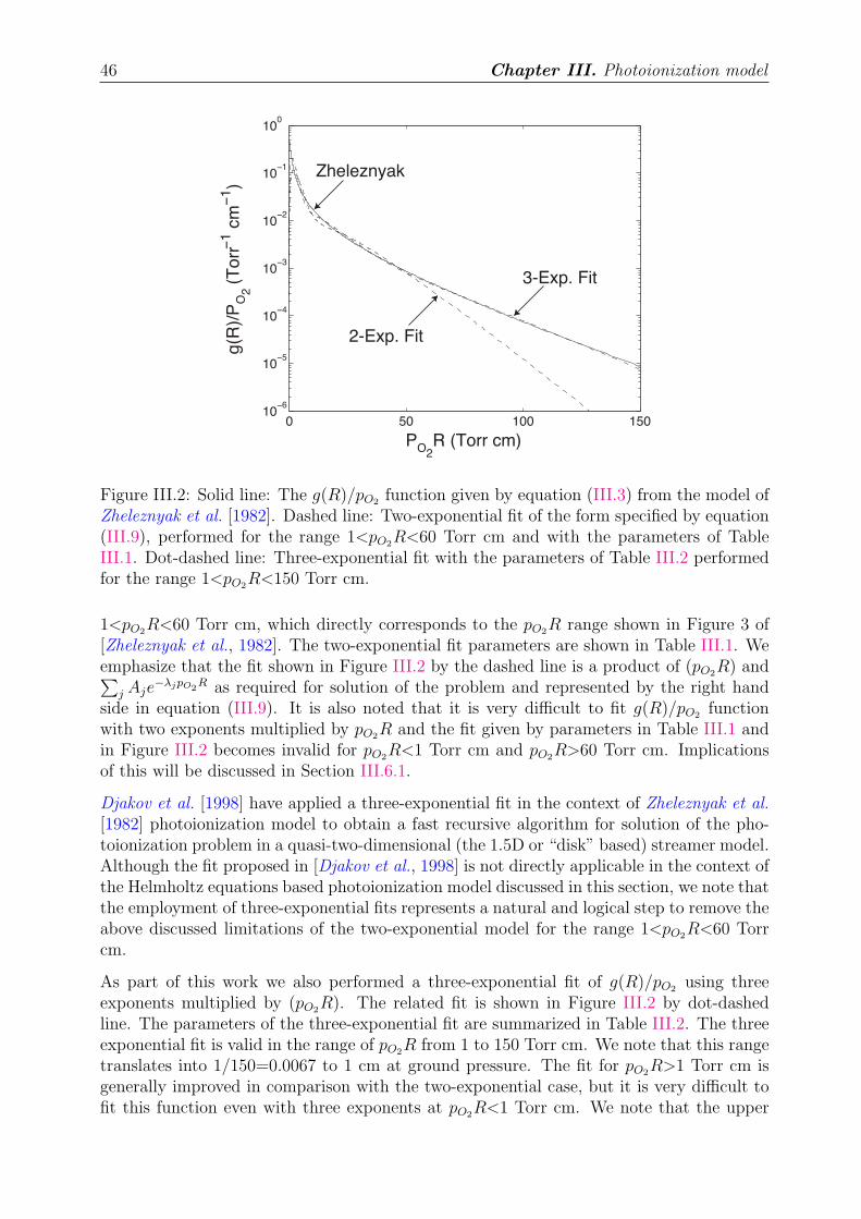
46 Chapter III. Photoionization model
0 50 100 15010
−6
10−5
10−4
10−3
10−2
10−1
100
g(R)/PO2 (Torr−1 cm−1)
PO2R (Torr cm)
Zheleznyak
2-Exp. Fit
3-Exp. Fit
Figure III.2: Solid line: The g(R)/pO2function given by equation (III.3) from the model of
Zheleznyak et al. [1982]. Dashed line: Two-exponential fit of the form specified by equation(III.9), performed for the range 1<pO2
R<60 Torr cm and with the parameters of TableIII.1. Dot-dashed line: Three-exponential fit with the parameters of Table III.2 performedfor the range 1<pO2
R<150 Torr cm.
1<pO2R<60 Torr cm, which directly corresponds to the pO2
R range shown in Figure 3 of[Zheleznyak et al., 1982]. The two-exponential fit parameters are shown in Table III.1. Weemphasize that the fit shown in Figure III.2 by the dashed line is a product of (pO2
R) and∑
j Aje−λjpO2
R as required for solution of the problem and represented by the right handside in equation (III.9). It is also noted that it is very difficult to fit g(R)/pO2
functionwith two exponents multiplied by pO2
R and the fit given by parameters in Table III.1 andin Figure III.2 becomes invalid for pO2
R<1 Torr cm and pO2R>60 Torr cm. Implications
of this will be discussed in Section III.6.1.
Djakov et al. [1998] have applied a three-exponential fit in the context of Zheleznyak et al.[1982] photoionization model to obtain a fast recursive algorithm for solution of the pho-toionization problem in a quasi-two-dimensional (the 1.5D or “disk” based) streamer model.Although the fit proposed in [Djakov et al., 1998] is not directly applicable in the context ofthe Helmholtz equations based photoionization model discussed in this section, we note thatthe employment of three-exponential fits represents a natural and logical step to remove theabove discussed limitations of the two-exponential model for the range 1<pO2
R<60 Torrcm.
As part of this work we also performed a three-exponential fit of g(R)/pO2using three
exponents multiplied by (pO2R). The related fit is shown in Figure III.2 by dot-dashed
line. The parameters of the three-exponential fit are summarized in Table III.2. The threeexponential fit is valid in the range of pO2
R from 1 to 150 Torr cm. We note that this rangetranslates into 1/150=0.0067 to 1 cm at ground pressure. The fit for pO2
R>1 Torr cm isgenerally improved in comparison with the two-exponential case, but it is very difficult tofit this function even with three exponents at pO2
R<1 Torr cm. We note that the upper
III.4. Three-group Eddington and SP3 approximations for photoionization in air 47
limit of validity of the developed three-exponential fit (pO2R=150 Torr cm) exceeds the
pO2R≃100 Torr cm (i.e., pR≃500 Torr cm, where p is air pressure) validity threshold of the
Zheleznyak et al. [1982] model for photoionization in air, as discussed recently in [Naidis ,2006].
The accurate numerical solution of Helmholtz equations (III.8) requires knowledge aboutvalues of Sj
ph(~r) functions at the boundaries of the simulation domain. The determinationof boundary conditions will be presented and discussed in Section III.5.
III.4 Three-group Eddington and SP3 approximationsfor photoionization in air
III.4.1 Three-group approach
In [Ségur et al., 2006], the photoionization source term Sph(~r) is calculated using directnumerical solutions of the first (also called Eddington approximation) and the third order(also called SP3) approximations of the radiative transfer equation. Ségur et al. [2006]introduce a simple monochromatic approach (also called one-group method) and derive thephysical parameters required for applying this method to calculate Sph(~r) for non-thermalgas discharges in air at atmospheric pressure by making the model results as consistent aspossible with the classical Zheleznyak model.
In order to achieve a better agreement with the Zheleznyak model for the Eddington andSP3 approximations, we propose to consider j = 1, Ng effective monochromatic radiativetransfer equations. We consider that there is no photon scattering and as the timescale ofphoton propagation is much less than the timescale of streamer propagation, we neglectthe transient term of the radiative transfer equation. For each frequency, the effectivemonochromatic radiative transfer equation can be written as [Ségur et al., 2006]:
~Ω · ~∇Ψj(~r, ~Ω) + λjpO2Ψj(~r, ~Ω) =
nu(~r)
4πcτu
(III.10)
where to simplify the notation, first, the time dependent functions Ψj(~r, ~Ω, t) and nu(~r, t)
are noted as Ψj(~r, ~Ω) and nu(~r) and second, only one radiative excited state u is consid-ered. The quantity λjpO2
is the absorption coefficient. It is important to mention that allmonochromatic equations for j = 1, Ng have the same source term but different absorptioncoefficients. The equation (III.10) can be simply integrated to derive Ψ0,j(~r), the isotropicpart of the photon distribution function Ψj(~r, ~Ω) as:
Ψ0,j(~r) =
∫∫∫
V ′
nu(~r′)
cτu
exp(−λjpO2R)
4πR2dV ′ (III.11)
Then we assume that the isotropic part of the total distribution function Ψ0(~r) can bewritten as:
Ψ0(~r) =∑
j
αjΨ0,j(~r) (III.12)
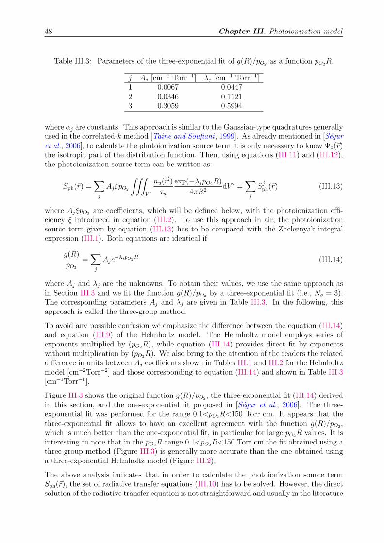
48 Chapter III. Photoionization model
Table III.3: Parameters of the three-exponential fit of g(R)/pO2as a function pO2
R.
j Aj [cm−1 Torr−1] λj [cm−1 Torr−1]1 0.0067 0.04472 0.0346 0.11213 0.3059 0.5994
where αj are constants. This approach is similar to the Gaussian-type quadratures generallyused in the correlated-k method [Taine and Soufiani , 1999]. As already mentioned in [Séguret al., 2006], to calculate the photoionization source term it is only necessary to know Ψ0(~r)the isotropic part of the distribution function. Then, using equations (III.11) and (III.12),the photoionization source term can be written as:
Sph(~r) =∑
j
AjξpO2
∫∫∫
V ′
nu(~r′)
τu
exp(−λjpO2R)
4πR2dV ′ =
∑
j
Sjph(~r) (III.13)
where AjξpO2are coefficients, which will be defined below, with the photoionization effi-
ciency ξ introduced in equation (III.2). To use this approach in air, the photoionizationsource term given by equation (III.13) has to be compared with the Zheleznyak integralexpression (III.1). Both equations are identical if
g(R)
pO2
=∑
j
Aje−λjpO2
R (III.14)
where Aj and λj are the unknowns. To obtain their values, we use the same approach asin Section III.3 and we fit the function g(R)/pO2
by a three-exponential fit (i.e., Ng = 3).The corresponding parameters Aj and λj are given in Table III.3. In the following, thisapproach is called the three-group method.
To avoid any possible confusion we emphasize the difference between the equation (III.14)and equation (III.9) of the Helmholtz model. The Helmholtz model employs series ofexponents multiplied by (pO2
R), while equation (III.14) provides direct fit by exponentswithout multiplication by (pO2
R). We also bring to the attention of the readers the relateddifference in units between Aj coefficients shown in Tables III.1 and III.2 for the Helmholtzmodel [cm−2Torr−2] and those corresponding to equation (III.14) and shown in Table III.3[cm−1Torr−1].
Figure III.3 shows the original function g(R)/pO2, the three-exponential fit (III.14) derived
in this section, and the one-exponential fit proposed in [Ségur et al., 2006]. The three-exponential fit was performed for the range 0.1<pO2
R<150 Torr cm. It appears that thethree-exponential fit allows to have an excellent agreement with the function g(R)/pO2
,which is much better than the one-exponential fit, in particular for large pO2
R values. It isinteresting to note that in the pO2
R range 0.1<pO2R<150 Torr cm the fit obtained using a
three-group method (Figure III.3) is generally more accurate than the one obtained usinga three-exponential Helmholtz model (Figure III.2).
The above analysis indicates that in order to calculate the photoionization source termSph(~r), the set of radiative transfer equations (III.10) has to be solved. However, the directsolution of the radiative transfer equation is not straightforward and usually in the literature
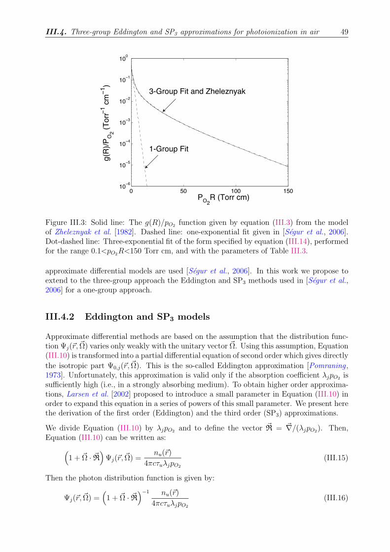
III.4. Three-group Eddington and SP3 approximations for photoionization in air 49
0 50 100 15010
−6
10−5
10−4
10−3
10−2
10−1
100
PO2
R (Torr cm)
g(R
)/P
O2 (
Torr
−1 c
m−1
)
3-Group Fit and Zheleznyak
1-Group Fit
Figure III.3: Solid line: The g(R)/pO2function given by equation (III.3) from the model
of Zheleznyak et al. [1982]. Dashed line: one-exponential fit given in [Ségur et al., 2006].Dot-dashed line: Three-exponential fit of the form specified by equation (III.14), performedfor the range 0.1<pO2
R<150 Torr cm, and with the parameters of Table III.3.
approximate differential models are used [Ségur et al., 2006]. In this work we propose toextend to the three-group approach the Eddington and SP3 methods used in [Ségur et al.,2006] for a one-group approach.
III.4.2 Eddington and SP3 models
Approximate differential methods are based on the assumption that the distribution func-tion Ψj(~r, ~Ω) varies only weakly with the unitary vector ~Ω. Using this assumption, Equation(III.10) is transformed into a partial differential equation of second order which gives directlythe isotropic part Ψ0,j(~r, ~Ω). This is the so-called Eddington approximation [Pomraning ,1973]. Unfortunately, this approximation is valid only if the absorption coefficient λjpO2
issufficiently high (i.e., in a strongly absorbing medium). To obtain higher order approxima-tions, Larsen et al. [2002] proposed to introduce a small parameter in Equation (III.10) inorder to expand this equation in a series of powers of this small parameter. We present herethe derivation of the first order (Eddington) and the third order (SP3) approximations.
We divide Equation (III.10) by λjpO2and to define the vector ~R = ~∇/(λjpO2
). Then,Equation (III.10) can be written as:
(
1 + ~Ω · ~R)
Ψj(~r, ~Ω) =nu(~r)
4πcτuλjpO2
(III.15)
Then the photon distribution function is given by:
Ψj(~r, ~Ω) =(
1 + ~Ω · ~R)−1 nu(~r)
4πcτuλjpO2
(III.16)
50 Chapter III. Photoionization model
and by developping into Neumann series, one obtains:
Ψj(~r, ~Ω) =[
1 − ~Ω · ~R + (~Ω · ~R)2 − (~Ω · ~R)3 + · · ·] nu(~r)
4πcτuλjpO2
(III.17)
Thus, the isotropic part of the photon distribution function is given by:
Ψ0,j(~r) =
∫
Ω
Ψj(~r, ~Ω)dΩ =
(
1 +1
3~R2 +
1
5~R4 + · · ·
)
nu(~r)
cτuλjpO2
(III.18)
and then, finally, Equation (III.10) becomes :(
1 − 1
3~R2 − 4
45~R4 − 44
945~R6 − · · ·
)
Ψ0,j(~r) =nu(~r)
cτuλjpO2
(III.19)
Equation (III.19) shows that when the parameter
|~R2Ψ0,j(~r)|Ψ0,j(~r)
≪ 1,
that is under a weak anisotropy assumption, one can truncate the operator series.
For j = 1, Ng, the Eddington approximation of (III.10) to derive Ψ0,j is given by thetruncation to the second term of operator factors in Equation III.19 [Ségur et al., 2006]:
[∇2 − 3(λjpO2)2]ΨED,0,j(~r) = −3λjpO2
nu(~r)
cτu
(III.20)
where ΨED,0,j(~r) represents the first order Eddington approximation of Ψ0,j(~r). It is in-teresting to note that equation (III.20) is an elliptic equation, which has a structure verysimilar to Poisson’s equation. Therefore, as noted in Section II.4, both Poisson’s equationand the Eddington approximation can be solved with the same numerical routine.
In [Larsen et al., 2002], a significant improvement of the accuracy of the solution wasobtained by keeping the terms in the left hand side of equation (III.19) up to the thirdorder Laplacian. In this case, the equation is a partial differential equation of sixth orderwhich can be written as a set of two equations of second order verified by the functions φ1,j
and φ2,j given by:
∇2φ1,j(~r) −(λjpO2
)2
κ21
φ1,j(~r) = −λjpO2
κ21
nu(~r)
cτu
(III.21)
∇2φ2,j(~r) −(λjpO2
)2
κ22
φ2,j(~r) = −λjpO2
κ22
nu(~r)
cτu
(III.22)
where κ21 = 3
7− 2
7
√
65
and κ22 = 3
7+ 2
7
√
65. Then, for j=1, Ng, the third order SP3 approxi-
mation of Ψ0,j is denoted as ΨSP3,0,j and is given by [Larsen et al., 2002]:
ΨSP3,0,j(~r) =γ2φ1,j − γ1φ2,j
γ2 − γ1
(III.23)
III.4. Three-group Eddington and SP3 approximations for photoionization in air 51
where
γn =5
7
[
1 + (−1)n3
√
6
5
]
(III.24)
Equations (III.21) and (III.22) again have the same structure as Poisson’s equation and canbe solved using the same numerical methods.
After obtaining the solution for ΨED,0,j or ΨSP3,0,j, the photoionization source term can becalculated using
Sph(~r) =∑
j
AjξpO2cΨ0,j(~r) =
∑
j
Sjph(~r) (III.25)
by replacing Ψ0,j with ΨED,0,j or ΨSP3,0,j.
It is important to note that equation (III.20) of the Eddington model, and equations (III.21)and (III.22) of the SP3 model are Helmholtz equations of the same structure as equations(III.8). Then the accurate numerical solution of all these equations requires knowledgeabout values of Sj
ph(~r) functions at the boundaries of the simulation domain. The determi-nation of boundary conditions for the different models will be presented and discussed inSection III.5.
Finally, as equations of the Eddington, SP3 and Helmholtz models have the same structure,in Appendix B we show that all solutions of these models can be written in essentiallysame mathematical form, with differences between these models only arising from differentnumerical values of the model coefficients. Then we demonstrate that the three-exponentialHelmholtz model is more accurate than the three-group Eddington model. In Appendix Bwe also demonstrate that the SP3 model can be effectively represented in a mathematicalform equivalent to six-exponential Helmholtz model. This analysis clearly demonstratesthat the three-group SP3 model is more accurate than the three-group Eddington modeland the three-exponential Helmholtz model.
III.4.3 Determination of parameters of the three-group models
The formulation of the above Eddington and SP3 models require separate evaluations of ξin equation (III.25), and nu(~r)
τuin equation (III.20) for the first order approximation, or in
equations (III.21) and (III.22) for the third one. For Zheleznyak and Helmholtz models,the product ξ nu(~r)
τuis computed using equation (III.2) to give the photoionization radiation
source utilizing the known term ξ νu
νigiven by Zheleznyak et al. [1982]. To effectively use the
same term in the Eddington approximations, we can slightly change the above formulationby multiplying both sides of the equation (III.20) or equations (III.21) and (III.22) by aconstant ξ. For example, the following equation is obtained for the first order Eddingtonapproximation:
[∇2 − 3(λjpO2)2][ξΨED,0,j(~r)] = −3λjpO2
ξnu(~r)
cτu
(III.26)
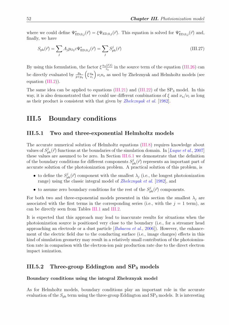
52 Chapter III. Photoionization model
where we could define Ψ∗ED,0,j(~r) = ξΨED,0,j(~r). This equation is solved for Ψ∗
ED,0,j(~r) and,finally, we have
Sph(~r) =∑
j
AjpO2cΨ∗
ED,0,j(~r) =∑
j
Sjph(~r) (III.27)
By using this formulation, the factor ξ nu(~r,t)τu
in the source term of the equation (III.26) can
be directly evaluated by pq
p+pq
(
ξ νu
νi
)
νine as used by Zheleznyak and Helmholtz models (see
equation (III.2)).
The same idea can be applied to equations (III.21) and (III.22) of the SP3 model. In thisway, it is also demonstrated that we could use different combinations of ξ and νu/νi as longas their product is consistent with that given by Zheleznyak et al. [1982].
III.5 Boundary conditions
III.5.1 Two and three-exponential Helmholtz models
The accurate numerical solution of Helmholtz equations (III.8) requires knowledge aboutvalues of Sj
ph(~r) functions at the boundaries of the simulation domain. In [Luque et al., 2007]these values are assumed to be zero. In Section III.6.1 we demonstrate that the definitionof the boundary conditions for different components Sj
ph(~r) represents an important part ofaccurate solution of the photoionization problem. A practical solution of this problem, is
• to define the Sjph(~r) component with the smallest λj (i.e., the longest photoionization
range) using the classic integral model of Zheleznyak et al. [1982], and
• to assume zero boundary conditions for the rest of the Sjph(~r) components.
For both two and three-exponential models presented in this section the smallest λj areassociated with the first terms in the corresponding series (i.e., with the j = 1 term), ascan be directly seen from Tables III.1 and III.2.
It is expected that this approach may lead to inaccurate results for situations when thephotoionization source is positioned very close to the boundary (i.e., for a streamer headapproaching an electrode or a dust particle [Babaeva et al., 2006]). However, the enhance-ment of the electric field due to the conducting surface (i.e., image charges) effects in thiskind of simulation geometry may result in a relatively small contribution of the photoioniza-tion rate in comparison with the electron-ion pair production rate due to the direct electronimpact ionization.
III.5.2 Three-group Eddington and SP3 models
Boundary conditions using the integral Zheleznyak model
As for Helmholtz models, boundary conditions play an important role in the accurateevaluation of the Sph term using the three-group Eddington and SP3 models. It is interesting
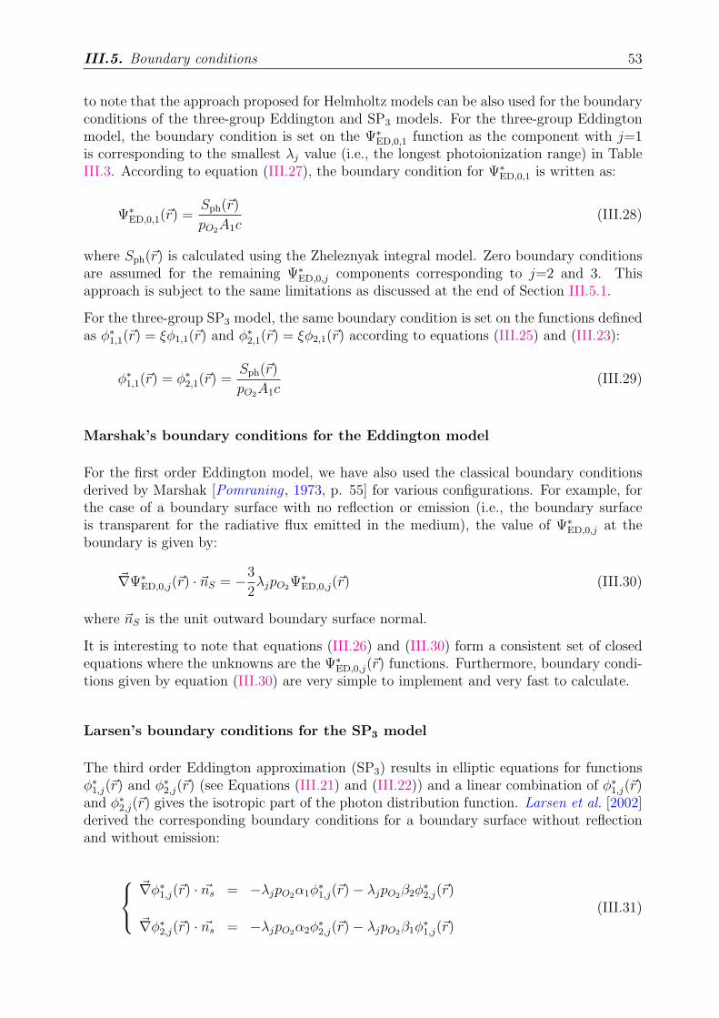
III.5. Boundary conditions 53
to note that the approach proposed for Helmholtz models can be also used for the boundaryconditions of the three-group Eddington and SP3 models. For the three-group Eddingtonmodel, the boundary condition is set on the Ψ∗
ED,0,1 function as the component with j=1is corresponding to the smallest λj value (i.e., the longest photoionization range) in TableIII.3. According to equation (III.27), the boundary condition for Ψ∗
ED,0,1 is written as:
Ψ∗ED,0,1(~r) =
Sph(~r)
pO2A1c
(III.28)
where Sph(~r) is calculated using the Zheleznyak integral model. Zero boundary conditionsare assumed for the remaining Ψ∗
ED,0,j components corresponding to j=2 and 3. Thisapproach is subject to the same limitations as discussed at the end of Section III.5.1.
For the three-group SP3 model, the same boundary condition is set on the functions definedas φ∗
1,1(~r) = ξφ1,1(~r) and φ∗2,1(~r) = ξφ2,1(~r) according to equations (III.25) and (III.23):
φ∗1,1(~r) = φ∗
2,1(~r) =Sph(~r)
pO2A1c
(III.29)
Marshak’s boundary conditions for the Eddington model
For the first order Eddington model, we have also used the classical boundary conditionsderived by Marshak [Pomraning , 1973, p. 55] for various configurations. For example, forthe case of a boundary surface with no reflection or emission (i.e., the boundary surfaceis transparent for the radiative flux emitted in the medium), the value of Ψ∗
ED,0,j at theboundary is given by:
~∇Ψ∗ED,0,j(~r) · ~nS = −3
2λjpO2
Ψ∗ED,0,j(~r) (III.30)
where ~nS is the unit outward boundary surface normal.
It is interesting to note that equations (III.26) and (III.30) form a consistent set of closedequations where the unknowns are the Ψ∗
ED,0,j(~r) functions. Furthermore, boundary condi-tions given by equation (III.30) are very simple to implement and very fast to calculate.
Larsen’s boundary conditions for the SP3 model
The third order Eddington approximation (SP3) results in elliptic equations for functionsφ∗
1,j(~r) and φ∗2,j(~r) (see Equations (III.21) and (III.22)) and a linear combination of φ∗
1,j(~r)and φ∗
2,j(~r) gives the isotropic part of the photon distribution function. Larsen et al. [2002]derived the corresponding boundary conditions for a boundary surface without reflectionand without emission:
~∇φ∗1,j(~r) · ~ns = −λjpO2
α1φ∗1,j(~r) − λjpO2
β2φ∗2,j(~r)
~∇φ∗2,j(~r) · ~ns = −λjpO2
α2φ∗2,j(~r) − λjpO2
β1φ∗1,j(~r)
(III.31)
54 Chapter III. Photoionization model
where ~ns is the unit outward boundary surface normal and α 1
2
=5
96
(
34 ± 11
√
6
5
)
and
β 1
2
=5
96
(
2 ∓√
6
5
)
.
As the coefficients α 1
2
≫ β 1
2
the coupling between both equations is weak. Then, to solvethis problem, as recommended by Larsen, the two equations are first solved independently(considering β = 0) and iterations are carried out afterwards with the β coefficients. Theconvergence is very rapid and obtained in only a few iterations.
It is interesting to note that the equations (III.21–III.22) and (III.31) form a consistent setof closed equations.
III.6 Results and Discussion
III.6.1 Gaussian photoionization source
In this subsection, a simple model source of photoionizing radiation is used to comparethe two and three-exponential Helmholtz, the three-group Eddington and SP3 models in-troduced in Sections III.3 and III.4 with the integral model proposed by Zheleznyak et al.[1982] reviewed in Section III.2. We calculate the photoionization production rate Sph ina two-dimensional axisymmetric computational domain of length Ld and radius Rd for aGaussian source centered on the symmetry axis. The Gaussian ionization production rateSi is defined by:
Si(rs, zs) = νi(rs, zs)ne(rs, zs) = Si0 exp(−(zs − z0)2/σ2 − r2
s/σ2) (III.32)
where z0 is the axial position of the source term, σ is the parameter controlling effectivespatial width of the source, and Si0=1.53×1025 cm−3s−1. We note that the particular Si0
value is chosen to be consistent with similar study presented in [Ségur et al., 2006] and hasno implications for test results and related conclusions presented in this section. Assumingpq/(p + pq)=0.038 (i.e., ground pressure) and ξνu/νi=0.06 as in [Ségur et al., 2006] andusing (III.2) we can write
I(rs, zs) = I0 exp(−(zs − z0)2/σ2 − r2
s/σ2) (III.33)
where I0 = pq
p+pqξ νu
νiSi0=3.5×1022 cm−3s−1 as in [Ségur et al., 2006].
The finite difference forms of the differential equations involved in the Helmholtz, Eddingtonand SP3 models are solved using the module D03EBF of the NAG Fortran library (seeSection II.1.3). The numerical calculation of (III.4) was carried out using standard Gaussianquadratures. All calculations were carried out with a uniform grid in both directions andwith nz = nr = 251, where nz and nr are the number of cells along the longitudinal andradial directions, respectively.
To demonstrate importance of different ranges of pO2R in solution of the photoioniza-
tion problems we have performed calculations for simulation domain sizes (i.e., Ld×Rd)0.02×0.02 cm2, 0.2×0.2 cm2 and 2×2 cm2, at ground pressure (pO2
=150 Torr). We have
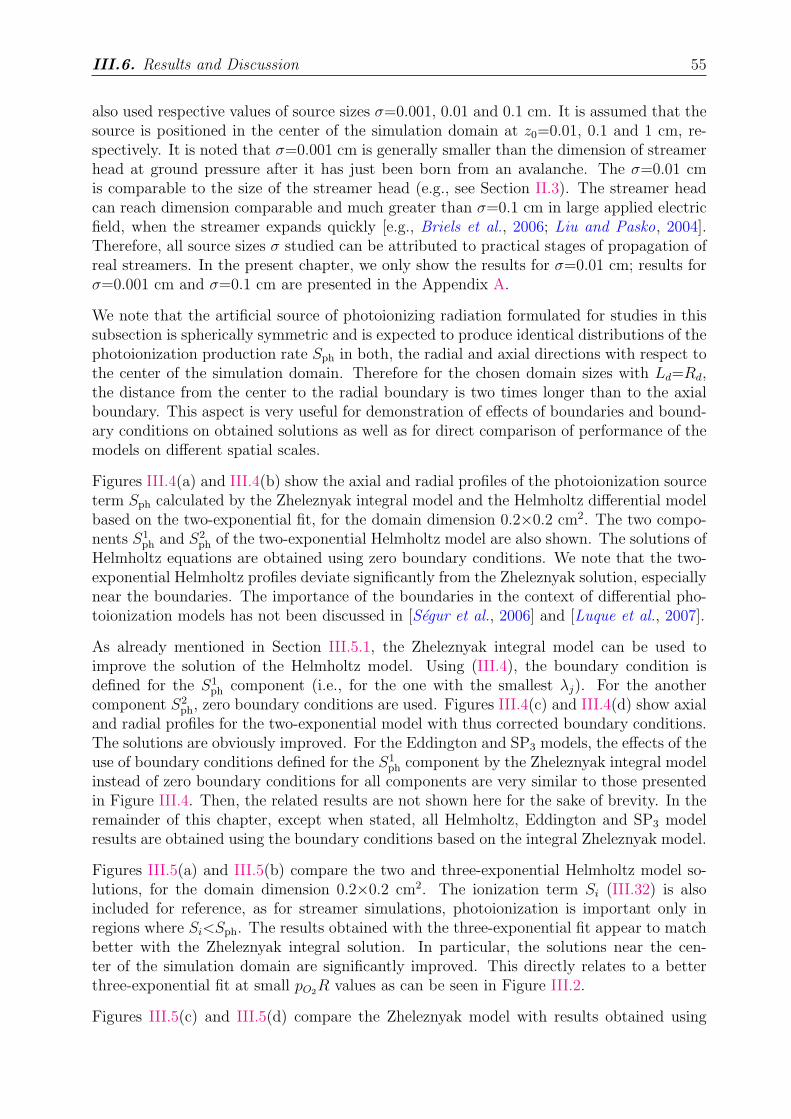
III.6. Results and Discussion 55
also used respective values of source sizes σ=0.001, 0.01 and 0.1 cm. It is assumed that thesource is positioned in the center of the simulation domain at z0=0.01, 0.1 and 1 cm, re-spectively. It is noted that σ=0.001 cm is generally smaller than the dimension of streamerhead at ground pressure after it has just been born from an avalanche. The σ=0.01 cmis comparable to the size of the streamer head (e.g., see Section II.3). The streamer headcan reach dimension comparable and much greater than σ=0.1 cm in large applied electricfield, when the streamer expands quickly [e.g., Briels et al., 2006; Liu and Pasko, 2004].Therefore, all source sizes σ studied can be attributed to practical stages of propagation ofreal streamers. In the present chapter, we only show the results for σ=0.01 cm; results forσ=0.001 cm and σ=0.1 cm are presented in the Appendix A.
We note that the artificial source of photoionizing radiation formulated for studies in thissubsection is spherically symmetric and is expected to produce identical distributions of thephotoionization production rate Sph in both, the radial and axial directions with respect tothe center of the simulation domain. Therefore for the chosen domain sizes with Ld=Rd,the distance from the center to the radial boundary is two times longer than to the axialboundary. This aspect is very useful for demonstration of effects of boundaries and bound-ary conditions on obtained solutions as well as for direct comparison of performance of themodels on different spatial scales.
Figures III.4(a) and III.4(b) show the axial and radial profiles of the photoionization sourceterm Sph calculated by the Zheleznyak integral model and the Helmholtz differential modelbased on the two-exponential fit, for the domain dimension 0.2×0.2 cm2. The two compo-nents S1
ph and S2ph of the two-exponential Helmholtz model are also shown. The solutions of
Helmholtz equations are obtained using zero boundary conditions. We note that the two-exponential Helmholtz profiles deviate significantly from the Zheleznyak solution, especiallynear the boundaries. The importance of the boundaries in the context of differential pho-toionization models has not been discussed in [Ségur et al., 2006] and [Luque et al., 2007].
As already mentioned in Section III.5.1, the Zheleznyak integral model can be used toimprove the solution of the Helmholtz model. Using (III.4), the boundary condition isdefined for the S1
ph component (i.e., for the one with the smallest λj). For the anothercomponent S2
ph, zero boundary conditions are used. Figures III.4(c) and III.4(d) show axialand radial profiles for the two-exponential model with thus corrected boundary conditions.The solutions are obviously improved. For the Eddington and SP3 models, the effects of theuse of boundary conditions defined for the S1
ph component by the Zheleznyak integral modelinstead of zero boundary conditions for all components are very similar to those presentedin Figure III.4. Then, the related results are not shown here for the sake of brevity. In theremainder of this chapter, except when stated, all Helmholtz, Eddington and SP3 modelresults are obtained using the boundary conditions based on the integral Zheleznyak model.
Figures III.5(a) and III.5(b) compare the two and three-exponential Helmholtz model so-lutions, for the domain dimension 0.2×0.2 cm2. The ionization term Si (III.32) is alsoincluded for reference, as for streamer simulations, photoionization is important only inregions where Si<Sph. The results obtained with the three-exponential fit appear to matchbetter with the Zheleznyak integral solution. In particular, the solutions near the cen-ter of the simulation domain are significantly improved. This directly relates to a betterthree-exponential fit at small pO2
R values as can be seen in Figure III.2.
Figures III.5(c) and III.5(d) compare the Zheleznyak model with results obtained using
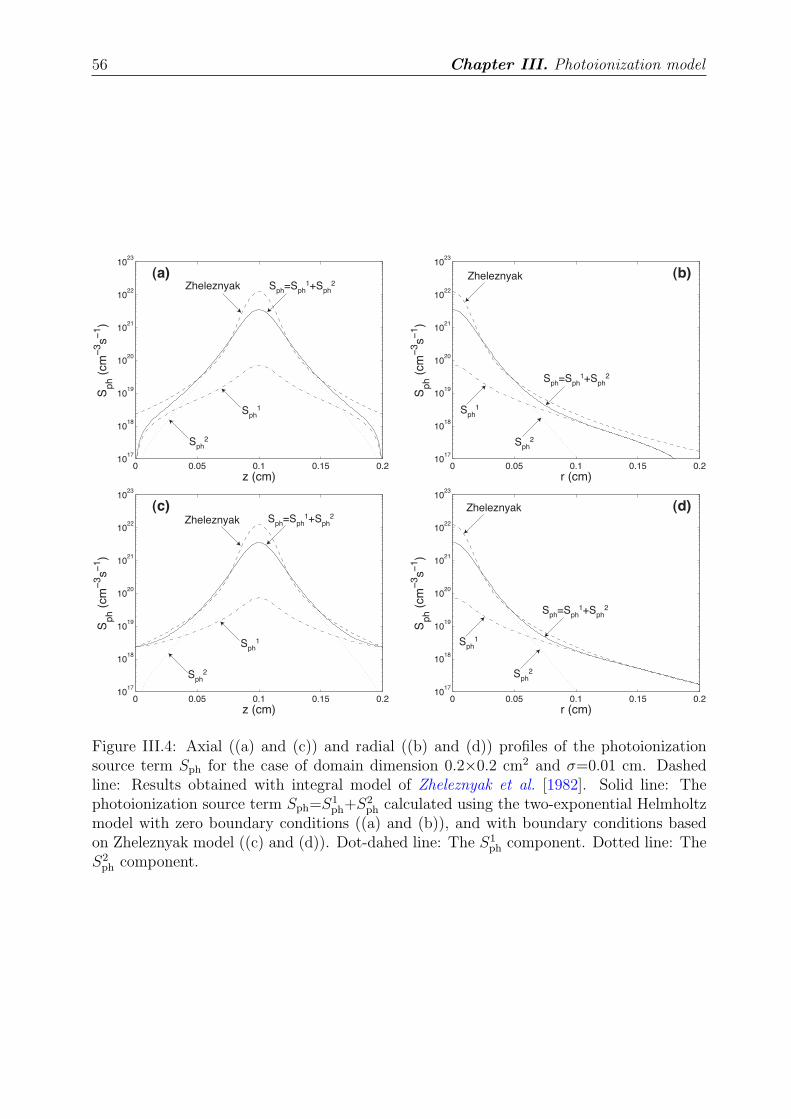
56 Chapter III. Photoionization model
0 0.05 0.1 0.15 0.210
17
1018
1019
1020
1021
1022
1023
z (cm)
Sp
h (
cm
−3s
−1)
(a)
Sph
1
Zheleznyak Sph
=Sph
1+Sph
2
Sph
2
0 0.05 0.1 0.15 0.210
17
1018
1019
1020
1021
1022
1023
r (cm)
Sp
h (
cm
−3s
−1)
(b)
Sph
1
Zheleznyak
Sph
=Sph
1+Sph
2
Sph
2
0 0.05 0.1 0.15 0.210
17
1018
1019
1020
1021
1022
1023
z (cm)
Sp
h (
cm
−3s
−1)
(c)
Sph
1
Zheleznyak Sph
=Sph
1+Sph
2
Sph
2
0 0.05 0.1 0.15 0.210
17
1018
1019
1020
1021
1022
1023
r (cm)
Sp
h (
cm
−3s
−1)
(d)
Sph
1
Zheleznyak
Sph
=Sph
1+Sph
2
Sph
2
Figure III.4: Axial ((a) and (c)) and radial ((b) and (d)) profiles of the photoionizationsource term Sph for the case of domain dimension 0.2×0.2 cm2 and σ=0.01 cm. Dashedline: Results obtained with integral model of Zheleznyak et al. [1982]. Solid line: Thephotoionization source term Sph=S1
ph+S2ph calculated using the two-exponential Helmholtz
model with zero boundary conditions ((a) and (b)), and with boundary conditions basedon Zheleznyak model ((c) and (d)). Dot-dahed line: The S1
ph component. Dotted line: TheS2
ph component.
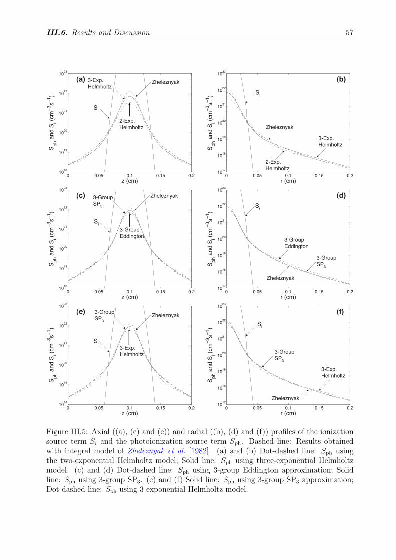
III.6. Results and Discussion 57
0 0.05 0.1 0.15 0.210
18
1019
1020
1021
1022
1023
z (cm)
Sp
h a
nd
Si (
cm
−3s
−1)
(a)
Si
3-Exp.
Helmholtz
2-Exp.
Helmholtz
Zheleznyak
0 0.05 0.1 0.15 0.210
17
1018
1019
1020
1021
1022
1023
r (cm)
Sp
h a
nd
Si (
cm
−3s
−1)
(b)
Si
3-Exp.
Helmholtz
2-Exp.
Helmholtz
Zheleznyak
0 0.05 0.1 0.15 0.210
18
1019
1020
1021
1022
1023
z (cm)
Sp
h a
nd S
i (cm
−3s
−1)
(c)
Si
3-Group
SP3
3-Group
Eddington
Zheleznyak
0 0.05 0.1 0.15 0.210
17
1018
1019
1020
1021
1022
1023
r (cm)
Sp
h a
nd S
i (cm
−3s
−1)
(d)
Si
3-Group
SP3
3-Group
Eddington
Zheleznyak
0 0.05 0.1 0.15 0.210
18
1019
1020
1021
1022
1023
z (cm)
Sp
h a
nd S
i (cm
−3s
−1)
(e)
Si
3-Exp.
Helmholtz
Zheleznyak3-Group
SP3
0 0.05 0.1 0.15 0.210
17
1018
1019
1020
1021
1022
1023
r (cm)
Sp
h a
nd S
i (cm
−3s
−1)
(f)
Si
3-Exp.
Helmholtz
Zheleznyak
3-Group
SP3
Figure III.5: Axial ((a), (c) and (e)) and radial ((b), (d) and (f)) profiles of the ionizationsource term Si and the photoionization source term Sph. Dashed line: Results obtainedwith integral model of Zheleznyak et al. [1982]. (a) and (b) Dot-dashed line: Sph usingthe two-exponential Helmholtz model; Solid line: Sph using three-exponential Helmholtzmodel. (c) and (d) Dot-dashed line: Sph using 3-group Eddington approximation; Solidline: Sph using 3-group SP3. (e) and (f) Solid line: Sph using 3-group SP3 approximation;Dot-dashed line: Sph using 3-exponential Helmholtz model.
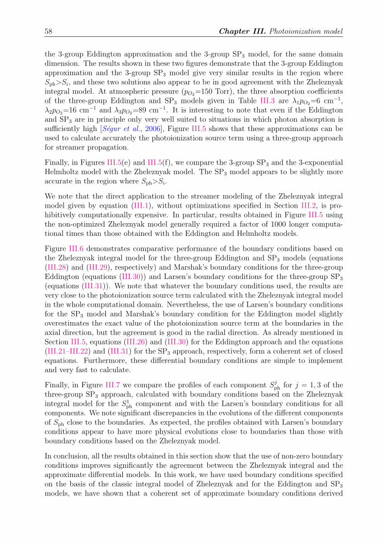
58 Chapter III. Photoionization model
the 3-group Eddington approximation and the 3-group SP3 model, for the same domaindimension. The results shown in these two figures demonstrate that the 3-group Eddingtonapproximation and the 3-group SP3 model give very similar results in the region whereSph>Si, and these two solutions also appear to be in good agreement with the Zheleznyakintegral model. At atmospheric pressure (pO2
=150 Torr), the three absorption coefficientsof the three-group Eddington and SP3 models given in Table III.3 are λ1pO2
=6 cm−1,λ2pO2
=16 cm−1 and λ3pO2=89 cm−1. It is interesting to note that even if the Eddington
and SP3 are in principle only very well suited to situations in which photon absorption issufficiently high [Ségur et al., 2006], Figure III.5 shows that these approximations can beused to calculate accurately the photoionization source term using a three-group approachfor streamer propagation.
Finally, in Figures III.5(e) and III.5(f), we compare the 3-group SP3 and the 3-exponentialHelmholtz model with the Zheleznyak model. The SP3 model appears to be slightly moreaccurate in the region where Sph>Si.
We note that the direct application to the streamer modeling of the Zheleznyak integralmodel given by equation (III.1), without optimizations specified in Section III.2, is pro-hibitively computationally expensive. In particular, results obtained in Figure III.5 usingthe non-optimized Zheleznyak model generally required a factor of 1000 longer computa-tional times than those obtained with the Eddington and Helmholtz models.
Figure III.6 demonstrates comparative performance of the boundary conditions based onthe Zheleznyak integral model for the three-group Eddington and SP3 models (equations(III.28) and (III.29), respectively) and Marshak’s boundary conditions for the three-groupEddington (equations (III.30)) and Larsen’s boundary conditions for the three-group SP3
(equations (III.31)). We note that whatever the boundary conditions used, the results arevery close to the photoionization source term calculated with the Zheleznyak integral modelin the whole computational domain. Nevertheless, the use of Larsen’s boundary conditionsfor the SP3 model and Marshak’s boundary condition for the Eddington model slightlyoverestimates the exact value of the photoionization source term at the boundaries in theaxial direction, but the agreement is good in the radial direction. As already mentioned inSection III.5, equations (III.26) and (III.30) for the Eddington approach and the equations(III.21–III.22) and (III.31) for the SP3 approach, respectively, form a coherent set of closedequations. Furthermore, these differential boundary conditions are simple to implementand very fast to calculate.
Finally, in Figure III.7 we compare the profiles of each component Sjph for j = 1, 3 of the
three-group SP3 approach, calculated with boundary conditions based on the Zheleznyakintegral model for the S1
ph component and with the Larsen’s boundary conditions for allcomponents. We note significant discrepancies in the evolutions of the different componentsof Sph close to the boundaries. As expected, the profiles obtained with Larsen’s boundaryconditions appear to have more physical evolutions close to boundaries than those withboundary conditions based on the Zheleznyak model.
In conclusion, all the results obtained in this section show that the use of non-zero boundaryconditions improves significantly the agreement between the Zheleznyak integral and theapproximate differential models. In this work, we have used boundary conditions specifiedon the basis of the classic integral model of Zheleznyak and for the Eddington and SP3
models, we have shown that a coherent set of approximate boundary conditions derived
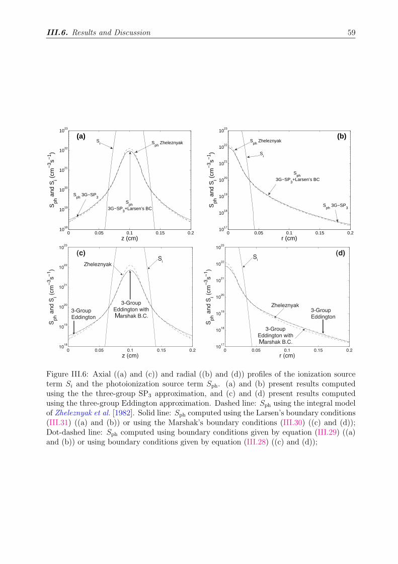
III.6. Results and Discussion 59
0 0.05 0.1 0.15 0.210
18
1019
1020
1021
1022
1023
z (cm)
Sph
and
Si (
cm−
3 s−1 )
(a)S
i Sph
Zheleznyak
Sph
3G−SP
3+Larsen’s BC
Sph
3G−SP3
0 0.05 0.1 0.15 0.210
17
1018
1019
1020
1021
1022
1023
r (cm)
Sph
and
Si (
cm−
3 s−1 )
(b)S
ph Zheleznyak
Si
Sph
3G−SP
3+Larsen’s BC
Sph
3G−SP3
0 0.05 0.1 0.15 0.210
18
1019
1020
1021
1022
1023
z (cm)
Sp
h a
nd S
i (cm
−3s
−1)
(c)S
iZheleznyak
3-Group
Eddington
3-Group
Eddington with
arshak B.C.
0 0.05 0.1 0.15 0.210
17
1018
1019
1020
1021
1022
1023
r (cm)
Sp
h a
nd S
i (cm
−3s
−1)
(d)S
i
Zheleznyak3-Group
Eddington
3-Group
Eddington with
arshak B.C.
M
M
Figure III.6: Axial ((a) and (c)) and radial ((b) and (d)) profiles of the ionization sourceterm Si and the photoionization source term Sph. (a) and (b) present results computedusing the the three-group SP3 approximation, and (c) and (d) present results computedusing the three-group Eddington approximation. Dashed line: Sph using the integral modelof Zheleznyak et al. [1982]. Solid line: Sph computed using the Larsen’s boundary conditions(III.31) ((a) and (b)) or using the Marshak’s boundary conditions (III.30) ((c) and (d));Dot-dashed line: Sph computed using boundary conditions given by equation (III.29) ((a)and (b)) or using boundary conditions given by equation (III.28) ((c) and (d));
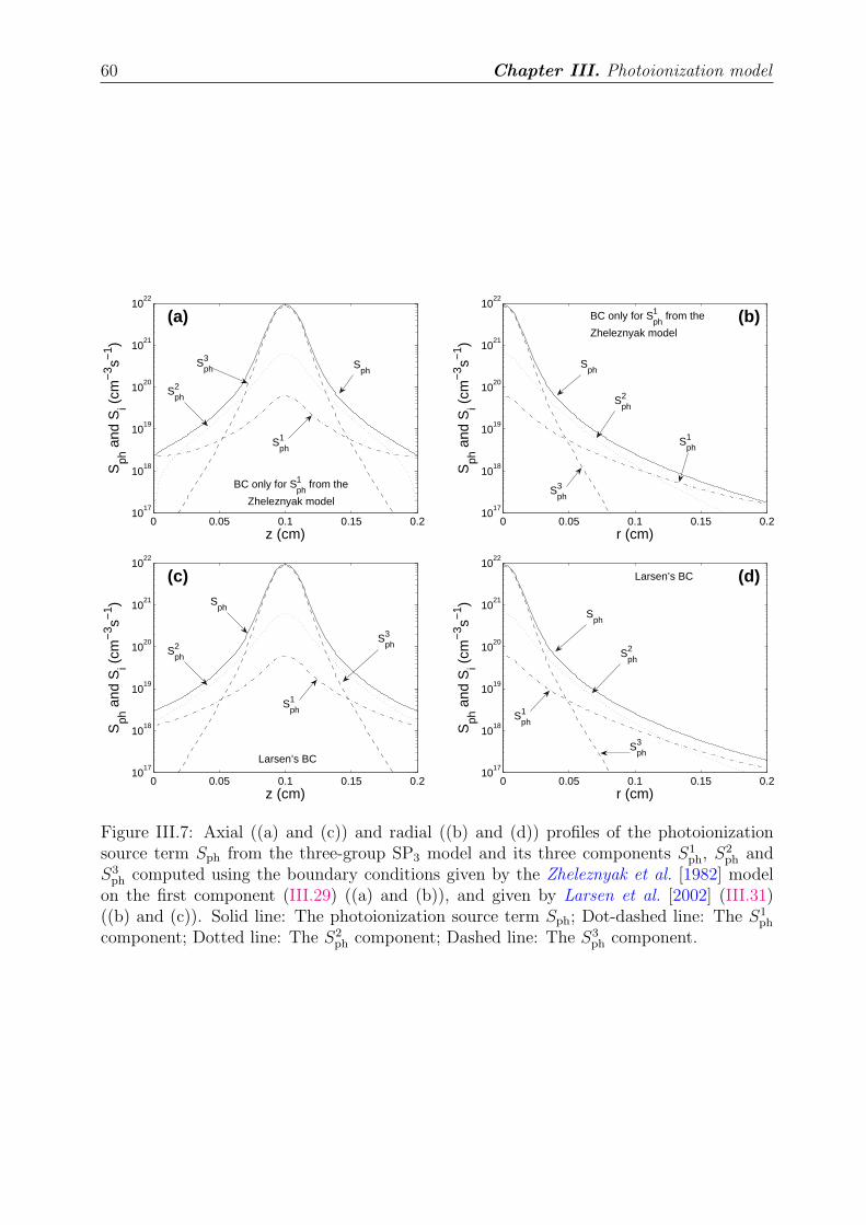
60 Chapter III. Photoionization model
0 0.05 0.1 0.15 0.210
17
1018
1019
1020
1021
1022
z (cm)
Sph
and
Si (
cm−
3 s−1 )
(a)
Sph
Sph3
Sph2
Sph1
BC only for Sph1 from the
Zheleznyak model
0 0.05 0.1 0.15 0.210
17
1018
1019
1020
1021
1022
r (cm)
Sph
and
Si (
cm−
3 s−1 )
(b)
Sph2
Sph1
Sph
Sph3
BC only for Sph1 from the
Zheleznyak model
0 0.05 0.1 0.15 0.210
17
1018
1019
1020
1021
1022
z (cm)
Sph
and
Si (
cm−
3 s−1 )
(c)
Sph3
Sph1
Sph
Sph2
Larsen’s BC
0 0.05 0.1 0.15 0.210
17
1018
1019
1020
1021
1022
r (cm)
Sph
and
Si (
cm−
3 s−1 )
(d)
Sph2
Sph1
Sph3
Sph
Larsen’s BC
Figure III.7: Axial ((a) and (c)) and radial ((b) and (d)) profiles of the photoionizationsource term Sph from the three-group SP3 model and its three components S1
ph, S2ph and
S3ph computed using the boundary conditions given by the Zheleznyak et al. [1982] model
on the first component (III.29) ((a) and (b)), and given by Larsen et al. [2002] (III.31)((b) and (c)). Solid line: The photoionization source term Sph; Dot-dashed line: The S1
ph
component; Dotted line: The S2ph component; Dashed line: The S3
ph component.
III.6. Results and Discussion 61
from radiation transfer theory can be successfully used. We have also shown that the useof a three-exponential fit either with the SP3 model or with the Helmholtz model allows toobtain a good agreement with the Zheleznyak integral model, and that the two-exponentialfit is generally not sufficient to reproduce the Zheleznyak model accurately for the fullrange of validity of this model (i.e., up to pO2
R≃100 Torr cm, or R≃0.7 cm at groundpressure [Naidis , 2006]; see Appendix A). It is interesting to note also that although theEddington and SP3 are in principle only very well suited to situations in which photonabsorption is sufficiently high, these approximations can be used to calculate accuratelythe photoionization source term using a three-group approach for streamer propagation.The models derived in this chapter are only slightly more complicated than the one-groupmodel proposed in [Ségur et al., 2006], but remain simple to implement in streamer codes.Results of the practical application of these models to streamer problems are presentedin the next section, in which we also discuss computational expenses involved in differenttypes of photoionization models.
III.6.2 Streamer simulations
In this section, the three-exponential Helmholtz, and the three-group Eddington and SP3
differential photoionization models are used for two realistic problems:
• the development of a double-headed streamer in a high electric field (>Ek) at groundpressure,
• the streamer propagation in weak external electric fields (<Ek) at ground pressure.
The validity and range of applicability of the developed models for the photoionizationterm is demonstrated by performing direct comparisons of the results from these modelsand results obtained from the classic integral model of Zheleznyak et al. [1982].
In this work we use the drift-diffusion equations of the streamer fluid model (I.28)-(I.30)coupled to Poisson’s equation (I.31). On timescales of interest for studies presented in thischapter, ions are assumed to be motionless. For test studies presented in this chapter alltransport parameters and reaction rates in air are taken from [Morrow and Lowke, 1997].Axisymmetric streamers are studied and thus cylindrical coordinates introduced in SectionIII.2 are used.
In this section, two sets of numerical techniques are used for solving the streamer modelequations:
1. The charged species transport equations are solved using a flux-corrected transport(FCT) method (see paragraph “FCT method” in Section II.2.2). The 3rd orderQUICKEST scheme is used as the high order scheme and an upwind scheme for thelow order scheme. The flux limiter derived by Zalesak [1979] is adopted for thisFCT method. The finite difference form of the Poisson’s equation is solved using theD03EBF module of the NAG Fortran library (http://www.nag.co.uk).
2. The charged species transport equations are solved using a modified Scharfetter-Gummel (SG) algorithm (see paragraph “Modified SG scheme” in Section II.2.2),and the finite difference form of Poisson’s equation is solved by successive overrelax-ation (SOR) method [see Liu and Pasko, 2004, and references cited therein].
62 Chapter III. Photoionization model
It is interesting to note that we have also carried out some streamer simulations using the di-rect solver SuperLU [Demmel et al., 1999a, b] (http://crd.lbl.gov/~xiaoye/SuperLU/)to solve the Poisson’s equation. The results obtained have been found to be very close tothose given by iterative solvers.
The boundary conditions for the potential required for the solution of the Poisson’s equationare obtained using integral solutions of the Poisson’s equation, which accounts for the knowncharge distribution inside of the simulation domain (see Section II.1.2). As stated in SectionII.1.2, the applied technique allows to use a relatively small simulation domain in transverse(i.e., radial) direction to obtain an accurate solution for the electric potential.
The calculation of the boundary conditions in streamer simulations can be significantlyaccelerated since only a small number of grids inside of the simulation domain (usuallyaround streamer body and streamer head(s)) possesses charge density values significantlycontributing to the potential values at the boundary. In practical calculations the simula-tion domain is scanned to find the maximum magnitude of the charge density value |ρmax|,and it has been verified by separate tests that accounting only for grids with charge densitymagnitudes, which exceed 0.1% of this value (i.e., |ρ|>0.001 |ρmax|) leads to fast, accurateand robust evaluation of boundary conditions for potential, allowing effective use of simu-lation domains with very small size in radial direction. Further improvements in terms ofexecution speed can be achieved due to a relatively smooth spatial variation of the potentialat the boundaries. The potential can be evaluated at a selected set of points and interpola-tion can be used to obtain the values at all grid points constituting the boundary. Due to avery small time step used in streamer modeling (usually defined by the ionization time scaleassociated with the large electric field in the streamer head as already mentioned above)it is also possible, especially for preliminary test runs, to evaluate boundary conditionsonly once during several steps of the model execution. However, for all streamer resultspresented in this section the update of potential boundary conditions has been performedat every time step for maximum accuracy of results.
For photoionization calculations in the streamer model we employ techniques discussedin Sections III.2, III.3 and III.4. Specifically, for the present study we have implementedthe three-group Eddington and SP3, the three-exponential Helmholtz, and the classicalintegral models. The quenching pressure is assumed to be pq = 30 Torr, and the ratioξνu/νi, appearing in (III.2), is assumed to depend on the reduced electric field as specifiedin [Liu and Pasko, 2004]. The finite difference forms of the Eddington, SP3 and Helmholtzphotoionization model equations are solved using the same module of the NAG Fortranlibrary used for the solution of the Poisson’s equation. It is interesting to note that wehave also carried out tests using the direct solver SuperLU (see Section II.1.3) for thecomputation of the photoionization source term based on the Eddington and SP3 models.The results have been found to be very close to those obtained using the iterative solvers.The three differential models for photoionization are implemented within the context ofthe first set of numerical techniques described above (i.e., the FCT based). Within thecontext of the second set of numerical techniques (i.e., the SG based), we implemented theclassical integral and the Helmholtz models. The finite difference equations of the Helmholtzphotoionization model are solved by the SOR method for this case. The modeling resultsobtained by using different numerical techniques to solve the Helmholtz model equationsare very similar and we will not differentiate them in the following sections of this chapter.
III.6. Results and Discussion 63
Double-headed streamers in air
In this section, we report and compare modeling results on a double-headed streamer de-veloping in air at ground pressure (760 Torr) obtained with the different photoionizationmodels discussed in this chapter. The simulation domain is the same as in [Liu and Pasko,2004, Figure 4a]. Two remote electrodes with a certain potential difference establish auniform Laplacian field E0=4.8×10⁶ V/m. All results are obtained assuming air neutraldensity N0=2.688×1025 m−3, and therefore E0/N0=178.6 Td (1 Td=10−17 V cm2). Un-der the influence of this applied field, a double-headed streamer is launched by placing aneutral plasma cloud in the simulation domain. The initial plasma cloud has a Gaussiandistribution in space:
ne(r, z)|t=0 = np(r, z)|t=0 = n0 exp
[
−(
r
σr
)2
−(
z − z0
σz
)2]
. (III.34)
The center of the Gaussian distribution is located in the middle of the simulation domain,at z0=0.7 cm, and it is assumed that σr=σz=0.02 cm and n0=1020 m−3. The size of thecomputational domain is 1.4 × 0.125 cm2. The computational grid is uniform in bothradial and axial directions. The total number of cells is nz×nr=1681×151, where nz andnr represent number of cells in the axial and radial directions, respectively. As part ofpreparatory work for the model studies presented in this chapter we have conducted severaltest runs with 2400×100 grid points with a refined mesh in the radial direction and uniformmesh in the axial direction. Results appeared to be identical to those obtained with the1681×151 uniform mesh, which therefore was adopted for all runs presented in this section.
Concerning the photoionization source term, it has been verified by practical tests thatvery accurate results for the photoionization production rate can be obtained even if thephotoionization is calculated once during every ten steps of the execution of the streamermodel. This approach is justified due to the very small time step used in the streamermodeling. Additionally, for photoionization calculations the Sph term is usually negligiblein the immediate vicinity of the streamer head due to the domination of the ionizationterm Si, and electrons created by photoionization well ahead of the streamer head gothrough a relatively long (in comparison with the model time step) evolution and avalanchemultiplication before they affect the dynamics of the streamer head.
Before the incorporation of different photoionization models, we tested the performanceof the two sets of numerical techniques described in Sections II.2.2 and II.2.2 (i.e., theFCT and SG based) using a double-headed streamer test case for which photoionizationeffects are not included and the pre-ionization level is only supplied by a uniform neutralbackground plasma with initial density of 1014 m−3. This approach is similar to the oneapplied in a classic paper of Dhali and Williams [1987]. Only very small differences areobserved in results obtained with the two models for the modeled double-headed streamer.Specifically, by the time moment 3.5 ns from the beginning of the model execution thedifferences between the peak electron number densities and peak electric fields between twomodel streamers do not exceed 7.8% and 2.6%, respectively. It is noted that these differ-ences do not exceed those arising from known limitations of the local field approximationin streamer modeling [Naidis , 1997; Li et al., 2007] (see Section I.3.5). The test resultsconcerning the double-headed streamer are not shown in this thesis for the sake of brevity,but essentially the same agreement between the two numerical techniques can be observed
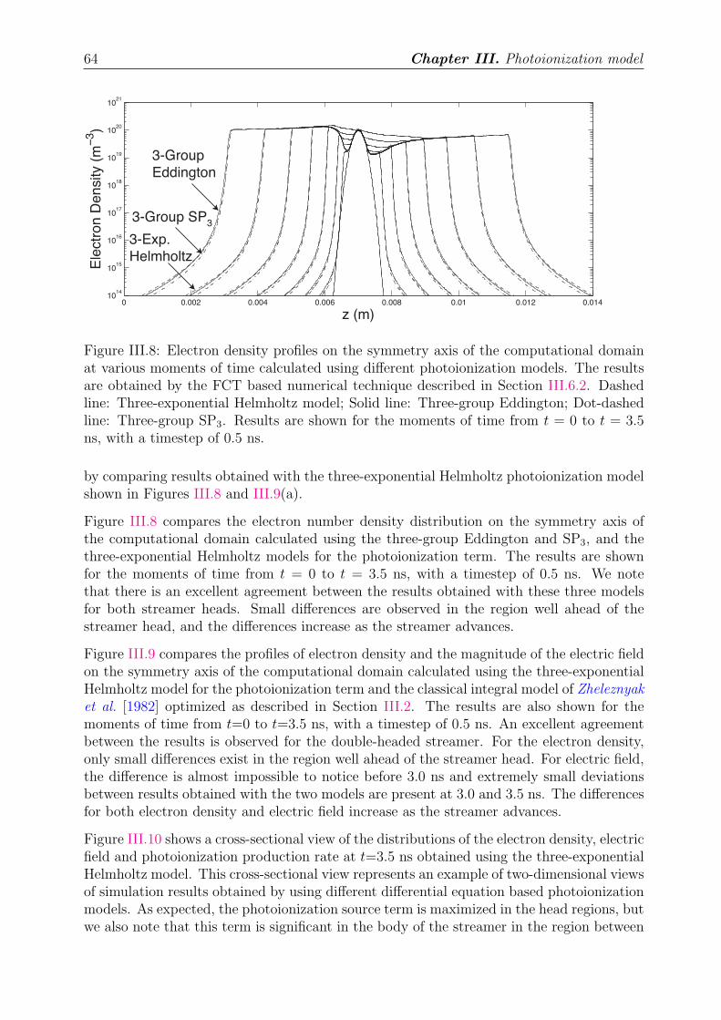
64 Chapter III. Photoionization model
0 0.002 0.004 0.006 0.008 0.01 0.012 0.01410
14
1015
1016
1017
1018
1019
1020
1021
z (m)
Ele
ctr
on
De
nsity (
m−
3)
3-Exp.
Helmholtz
3-Group
Eddington
3-Group SP3
Figure III.8: Electron density profiles on the symmetry axis of the computational domainat various moments of time calculated using different photoionization models. The resultsare obtained by the FCT based numerical technique described in Section III.6.2. Dashedline: Three-exponential Helmholtz model; Solid line: Three-group Eddington; Dot-dashedline: Three-group SP3. Results are shown for the moments of time from t = 0 to t = 3.5ns, with a timestep of 0.5 ns.
by comparing results obtained with the three-exponential Helmholtz photoionization modelshown in Figures III.8 and III.9(a).
Figure III.8 compares the electron number density distribution on the symmetry axis ofthe computational domain calculated using the three-group Eddington and SP3, and thethree-exponential Helmholtz models for the photoionization term. The results are shownfor the moments of time from t = 0 to t = 3.5 ns, with a timestep of 0.5 ns. We notethat there is an excellent agreement between the results obtained with these three modelsfor both streamer heads. Small differences are observed in the region well ahead of thestreamer head, and the differences increase as the streamer advances.
Figure III.9 compares the profiles of electron density and the magnitude of the electric fieldon the symmetry axis of the computational domain calculated using the three-exponentialHelmholtz model for the photoionization term and the classical integral model of Zheleznyaket al. [1982] optimized as described in Section III.2. The results are also shown for themoments of time from t=0 to t=3.5 ns, with a timestep of 0.5 ns. An excellent agreementbetween the results is observed for the double-headed streamer. For the electron density,only small differences exist in the region well ahead of the streamer head. For electric field,the difference is almost impossible to notice before 3.0 ns and extremely small deviationsbetween results obtained with the two models are present at 3.0 and 3.5 ns. The differencesfor both electron density and electric field increase as the streamer advances.
Figure III.10 shows a cross-sectional view of the distributions of the electron density, electricfield and photoionization production rate at t=3.5 ns obtained using the three-exponentialHelmholtz model. This cross-sectional view represents an example of two-dimensional viewsof simulation results obtained by using different differential equation based photoionizationmodels. As expected, the photoionization source term is maximized in the head regions, butwe also note that this term is significant in the body of the streamer in the region between
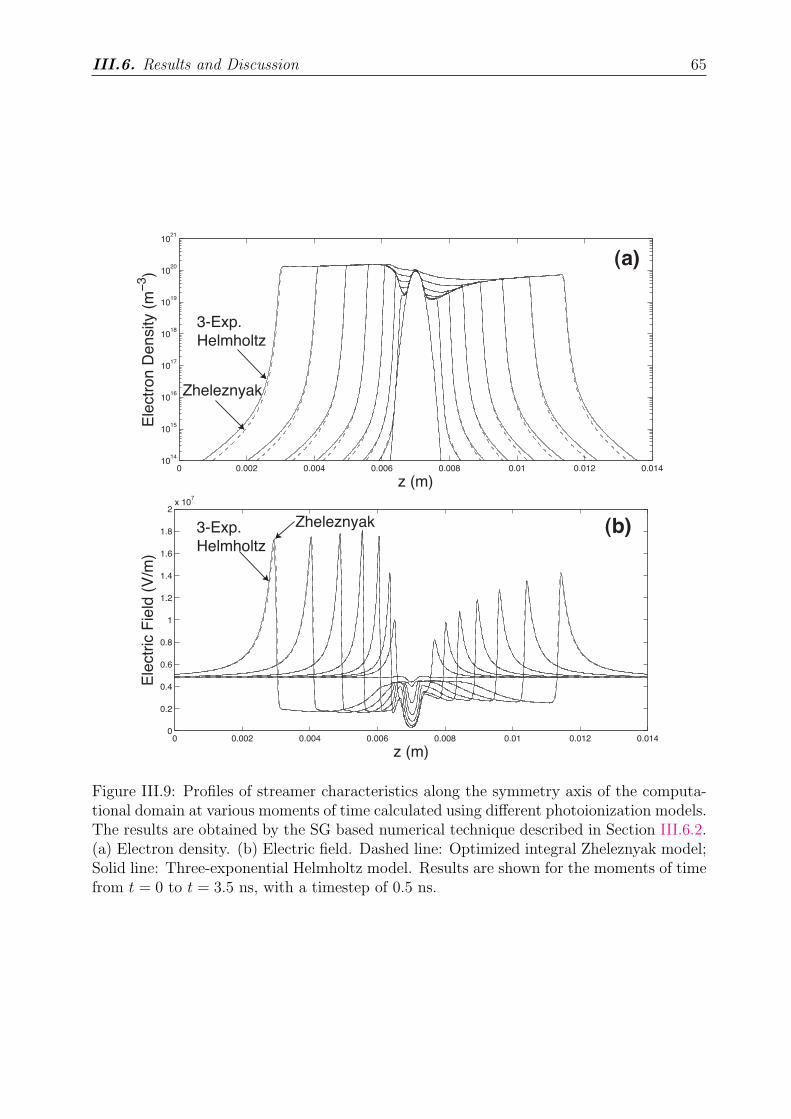
III.6. Results and Discussion 65
0 0.002 0.004 0.006 0.008 0.01 0.012 0.01410
14
1015
1016
1017
1018
1019
1020
1021
z (m)
Ele
ctr
on
De
nsity (
m−
3)
3-Exp.
Helmholtz
Zheleznyak
(a)
0 0.002 0.004 0.006 0.008 0.01 0.012 0.0140
0.2
0.4
0.6
0.8
1
1.2
1.4
1.6
1.8
2x 10
7
z (m)
Ele
ctr
ic F
ield
(V
/m)
3-Exp.
Helmholtz
Zheleznyak (b)
Figure III.9: Profiles of streamer characteristics along the symmetry axis of the computa-tional domain at various moments of time calculated using different photoionization models.The results are obtained by the SG based numerical technique described in Section III.6.2.(a) Electron density. (b) Electric field. Dashed line: Optimized integral Zheleznyak model;Solid line: Three-exponential Helmholtz model. Results are shown for the moments of timefrom t = 0 to t = 3.5 ns, with a timestep of 0.5 ns.
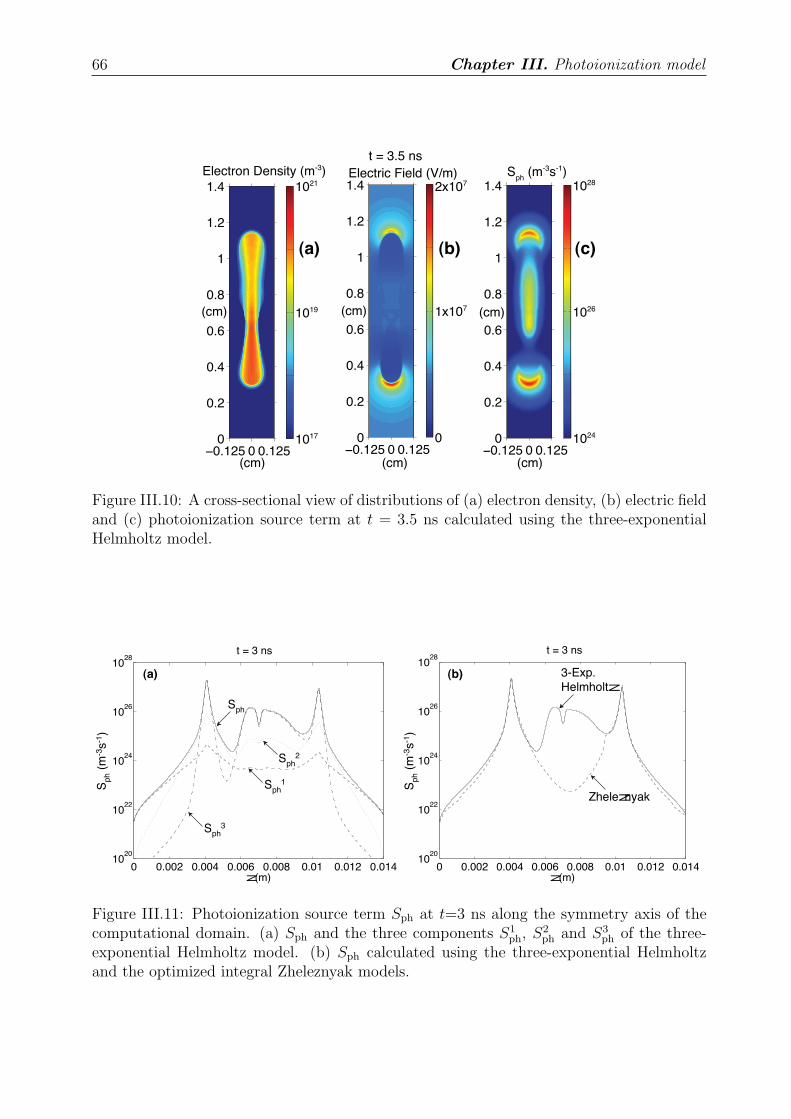
66 Chapter III. Photoionization model
t = 3.5 nsElectron Density (m-3)
(cm)
(cm)
−0.125 0 0.125
1.4
1.2
1
0.8
0.6
0.4
0.2
0 1017
1019
1021Electric Field (V/m)
(cm)
(cm)
−0.125 0 0.125
1.4
1.2
1
0.8
0.6
0.4
0.2
0 0
1x10⁷
2x10⁷S
ph (m-3s-1)
(cm)
(cm)
−0.125 0 0.125
1.4
1.2
1
0.8
0.6
0.4
0.2
0 1024
1026
1028
(a) (b) (c)
Figure III.10: A cross-sectional view of distributions of (a) electron density, (b) electric fieldand (c) photoionization source term at t = 3.5 ns calculated using the three-exponentialHelmholtz model.
0 0.002 0.004 0.006 0.008 0.01 0.012 0.01410
20
1022
1024
1026
1028
z (m)
Sph (
m-3
s-1
)
Sph (
m-3
s-1
)
t = 3 ns
3-Exp.
Helmholtz
Zheleznyak
(b)
0 0.002 0.004 0.006 0.008 0.01 0.012 0.01410
20
1022
1024
1026
1028
z (m)
t = 3 ns
(a)
Sph
3
Sph
1
Sph
Sph
2
Figure III.11: Photoionization source term Sph at t=3 ns along the symmetry axis of thecomputational domain. (a) Sph and the three components S1
ph, S2ph and S3
ph of the three-exponential Helmholtz model. (b) Sph calculated using the three-exponential Helmholtzand the optimized integral Zheleznyak models.
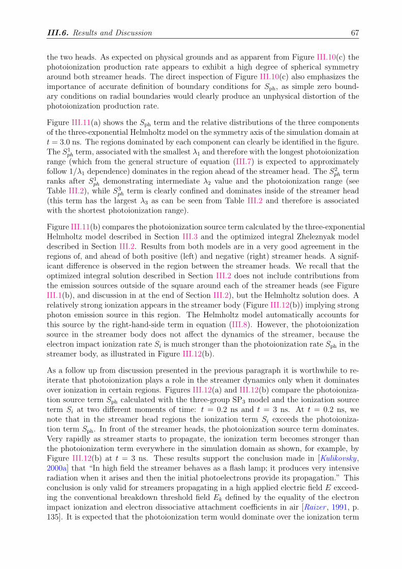
III.6. Results and Discussion 67
the two heads. As expected on physical grounds and as apparent from Figure III.10(c) thephotoionization production rate appears to exhibit a high degree of spherical symmetryaround both streamer heads. The direct inspection of Figure III.10(c) also emphasizes theimportance of accurate definition of boundary conditions for Sph, as simple zero bound-ary conditions on radial boundaries would clearly produce an unphysical distortion of thephotoionization production rate.
Figure III.11(a) shows the Sph term and the relative distributions of the three componentsof the three-exponential Helmholtz model on the symmetry axis of the simulation domain att = 3.0 ns. The regions dominated by each component can clearly be identified in the figure.The S1
ph term, associated with the smallest λ1 and therefore with the longest photoionizationrange (which from the general structure of equation (III.7) is expected to approximatelyfollow 1/λ1 dependence) dominates in the region ahead of the streamer head. The S2
ph termranks after S1
ph demonstrating intermediate λ2 value and the photoionization range (seeTable III.2), while S3
ph term is clearly confined and dominates inside of the streamer head(this term has the largest λ3 as can be seen from Table III.2 and therefore is associatedwith the shortest photoionization range).
Figure III.11(b) compares the photoionization source term calculated by the three-exponentialHelmholtz model described in Section III.3 and the optimized integral Zheleznyak modeldescribed in Section III.2. Results from both models are in a very good agreement in theregions of, and ahead of both positive (left) and negative (right) streamer heads. A signif-icant difference is observed in the region between the streamer heads. We recall that theoptimized integral solution described in Section III.2 does not include contributions fromthe emission sources outside of the square around each of the streamer heads (see FigureIII.1(b), and discussion in at the end of Section III.2), but the Helmholtz solution does. Arelatively strong ionization appears in the streamer body (Figure III.12(b)) implying strongphoton emission source in this region. The Helmholtz model automatically accounts forthis source by the right-hand-side term in equation (III.8). However, the photoionizationsource in the streamer body does not affect the dynamics of the streamer, because theelectron impact ionization rate Si is much stronger than the photoionization rate Sph in thestreamer body, as illustrated in Figure III.12(b).
As a follow up from discussion presented in the previous paragraph it is worthwhile to re-iterate that photoionization plays a role in the streamer dynamics only when it dominatesover ionization in certain regions. Figures III.12(a) and III.12(b) compare the photoioniza-tion source term Sph calculated with the three-group SP3 model and the ionization sourceterm Si at two different moments of time: t = 0.2 ns and t = 3 ns. At t = 0.2 ns, wenote that in the streamer head regions the ionization term Si exceeds the photoioniza-tion term Sph. In front of the streamer heads, the photoionization source term dominates.Very rapidly as streamer starts to propagate, the ionization term becomes stronger thanthe photoionization term everywhere in the simulation domain as shown, for example, byFigure III.12(b) at t = 3 ns. These results support the conclusion made in [Kulikovsky ,2000a] that “In high field the streamer behaves as a flash lamp; it produces very intensiveradiation when it arises and then the initial photoelectrons provide its propagation.” Thisconclusion is only valid for streamers propagating in a high applied electric field E exceed-ing the conventional breakdown threshold field Ek defined by the equality of the electronimpact ionization and electron dissociative attachment coefficients in air [Raizer , 1991, p.135]. It is expected that the photoionization term would dominate over the ionization term
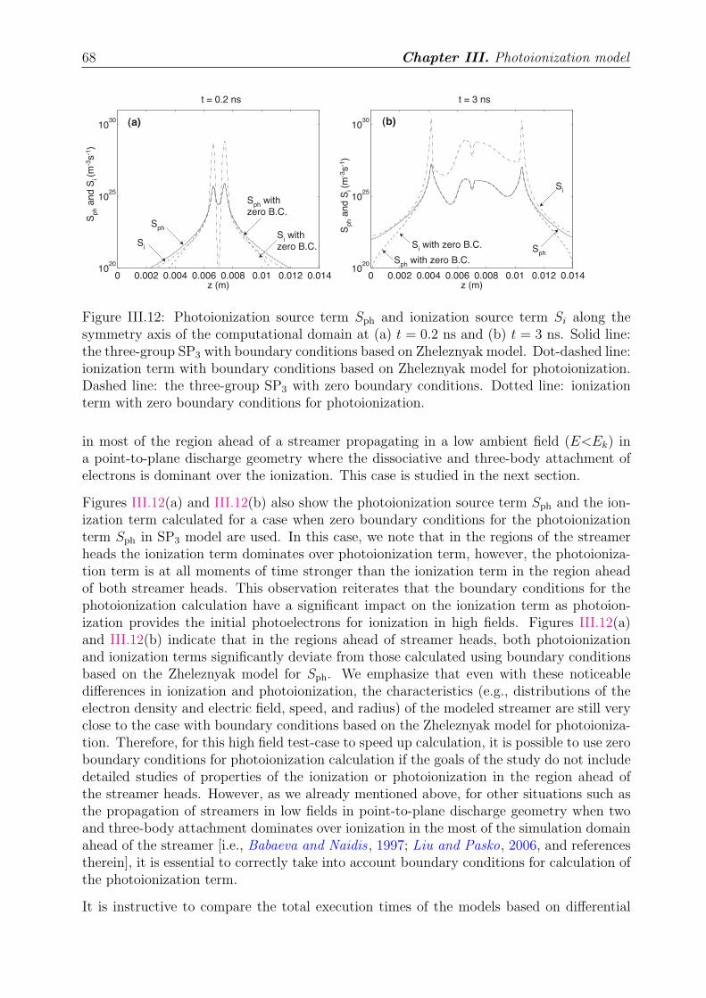
68 Chapter III. Photoionization model
0 0.002 0.004 0.006 0.008 0.01 0.012 0.01410
20
1025
1030
z (m)
t = 0.2 ns
Si
Sph
Sph
with
zero B.C.
Sph a
nd S
i (m
-3s
-1)
Si with
zero B.C.
(a)
0 0.002 0.004 0.006 0.008 0.01 0.012 0.01410
20
1025
1030
z (m)
t = 3 ns
Si
Sph
Sph
with zero B.C.
Si with zero B.C.
Sph a
nd S
i (m
-3s
-1)
(b)
Figure III.12: Photoionization source term Sph and ionization source term Si along thesymmetry axis of the computational domain at (a) t = 0.2 ns and (b) t = 3 ns. Solid line:the three-group SP3 with boundary conditions based on Zheleznyak model. Dot-dashed line:ionization term with boundary conditions based on Zheleznyak model for photoionization.Dashed line: the three-group SP3 with zero boundary conditions. Dotted line: ionizationterm with zero boundary conditions for photoionization.
in most of the region ahead of a streamer propagating in a low ambient field (E<Ek) ina point-to-plane discharge geometry where the dissociative and three-body attachment ofelectrons is dominant over the ionization. This case is studied in the next section.
Figures III.12(a) and III.12(b) also show the photoionization source term Sph and the ion-ization term calculated for a case when zero boundary conditions for the photoionizationterm Sph in SP3 model are used. In this case, we note that in the regions of the streamerheads the ionization term dominates over photoionization term, however, the photoioniza-tion term is at all moments of time stronger than the ionization term in the region aheadof both streamer heads. This observation reiterates that the boundary conditions for thephotoionization calculation have a significant impact on the ionization term as photoion-ization provides the initial photoelectrons for ionization in high fields. Figures III.12(a)and III.12(b) indicate that in the regions ahead of streamer heads, both photoionizationand ionization terms significantly deviate from those calculated using boundary conditionsbased on the Zheleznyak model for Sph. We emphasize that even with these noticeabledifferences in ionization and photoionization, the characteristics (e.g., distributions of theelectron density and electric field, speed, and radius) of the modeled streamer are still veryclose to the case with boundary conditions based on the Zheleznyak model for photoioniza-tion. Therefore, for this high field test-case to speed up calculation, it is possible to use zeroboundary conditions for photoionization calculation if the goals of the study do not includedetailed studies of properties of the ionization or photoionization in the region ahead ofthe streamer heads. However, as we already mentioned above, for other situations such asthe propagation of streamers in low fields in point-to-plane discharge geometry when twoand three-body attachment dominates over ionization in the most of the simulation domainahead of the streamer [i.e., Babaeva and Naidis , 1997; Liu and Pasko, 2006, and referencestherein], it is essential to correctly take into account boundary conditions for calculation ofthe photoionization term.
It is instructive to compare the total execution times of the models based on differential
III.6. Results and Discussion 69
equation approach in comparison with the optimized integral Zheleznyak model. We havenoticed that the simulation time of the three-group Eddington approach with boundaryconditions given by equation (III.28) is similar to the one of the three-exponential Helmholtzmodel with boundary conditions based on Zheleznyak model given in Section III.3, whereasthe simulation time of the three-group SP3 with boundary conditions given by equation(III.29) is slightly longer. As an example of such comparisons we conducted accuratemeasurements of computation times involved in two model cases shown in Figure III.9.We reiterate that both models are executed on the same hardware (2 GHz Power MacG5 running Mac OS X 10.4) with identical grids and algorithms to define time steps andboundary conditions. As already mentioned, the photoionization production rate has beenupdated after every ten steps of the model execution and the boundary conditions for theelectric potential have been updated every time step. The measured total execution timeof the code based on the optimized implementation of the Zheleznyak et al. [1982] integralphotoionization model as described in Section III.2 was 53 hours and 20 minutes. Themeasured execution time of the code based on the three-exponential Helmholtz model withboundary conditions based on Zheleznyak model described in Section III.3 was 63 hoursand 14 minutes. The time profiling indicates that about 80% of the model execution time isspent in both cases on updates of the boundary conditions for the potential and the solutionof the Poisson equation for the electric field. It is noted that even if the photoionizationproduction rate is updated at every time step, the execution times of both models will beof the same order.
The difference in the computation time presented above may seem in favor to the integralphotoionization model, however, it is important to point out that the optimization (intro-duction of moving meshes with variable cell sizes and employment of effective windowingand interpolation techniques) of the integral model is rather involved and complex, and re-quires a separate adaptation effort to extend it to every new configuration studied. At thesame time, the implementation of the photoionization models based on differential equationapproach is straightforward and simple. Furthermore, in the optimized integral approachthe photoionization source term is calculated accurately only close the the streamer heads.For example, in the double-headed test-case, we have shown that due to the optimization,in the region between the streamer heads, the photoionization source term is not calcu-lated accurately using the integral model. Conversely with the differential approaches thephotoionization term is calculated accurately in the whole computation domain.
Propagation of streamer in a weak external field
In the present section, we apply the three-exponential Helmholtz and three-group SP3
models to the simulation of streamers propagating in weak external electric fields (<Ek, seeI.1.3), which is a configuration where photoionization has a much more significant impacton the streamer dynamics than in the high-field case studied previously. Moreover this weakfield condition is of great interest for many practical applications of streamers. We proposeto validate the three-exponential Helmholtz and three-group SP3 models by comparing thecorresponding results with those obtained with the Zheleznyak model. The objective of thiswork is to demonstrate the validity and accuracy of the three-exponential Helmholtz andthree-group SP3 models for studies of streamer discharges in air for a wide range of appliedelectric fields.
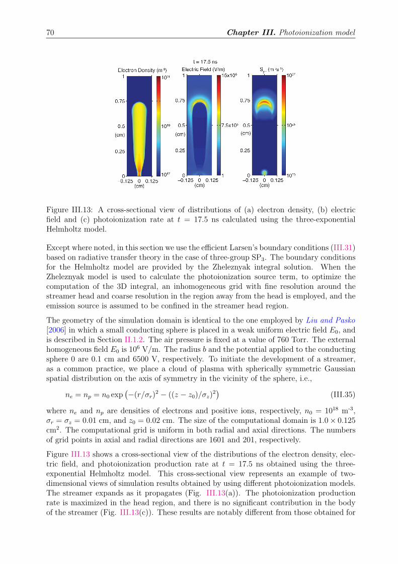
70 Chapter III. Photoionization model
Figure III.13: A cross-sectional view of distributions of (a) electron density, (b) electricfield and (c) photoionization rate at t = 17.5 ns calculated using the three-exponentialHelmholtz model.
Except where noted, in this section we use the efficient Larsen’s boundary conditions (III.31)based on radiative transfer theory in the case of three-group SP3. The boundary conditionsfor the Helmholtz model are provided by the Zheleznyak integral solution. When theZheleznyak model is used to calculate the photoionization source term, to optimize thecomputation of the 3D integral, an inhomogeneous grid with fine resolution around thestreamer head and coarse resolution in the region away from the head is employed, and theemission source is assumed to be confined in the streamer head region.
The geometry of the simulation domain is identical to the one employed by Liu and Pasko[2006] in which a small conducting sphere is placed in a weak uniform electric field E0, andis described in Section II.1.2. The air pressure is fixed at a value of 760 Torr. The externalhomogeneous field E0 is 106 V/m. The radius b and the potential applied to the conductingsphere 0 are 0.1 cm and 6500 V, respectively. To initiate the development of a streamer,as a common practice, we place a cloud of plasma with spherically symmetric Gaussianspatial distribution on the axis of symmetry in the vicinity of the sphere, i.e.,
ne = np = n0 exp(
−(r/σr)2 − ((z − z0)/σz)
2)
(III.35)
where ne and np are densities of electrons and positive ions, respectively, n0 = 1018 m-3,σr = σz = 0.01 cm, and z0 = 0.02 cm. The size of the computational domain is 1.0× 0.125cm2. The computational grid is uniform in both radial and axial directions. The numbersof grid points in axial and radial directions are 1601 and 201, respectively.
Figure III.13 shows a cross-sectional view of the distributions of the electron density, elec-tric field, and photoionization production rate at t = 17.5 ns obtained using the three-exponential Helmholtz model. This cross-sectional view represents an example of two-dimensional views of simulation results obtained by using different photoionization models.The streamer expands as it propagates (Fig. III.13(a)). The photoionization productionrate is maximized in the head region, and there is no significant contribution in the bodyof the streamer (Fig. III.13(c)). These results are notably different from those obtained for
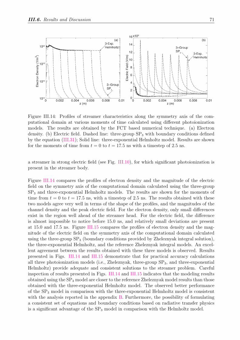
III.6. Results and Discussion 71
Figure III.14: Profiles of streamer characteristics along the symmetry axis of the com-putational domain at various moments of time calculated using different photoionizationmodels. The results are obtained by the FCT based numerical technique. (a) Electrondensity. (b) Electric field. Dashed line: three-group SP3 with boundary conditions definedby the equation (III.31); Solid line: three-exponential Helmholtz model. Results are shownfor the moments of time from t = 0 to t = 17.5 ns with a timestep of 2.5 ns.
a streamer in strong electric field (see Fig. III.10), for which significant photoionization ispresent in the streamer body.
Figure III.14 compares the profiles of electron density and the magnitude of the electricfield on the symmetry axis of the computational domain calculated using the three-groupSP3 and three-exponential Helmholtz models. The results are shown for the moments oftime from t = 0 to t = 17.5 ns, with a timestep of 2.5 ns. The results obtained with thesetwo models agree very well in terms of the shape of the profiles, and the magnitudes of thechannel density and the peak electric field. For the electron density, only small differencesexist in the region well ahead of the streamer head. For the electric field, the differenceis almost impossible to notice before 15.0 ns, and relatively small deviations are presentat 15.0 and 17.5 ns. Figure III.15 compares the profiles of electron density and the mag-nitude of the electric field on the symmetry axis of the computational domain calculatedusing the three-group SP3 (boundary conditions provided by Zheleznyak integral solution),the three-exponential Helmholtz, and the reference Zheleznyak integral models. An excel-lent agreement between the results obtained with these three models is observed. Resultspresented in Figs. III.14 and III.15 demonstrate that for practical accuracy calculationsall three photoionization models (i.e., Zheleznyak, three-group SP3, and three-exponentialHelmholtz) provide adequate and consistent solutions to the streamer problem. Carefulinspection of results presented in Figs. III.14 and III.15 indicates that the modeling resultsobtained using the SP3 model are closer to the reference Zheleznyak model results than thoseobtained with the three-exponential Helmholtz model. The observed better performanceof the SP3 model in comparison with the three-exponential Helmholtz model is consistentwith the analysis reported in the appendix B. Furthermore, the possibility of formulatinga consistent set of equations and boundary conditions based on radiative transfer physicsis a significant advantage of the SP3 model in comparison with the Helmholtz model.
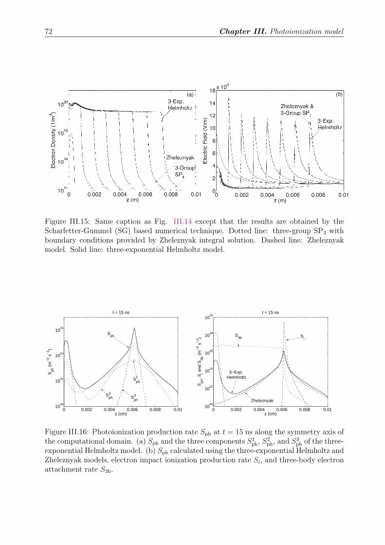
72 Chapter III. Photoionization model
Figure III.15: Same caption as Fig. III.14 except that the results are obtained by theScharfetter-Gummel (SG) based numerical technique. Dotted line: three-group SP3 withboundary conditions provided by Zheleznyak integral solution. Dashed line: Zheleznyakmodel. Solid line: three-exponential Helmholtz model.
0 0.002 0.004 0.006 0.008 0.0110
20
1022
1024
1026
z (cm)
Sph
(m
−3 s
−1 )
t = 15 ns
Sph
Sph1
Sph2
Sph3
0 0.002 0.004 0.006 0.008 0.0110
20
1022
1024
1026
1028
1030
z (cm)
Sph
, Si a
nd S
3b (
m−
3 s−
1 )
t = 15 ns
Si
3−Exp. Helmholtz
Zheleznyak
S3b
Figure III.16: Photoionization production rate Sph at t = 15 ns along the symmetry axis ofthe computational domain. (a) Sph and the three components S1
ph, S2ph, and S3
ph of the three-exponential Helmholtz model. (b) Sph calculated using the three-exponential Helmholtz andZheleznyak models, electron impact ionization production rate Si, and three-body electronattachment rate S3b.
III.7. Conclusions 73
Figure III.16(b) compares the photoionization source term calculated by the three-exponentialHelmholtz model and the optimized integral Zheleznyak model, the electron impact ioniza-tion rate, and the three-body electron attachment rate. For the photoionization productionrate, results from both models are in a very good agreement in the region of, and aheadof the streamer head. A significant difference is observed in the region near the sphericalelectrode. As already discussed for the double-headed streamer test-case, the optimizedintegral solution does not include contributions from the emission sources outside of theregion around the streamer head, but the Helmholtz solution does. A relatively strongphotoionization appears in the region near the spherical electrode implying strong pho-ton emission source in this region. The Helmholtz model automatically accounts for thissource when solving the Helmholtz differential equation. The agreement of the modelingresults obtained using the two photoionization models shown by Fig. III.15 suggests thatthe different photoionization rates in the region near spherical electrode do not affect thedynamics of the streamer, which is mostly controlled by photons emitted by the streamerhead.
Figure III.16(b) further indicates that in contrast to the high applied field case, for whichelectron impact ionization was a dominant process controlling production and loss of elec-trons in the entire simulation domain (including streamer head and streamer channel re-gions), the low field case is characterized by the dominance of three-body attachment inthe body of the streamer, the dominance of the electron impact ionization in the streamerhead, and the dominance of photoionization in the region ahead of the streamer head.
III.7 Conclusions
In this chapter, we discussed and improved several models currently proposed in the lit-erature for calculation of the photoionization produced by plasma discharges in air. Inparticular, the classical Zheleznyak integral model and three photoionization models in adifferential form are presented. The reported improvements of the differential models areachieved by more accurate accounting for the spectral dependence of the photoionizationprocess. The different approaches presented in this chapter can be directly applied forphotoionization calculations in model studies of the dynamics of streamers in air.
An efficient implementation of the classical Zheleznyak integral model is presented forstreamer modeling in air. The three differential approaches developed are a three-exponentialHelmholtz model, a three-group Eddington, and a three-group improved Eddington (SP3)models. The Helmholtz model is based on an approximation of the absorption functionof the gas in order to transform the integral expression of the photoionization term in aset of Helmholtz differential equations. The Eddington and SP3 methods are based onthe direct numerical solution of an approximation of the radiative transfer equation. It isdemonstrated that the solutions involved in all three differential models require accuratedefinition of the boundary conditions.
We have conducted three test studies of the performance of the newly proposed pho-toionization models: Gaussian emission source, a double-headed streamer developing ina strong uniform electric field (greater than the conventional breakdown field) and the pos-itive streamer propagation in weak external fields (less than the conventional breakdownfield).
74 Chapter III. Photoionization model
Our studies using the Gaussian source have demonstrated that the use of a three-exponentialfit to the absorption function in air either with the Eddington, SP3 or the Helmholtz modelallows to obtain a good agreement with the Zheleznyak integral model, and that single ortwo-exponential fits do not allow to reproduce the Zheleznyak model accurately. We havealso demonstrated that a proper setting of boundary conditions improves significantly theagreement between the Zheleznyak model and the three differential models.
Our model studies of the double-headed streamer have demonstrated that with the three-group Eddington, the three-group SP3, or the three-exponential Helmholtz models, thecalculated streamers are very similar to the one calculated using the classical Zheleznyakintegral model. It is particularly interesting to note that Eddington and SP3 models, whichare in principle only very well suited to situations in which photon absorption is sufficientlyhigh, can be used to calculate very accurately the photoionization source term using athree-group approach even if some effective absorption coefficients in the model are small.The comparison of the photoionization and ionization source terms for the studied case ofstrong uniform applied field indicates that photoionization only plays a role during the veryearly stage of the development of the streamer.
Our studies on the propagation of a positive streamer in a weak field have demonstratedthat with the three-group SP3, or the three-exponential Helmholtz models, the calculatedstreamers are very similar to the one calculated using the classical Zheleznyak integralmodel. It is important to note that in this case, the streamer dynamics is much moreaffected by the photoionization than in the external high-field propagation case.
In this work, we have also compared streamer modeling results obtained using differentnumerical techniques to solve the transport equations for charged particles: the Zalesak flux-corrected transport (FCT) method and the modified Scharfetter–Gummel (SG) algorithm.We have also utilized different techniques for solution of the Poisson’s field equation: theD03EBF module of the NAG Fortran library and the SOR method, which are used inconjunction with the FCT and SG transport algorithms, respectively. Moreover, we haverealized tests with the direct solver SuperLU which completely confirm the obtained resultswith the iterative solvers. The results of solution of the same streamer problem obtainedby the FCT method based on a 3rd order QUICKEST scheme and an upwind scheme, andby the modified SG algorithm demonstrate that both numerical techniques lead to accurateand consistent solutions of the streamer problem.
The results of accurate measurement of computational time involved in calculations usingdifferent photoionization models for the considered modeled streamer are presented, whichindicate, in particular, that the computational times of the differential and optimized in-tegral models for the model case considered in the present study are of the same order.However, it is important to mention that a significant acceleration of the integral modelsin simple cases of single or double-headed streamers studied with these models to date hasbeen possible due to introduction of moving meshes with variable cell sizes and employ-ment of effective windowing and interpolation techniques. The details of related algorithmsare presented in the present chapter. It is important to stress that the optimization ofthe integral model is rather complex and requires to be separately adapted to every newconfiguration studied. Conversely, the implementation of the photoionization models basedon differential equation approach is straightforward and simple. Furthermore, in the opti-mized integral approach the photoionization source term is calculated accurately only closeto the streamer heads. For example, in the double-headed test-case, we have shown that in
III.7. Conclusions 75
the optimized integral model the photoionization source term is not calculated accuratelyin the region between the streamer heads (see discussion of Figure III.11(b) in SectionIII.6.2). Conversely with the differential approaches the photoionization term is calculatedaccurately in the whole computation domain.
Although the different photoionization models are only used to model streamer dischargesin air in this study, we expect that the models can be applied to evaluating the photoion-ization effects in other forms of plasma discharges in air. In addition, the extension ofthe photoionization models to other gases is possible if the information on all emission,absorption and photoionization coefficients of the studied gas is available.
The presented results document the range of applicability of the newly developed pho-toionization models and emphasize that the accurate formulation of boundary conditionsrepresents an important task needed for a successful extension of the proposed formula-tions to two- and three-dimensional physical systems with obstacles of complex geometry(i.e., electrodes, dust particles, aerosols, etc.), which are opaque for the photoionizing UVphotons. We have demonstrated that accurate definition of the boundary conditions canbe effectively introduced with the Zheleznyak integral model. For the Eddington modelwe have also demonstrated performance of a set of boundary conditions consistent withthe first order approximation of the radiative transfer equation, the so-called Marshak’sboundary conditions (III.30). These boundary conditions are simple, fast to compute andeasy to adapt to any configuration. This is also possible with the SP3 model by using theLarsen’s boundary conditions (III.31). The possibility to formulate such a consistent setof equations and boundary conditions based on radiative transfer physics is a significantadvantage of the Eddington and SP3 models in comparison with the Helmholtz model.
We emphasize that the actual advantage of differential models advanced in this chapter incomparison with the integral model lies in the simplicity of implementation of this type ofmodels, and in unquestionable simplicity of extension of these models to complex two- andthree-dimensional simulation geometries, involving, for example, propagation of multiplestreamer heads in the same simulation domain, and the presence of obstacles on the streamerpath (i.e., electrodes, dust particles, aerosols, etc).
Finally, it is important to note that in this work we have used only approximate solutions ofthe radiative transfer equation. Capeillère et al. [2008] have used a Finite Volume Method(FVM) on space and angular variables has been used to solve directly the radiative transferequation. It is important to note that the FVM method is much more complex to implementthan approximate differential models presented in this chapter. The FVM method wasvalidated by comparison with the reference integral solution on a monochromatic Gaussiansource. When the absorption coefficient is high enough, Eddington and SP3 methods areas accurate and become faster than the direct method. However, when the absorptioncoefficient decreases, approximate methods become less accurate and more computationallyexpensive than the direct FVM. Therefore the direct method was applied in [Capeillèreet al., 2008] to the simulation of a double-headed streamer at ground pressure assuming thatphotoionization is monochromatic. The results obtained have been compared with thoseobtained with the SP3 model and further validate the use of the SP3 model for sufficientlyhigh values of the absorption coefficient. In [Capeillère et al., 2008], only monochromaticcases have been studied. To accurately simulate streamers propagating in air at atmosphericpressure, it is necessary to take into account the spectral dependence of the photoionizationprocess. The three-group approach presented in this chapter could be very easily used with

76 Chapter III. Photoionization model
the FVM to simulate streamer propagation in air in high and weak fields. The relatedresults will be presented in a separate dedicated work.
Chapter IV
The use of a Ghost Fluid Method forPoisson’s equation in complexgeometries
Table of ContentsIV.1 Introduction . . . . . . . . . . . . . . . . . . . . . . . . . . . . . . 78
IV.2 Model formulation . . . . . . . . . . . . . . . . . . . . . . . . . . . 80
IV.2.1 The Ghost Fluid Method applied to Poisson’s equation . . . . . 80
IV.2.2 Analytical solution of Laplace’s equation in hyperbolic point-to-point and point-to-plane geometries . . . . . . . . . . . . . . . . 84
IV.2.3 Numerical methods for Poisson’s equation and drift-diffusion equa-tions . . . . . . . . . . . . . . . . . . . . . . . . . . . . . . . . . . 85
IV.3 Results and Discussion . . . . . . . . . . . . . . . . . . . . . . . . 86
IV.3.1 Laplacian field in a point-to-plane geometry . . . . . . . . . . . . 86
IV.3.2 Positive streamer propagation in a point-to-plane geometry . . . 89
IV.3.3 Streamer propagation in point-to-point geometry . . . . . . . . . 92
Discharge at 1000 K . . . . . . . . . . . . . . . . . . . . . . . . . 93
Discharge at 300 K . . . . . . . . . . . . . . . . . . . . . . . . . . 98
Discharge at 1800 K . . . . . . . . . . . . . . . . . . . . . . . . . 98
IV.4 Conclusions . . . . . . . . . . . . . . . . . . . . . . . . . . . . . . . 102
78 Chapter IV. The use of a Ghost Fluid Method
IV.1 Introduction
Many early simulation studies on streamers have been done in the simple plane-to-plane geometry [Dhali and Williams , 1987; Vitello et al., 1994; Kulikovsky , 1997b].
However, in practical situations, the electrode geometries are much more complex, oftenwith one of the electrodes having a much smaller radius of curvature than the other (e.g.,point-to-plane, wire-to-cylinder). One of the most studied configurations in the literatureis the point-to-plane geometry. In Chapters II and III we studied a “sphere-to-plane”configuration, proposed by Babaeva and Naidis [1996], taking into account the influence ofthe spherical electrode on the discharge without including it in the computational domain.In this model, the computational grid is tangent to the sphere, and therefore there is onlyone point of contact between the spherical electrode and the computational domain. Thesimulation of the discharge is roughly approximated close to the sphere, in regions wherethe computational grid has no contact with the electrode. It is interesting to note that thisapproach is rather easy to implement and has been used in different works in the recent fewyears [Liu and Pasko, 2006; Liu et al., 2007]. The only complexity of this model is in theimplementation of the boundary conditions for Poisson’s equation, where image charges inthe sphere have to be taken into account (see Section II.1.2).
For more realistic electrode shapes, such as for hyperboloids [Kulikovsky , 1997b; Morrowand Lowke, 1997; Pancheshnyi et al., 2001] or paraboloids [Djermoune et al., 1995a, b;Dessantes , 2000], the electrode is usually included in the computational domain. However,as most streamer simulations are carried out using a finite volume approach and a rectilineargrid, the shape of the electrode is approximated by a staircase.
In the works of Morrow and Lowke [1997], Djermoune et al. [1995a, b], and Dessantes[2000], the shape of the electrode is defined as accurately as possible by defining a newaxial grid point for each radial grid point, such that the position defined by the axialand radial coordinates lies on the electrode surface. This definition of the grid allows fordefining the potential on the electrode surface very accurately, which serves as the bound-ary condition for Poisson’s equation. However, the use of this approach for hyperboloidsand paraboloids leads to significant variations of the cell sizes to adapt to the point elec-trode shape. In finite volume methods, these significant variations of cell sizes are notrecommended. Furthermore, with this approach, the grid has to be adapted to each newgeometry.
Another approach is to use a curvilinear grid [Kim et al., 2004; Akishev et al., 2002]. Forexample, for a hyperboloid-to-plane geometry, a quasi-orthogonal grid can be defined basedon confocal hyperboloids and ellipses. In this case, the grid is orthogonal to the electrodesurface, therefore the potential of the electrode is set very accurately. Furthermore, with
IV.1. Introduction 79
this approach, it is rather easy to implement boundary conditions for charged species withvarious secondary emission processes. However, in this case also, the grid has to be adaptedto each new geometry.
Finally, some authors [Georghiou et al., 1999; Papageorghiou and Spyrou, 2007] use finite-element methods with unstructured grids to simulate streamer propagation in wire-to-plane or point-to-plane geometries. It is clear that the use of an unstructured grid allowsfor an accurate local description of complex geometries with a reduced number of pointsin comparison to structured grids. Recently, Ducasse et al. [2007] have compared theresults obtained with finite volume and finite element approaches with structured andunstructured grids, respectively, for a point-to-plane geometry with a 1-mm inter-electrodegap and a hyperboloid anode. Good agreement between the results obtained with bothmethods has been observed. However, it is important to note that the implementation ofthe finite element method is much more complex than the finite volume approach. Ducasseet al. [2007] have also shown that even with a smaller number of nodes in the grid, thecomputational cost of finite element method calculations appeared to be much higher thanthat of finite volume method calculations.
In the work reported in this chapter, we have implemented a method allowing to easilytake into account electrodes of complex geometries in streamer simulations. For simplicity,we have tried to find a method based on rectilinear grids and finite volume or differenceapproaches. The problem of taking into account a boundary or an interface of complexgeometry in a rectilinear grid has been studied in fluid mechanics. For example, to modelinterfaces in two-phase flows, Fedkiw et al. [1999] have introduced the Ghost Fluid Method(GFM). This method accurately localizes the interface, follows its time evolution witha Level Set formalism [Liu et al., 2000], and gives the possibility of accurately definingboundary conditions at the interface. Liu et al. [2000] developed the method for the variablecoefficient Poisson’s equation. Kang et al. [2000] subsequently extended it to treat two-phaseincompressible flow, including the effects of viscosity, surface tension, and gravity. Nguyenet al. [2001] included the reactivity of the flows. For Dirichlet boundary conditions setat the interface, the second-order-accurate symmetric discretization of Poisson’s equationbased on the GFM was obtained in [Gibou et al., 2002]. A review of boundary conditioncapturing methods based on the GFM is provided in [Hong et al., 2007].
Preliminary tests in applying the GFM to the simulation of a streamer discharge have beendone by Régnier [2004]. In contrast to two-phase flows, the situation is simpler for streamersimulations since the embedded boundary (the electrode) is motionless. In this work, wewill apply the GFM to the simulation of streamer discharge propagation in the classicalpoint-to-plane and point-to-point geometries.
In Section IV.2, we present the equations needed for the numerical simulation of streamerdischarges and the application of the GFM to Poisson’s equation. In Section IV.3, tovalidate the use of the GFM for the computation of the Laplacian electric potential and ofthe electric field, we compare the results obtained using this approach with the analyticalsolution in a point-to-plane configuration. Then, in order to validate the use of the GhostFluid Method for streamer simulations, we compare the results obtained using the GFMwith the results obtained by Kulikovsky [1998] for the same point-to-plane configuration.Finally, the application of the GFM to the simulation of a discharge in preheated air in apoint-to-point geometry is presented and discussed.
80 Chapter IV. The use of a Ghost Fluid Method
IV.2 Model formulation
As stated in Section I.4, the starting point of our streamer simulations is the resolution ofEquations (I.28)–(I.30) coupled to Poisson’s equation (I.31).
It is important to note that for streamer simulations, the electric field is a key parameter.First, transport parameters and source terms in Equations (I.28)–(I.30) have a strong non-linear dependence on it. Second, the electric field is directly related to charged speciesdensities in Equation (I.31). Therefore the simulation of streamer propagation requiresan accurate calculation of the electric field in the simulation domain at each time step,especially in regions with high gradients in the field (e.g., the streamer head and the tip ofthe needle electrode). In the following section, we present the application of the GFM toPoisson’s equation to calculate accurately the potential and the electric field in streamersimulations.
IV.2.1 The Ghost Fluid Method applied to Poisson’s equation
We use the scheme presented in Section II.1.1 for the numerical resolution of Poisson’sequation. In the volume of the computational domain (i.e., far from the boundaries) thesecond order finite difference discretization of Equation (II.1) in cylindrical coordinatesgives the classical five diagonal linear system:
V ei,jVi+1,j + V w
i,jVi−1,j + V si,jVi,j−1 + V n
i,jVi,j+1 + V ci,jVi,j = −ρi,j
ǫ0
(IV.1)
where the usual coefficients V ei,j, V w
i,j, V ni,j, V s
i,j, V ci,j of the grid node (i, j) with coordinates
(xi, rj) in the simulation domain (i.e., far from the boundaries) are given by Equation (II.3).
As shown in Figure IV.1, the electrode is an embedded boundary in the Cartesian grid.To localize the fluid/electrode interface accurately, we use two “signed distance functions”based on the Level Set formalism (see [Liu et al., 2000]): φx
i,j is defined by the distancebetween grid nodes and the electrode interface according to x, and φr
i,j is defined by thedistance between grid nodes and the electrode interface according to r. In Figure IV.1, wedefine θj and βi such that |φx
i,j| = θj∆xi−1 and |φri,j| = βi∆rj−1. The distance functions
are readily found if one has an analytical expression of the electrode interface. Distancefunctions are defined as negative for nodes inside the electrode and as positive for nodesin the computational domain. For example, in Figure IV.1, the node (i, j) is outsidethe electrode, and therefore the distance functions (or Level Set functions) are definedas positive for this node.
Through the fluid/electrode interface, the potential is continuous, but there is a jump in theelectric field. The GFM consists in setting virtual potentials (denoted by the superscript“G” for “ghost” in the following) at the nodes inside the electrode (e.g., V G
i−1 at the i − 1node in Figure IV.2) such that the interpolated potential at the interface between two nodesof the grid is precisely the physical potential of the electrode VI (see Figure IV.2). For theinterpolation, in this work we have used a linear interpolation both in x and r. This is arefinement of the Dirichlet boundary condition over the electrode surface which was usedin Gibou et al. [2002].
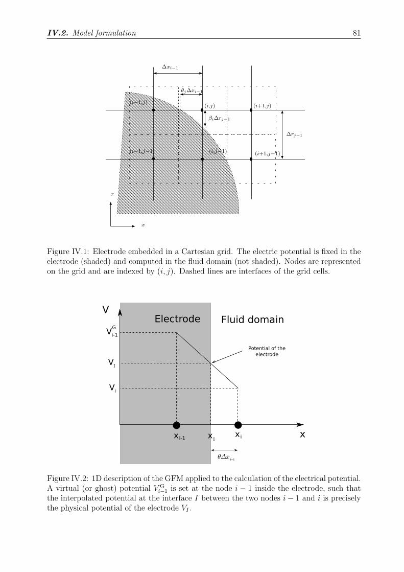
IV.2. Model formulation 81
θj∆xi−1
βi∆rj−1
∆xi−1
∆rj−1
(i−1,j)(i,j) (i+1,j)
(i−1,j−1) (i,j−1) (i+1,j−1)
r
x
Figure IV.1: Electrode embedded in a Cartesian grid. The electric potential is fixed in theelectrode (shaded) and computed in the fluid domain (not shaded). Nodes are representedon the grid and are indexed by (i, j). Dashed lines are interfaces of the grid cells.
Figure IV.2: 1D description of the GFM applied to the calculation of the electrical potential.A virtual (or ghost) potential V G
i−1 is set at the node i − 1 inside the electrode, such thatthe interpolated potential at the interface I between the two nodes i − 1 and i is preciselythe physical potential of the electrode VI .
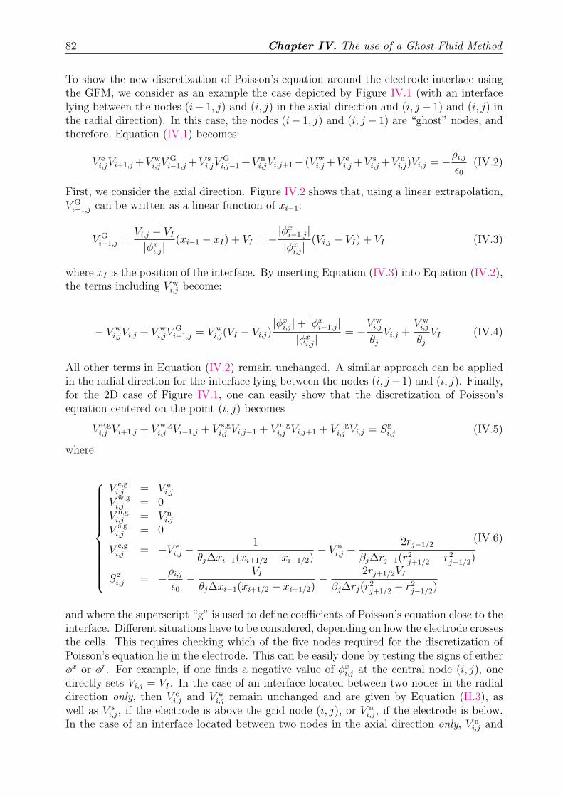
82 Chapter IV. The use of a Ghost Fluid Method
To show the new discretization of Poisson’s equation around the electrode interface usingthe GFM, we consider as an example the case depicted by Figure IV.1 (with an interfacelying between the nodes (i− 1, j) and (i, j) in the axial direction and (i, j − 1) and (i, j) inthe radial direction). In this case, the nodes (i− 1, j) and (i, j − 1) are “ghost” nodes, andtherefore, Equation (IV.1) becomes:
V ei,jVi+1,j +V w
i,jVGi−1,j +V s
i,jVGi,j−1 +V n
i,jVi,j+1− (V wi,j +V e
i,j +V si,j +V n
i,j)Vi,j = −ρi,j
ǫ0
(IV.2)
First, we consider the axial direction. Figure IV.2 shows that, using a linear extrapolation,V G
i−1,j can be written as a linear function of xi−1:
V Gi−1,j =
Vi,j − VI
|φxi,j|
(xi−1 − xI) + VI = −|φx
i−1,j||φx
i,j|(Vi,j − VI) + VI (IV.3)
where xI is the position of the interface. By inserting Equation (IV.3) into Equation (IV.2),the terms including V w
i,j become:
− V wi,jVi,j + V w
i,jVGi−1,j = V w
i,j(VI − Vi,j)|φx
i,j| + |φxi−1,j|
|φxi,j|
= −V w
i,j
θj
Vi,j +V w
i,j
θj
VI (IV.4)
All other terms in Equation (IV.2) remain unchanged. A similar approach can be appliedin the radial direction for the interface lying between the nodes (i, j−1) and (i, j). Finally,for the 2D case of Figure IV.1, one can easily show that the discretization of Poisson’sequation centered on the point (i, j) becomes
V e,gi,j Vi+1,j + V w,g
i,j Vi−1,j + V s,gi,j Vi,j−1 + V n,g
i,j Vi,j+1 + V c,gi,j Vi,j = Sg
i,j (IV.5)
where
V e,gi,j = V e
i,j
V w,gi,j = 0
V n,gi,j = V n
i,j
V s,gi,j = 0
V c,gi,j = −V e
i,j −1
θj∆xi−1(xi+1/2 − xi−1/2)− V n
i,j −2rj−1/2
βj∆rj−1(r2j+1/2 − r2
j−1/2)
Sgi,j = −ρi,j
ǫ0
− VI
θj∆xi−1(xi+1/2 − xi−1/2)− 2rj+1/2VI
βj∆rj(r2j+1/2 − r2
j−1/2)
(IV.6)
and where the superscript “g” is used to define coefficients of Poisson’s equation close to theinterface. Different situations have to be considered, depending on how the electrode crossesthe cells. This requires checking which of the five nodes required for the discretization ofPoisson’s equation lie in the electrode. This can be easily done by testing the signs of eitherφx or φr. For example, if one finds a negative value of φx
i,j at the central node (i, j), onedirectly sets Vi,j = VI . In the case of an interface located between two nodes in the radialdirection only, then V e
i,j and V wi,j remain unchanged and are given by Equation (II.3), as
well as V si,j, if the electrode is above the grid node (i, j), or V n
i,j, if the electrode is below.In the case of an interface located between two nodes in the axial direction only, V n
i,j and
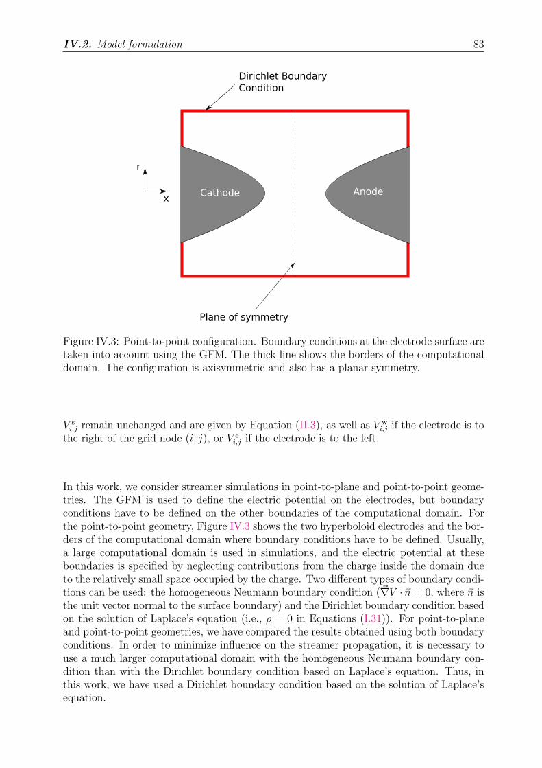
IV.2. Model formulation 83
Figure IV.3: Point-to-point configuration. Boundary conditions at the electrode surface aretaken into account using the GFM. The thick line shows the borders of the computationaldomain. The configuration is axisymmetric and also has a planar symmetry.
V si,j remain unchanged and are given by Equation (II.3), as well as V w
i,j if the electrode is tothe right of the grid node (i, j), or V e
i,j if the electrode is to the left.
In this work, we consider streamer simulations in point-to-plane and point-to-point geome-tries. The GFM is used to define the electric potential on the electrodes, but boundaryconditions have to be defined on the other boundaries of the computational domain. Forthe point-to-point geometry, Figure IV.3 shows the two hyperboloid electrodes and the bor-ders of the computational domain where boundary conditions have to be defined. Usually,a large computational domain is used in simulations, and the electric potential at theseboundaries is specified by neglecting contributions from the charge inside the domain dueto the relatively small space occupied by the charge. Two different types of boundary condi-tions can be used: the homogeneous Neumann boundary condition (~∇V ·~n = 0, where ~n isthe unit vector normal to the surface boundary) and the Dirichlet boundary condition basedon the solution of Laplace’s equation (i.e., ρ = 0 in Equations (I.31)). For point-to-planeand point-to-point geometries, we have compared the results obtained using both boundaryconditions. In order to minimize influence on the streamer propagation, it is necessary touse a much larger computational domain with the homogeneous Neumann boundary con-dition than with the Dirichlet boundary condition based on Laplace’s equation. Thus, inthis work, we have used a Dirichlet boundary condition based on the solution of Laplace’sequation.
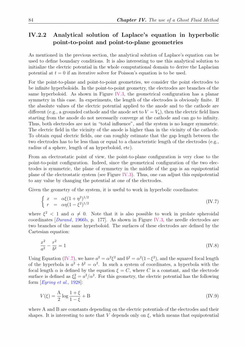
84 Chapter IV. The use of a Ghost Fluid Method
IV.2.2 Analytical solution of Laplace’s equation in hyperbolicpoint-to-point and point-to-plane geometries
As mentioned in the previous section, the analytical solution of Laplace’s equation can beused to define boundary conditions. It is also interesting to use this analytical solution toinitialize the electric potential in the whole computational domain to derive the Laplacianpotential at t = 0 if an iterative solver for Poisson’s equation is to be used.
For the point-to-plane and point-to-point geometries, we consider the point electrodes tobe infinite hyperboloids. In the point-to-point geometry, the electrodes are branches of thesame hyperboloid. As shown in Figure IV.3, the geometrical configuration has a planarsymmetry in this case. In experiments, the length of the electrodes is obviously finite. Ifthe absolute values of the electric potential applied to the anode and to the cathode aredifferent (e.g., a grounded cathode and the anode set to V = Va), then the electric field linesstarting from the anode do not necessarily converge at the cathode and can go to infinity.Thus, both electrodes are not in “total influence”, and the system is no longer symmetric.The electric field in the vicinity of the anode is higher than in the vicinity of the cathode.To obtain equal electric fields, one can roughly estimate that the gap length between thetwo electrodes has to be less than or equal to a characteristic length of the electrodes (e.g.,radius of a sphere, length of an hyperboloid, etc).
From an electrostatic point of view, the point-to-plane configuration is very close to thepoint-to-point configuration. Indeed, since the geometrical configuration of the two elec-trodes is symmetric, the plane of symmetry in the middle of the gap is an equipotentialplane of the electrostatic system (see Figure IV.3). Thus, one can adjust this equipotentialto any value by changing the potential at one of the electrodes.
Given the geometry of the system, it is useful to work in hyperbolic coordinates:
x = αξ(1 + η2)1/2
r = αη(1 − ξ2)1/2 (IV.7)
where ξ2 < 1 and α 6= 0. Note that it is also possible to work in prolate spheroidalcoordinates [Durand , 1966b, p. 177]. As shown in Figure IV.3, the needle electrodes aretwo branches of the same hyperboloid. The surfaces of these electrodes are defined by theCartesian equation:
x2
a2− r2
b2= 1 (IV.8)
Using Equation (IV.7), we have a2 = α2ξ2 and b2 = α2(1−ξ2), and the squared focal lengthof the hyperbola is a2 + b2 = α2. In such a system of coordinates, a hyperbola with thefocal length α is defined by the equation ξ = C, where C is a constant, and the electrodesurface is defined as ξ2
0 = a2/α2. For this geometry, the electric potential has the followingform [Eyring et al., 1928]:
V (ξ) =A
2log
1 + ξ
1 − ξ+ B (IV.9)
where A and B are constants depending on the electric potentials of the electrodes and theirshapes. It is interesting to note that V depends only on ξ, which means that equipotential
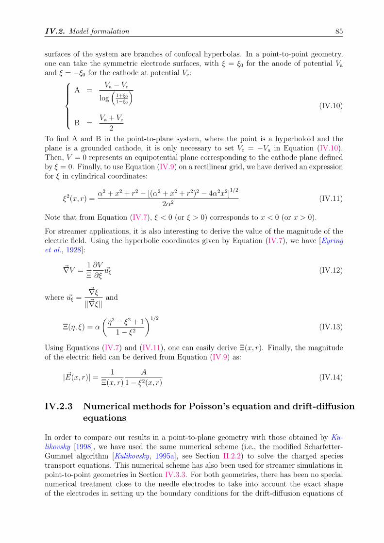
IV.2. Model formulation 85
surfaces of the system are branches of confocal hyperbolas. In a point-to-point geometry,one can take the symmetric electrode surfaces, with ξ = ξ0 for the anode of potential Va
and ξ = −ξ0 for the cathode at potential Vc:
A =Va − Vc
log(
1+ξ01−ξ0
)
B =Va + Vc
2
(IV.10)
To find A and B in the point-to-plane system, where the point is a hyperboloid and theplane is a grounded cathode, it is only necessary to set Vc = −Va in Equation (IV.10).Then, V = 0 represents an equipotential plane corresponding to the cathode plane definedby ξ = 0. Finally, to use Equation (IV.9) on a rectilinear grid, we have derived an expressionfor ξ in cylindrical coordinates:
ξ2(x, r) =α2 + x2 + r2 − [(α2 + x2 + r2)2 − 4α2x2]
1/2
2α2(IV.11)
Note that from Equation (IV.7), ξ < 0 (or ξ > 0) corresponds to x < 0 (or x > 0).
For streamer applications, it is also interesting to derive the value of the magnitude of theelectric field. Using the hyperbolic coordinates given by Equation (IV.7), we have [Eyringet al., 1928]:
~∇V =1
Ξ
∂V
∂ξ~uξ (IV.12)
where ~uξ =~∇ξ
‖~∇ξ‖and
Ξ(η, ξ) = α
(
η2 − ξ2 + 1
1 − ξ2
)1/2
(IV.13)
Using Equations (IV.7) and (IV.11), one can easily derive Ξ(x, r). Finally, the magnitudeof the electric field can be derived from Equation (IV.9) as:
| ~E(x, r)| =1
Ξ(x, r)
A
1 − ξ2(x, r)(IV.14)
IV.2.3 Numerical methods for Poisson’s equation and drift-diffusionequations
In order to compare our results in a point-to-plane geometry with those obtained by Ku-likovsky [1998], we have used the same numerical scheme (i.e., the modified Scharfetter-Gummel algorithm [Kulikovsky , 1995a], see Section II.2.2) to solve the charged speciestransport equations. This numerical scheme has also been used for streamer simulations inpoint-to-point geometries in Section IV.3.3. For both geometries, there has been no specialnumerical treatment close to the needle electrodes to take into account the exact shapeof the electrodes in setting up the boundary conditions for the drift-diffusion equations of
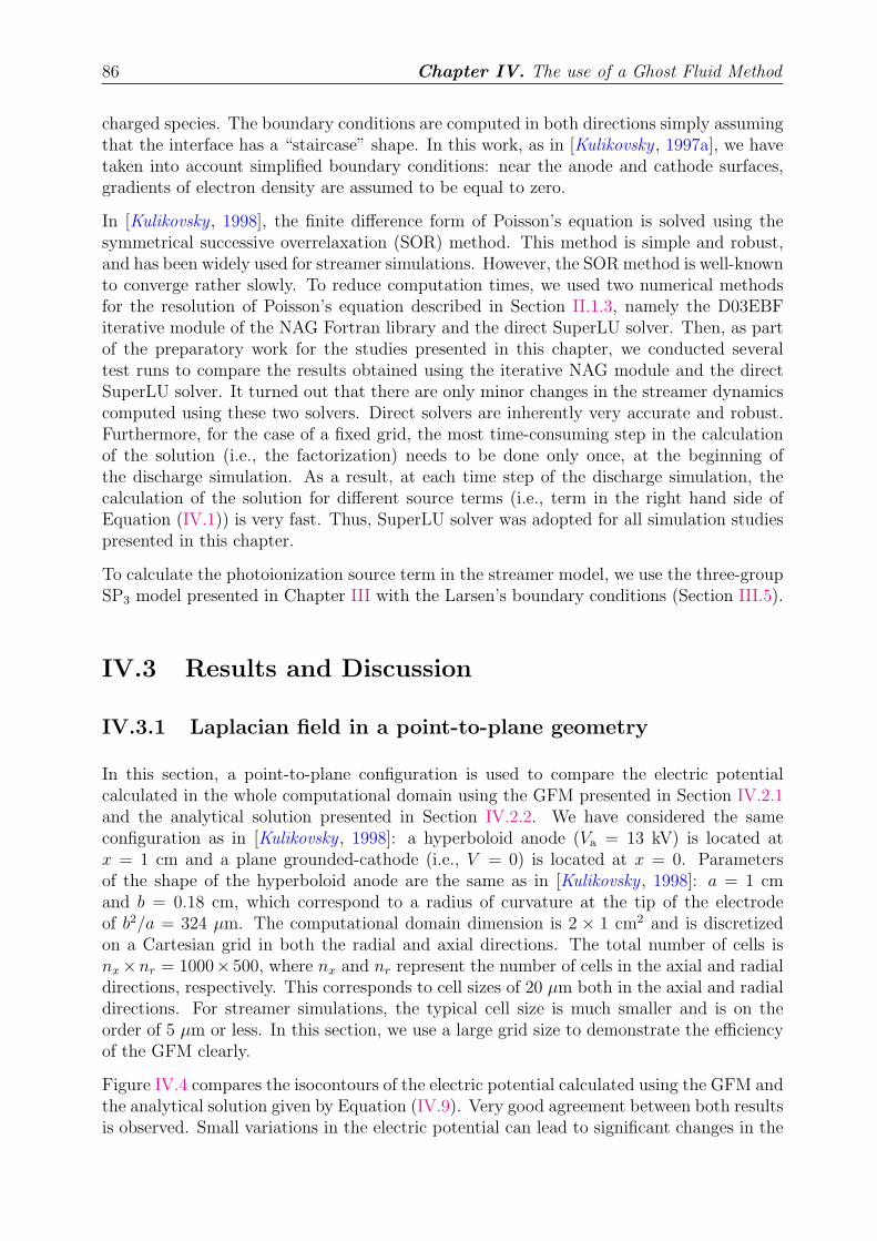
86 Chapter IV. The use of a Ghost Fluid Method
charged species. The boundary conditions are computed in both directions simply assumingthat the interface has a “staircase” shape. In this work, as in [Kulikovsky , 1997a], we havetaken into account simplified boundary conditions: near the anode and cathode surfaces,gradients of electron density are assumed to be equal to zero.
In [Kulikovsky , 1998], the finite difference form of Poisson’s equation is solved using thesymmetrical successive overrelaxation (SOR) method. This method is simple and robust,and has been widely used for streamer simulations. However, the SOR method is well-knownto converge rather slowly. To reduce computation times, we used two numerical methodsfor the resolution of Poisson’s equation described in Section II.1.3, namely the D03EBFiterative module of the NAG Fortran library and the direct SuperLU solver. Then, as partof the preparatory work for the studies presented in this chapter, we conducted severaltest runs to compare the results obtained using the iterative NAG module and the directSuperLU solver. It turned out that there are only minor changes in the streamer dynamicscomputed using these two solvers. Direct solvers are inherently very accurate and robust.Furthermore, for the case of a fixed grid, the most time-consuming step in the calculationof the solution (i.e., the factorization) needs to be done only once, at the beginning ofthe discharge simulation. As a result, at each time step of the discharge simulation, thecalculation of the solution for different source terms (i.e., term in the right hand side ofEquation (IV.1)) is very fast. Thus, SuperLU solver was adopted for all simulation studiespresented in this chapter.
To calculate the photoionization source term in the streamer model, we use the three-groupSP3 model presented in Chapter III with the Larsen’s boundary conditions (Section III.5).
IV.3 Results and Discussion
IV.3.1 Laplacian field in a point-to-plane geometry
In this section, a point-to-plane configuration is used to compare the electric potentialcalculated in the whole computational domain using the GFM presented in Section IV.2.1and the analytical solution presented in Section IV.2.2. We have considered the sameconfiguration as in [Kulikovsky , 1998]: a hyperboloid anode (Va = 13 kV) is located atx = 1 cm and a plane grounded-cathode (i.e., V = 0) is located at x = 0. Parametersof the shape of the hyperboloid anode are the same as in [Kulikovsky , 1998]: a = 1 cmand b = 0.18 cm, which correspond to a radius of curvature at the tip of the electrodeof b2/a = 324 µm. The computational domain dimension is 2 × 1 cm2 and is discretizedon a Cartesian grid in both the radial and axial directions. The total number of cells isnx ×nr = 1000× 500, where nx and nr represent the number of cells in the axial and radialdirections, respectively. This corresponds to cell sizes of 20 µm both in the axial and radialdirections. For streamer simulations, the typical cell size is much smaller and is on theorder of 5 µm or less. In this section, we use a large grid size to demonstrate the efficiencyof the GFM clearly.
Figure IV.4 compares the isocontours of the electric potential calculated using the GFM andthe analytical solution given by Equation (IV.9). Very good agreement between both resultsis observed. Small variations in the electric potential can lead to significant changes in the
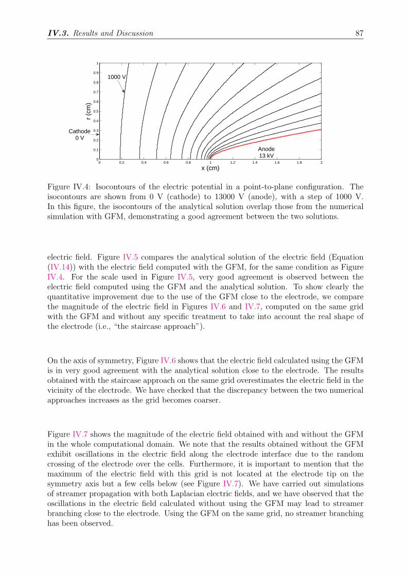
IV.3. Results and Discussion 87
x (cm)
r (c
m)
0 0.2 0.4 0.6 0.8 1 1.2 1.4 1.6 1.8 20
0.1
0.2
0.3
0.4
0.5
0.6
0.7
0.8
0.9
1
1000 V
Cathode0 V
Anode13 kV
Figure IV.4: Isocontours of the electric potential in a point-to-plane configuration. Theisocontours are shown from 0 V (cathode) to 13000 V (anode), with a step of 1000 V.In this figure, the isocontours of the analytical solution overlap those from the numericalsimulation with GFM, demonstrating a good agreement between the two solutions.
electric field. Figure IV.5 compares the analytical solution of the electric field (Equation(IV.14)) with the electric field computed with the GFM, for the same condition as FigureIV.4. For the scale used in Figure IV.5, very good agreement is observed between theelectric field computed using the GFM and the analytical solution. To show clearly thequantitative improvement due to the use of the GFM close to the electrode, we comparethe magnitude of the electric field in Figures IV.6 and IV.7, computed on the same gridwith the GFM and without any specific treatment to take into account the real shape ofthe electrode (i.e., “the staircase approach”).
On the axis of symmetry, Figure IV.6 shows that the electric field calculated using the GFMis in very good agreement with the analytical solution close to the electrode. The resultsobtained with the staircase approach on the same grid overestimates the electric field in thevicinity of the electrode. We have checked that the discrepancy between the two numericalapproaches increases as the grid becomes coarser.
Figure IV.7 shows the magnitude of the electric field obtained with and without the GFMin the whole computational domain. We note that the results obtained without the GFMexhibit oscillations in the electric field along the electrode interface due to the randomcrossing of the electrode over the cells. Furthermore, it is important to mention that themaximum of the electric field with this grid is not located at the electrode tip on thesymmetry axis but a few cells below (see Figure IV.7). We have carried out simulationsof streamer propagation with both Laplacian electric fields, and we have observed that theoscillations in the electric field calculated without using the GFM may lead to streamerbranching close to the electrode. Using the GFM on the same grid, no streamer branchinghas been observed.
88 Chapter IV. The use of a Ghost Fluid Method
x (cm)
r (c
m)
0 0.2 0.4 0.6 0.8 1 1.2 1.4 1.6 1.8 20
0.1
0.2
0.3
0.4
0.5
0.6
0.7
0.8
0.9
1
Cathode0 V
5 kV/cm
Anode13 kV
Figure IV.5: Isocontours of the magnitude of the electric field for the same conditions asin Figure IV.4. The isocontours are shown from 1 kV/cm to 160 kV/cm, with a step of 1kV/cm. In this figure, the isocontours of the analytical solution overlap those of the electricfield computed using the GFM, demonstrating a good agreement between the two solutions.
0.98 0.985 0.99 0.995 1−1.8
−1.7
−1.6
−1.5
−1.4
−1.3
−1.2
−1.1
−1
−0.9
−0.8
−0.7x 10
5
x (cm)
Ele
ctric
fiel
d (V
/cm
)
Result with GFM
Result without GFM
Analytical solution
Figure IV.6: Magnitude of the electric field along the symmetry axis in the vicinity ofthe anode tip. Solid line: analytical solution (Equation (IV.14)). Dotted line with circles:numerical results using the GFM. Dot-dashed line with crosses: numerical results withoutthe GFM (i.e., “staircase” approach). The symbols for the numerical results correspond tothe grid nodes.
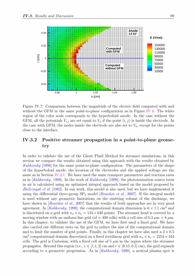
IV.3. Results and Discussion 89
x (cm)
r(c
m)
0.98 1 1.02 1.04 1.06
-0.04
-0.02
0
0.02
0.04
1500001300001100009000070000500003000010000
Anode13 kV
Computedwith GFM
Computedwithout GFM
E (V/cm)
Figure IV.7: Comparison between the magnitude of the electric field computed with andwithout the GFM in the same point-to-plane configuration as in Figure IV.4. The whiteregion of the color scale corresponds to the hyperboloid anode. In the case without theGFM, all the potentials Vi,j are set equal to Va if the point (i, j) is inside the electrode. Inthe case with GFM, the nodes inside the electrode are also set to Va, except for the pointsclose to the interface.
IV.3.2 Positive streamer propagation in a point-to-plane geome-try
In order to validate the use of the Ghost Fluid Method for streamer simulations, in thissection we compare the results obtained using this approach with the results obtained byKulikovsky [1998] for the same point-to-plane configuration. The parameters of the shapeof the hyperboloid anode, the location of the electrodes and the applied voltage are thesame as in Section IV.3.1. We have used the same transport parameters and reaction ratesas in [Kulikovsky , 1998]. In the work of Kulikovsky [1998], the photoionization source termin air is calculated using an optimized integral approach based on the model proposed byZheleznyak et al. [1982]. In our work, this model is also used, but we have implemented itusing the differential three-group SP3 model [Bourdon et al., 2007]. If the integral modelis used without any geometric limitations on the emitting volume of the discharge, wehave shown in [Bourdon et al., 2007] that the results of both approaches are in very goodagreement. In [Kulikovsky , 1998], the computational domain dimension is 6 × 1.1 cm2 andis discretized on a grid with nx ×nr = 134× 640 points. The streamer head is covered by amoving window with an uniform fine grid (of ≃ 400 cells) with a cell size of 6.3 µm × 8 µm.In this chapter, to validate the use of the GFM, we have first used a fixed grid. We havealso carried out different tests on the grid to reduce the size of the computational domainand to limit the number of grid points. Finally, in this chapter we have also used a 2× 0.5cm2 computational domain discretized on a fixed rectilinear grid with nx ×nr = 2254×344cells. The grid is Cartesian, with a fixed cell size of 5 µm in the region where the streamerpropagates. Beyond this region (i.e., x ∈ [1.1, 2] cm and r ∈ [0.15, 0.5] cm), the grid expandsaccording to a geometric progression. As in [Kulikovsky , 1998], a neutral plasma spot is
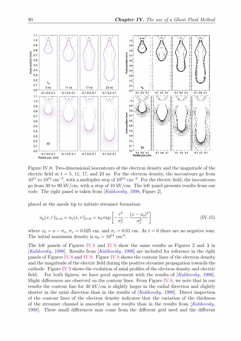
90 Chapter IV. The use of a Ghost Fluid Method
0.0
0.1
0.2
0.3
0.4
0.5
0.6
0.7
0.8
0.9
1.0
1.1
-0.1 0.0 0.1
Axia
l positio
n [
cm
]
ne
5 ns
+
-0.1 0.0 0.1
11 ns
+
-0.1 0.0 0.1
17 ns
+
-0.1 0.0 0.1
23 ns
+
0.0
0.1
0.2
0.3
0.4
0.5
0.6
0.7
0.8
0.9
1.0
1.1
-0.1 0.0 0.1
Radial pos. [cm]
|E|
+
-0.1 0.0 0.1
+
-0.1 0.0 0.1
+
-0.1 0.0 0.1
+
Figure IV.8: Two-dimensional isocontours of the electron density and the magnitude of theelectric field at t = 5, 11, 17, and 23 ns. For the electron density, the isocontours go from1011 to 1014 cm−3, with a multiplier step of 100.5 cm−3. For the electric field, the isocontoursgo from 30 to 90 kV/cm, with a step of 10 kV/cm. The left panel presents results from ourcode. The right panel is taken from [Kulikovsky , 1998, Figure 2].
placed at the anode tip to initiate streamer formation:
np(x, r)|t=0 = ne(x, r)|t=0 = n0 exp
[
− r2
σ2r
− (x − x0)2
σ2x
]
(IV.15)
where x0 = a − σx, σx = 0.025 cm, and σr = 0.01 cm. At t = 0 there are no negative ions.The initial maximum density is n0 = 1014 cm-3.
The left panels of Figures IV.8 and IV.9 show the same results as Figures 2 and 3 in[Kulikovsky , 1998]. Results from [Kulikovsky , 1998] are included for reference in the rightpanels of Figures IV.8 and IV.9. Figure IV.8 shows the contour lines of the electron densityand the magnitude of the electric field during the positive streamer propagation towards thecathode. Figure IV.9 shows the evolution of axial profiles of the electron density and electricfield. For both figures, we have good agreement with the results of [Kulikovsky , 1998].Slight differences are observed on the contour lines. From Figure IV.8, we note that in ourresults the contour line for 30 kV/cm is slightly larger in the radial direction and slightlyshorter in the axial direction than in the results of [Kulikovsky , 1998]. Direct inspectionof the contour lines of the electron density indicates that the variation of the thicknessof the streamer channel is smoother in our results than in the results from [Kulikovsky ,1998]. These small differences may come from the different grid used and the different
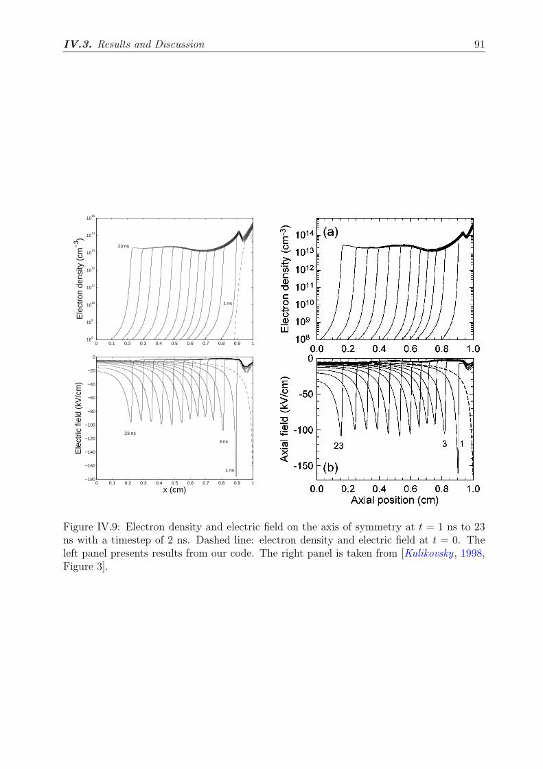
IV.3. Results and Discussion 91
0 0.1 0.2 0.3 0.4 0.5 0.6 0.7 0.8 0.9 110
8
109
1010
1011
1012
1013
1014
1015
Ele
ctro
n de
nsity
(cm
−3)
0 0.1 0.2 0.3 0.4 0.5 0.6 0.7 0.8 0.9 1−180
−160
−140
−120
−100
−80
−60
−40
−20
0
x (cm)
Ele
ctric
fiel
d (k
V/c
m)
1 ns
3 ns
23 ns
1 ns
23 ns
Figure IV.9: Electron density and electric field on the axis of symmetry at t = 1 ns to 23ns with a timestep of 2 ns. Dashed line: electron density and electric field at t = 0. Theleft panel presents results from our code. The right panel is taken from [Kulikovsky , 1998,Figure 3].
92 Chapter IV. The use of a Ghost Fluid Method
treatment of the photoinization source term in our work and from that in [Kulikovsky ,1998]. At time t = 1 ns the field in the streamer head is higher in our results than in theresults of Kulikovsky [1998]. This is possibly due to the fact that the GFM is not used in[Kulikovsky , 1998]. In Figures IV.8 and IV.9, the two phases of the streamer propagationcan be clearly observed. The first one lasts about 5 ns and corresponds to the positivestreamer formation close to the point anode and to its propagation in the high field regionclose to the electrode tip. We note that during the first phase, the streamer radius increasesas the streamer propagates towards the cathode. For t > 5 ns, the streamer propagateswith the velocity almost constant, the radius of the plasma channel and the maximumelectric field in the streamer head. In [Kulikovsky , 1998], this phase is called the stationarypropagation phase of the streamer.
The results obtained in this section clearly validate the use of the GFM for the simulationof streamer propagation.
IV.3.3 Streamer propagation in point-to-point geometry
In this section, we apply the GFM to simulate a discharge in air at atmospheric pressurebetween two point electrodes. This discharge has been studied experimentally in [Pai et al.,2008; Pai , 2008]. These authors use a nanosecond repetitively pulsed voltage (5 − 10 kV)with a repetition rate of 10 kHz to generate a discharge in a preheated air flow betweentwo pin electrodes separated by 5 mm. Pai et al. [2008] showed that for a temperatureT = 1000 K, three different regimes are observed. At low voltages, corona discharges areobserved. This is called the “C” regime. For voltages higher than 7 kV, a “F” regime isobserved. This regime is reminiscent of a spark discharge, with intense emission and a highconduction current. Finally, for voltages in a narrow range between 6 kV and 7 kV, a regimewith an emission which fills the gap in a diffuse manner is observed; this is the “D” regime.
To take a first step towards understanding the different discharge regimes, we simulated apoint-to-point configuration for different temperatures and voltages. In the following wepresent results obtained for three different temperatures. The temperature T = 1000 K hasbeen extensively studied in [Pai , 2008], and therefore we use this temperature as a referencepoint. We also study discharges at ambient temperature T = 300 K, which are of greatinterest for applications. Furthermore, results at T ≤ 2000 K were obtained by Packan[2003] for discharges in air at atmospheric pressure using a point-to-point configuration,and therefore we also show here results for the temperature T = 1800 K. For all the casesstudied in the present work, we found that the study of the dynamics of the streamers couldgive interesting information on the final discharge structure.
In the experimental study of Pai [2008], the exact shape of the electrodes is not knownaccurately. Nevertheless, the radius of curvature of both needle electrodes is roughly es-timated to be close to 200 µm. As a first approximation, we have considered that bothelectrodes are hyperboloids with a radius of curvature of 324 µm as in Sections IV.3.1 andIV.3.2.
The simulation of successive discharges due to nanosecond voltage pulses applied at highrepetition rate is beyond the scope of this thesis. In this work, we apply the GFM tosimulate a single discharge in air generated by a single 10 ns-long voltage pulse. As manydischarges have occurred before the one we simulate in this work, it is necessary to estimate
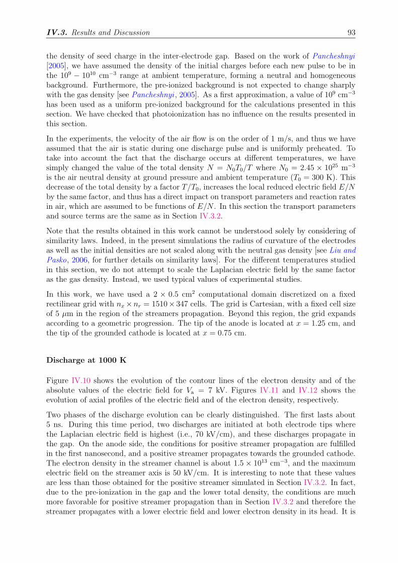
IV.3. Results and Discussion 93
the density of seed charge in the inter-electrode gap. Based on the work of Pancheshnyi[2005], we have assumed the density of the initial charges before each new pulse to be inthe 109 − 1010 cm−3 range at ambient temperature, forming a neutral and homogeneousbackground. Furthermore, the pre-ionized background is not expected to change sharplywith the gas density [see Pancheshnyi , 2005]. As a first approximation, a value of 109 cm−3
has been used as a uniform pre-ionized background for the calculations presented in thissection. We have checked that photoionization has no influence on the results presented inthis section.
In the experiments, the velocity of the air flow is on the order of 1 m/s, and thus we haveassumed that the air is static during one discharge pulse and is uniformly preheated. Totake into account the fact that the discharge occurs at different temperatures, we havesimply changed the value of the total density N = N0T0/T where N0 = 2.45 × 1025 m−3
is the air neutral density at ground pressure and ambient temperature (T0 = 300 K). Thisdecrease of the total density by a factor T/T0, increases the local reduced electric field E/Nby the same factor, and thus has a direct impact on transport parameters and reaction ratesin air, which are assumed to be functions of E/N . In this section the transport parametersand source terms are the same as in Section IV.3.2.
Note that the results obtained in this work cannot be understood solely by considering ofsimilarity laws. Indeed, in the present simulations the radius of curvature of the electrodesas well as the initial densities are not scaled along with the neutral gas density [see Liu andPasko, 2006, for further details on similarity laws]. For the different temperatures studiedin this section, we do not attempt to scale the Laplacian electric field by the same factoras the gas density. Instead, we used typical values of experimental studies.
In this work, we have used a 2 × 0.5 cm2 computational domain discretized on a fixedrectilinear grid with nx ×nr = 1510× 347 cells. The grid is Cartesian, with a fixed cell sizeof 5 µm in the region of the streamers propagation. Beyond this region, the grid expandsaccording to a geometric progression. The tip of the anode is located at x = 1.25 cm, andthe tip of the grounded cathode is located at x = 0.75 cm.
Discharge at 1000 K
Figure IV.10 shows the evolution of the contour lines of the electron density and of theabsolute values of the electric field for Va = 7 kV. Figures IV.11 and IV.12 shows theevolution of axial profiles of the electric field and of the electron density, respectively.
Two phases of the discharge evolution can be clearly distinguished. The first lasts about5 ns. During this time period, two discharges are initiated at both electrode tips wherethe Laplacian electric field is highest (i.e., 70 kV/cm), and these discharges propagate inthe gap. On the anode side, the conditions for positive streamer propagation are fulfilledin the first nanosecond, and a positive streamer propagates towards the grounded cathode.The electron density in the streamer channel is about 1.5 × 1013 cm−3, and the maximumelectric field on the streamer axis is 50 kV/cm. It is interesting to note that these valuesare less than those obtained for the positive streamer simulated in Section IV.3.2. In fact,due to the pre-ionization in the gap and the lower total density, the conditions are muchmore favorable for positive streamer propagation than in Section IV.3.2 and therefore thestreamer propagates with a lower electric field and lower electron density in its head. It is
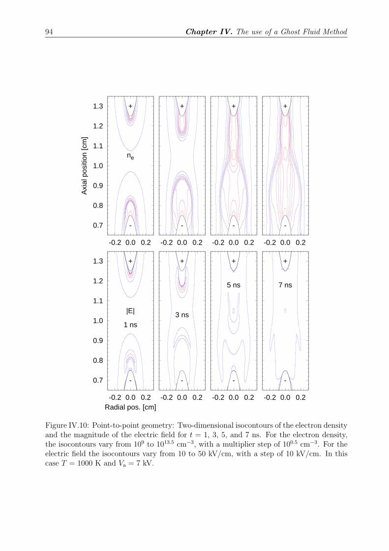
94 Chapter IV. The use of a Ghost Fluid Method
0.7
0.8
0.9
1.0
1.1
1.2
1.3
-0.2 0.0 0.2
Axi
al p
ositi
on [c
m]
ne
1 ns
+
-
-0.2 0.0 0.2
3 ns
+
-
-0.2 0.0 0.2
5 ns
+
-
-0.2 0.0 0.2
7 ns
+
-
0.7
0.8
0.9
1.0
1.1
1.2
1.3
-0.2 0.0 0.2Radial pos. [cm]
|E|
+
-
-0.2 0.0 0.2
+
-
-0.2 0.0 0.2
+
-
-0.2 0.0 0.2
+
-
Figure IV.10: Point-to-point geometry: Two-dimensional isocontours of the electron densityand the magnitude of the electric field for t = 1, 3, 5, and 7 ns. For the electron density,the isocontours vary from 109 to 1013.5 cm−3, with a multiplier step of 100.5 cm−3. For theelectric field the isocontours vary from 10 to 50 kV/cm, with a step of 10 kV/cm. In thiscase T = 1000 K and Va = 7 kV.
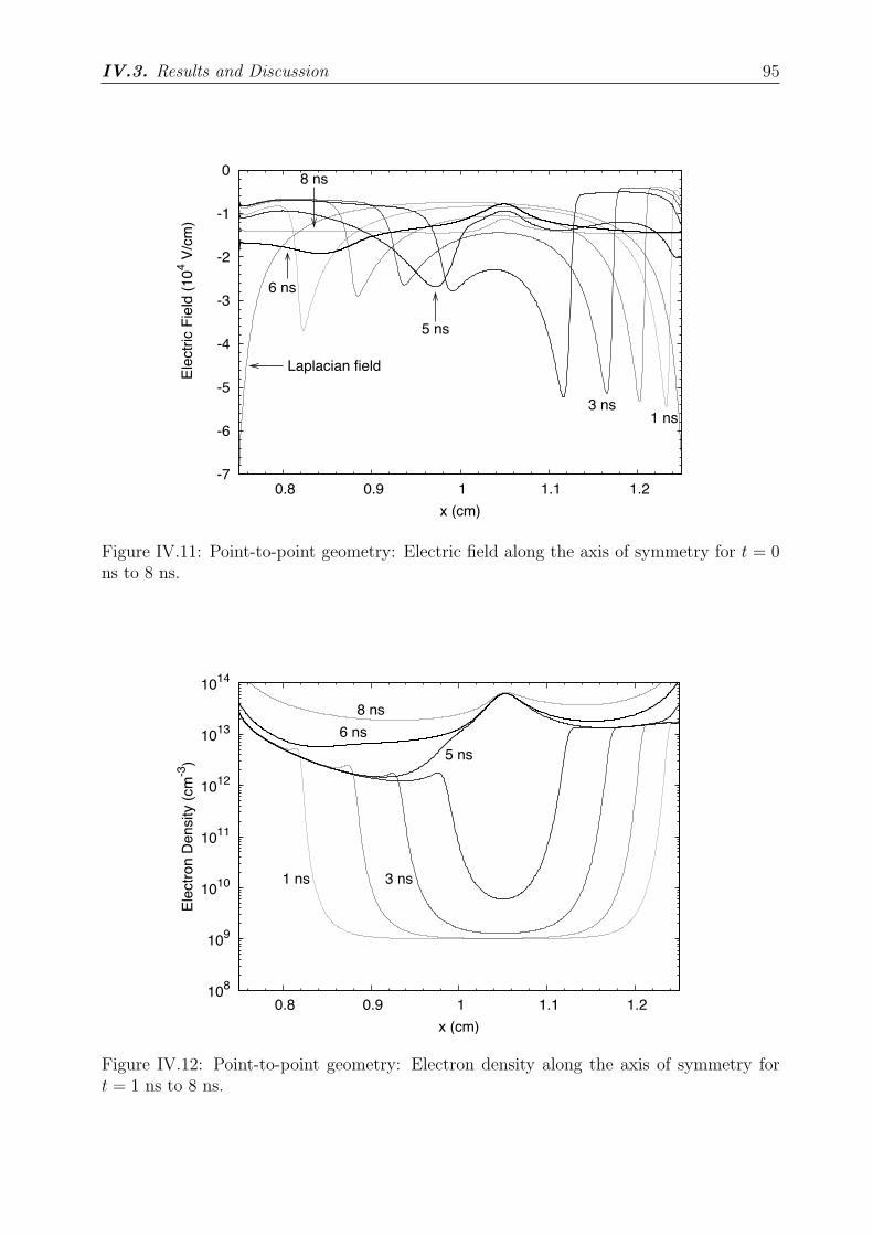
IV.3. Results and Discussion 95
-7
-6
-5
-4
-3
-2
-1
0
0.8 0.9 1 1.1 1.2
x (cm)
Ele
ctr
ic F
ield
(10
4 V
/cm
)
1 ns3 ns
5 ns
6 ns
8 ns
Laplacian field
Figure IV.11: Point-to-point geometry: Electric field along the axis of symmetry for t = 0ns to 8 ns.
108
109
1010
1011
1012
1013
1014
0.8 0.9 1 1.1 1.2
x (cm)
Ele
ctr
on D
ensity (
cm
-3)
1 ns 3 ns
5 ns
6 ns
8 ns
Figure IV.12: Point-to-point geometry: Electron density along the axis of symmetry fort = 1 ns to 8 ns.
96 Chapter IV. The use of a Ghost Fluid Method
interesting to note that Liu and Pasko [2006] have compared streamer propagation at 300K at atmospheric pressure to that at lower pressures. These authors indicated that at lowpressures, the maximum electric field and electron density are less than that at atmosphericpressure. In their work, the change of pressure has a direct impact on the quenching ofthe radiative molecular states responsible for photoionization, and thus the photoionizationsource term decreases as the pressure increases. We note that our results obtained at 1000K with pre-ionization in the gap are close to the results of Liu and Pasko [2006] at lowpressure. However, we note again that in our case the Laplacian electric field and thepre-ionization level are not defined following the similarity laws.
On the cathode side, in the first few nanoseconds we observe the expansion of a dischargetowards the anode. The maximum electric field in the discharge decreases as the dischargepropagates towards the anode and is on the order of 30 kV/cm. The electron density in thedischarge front is on the order of 1012 cm−3. Due to the pre-ionization in the inter-electrodegap, these values are less than those usually obtained for negative streamers [e.g., Bourdonet al., 2007], and we can quantify that the discharge which propagates from the cathodeas a “weak” negative streamer. We also carried out simulations without a continuousionized background, and initializing the streamer by a neutral plasma cloud in the vicinityof the anode (as in Section IV.3.2). In this case we found that the weak negative streameris ignited from the cathode as well, but in this situation the ignition is only due to thephotoionization of the positive streamer instead of the uniform background density.
In Figure IV.10 both discharges have very different radial expansions. At t ≃ 5 ns, bothdischarges interact at z ≃ 1.05 cm, and Figures IV.11 and IV.12 clearly show that thepositive streamer propagates very rapidly towards the cathode in the volume pre-ionizedby the “weak” negative streamer. Then at t = 7 ns the positive streamer reaches thegrounded electrode, and Figure IV.11 shows the rapid redistribution of the potential in theinterelectrode gap. In Figure IV.12, we note that the interaction between the two dischargescreates an enhancement in the electron density at z ≃ 1.05 cm and this enhancementremains nearly unchanged for t > 5 ns. We also note that for t > 5 ns the electron numberdensity increases on the discharge axis.
All these results indicate that a positive streamer could propagate between the two pointelectrodes in less than 7 ns, which is in qualitative agreement with the experimental results.In this case an electrical connection between two electrodes is realized with quite a highelectron density. This junction is created after the positive streamer reaches the cathode.Depending on the temperatures and voltages studied, this connection can form during theapplied-voltage pulse (10 ns long for the experiment considered). As a result, the current inthe conducting junction increases and the plasma filament develops into a spark discharge.
In Figure IV.13, the conditions are the same as in Figure IV.10, except that the appliedvoltage at the anode is Va = 5 kV. As for Figure IV.10, we observe that two discharges areignited in the vicinity of the electrodes, which are of opposit polarity. The results obtainedare similar to the case with Va = 7 kV, but in this case the propagation time scale ofnegative and positive streamers is much longer. The positive streamer contacts the regionionized by the weak negative streamer only after 13.5 ns and finally reaches the cathodeafter 20 ns. The electrical connection is not realized during the 10 ns long voltage pulse,and therefore one expects to obtain only corona discharges on such a time scale.
In the experimental results at 1000 K, corona discharges are present up to Va = 6 kV, and
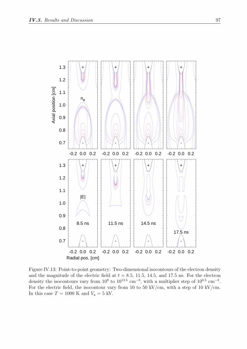
IV.3. Results and Discussion 97
0.7
0.8
0.9
1.0
1.1
1.2
1.3
-0.2 0.0 0.2
Axi
al p
ositi
on [c
m]
ne
8.5 ns
+
-
-0.2 0.0 0.2
11.5 ns
+
-
-0.2 0.0 0.2
14.5 ns
+
-
-0.2 0.0 0.2
17.5 ns
+
-
0.7
0.8
0.9
1.0
1.1
1.2
1.3
-0.2 0.0 0.2Radial pos. [cm]
|E|
+
-
-0.2 0.0 0.2
+
-
-0.2 0.0 0.2
+
-
-0.2 0.0 0.2
+
-
Figure IV.13: Point-to-point geometry: Two-dimensional isocontours of the electron densityand the magnitude of the electric field at t = 8.5, 11.5, 14.5, and 17.5 ns. For the electrondensity the isocontours vary from 109 to 1013.5 cm−3, with a multiplier step of 100.5 cm−3.For the electric field, the isocontour vary from 10 to 50 kV/cm, with a step of 10 kV/cm.In this case T = 1000 K and Va = 5 kV.
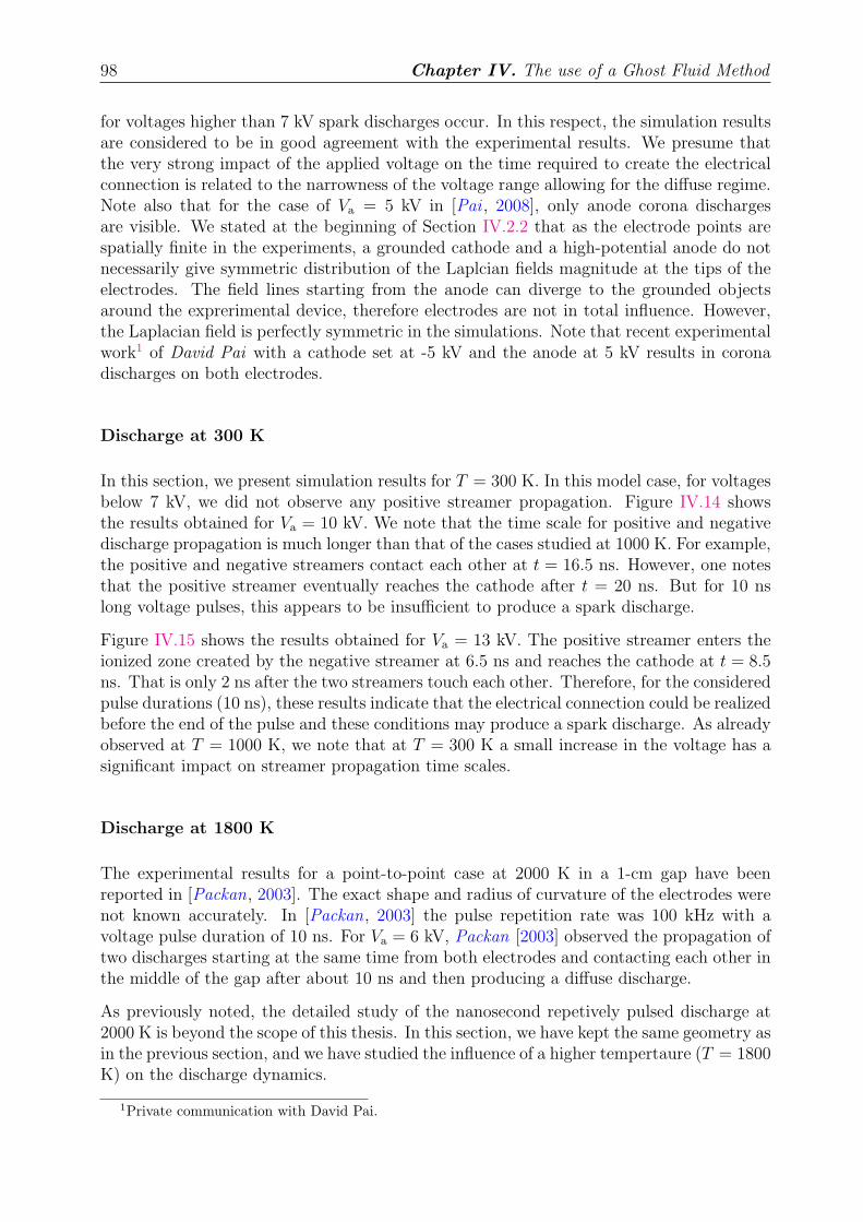
98 Chapter IV. The use of a Ghost Fluid Method
for voltages higher than 7 kV spark discharges occur. In this respect, the simulation resultsare considered to be in good agreement with the experimental results. We presume thatthe very strong impact of the applied voltage on the time required to create the electricalconnection is related to the narrowness of the voltage range allowing for the diffuse regime.Note also that for the case of Va = 5 kV in [Pai , 2008], only anode corona dischargesare visible. We stated at the beginning of Section IV.2.2 that as the electrode points arespatially finite in the experiments, a grounded cathode and a high-potential anode do notnecessarily give symmetric distribution of the Laplcian fields magnitude at the tips of theelectrodes. The field lines starting from the anode can diverge to the grounded objectsaround the exprerimental device, therefore electrodes are not in total influence. However,the Laplacian field is perfectly symmetric in the simulations. Note that recent experimentalwork1 of David Pai with a cathode set at -5 kV and the anode at 5 kV results in coronadischarges on both electrodes.
Discharge at 300 K
In this section, we present simulation results for T = 300 K. In this model case, for voltagesbelow 7 kV, we did not observe any positive streamer propagation. Figure IV.14 showsthe results obtained for Va = 10 kV. We note that the time scale for positive and negativedischarge propagation is much longer than that of the cases studied at 1000 K. For example,the positive and negative streamers contact each other at t = 16.5 ns. However, one notesthat the positive streamer eventually reaches the cathode after t = 20 ns. But for 10 nslong voltage pulses, this appears to be insufficient to produce a spark discharge.
Figure IV.15 shows the results obtained for Va = 13 kV. The positive streamer enters theionized zone created by the negative streamer at 6.5 ns and reaches the cathode at t = 8.5ns. That is only 2 ns after the two streamers touch each other. Therefore, for the consideredpulse durations (10 ns), these results indicate that the electrical connection could be realizedbefore the end of the pulse and these conditions may produce a spark discharge. As alreadyobserved at T = 1000 K, we note that at T = 300 K a small increase in the voltage has asignificant impact on streamer propagation time scales.
Discharge at 1800 K
The experimental results for a point-to-point case at 2000 K in a 1-cm gap have beenreported in [Packan, 2003]. The exact shape and radius of curvature of the electrodes werenot known accurately. In [Packan, 2003] the pulse repetition rate was 100 kHz with avoltage pulse duration of 10 ns. For Va = 6 kV, Packan [2003] observed the propagation oftwo discharges starting at the same time from both electrodes and contacting each other inthe middle of the gap after about 10 ns and then producing a diffuse discharge.
As previously noted, the detailed study of the nanosecond repetively pulsed discharge at2000 K is beyond the scope of this thesis. In this section, we have kept the same geometry asin the previous section, and we have studied the influence of a higher tempertaure (T = 1800K) on the discharge dynamics.
1Private communication with David Pai.
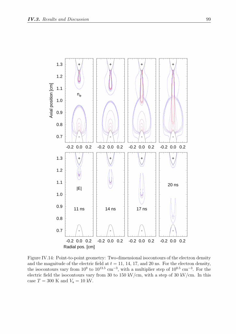
IV.3. Results and Discussion 99
0.7
0.8
0.9
1.0
1.1
1.2
1.3
-0.2 0.0 0.2
Axi
al p
ositi
on [c
m]
ne
11 ns
+
-
-0.2 0.0 0.2
14 ns
+
-
-0.2 0.0 0.2
17 ns
+
-
-0.2 0.0 0.2
20 ns
+
-
0.7
0.8
0.9
1.0
1.1
1.2
1.3
-0.2 0.0 0.2Radial pos. [cm]
|E|
+
-
-0.2 0.0 0.2
+
-
-0.2 0.0 0.2
+
-
-0.2 0.0 0.2
+
-
Figure IV.14: Point-to-point geometry: Two-dimensional isocontours of the electron densityand the magnitude of the electric field at t = 11, 14, 17, and 20 ns. For the electron density,the isocontours vary from 109 to 1013.5 cm−3, with a multiplier step of 100.5 cm−3. For theelectric field the isocontours vary from 30 to 150 kV/cm, with a step of 30 kV/cm. In thiscase T = 300 K and Va = 10 kV.
100 Chapter IV. The use of a Ghost Fluid Method
0.7
0.8
0.9
1.0
1.1
1.2
1.3
-0.2 0.0 0.2
Axi
al p
ositi
on [c
m]
ne
2 ns
+
-
-0.2 0.0 0.2
4 ns
+
-
-0.2 0.0 0.2
6 ns
+
-
-0.2 0.0 0.2
8 ns
+
-
0.7
0.8
0.9
1.0
1.1
1.2
1.3
-0.2 0.0 0.2Radial pos. [cm]
|E|
+
-
-0.2 0.0 0.2
+
-
-0.2 0.0 0.2
+
-
-0.2 0.0 0.2
+
-
Figure IV.15: Point-to-point geometry: Two-dimensional isocontours of the electron densityand the magnitude of the electric field at t = 2, 4, 6, and 8 ns. For the electron densitythe isocontours vary from 109 to 1013.5 cm−3, with a multiplier step of 100.5 cm−3. For theelectric field the isocontours vary from 30 to 150 kV/cm, with a step of 30 kV/cm. In thiscase T = 300 K and Va = 13 kV.
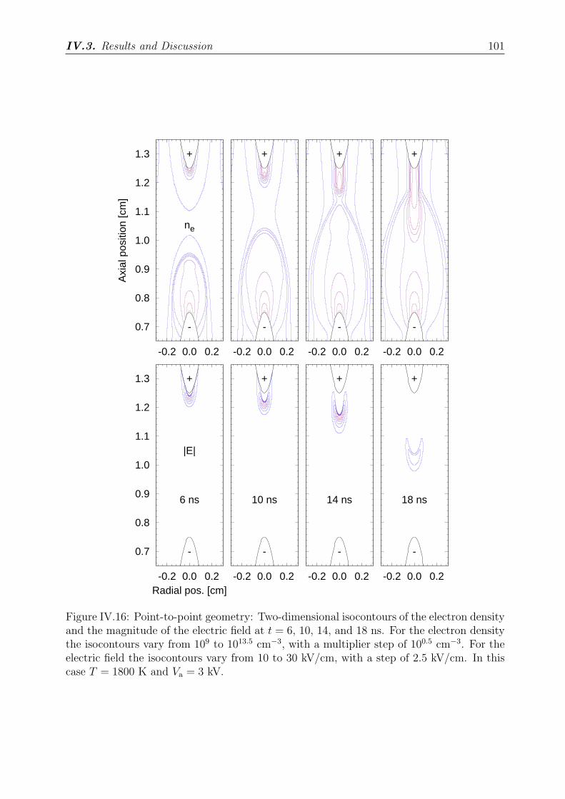
IV.3. Results and Discussion 101
0.7
0.8
0.9
1.0
1.1
1.2
1.3
-0.2 0.0 0.2
Axi
al p
ositi
on [c
m]
ne
6 ns
+
-
-0.2 0.0 0.2
10 ns
+
-
-0.2 0.0 0.2
14 ns
+
-
-0.2 0.0 0.2
18 ns
+
-
0.7
0.8
0.9
1.0
1.1
1.2
1.3
-0.2 0.0 0.2Radial pos. [cm]
|E|
+
-
-0.2 0.0 0.2
+
-
-0.2 0.0 0.2
+
-
-0.2 0.0 0.2
+
-
Figure IV.16: Point-to-point geometry: Two-dimensional isocontours of the electron densityand the magnitude of the electric field at t = 6, 10, 14, and 18 ns. For the electron densitythe isocontours vary from 109 to 1013.5 cm−3, with a multiplier step of 100.5 cm−3. For theelectric field the isocontours vary from 10 to 30 kV/cm, with a step of 2.5 kV/cm. In thiscase T = 1800 K and Va = 3 kV.
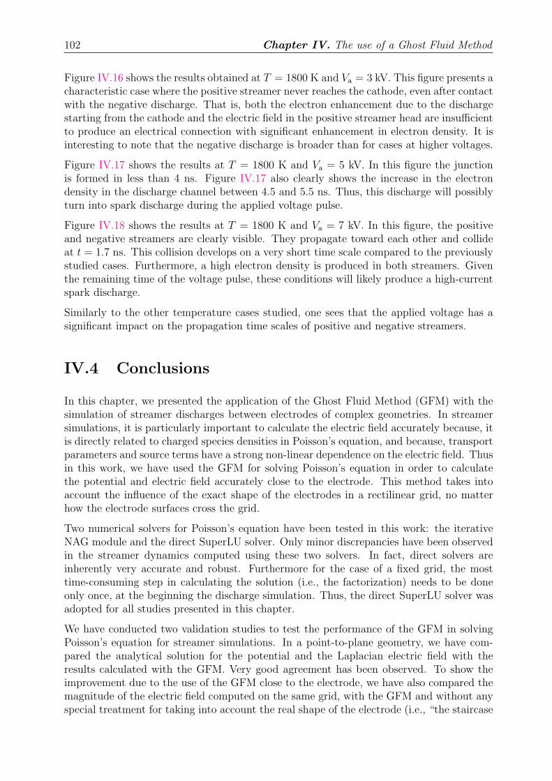
102 Chapter IV. The use of a Ghost Fluid Method
Figure IV.16 shows the results obtained at T = 1800 K and Va = 3 kV. This figure presents acharacteristic case where the positive streamer never reaches the cathode, even after contactwith the negative discharge. That is, both the electron enhancement due to the dischargestarting from the cathode and the electric field in the positive streamer head are insufficientto produce an electrical connection with significant enhancement in electron density. It isinteresting to note that the negative discharge is broader than for cases at higher voltages.
Figure IV.17 shows the results at T = 1800 K and Va = 5 kV. In this figure the junctionis formed in less than 4 ns. Figure IV.17 also clearly shows the increase in the electrondensity in the discharge channel between 4.5 and 5.5 ns. Thus, this discharge will possiblyturn into spark discharge during the applied voltage pulse.
Figure IV.18 shows the results at T = 1800 K and Va = 7 kV. In this figure, the positiveand negative streamers are clearly visible. They propagate toward each other and collideat t = 1.7 ns. This collision develops on a very short time scale compared to the previouslystudied cases. Furthermore, a high electron density is produced in both streamers. Giventhe remaining time of the voltage pulse, these conditions will likely produce a high-currentspark discharge.
Similarly to the other temperature cases studied, one sees that the applied voltage has asignificant impact on the propagation time scales of positive and negative streamers.
IV.4 Conclusions
In this chapter, we presented the application of the Ghost Fluid Method (GFM) with thesimulation of streamer discharges between electrodes of complex geometries. In streamersimulations, it is particularly important to calculate the electric field accurately because, itis directly related to charged species densities in Poisson’s equation, and because, transportparameters and source terms have a strong non-linear dependence on the electric field. Thusin this work, we have used the GFM for solving Poisson’s equation in order to calculatethe potential and electric field accurately close to the electrode. This method takes intoaccount the influence of the exact shape of the electrodes in a rectilinear grid, no matterhow the electrode surfaces cross the grid.
Two numerical solvers for Poisson’s equation have been tested in this work: the iterativeNAG module and the direct SuperLU solver. Only minor discrepancies have been observedin the streamer dynamics computed using these two solvers. In fact, direct solvers areinherently very accurate and robust. Furthermore for the case of a fixed grid, the mosttime-consuming step in calculating the solution (i.e., the factorization) needs to be doneonly once, at the beginning the discharge simulation. Thus, the direct SuperLU solver wasadopted for all studies presented in this chapter.
We have conducted two validation studies to test the performance of the GFM in solvingPoisson’s equation for streamer simulations. In a point-to-plane geometry, we have com-pared the analytical solution for the potential and the Laplacian electric field with theresults calculated with the GFM. Very good agreement has been observed. To show theimprovement due to the use of the GFM close to the electrode, we have also compared themagnitude of the electric field computed on the same grid, with the GFM and without anyspecial treatment for taking into account the real shape of the electrode (i.e., “the staircase
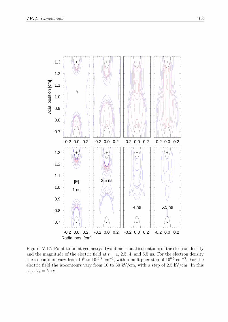
IV.4. Conclusions 103
0.7
0.8
0.9
1.0
1.1
1.2
1.3
-0.2 0.0 0.2
Axi
al p
ositi
on [c
m]
ne
1 ns
+
-
-0.2 0.0 0.2
2.5 ns
+
-
-0.2 0.0 0.2
4 ns
+
-
-0.2 0.0 0.2
5.5 ns
+
-
0.7
0.8
0.9
1.0
1.1
1.2
1.3
-0.2 0.0 0.2Radial pos. [cm]
|E|
+
-
-0.2 0.0 0.2
+
-
-0.2 0.0 0.2
+
-
-0.2 0.0 0.2
+
-
Figure IV.17: Point-to-point geometry: Two-dimensional isocontours of the electron densityand the magnitude of the electric field at t = 1, 2.5, 4, and 5.5 ns. For the electron densitythe isocontours vary from 109 to 1013.5 cm−3, with a multiplier step of 100.5 cm−3. For theelectric field the isocontours vary from 10 to 30 kV/cm, with a step of 2.5 kV/cm. In thiscase Va = 5 kV.
104 Chapter IV. The use of a Ghost Fluid Method
0.7
0.8
0.9
1.0
1.1
1.2
1.3
-0.2 0.0 0.2
Axi
al p
ositi
on [c
m]
ne
0.5 ns
+
-
-0.2 0.0 0.2
1 ns
+
-
-0.2 0.0 0.2
1.5 ns
+
-
-0.2 0.0 0.2
2 ns
+
-
0.7
0.8
0.9
1.0
1.1
1.2
1.3
-0.2 0.0 0.2Radial pos. [cm]
|E|
+
-
-0.2 0.0 0.2
+
-
-0.2 0.0 0.2
+
-
-0.2 0.0 0.2
+
-
Figure IV.18: Point-to-point geometry: Two-dimensional isocontours of the electron densityand the magnitude of the electric field at t = 0.5, 1, 1.5, and 2 ns. For the electron densitythe isocontours vary from 109 to 1013.5 cm−3, with a multiplier step of 100.5 cm−3. For theelectric field the isocontours vary from 10 to 30 kV/cm, with a step of 2.5 kV/cm. In thiscase Va = 7 kV.
IV.4. Conclusions 105
approach”). As expected, the discrepancy between the two numerical approaches increasesas the grid becomes coarser. We have also shown that without the GFM, the electric fieldalong the electrode surface may present unphysical oscillations due to the random crossingof the electrode surface with the grid. Second, we have compared results obtained using theGFM with results obtained by Kulikovsky [1998] for the simulation of the positive streamerpropagation in a hyperboloid-to-plane configuration. Good agreement has been obtainedon all positive streamer characteristics during its propagation in the interelectrode gap.Finally, we have applied the GFM to simulate the discharge in preheated air (at 1000 K)at atmospheric pressure in point-to-point geometry (with a 5 mm interelectrode gap). Thisdischarge has been studied experimentally in [Pai et al., 2008; Pai , 2008]. For a constantapplied voltage of 7 kV, we have shown that positive and negative streamers start to prop-agate in the gap from the anode and cathode, respectively. After the streamer interact inthe gap, we have observed a very rapid propagation of the positive streamer towards thecathode in the volume pre-ionized by the negative streamer. This structure of the dischargeis in qualitative agreement with the experiments.
To take a first step towards understanding of the structure of discharges in point-to-pointgeometry in preheated air, we have carried out a short comparison study for several tem-peratures and applied voltages. Considering propagation time scale of the positive streamermake possible to draw conclusions about the final discharge structure (i.e., spark dischargesor corona discharges) that are in good agreement with the experiments. This also indicatesthat the streamer modeling at short time scales can be of a great help for the understand-ing of nano-pulsed discharges at atmospheric pressure. In particular, it could indicate onthe key physical mechanisms leading to the diffuse regime (“D” regime) and the ranges ofparameters needed for generating this regime at atmospheric pressure. However, this studyis only a first step towards a more thorough comparison study between experiment andsimulation.
In this work, we have shown that the GFM is a simple method which can be readily imple-mented in existing discharge codes. In this chapter, we have studied discharges propagatingbetween metallic electrodes, but the GFM can be easily extended to simulate dielectric bar-rier discharges in complex two- and three-dimensional geometries, or to study the influenceof obstacles (i.e., dust particles, droplets, etc) on the streamer propagation.
In this work, no special numerical treatment has been done close to the needle electrodesto take into account the exact shape of the electrode in setting up boundary conditionsfor drift-diffusion equations of charged species. The boundary conditions are computed inboth directions on the grid assuming that the interface has a “staircase” shape. In thischapter, as in [Kulikovsky , 1997a], we have used simplified boundary conditions: near theanode and cathode surfaces, the gradient of the electron density is taken to be equal to zero.More realistic boundary conditions for electrodes with complex geometries (i.e., secondaryemission processes due to ion bombardment, photoemission, etc), require modeling thereal shape of the electrode for setting up boundary conditions of drift-diffusion equations ofcharged species. For flows in complex geometries, Tseng and Ferziger [2003] have developedthe ghost-cell immersed boundary method (GCIBM). This method handles Dirichlet andNeumann boundary conditions while preserving the overall second-order accuracy of thesolver that they use in the flow far from boundaries. In [Zeghondy et al., 2007], we haveapplied the GCIBM to implement Neumann boundary conditions on a hyperboloid anodein a point-to-plane geometry.

Chapter V
Experimental study of the impact ofa dielectric material on thefilamentary discharges
Table of ContentsV.1 Introduction . . . . . . . . . . . . . . . . . . . . . . . . . . . . . . 108
V.2 Experimental setup . . . . . . . . . . . . . . . . . . . . . . . . . . 109
V.2.1 DBD reactor . . . . . . . . . . . . . . . . . . . . . . . . . . . . . 109
V.2.2 Electrical diagnostics . . . . . . . . . . . . . . . . . . . . . . . . . 110
V.2.3 Current measurement and charge transfer . . . . . . . . . . . . . 112
V.2.4 Injected power . . . . . . . . . . . . . . . . . . . . . . . . . . . . 113
V.3 Current peak statistics . . . . . . . . . . . . . . . . . . . . . . . . 113
V.3.1 Temporal occurrence of current peaks . . . . . . . . . . . . . . . 113
V.3.2 Number of current peaks per half-cycle . . . . . . . . . . . . . . 114
V.3.3 Influence of first event on subsequent events . . . . . . . . . . . . 115
V.4 CCD imaging of individual current peaks during the positivehalf-cycle . . . . . . . . . . . . . . . . . . . . . . . . . . . . . . . . 116
V.4.1 Methodology . . . . . . . . . . . . . . . . . . . . . . . . . . . . . 116
V.4.2 Imaging results . . . . . . . . . . . . . . . . . . . . . . . . . . . . 117
Images of a ‘first current peak’ . . . . . . . . . . . . . . . . . . . 118
Images of a ‘second current peak’ . . . . . . . . . . . . . . . . . . 118
V.4.3 Spatial and temporal self-organization relation between filamentlength and ignition voltage of a current peak . . . . . . . . . . . 119
V.5 Electrostatic modeling . . . . . . . . . . . . . . . . . . . . . . . . 120
V.6 Discussion . . . . . . . . . . . . . . . . . . . . . . . . . . . . . . . . 122
V.7 Conclusions . . . . . . . . . . . . . . . . . . . . . . . . . . . . . . . 124
108 Chapter V. Experimental study of the filamentary discharges in a DBD
As a clear example of the strong influence a dielectric material on the filamentary dis-charges, we experimentally studied a specific Dielectric Barrier Discharge (DBD) configu-ration. Some results of this chapter have been published in [Celestin et al., 2008b].
V.1 Introduction
Dielectric barrier discharges (DBDs), also known as barrier discharges or silent dis-charges, have been studied since the invention of the ozonizer by Siemens in 1857.
Nowadays DBDs are widely used for industrial applications [Eliasson and Kogelschatz ,1991a], such as gas depollution, surface treatment, excimer lamps, ozone generation andplasma display panels. At atmospheric pressure (for gaseous gaps on the order of a fewmillimeters), DBDs are mainly constituted of unstably triggered non-equilibrium transientplasma filaments (also called microdischarges) [Eliasson and Kogelschatz , 1991a]. The shortduration (a few tens of nanoseconds) and unpredictable triggering of these filaments makethem difficult to study experimentally. During the last decade, a few authors have succeededin following the propagation of a single filament (the streamer phase) with high resolutionin time and space in a double dielectric barrier configuration, and thus have determinedthe electron density and electric field inside using spectroscopic diagnostics [Kozlov et al.,2001].
Guikema et al. [2000] observed self-organized patterns in a one-dimensional symmetricDBD system with He/Ar mixtures and associated the patterns with characteristics forcharge transfer during one cycle of the applied voltage (for frequencies on the order of a fewkilohertz). They concluded that the patterns resulted from the presence of surface chargedeposits; that is, related to the intrinsic so-called memory effect of DBDs [e.g., Eliassonand Kogelschatz , 1991a; Golubovskii et al., 2002]. Klein et al. [2001] progressed furtherin this study by improving the time resolution of the imaging technique and observedthat the patterns obtained in [Guikema et al., 2000] were in fact constituted of severalfilaments ignited at different times, which were spatially and temporally controlled bythe residual surface charges on the dielectric. It is also interesting to note that Chirokovet al. [2004] also demonstrated a behavior of self-organization in a plane-to-plane DBD inair at atmospheric pressure driven by high-frequency sinusoidal voltage (kHz) through acomparison of experimental results with a numerical model.
Recently, Guaitella et al. [2006] described the bimodal behavior of the statistical distributionof current peaks in a cylindrical DBD, and they concluded that the high-current group wasdue to the self-triggering of several filaments, presumably correlated by a radiative effectcalled the collective effect. They also studied the impact of this collective effect on theinjected energy in the discharge, which directly controls the chemistry. Collective behaviorof microdischarges has also been recently observed by imaging with a CCD camera on
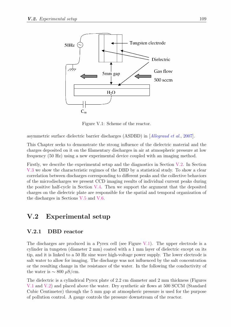
V.2. Experimental setup 109
Figure V.1: Scheme of the reactor.
asymmetric surface dielectric barrier discharges (ASDBD) in [Allegraud et al., 2007].
This Chapter seeks to demonstrate the strong influence of the dielectric material and thecharges deposited on it on the filamentary discharges in air at atmospheric pressure at lowfrequency (50 Hz) using a new experimental device coupled with an imaging method.
Firstly, we describe the experimental setup and the diagnostics in Section V.2. In SectionV.3 we show the characteristic regimes of the DBD by a statistical study. To show a clearcorrelation between discharges corresponding to different peaks and the collective behaviorsof the microdischarges we present CCD imaging results of individual current peaks duringthe positive half-cycle in Section V.4. Then we support the argument that the depositedcharges on the dielectric plate are responsible for the spatial and temporal organization ofthe discharges in Sections V.5 and V.6.
V.2 Experimental setup
V.2.1 DBD reactor
The discharges are produced in a Pyrex cell (see Figure V.1). The upper electrode is acylinder in tungsten (diameter 2 mm) coated with a 1 mm layer of dielectric except on itstip, and it is linked to a 50 Hz sine wave high-voltage power supply. The lower electrode issalt water to allow for imaging. The discharge was not influenced by the salt concentrationor the resulting change in the resistance of the water. In the following the conductivity ofthe water is ∼ 800 µS/cm.
The dielectric is a cylindrical Pyrex plate of 2.2 cm diameter and 2 mm thickness (FiguresV.1 and V.2) and placed above the water. Dry synthetic air flows at 500 SCCM (StandardCubic Centimeter) through the 5 mm gap at atmospheric pressure is used for the purposeof pollution control. A gauge controls the pressure downstream of the reactor.
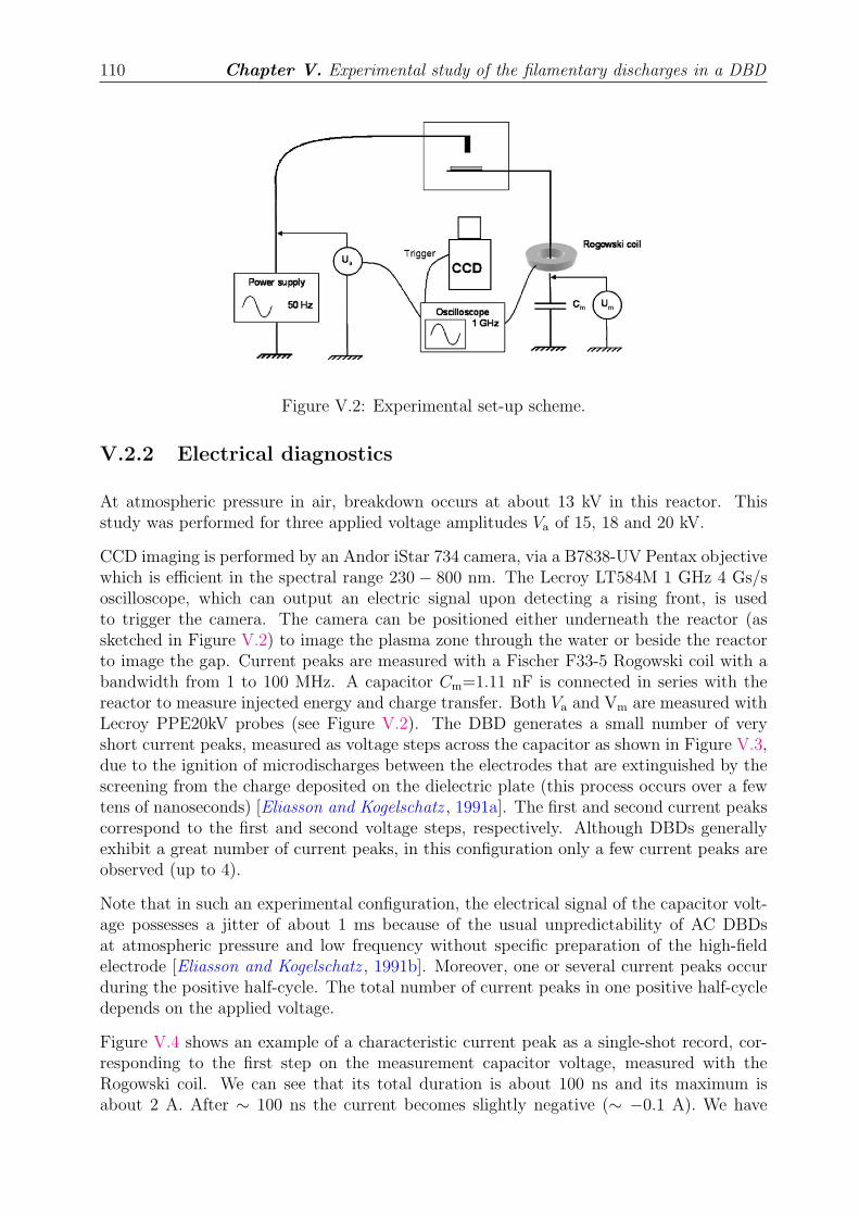
110 Chapter V. Experimental study of the filamentary discharges in a DBD
Figure V.2: Experimental set-up scheme.
V.2.2 Electrical diagnostics
At atmospheric pressure in air, breakdown occurs at about 13 kV in this reactor. Thisstudy was performed for three applied voltage amplitudes Va of 15, 18 and 20 kV.
CCD imaging is performed by an Andor iStar 734 camera, via a B7838-UV Pentax objectivewhich is efficient in the spectral range 230 − 800 nm. The Lecroy LT584M 1 GHz 4 Gs/soscilloscope, which can output an electric signal upon detecting a rising front, is usedto trigger the camera. The camera can be positioned either underneath the reactor (assketched in Figure V.2) to image the plasma zone through the water or beside the reactorto image the gap. Current peaks are measured with a Fischer F33-5 Rogowski coil with abandwidth from 1 to 100 MHz. A capacitor Cm=1.11 nF is connected in series with thereactor to measure injected energy and charge transfer. Both Va and Vm are measured withLecroy PPE20kV probes (see Figure V.2). The DBD generates a small number of veryshort current peaks, measured as voltage steps across the capacitor as shown in Figure V.3,due to the ignition of microdischarges between the electrodes that are extinguished by thescreening from the charge deposited on the dielectric plate (this process occurs over a fewtens of nanoseconds) [Eliasson and Kogelschatz , 1991a]. The first and second current peakscorrespond to the first and second voltage steps, respectively. Although DBDs generallyexhibit a great number of current peaks, in this configuration only a few current peaks areobserved (up to 4).
Note that in such an experimental configuration, the electrical signal of the capacitor volt-age possesses a jitter of about 1 ms because of the usual unpredictability of AC DBDsat atmospheric pressure and low frequency without specific preparation of the high-fieldelectrode [Eliasson and Kogelschatz , 1991b]. Moreover, one or several current peaks occurduring the positive half-cycle. The total number of current peaks in one positive half-cycledepends on the applied voltage.
Figure V.4 shows an example of a characteristic current peak as a single-shot record, cor-responding to the first step on the measurement capacitor voltage, measured with theRogowski coil. We can see that its total duration is about 100 ns and its maximum isabout 2 A. After ∼ 100 ns the current becomes slightly negative (∼ −0.1 A). We have
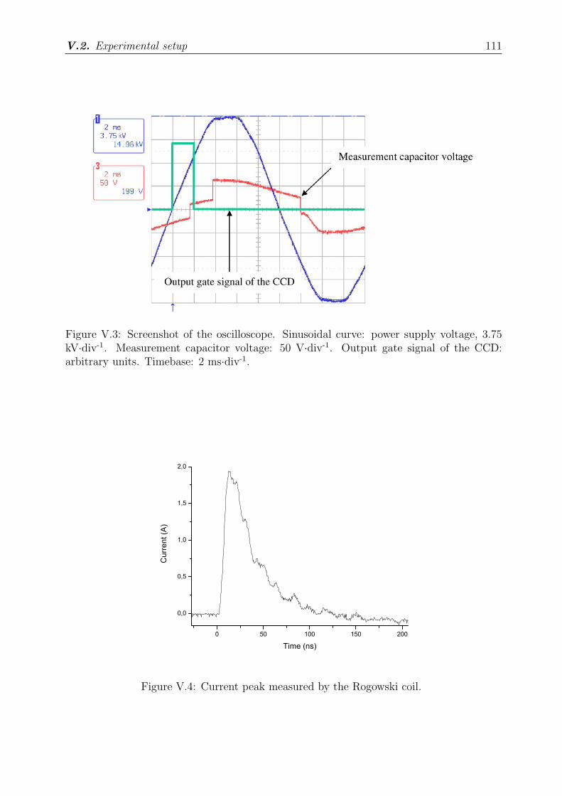
V.2. Experimental setup 111
Figure V.3: Screenshot of the oscilloscope. Sinusoidal curve: power supply voltage, 3.75kV·div-1. Measurement capacitor voltage: 50 V·div-1. Output gate signal of the CCD:arbitrary units. Timebase: 2 ms·div-1.
0 50 100 150 200
0,0
0,5
1,0
1,5
2,0
Cu
rre
nt (A
)
Time (ns)
Figure V.4: Current peak measured by the Rogowski coil.
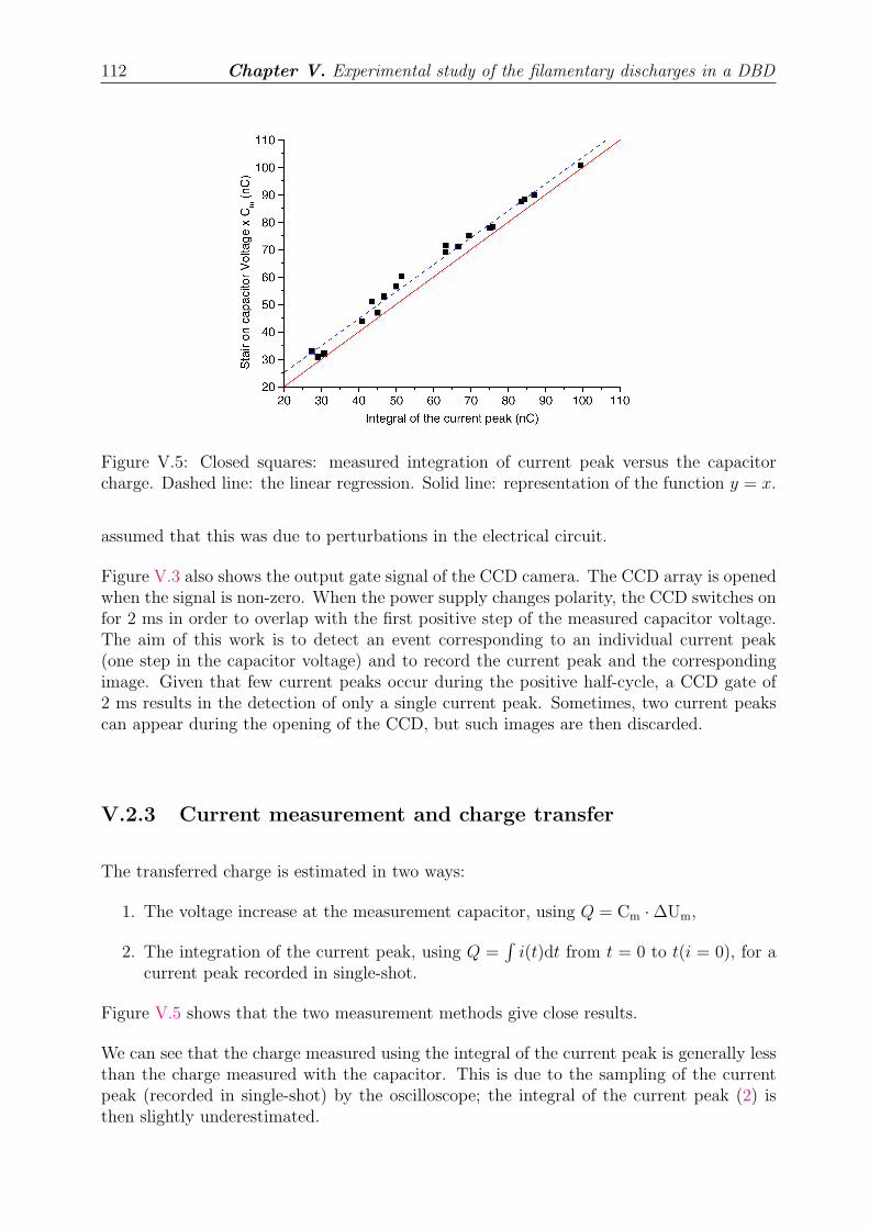
112 Chapter V. Experimental study of the filamentary discharges in a DBD
Figure V.5: Closed squares: measured integration of current peak versus the capacitorcharge. Dashed line: the linear regression. Solid line: representation of the function y = x.
assumed that this was due to perturbations in the electrical circuit.
Figure V.3 also shows the output gate signal of the CCD camera. The CCD array is openedwhen the signal is non-zero. When the power supply changes polarity, the CCD switches onfor 2 ms in order to overlap with the first positive step of the measured capacitor voltage.The aim of this work is to detect an event corresponding to an individual current peak(one step in the capacitor voltage) and to record the current peak and the correspondingimage. Given that few current peaks occur during the positive half-cycle, a CCD gate of2 ms results in the detection of only a single current peak. Sometimes, two current peakscan appear during the opening of the CCD, but such images are then discarded.
V.2.3 Current measurement and charge transfer
The transferred charge is estimated in two ways:
1. The voltage increase at the measurement capacitor, using Q = Cm · ∆Um,
2. The integration of the current peak, using Q =∫
i(t)dt from t = 0 to t(i = 0), for acurrent peak recorded in single-shot.
Figure V.5 shows that the two measurement methods give close results.
We can see that the charge measured using the integral of the current peak is generally lessthan the charge measured with the capacitor. This is due to the sampling of the currentpeak (recorded in single-shot) by the oscilloscope; the integral of the current peak (2) isthen slightly underestimated.
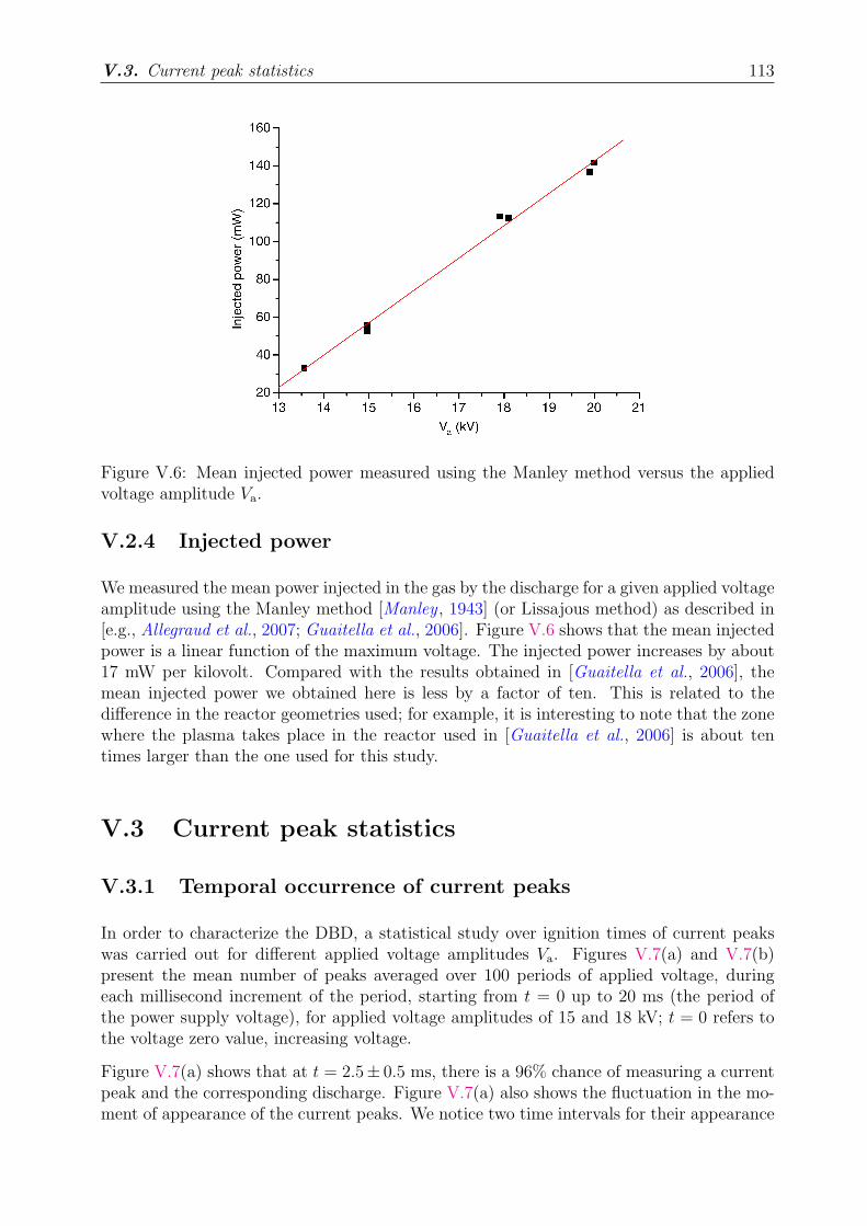
V.3. Current peak statistics 113
Figure V.6: Mean injected power measured using the Manley method versus the appliedvoltage amplitude Va.
V.2.4 Injected power
We measured the mean power injected in the gas by the discharge for a given applied voltageamplitude using the Manley method [Manley , 1943] (or Lissajous method) as described in[e.g., Allegraud et al., 2007; Guaitella et al., 2006]. Figure V.6 shows that the mean injectedpower is a linear function of the maximum voltage. The injected power increases by about17 mW per kilovolt. Compared with the results obtained in [Guaitella et al., 2006], themean injected power we obtained here is less by a factor of ten. This is related to thedifference in the reactor geometries used; for example, it is interesting to note that the zonewhere the plasma takes place in the reactor used in [Guaitella et al., 2006] is about tentimes larger than the one used for this study.
V.3 Current peak statistics
V.3.1 Temporal occurrence of current peaks
In order to characterize the DBD, a statistical study over ignition times of current peakswas carried out for different applied voltage amplitudes Va. Figures V.7(a) and V.7(b)present the mean number of peaks averaged over 100 periods of applied voltage, duringeach millisecond increment of the period, starting from t = 0 up to 20 ms (the period ofthe power supply voltage), for applied voltage amplitudes of 15 and 18 kV; t = 0 refers tothe voltage zero value, increasing voltage.
Figure V.7(a) shows that at t = 2.5± 0.5 ms, there is a 96% chance of measuring a currentpeak and the corresponding discharge. Figure V.7(a) also shows the fluctuation in the mo-ment of appearance of the current peaks. We notice two time intervals for their appearance
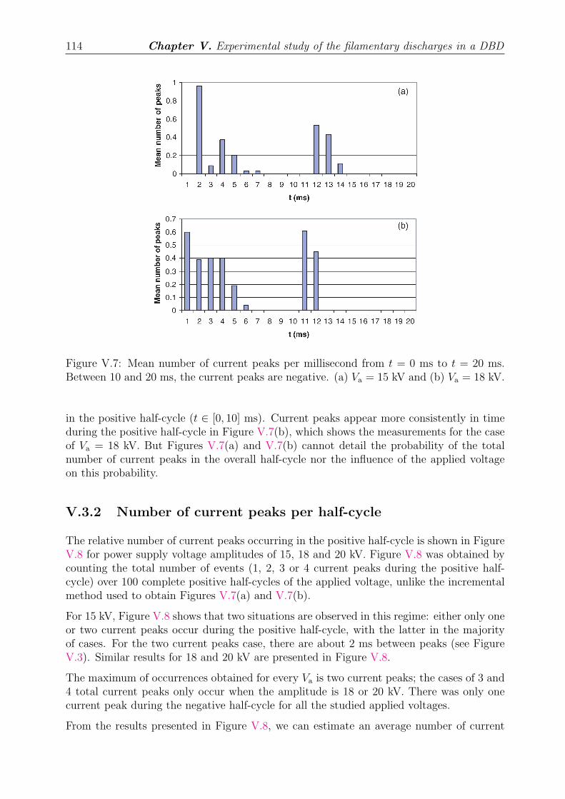
114 Chapter V. Experimental study of the filamentary discharges in a DBD
Figure V.7: Mean number of current peaks per millisecond from t = 0 ms to t = 20 ms.Between 10 and 20 ms, the current peaks are negative. (a) Va = 15 kV and (b) Va = 18 kV.
in the positive half-cycle (t ∈ [0, 10] ms). Current peaks appear more consistently in timeduring the positive half-cycle in Figure V.7(b), which shows the measurements for the caseof Va = 18 kV. But Figures V.7(a) and V.7(b) cannot detail the probability of the totalnumber of current peaks in the overall half-cycle nor the influence of the applied voltageon this probability.
V.3.2 Number of current peaks per half-cycle
The relative number of current peaks occurring in the positive half-cycle is shown in FigureV.8 for power supply voltage amplitudes of 15, 18 and 20 kV. Figure V.8 was obtained bycounting the total number of events (1, 2, 3 or 4 current peaks during the positive half-cycle) over 100 complete positive half-cycles of the applied voltage, unlike the incrementalmethod used to obtain Figures V.7(a) and V.7(b).
For 15 kV, Figure V.8 shows that two situations are observed in this regime: either only oneor two current peaks occur during the positive half-cycle, with the latter in the majorityof cases. For the two current peaks case, there are about 2 ms between peaks (see FigureV.3). Similar results for 18 and 20 kV are presented in Figure V.8.
The maximum of occurrences obtained for every Va is two current peaks; the cases of 3 and4 total current peaks only occur when the amplitude is 18 or 20 kV. There was only onecurrent peak during the negative half-cycle for all the studied applied voltages.
From the results presented in Figure V.8, we can estimate an average number of current

V.3. Current peak statistics 115
Figure V.8: Number of observed total current peaks by percentage during the positivehalf-cycle for a power supply voltage amplitudes of 15, 18 and 20 kV.
Table V.1: Average total number of current peaks during the positive half-cycle.
Va(kV) 15 18 20〈N〉 1.6 2.2 2.4
peaks during the positive half-cycle for each applied voltage amplitude (see Table V.1). Thedata are consistent although insufficient to evaluate a real tendency. Indeed, as expectedfor a DBD, the number of events increases with the applied voltage amplitude. One canestimate a “statistical error” by summing the probabilities obtained in Figures V.7(a) andV.7(b) and dividing by the average total number of peaks. For 15 and 18 kV the errorbars are shown in Figure V.8. These error bars are small (less than 10%) and show theconsistency of the statistical approach used in Figures V.7 and V.8.
V.3.3 Influence of first event on subsequent events
The measured current amplitude of first current peaks during the positive half-cycle whenVa is 18 kV is plotted as a function of Vpeak, the ignition voltage of a first current peak,in Figure V.9. The accuracy of the maximum of a current peak depends on the samplingrate of the current peak by the oscilloscope. Error bars are then evaluated according tothe sampling rate. Higher sampling rates result in smaller error, but lower sampling ratespermit a larger time range.
One can clearly see from Figure V.9 that the maximum of first current peak increases with
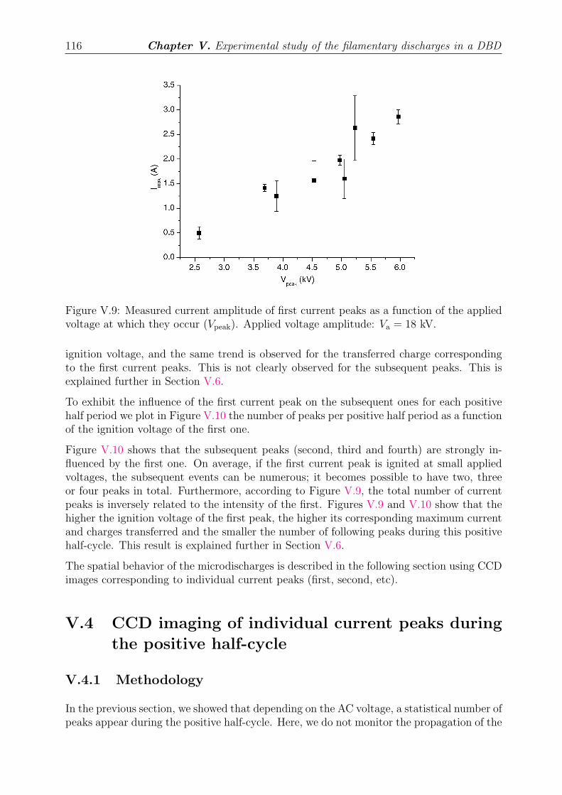
116 Chapter V. Experimental study of the filamentary discharges in a DBD
Figure V.9: Measured current amplitude of first current peaks as a function of the appliedvoltage at which they occur (Vpeak). Applied voltage amplitude: Va = 18 kV.
ignition voltage, and the same trend is observed for the transferred charge correspondingto the first current peaks. This is not clearly observed for the subsequent peaks. This isexplained further in Section V.6.
To exhibit the influence of the first current peak on the subsequent ones for each positivehalf period we plot in Figure V.10 the number of peaks per positive half period as a functionof the ignition voltage of the first one.
Figure V.10 shows that the subsequent peaks (second, third and fourth) are strongly in-fluenced by the first one. On average, if the first current peak is ignited at small appliedvoltages, the subsequent events can be numerous; it becomes possible to have two, threeor four peaks in total. Furthermore, according to Figure V.9, the total number of currentpeaks is inversely related to the intensity of the first. Figures V.9 and V.10 show that thehigher the ignition voltage of the first peak, the higher its corresponding maximum currentand charges transferred and the smaller the number of following peaks during this positivehalf-cycle. This result is explained further in Section V.6.
The spatial behavior of the microdischarges is described in the following section using CCDimages corresponding to individual current peaks (first, second, etc).
V.4 CCD imaging of individual current peaks duringthe positive half-cycle
V.4.1 Methodology
In the previous section, we showed that depending on the AC voltage, a statistical number ofpeaks appear during the positive half-cycle. Here, we do not monitor the propagation of the
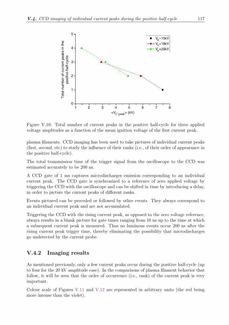
V.4. CCD imaging of individual current peaks during the positive half-cycle 117
Figure V.10: Total number of current peaks in the positive half-cycle for three appliedvoltage amplitudes as a function of the mean ignition voltage of the first current peak.
plasma filaments. CCD imaging has been used to take pictures of individual current peaks(first, second, etc) to study the influence of their ranks (i.e., of their order of appearance inthe positive half-cycle).
The total transmission time of the trigger signal from the oscilloscope to the CCD wasestimated accurately to be 200 ns.
A CCD gate of 1 ms captures microdischarges emission corresponding to an individualcurrent peak. The CCD gate is synchronized to a reference of zero applied voltage bytriggering the CCD with the oscilloscope and can be shifted in time by introducing a delay,in order to picture the current peaks of different ranks.
Events pictured can be preceded or followed by other events. They always correspond toan individual current peak and are not accumulated.
Triggering the CCD with the rising current peak, as opposed to the zero voltage reference,always results in a blank picture for gate times ranging from 10 ns up to the time at whicha subsequent current peak is measured. Thus no luminous events occur 200 ns after therising current peak trigger time, thereby eliminating the possibility that microdischargesgo undetected by the current probe.
V.4.2 Imaging results
As mentioned previously, only a few current peaks occur during the positive half-cycle (upto four for the 20 kV amplitude case). In the comparisons of plasma filament behavior thatfollow, it will be seen that the order of occurrence (i.e., rank) of the current peak is veryimportant.
Colour scale of Figures V.11 and V.12 are represented in arbitrary units (the red beingmore intense than the violet).
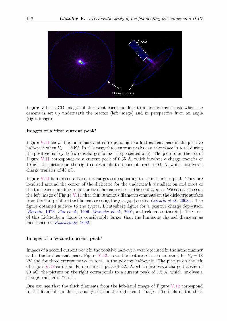
118 Chapter V. Experimental study of the filamentary discharges in a DBD
Figure V.11: CCD images of the event corresponding to a first current peak when thecamera is set up underneath the reactor (left image) and in perspective from an angle(right image).
Images of a ‘first current peak’
Figure V.11 shows the luminous event corresponding to a first current peak in the positivehalf-cycle when Va = 18 kV. In this case, three current peaks can take place in total duringthe positive half-cycle (two discharges follow the presented one). The picture on the left ofFigure V.11 corresponds to a current peak of 0.35 A, which involves a charge transfer of10 nC; the picture on the right corresponds to a current peak of 0.9 A, which involves acharge transfer of 45 nC.
Figure V.11 is representative of discharges corresponding to a first current peak. They arelocalized around the center of the dielectric for the underneath visualization and most ofthe time corresponding to one or two filaments close to the central axis. We can also see onthe left image of Figure V.11 that thin luminous filaments emanate on the dielectric surfacefrom the ‘footprint’ of the filament crossing the gas gap [see also Celestin et al., 2008a]. Thefigure obtained is close to the typical Lichtenberg figure for a positive charge deposition[Bertein, 1973; Zhu et al., 1996; Murooka et al., 2001, and references therein]. The areaof this Lichtenberg figure is considerably larger than the luminous channel diameter asmentioned in [Kogelschatz , 2002].
Images of a ‘second current peak’
Images of a second current peak in the positive half-cycle were obtained in the same manneras for the first current peak. Figure V.12 shows the features of such an event, for Va = 18kV and for three current peaks in total in the positive half-cycle. The picture on the leftof Figure V.12 corresponds to a current peak of 2.25 A, which involves a charge transfer of90 nC; the picture on the right corresponds to a current peak of 1.5 A, which involves acharge transfer of 76 nC.
One can see that the thick filaments from the left-hand image of Figure V.12 correspondto the filaments in the gaseous gap from the right-hand image. The ends of the thick
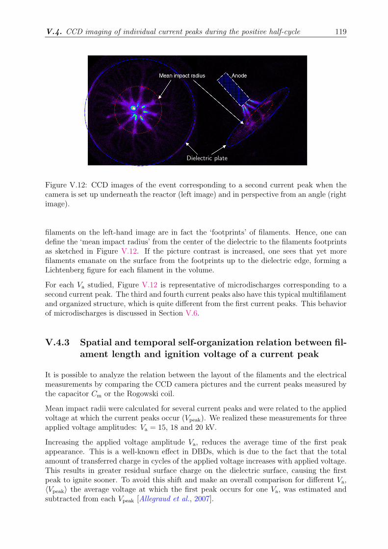
V.4. CCD imaging of individual current peaks during the positive half-cycle 119
Figure V.12: CCD images of the event corresponding to a second current peak when thecamera is set up underneath the reactor (left image) and in perspective from an angle (rightimage).
Dielectric plate
filaments on the left-hand image are in fact the ‘footprints’ of filaments. Hence, one candefine the ‘mean impact radius’ from the center of the dielectric to the filaments footprintsas sketched in Figure V.12. If the picture contrast is increased, one sees that yet morefilaments emanate on the surface from the footprints up to the dielectric edge, forming aLichtenberg figure for each filament in the volume.
For each Va studied, Figure V.12 is representative of microdischarges corresponding to asecond current peak. The third and fourth current peaks also have this typical multifilamentand organized structure, which is quite different from the first current peaks. This behaviorof microdischarges is discussed in Section V.6.
V.4.3 Spatial and temporal self-organization relation between fil-ament length and ignition voltage of a current peak
It is possible to analyze the relation between the layout of the filaments and the electricalmeasurements by comparing the CCD camera pictures and the current peaks measured bythe capacitor Cm or the Rogowski coil.
Mean impact radii were calculated for several current peaks and were related to the appliedvoltage at which the current peaks occur (Vpeak). We realized these measurements for threeapplied voltage amplitudes: Va = 15, 18 and 20 kV.
Increasing the applied voltage amplitude Va, reduces the average time of the first peakappearance. This is a well-known effect in DBDs, which is due to the fact that the totalamount of transferred charge in cycles of the applied voltage increases with applied voltage.This results in greater residual surface charge on the dielectric surface, causing the firstpeak to ignite sooner. To avoid this shift and make an overall comparison for different Va,〈Vpeak〉 the average voltage at which the first peak occurs for one Va, was estimated andsubtracted from each Vpeak [Allegraud et al., 2007].
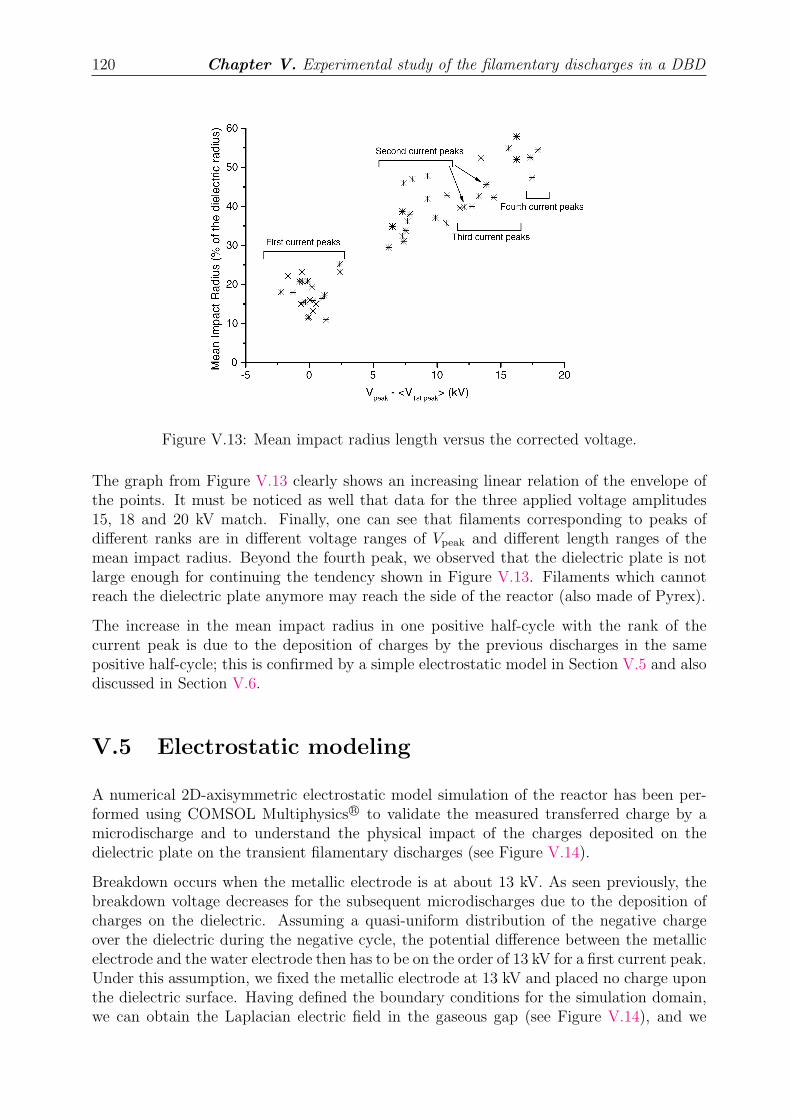
120 Chapter V. Experimental study of the filamentary discharges in a DBD
Figure V.13: Mean impact radius length versus the corrected voltage.
The graph from Figure V.13 clearly shows an increasing linear relation of the envelope ofthe points. It must be noticed as well that data for the three applied voltage amplitudes15, 18 and 20 kV match. Finally, one can see that filaments corresponding to peaks ofdifferent ranks are in different voltage ranges of Vpeak and different length ranges of themean impact radius. Beyond the fourth peak, we observed that the dielectric plate is notlarge enough for continuing the tendency shown in Figure V.13. Filaments which cannotreach the dielectric plate anymore may reach the side of the reactor (also made of Pyrex).
The increase in the mean impact radius in one positive half-cycle with the rank of thecurrent peak is due to the deposition of charges by the previous discharges in the samepositive half-cycle; this is confirmed by a simple electrostatic model in Section V.5 and alsodiscussed in Section V.6.
V.5 Electrostatic modeling
A numerical 2D-axisymmetric electrostatic model simulation of the reactor has been per-formed using COMSOL Multiphysics R© to validate the measured transferred charge by amicrodischarge and to understand the physical impact of the charges deposited on thedielectric plate on the transient filamentary discharges (see Figure V.14).
Breakdown occurs when the metallic electrode is at about 13 kV. As seen previously, thebreakdown voltage decreases for the subsequent microdischarges due to the deposition ofcharges on the dielectric. Assuming a quasi-uniform distribution of the negative chargeover the dielectric during the negative cycle, the potential difference between the metallicelectrode and the water electrode then has to be on the order of 13 kV for a first current peak.Under this assumption, we fixed the metallic electrode at 13 kV and placed no charge uponthe dielectric surface. Having defined the boundary conditions for the simulation domain,we can obtain the Laplacian electric field in the gaseous gap (see Figure V.14), and we
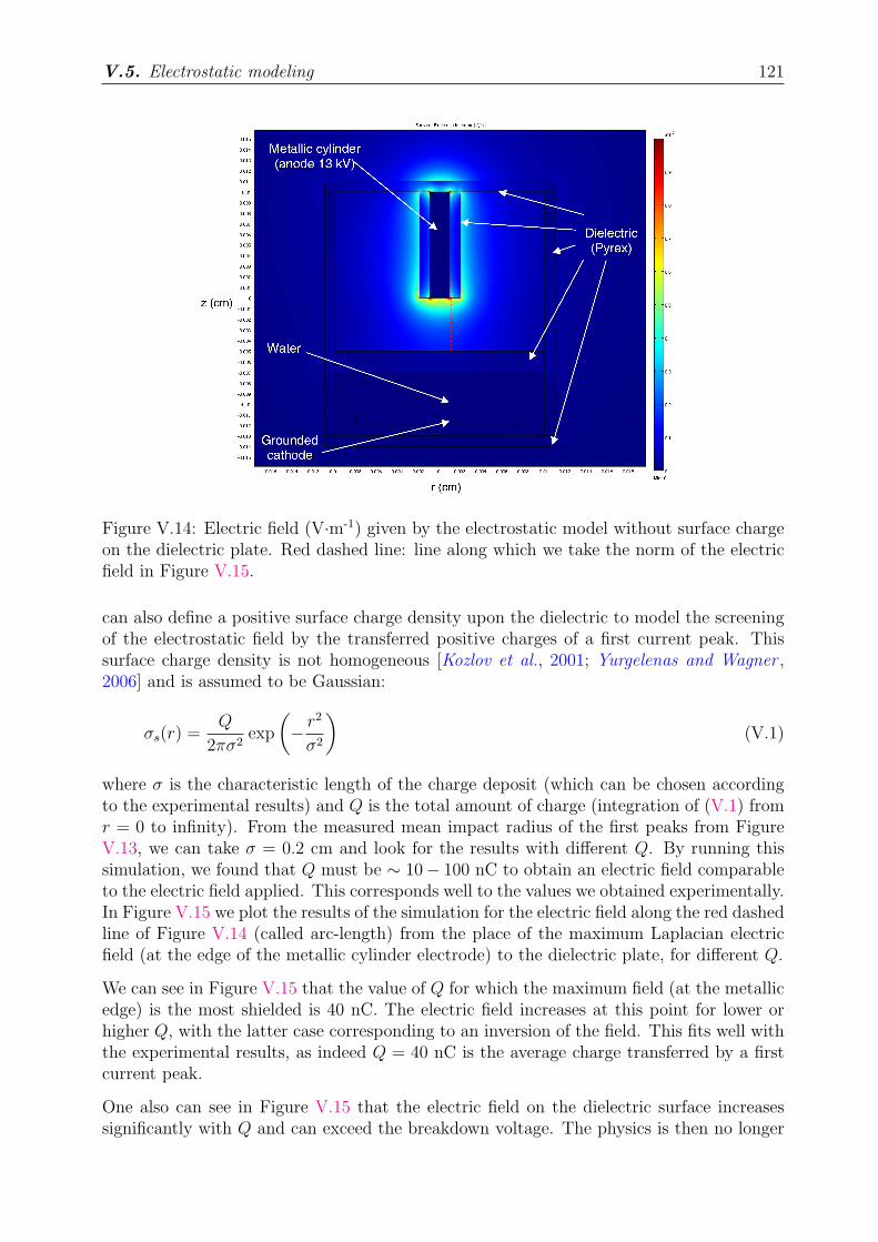
V.5. Electrostatic modeling 121
Figure V.14: Electric field (V·m-1) given by the electrostatic model without surface chargeon the dielectric plate. Red dashed line: line along which we take the norm of the electricfield in Figure V.15.
can also define a positive surface charge density upon the dielectric to model the screeningof the electrostatic field by the transferred positive charges of a first current peak. Thissurface charge density is not homogeneous [Kozlov et al., 2001; Yurgelenas and Wagner ,2006] and is assumed to be Gaussian:
σs(r) =Q
2πσ2exp
(
− r2
σ2
)
(V.1)
where σ is the characteristic length of the charge deposit (which can be chosen accordingto the experimental results) and Q is the total amount of charge (integration of (V.1) fromr = 0 to infinity). From the measured mean impact radius of the first peaks from FigureV.13, we can take σ = 0.2 cm and look for the results with different Q. By running thissimulation, we found that Q must be ∼ 10− 100 nC to obtain an electric field comparableto the electric field applied. This corresponds well to the values we obtained experimentally.In Figure V.15 we plot the results of the simulation for the electric field along the red dashedline of Figure V.14 (called arc-length) from the place of the maximum Laplacian electricfield (at the edge of the metallic cylinder electrode) to the dielectric plate, for different Q.
We can see in Figure V.15 that the value of Q for which the maximum field (at the metallicedge) is the most shielded is 40 nC. The electric field increases at this point for lower orhigher Q, with the latter case corresponding to an inversion of the field. This fits well withthe experimental results, as indeed Q = 40 nC is the average charge transferred by a firstcurrent peak.
One also can see in Figure V.15 that the electric field on the dielectric surface increasessignificantly with Q and can exceed the breakdown voltage. The physics is then no longer
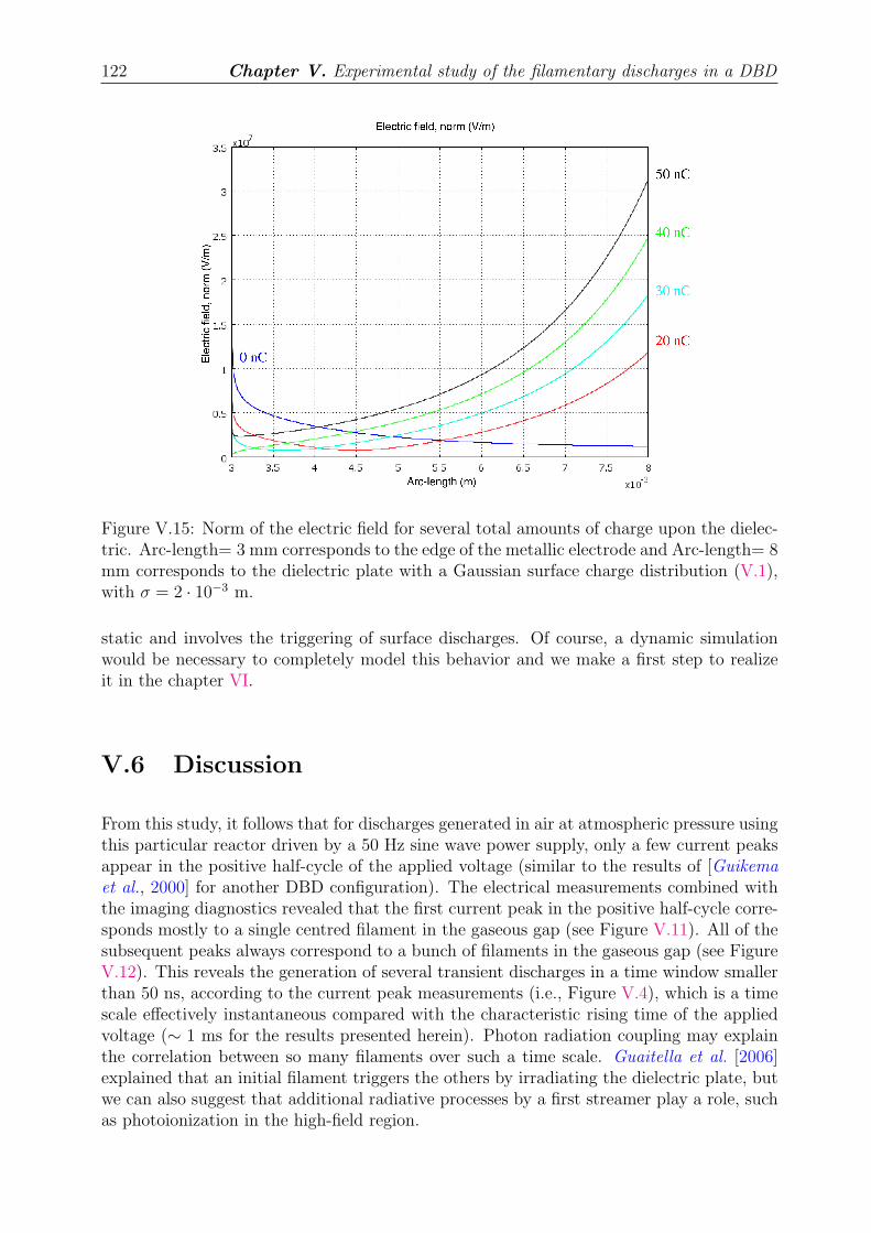
122 Chapter V. Experimental study of the filamentary discharges in a DBD
Figure V.15: Norm of the electric field for several total amounts of charge upon the dielec-tric. Arc-length= 3 mm corresponds to the edge of the metallic electrode and Arc-length= 8mm corresponds to the dielectric plate with a Gaussian surface charge distribution (V.1),with σ = 2 · 10−3 m.
static and involves the triggering of surface discharges. Of course, a dynamic simulationwould be necessary to completely model this behavior and we make a first step to realizeit in the chapter VI.
V.6 Discussion
From this study, it follows that for discharges generated in air at atmospheric pressure usingthis particular reactor driven by a 50 Hz sine wave power supply, only a few current peaksappear in the positive half-cycle of the applied voltage (similar to the results of [Guikemaet al., 2000] for another DBD configuration). The electrical measurements combined withthe imaging diagnostics revealed that the first current peak in the positive half-cycle corre-sponds mostly to a single centred filament in the gaseous gap (see Figure V.11). All of thesubsequent peaks always correspond to a bunch of filaments in the gaseous gap (see FigureV.12). This reveals the generation of several transient discharges in a time window smallerthan 50 ns, according to the current peak measurements (i.e., Figure V.4), which is a timescale effectively instantaneous compared with the characteristic rising time of the appliedvoltage (∼ 1 ms for the results presented herein). Photon radiation coupling may explainthe correlation between so many filaments over such a time scale. Guaitella et al. [2006]explained that an initial filament triggers the others by irradiating the dielectric plate, butwe can also suggest that additional radiative processes by a first streamer play a role, suchas photoionization in the high-field region.
V.6. Discussion 123
Furthermore, we see in Figure V.12 that the subsequent discharges following a first peakdo not reach the center of the dielectric anymore. More precisely, the mean impact radiuswas measured as an increasing function of Vpeak (see Figure V.13). This effect on the layoutof the plasma filaments is due to the charges deposited on the dielectric. It must be notedthat the behavior of the transient filaments and the measurements of the charge transferredby a first current peak are in good agreement with a simple electrostatic model discussed inSection V.5. This model also confirms that the screening mechanism of a DBD, namely thedeposition of charges on a dielectric, changes the entire field configuration in the gaseousgap as well as the propagation of subsequent streamers. As stated in [Kogelschatz , 2002], ina typical discharge situation there is a competition between individual microdischarges forthe available surface area. In the situation we encountered in this chapter, this competitionis dominated by the residual charges already deposited on the dielectric by the previousdischarges, and this effect makes the filaments of successive current peaks extend fartherand farther from the center of the dielectric to deposit their charge. It has to be noted thatin this study we did not observe a single sequence of current peaks in the same positivehalf-cycle of the applied voltage. It was impossible because the readout time of the CCDwas too long.
Moreover, Figure V.9 shows that, for the first peak in the positive half-cycle, the maxi-mum current increases with Vpeak, the applied voltage at which the current peak appears.Therefore, because the charge transferred is related to the screened field, in this experi-mental configuration, the discharge does not occur for a constant voltage in the gaseousgap (meaning the gap above the deposits of charge). Equivalently, the discharge does notoccur at a constant field, presumably the breakdown field, in the high-field region near themetal cylinder edge. Indeed, if the microdischarge occurred at a constant voltage in thegaseous gap (presumably the breakdown voltage in the considered geometry), it would gen-erate always the same current necessary to transfer sufficient charge to screen the electricfield. We propose that the ignition time of the first current peak (of which current-voltagerelationship is shown in Figure V.9) corresponds to the efficiency and the stochasticity ofthe initiation of the ‘pre-breakdown phase’ described in [Kozlov et al., 2001; Yurgelenas andWagner , 2006] or the ‘Townsend phase’ described in [Braun et al., 1992]. In the config-uration used in this chapter, the pre-breakdown phase activity occurs at the edge of themetallic cylinder electrode, where the radius of curvature is smallest and hence where theelectric field is strongest. The moment of the beginning of the Townsend phase is suspectedhere to be influenced by the charge deposited on the dielectric, as surface charge can af-fect the secondary emission from the dielectric. The current of this microdischarge is thendetermined by the electric field at the metallic electrode when the microdischarge finallyoccurs.
The impact of the amount of charge deposited on the dielectric plate on (1) the multi-filament behavior and (2) the intensity of the discharges cannot be resolved solely by usinga static model; a dynamic model of streamer propagation toward a charged dielectric plateis required.
124 Chapter V. Experimental study of the filamentary discharges in a DBD
V.7 Conclusions
The electrical measurements combined with the imaging diagnostics revealed that the firstcurrent peak in the positive half-cycle corresponds mostly to a single centred filament inthe gaseous gap, but all of the subsequent peaks always correspond to organized multi-filamentary discharges in the gaseous gap. Both kinds of discharges are strongly branchingover the dielectric material.
The spatial organization of plasma filaments is strongly affected by the deposited chargeson the dielectric material. A first discharge in the positive half-cycle deposits charges closeto the center of the dielectric plate. Subsequent discharges are affected by these surfacecharges and plasma filaments then impact the dielectric farther and farther from the centerof the dielectric plate.
The first current peak ignition time corresponds to the efficiency and the stochasticity of theinitiation of the ‘pre-breakdown phase’ and consequently the amount of transferred chargesin the positive half-cycle is correlated with the voltage at the metallic electrode when a firstcurrent peak occurs. This has an impact on the temporal organization of discharges in onepositive half-cycle.
A model of the streamers dynamics in such an experimental configuration is required tobetter understand the impact of a dielectric material, and the charges deposited upon it,on the streamers dynamics. Such a study is presented in Chapter VI.
Chapter VI
Simulation of streamer propagation ina point-to-plane DBD configuration
Table of ContentsVI.1 Introduction . . . . . . . . . . . . . . . . . . . . . . . . . . . . . . 126
VI.2 Discretization of a Poisson’s equation with variable coefficients 128
VI.3 Analytical electrostatic study of the point-to-plane configura-tion with dielectric . . . . . . . . . . . . . . . . . . . . . . . . . . 129
VI.3.1 Electric potential . . . . . . . . . . . . . . . . . . . . . . . . . . . 130
VI.3.2 Electric field . . . . . . . . . . . . . . . . . . . . . . . . . . . . . 131
VI.3.3 Approximation of the analytical model . . . . . . . . . . . . . . . 131
VI.4 Simulation of streamer dynamics . . . . . . . . . . . . . . . . . . 132
VI.4.1 Streamer propagation in the gas gap . . . . . . . . . . . . . . . . 134
VI.4.2 Interaction between the streamer and the dielectric . . . . . . . . 138
VI.4.3 Perfectly emitting dielectric surface and electron density in thevicinity of the anode tip . . . . . . . . . . . . . . . . . . . . . . . 141
VI.5 Conclusions . . . . . . . . . . . . . . . . . . . . . . . . . . . . . . . 143
126 Chapter VI. Simulation of a point-to-plane DBD
VI.1 Introduction
As stated in Chapter V, in order to further advance in the understanding of the dis-charge, it is necessary to study streamer dynamics in Dielectric Barrier Discharges.
However, the experimental setup used in this Chapter has a complex geometry, especiallywith a dielectric around the tip anode. Therefore, three-dimensional computations wouldbe necessary to simulate this discharge.
In this chapter, we consider a simplified axisymmetric configuration using a hyperboloidpoint-to-plane geometry with a dielectric material on the plane cathode. We study thestreamer dynamics in this configuration, and we show that the results obtained are in goodagreement with the experimental results obtained in Chapter V.
The point-to-plane configuration studied is depicted in Figure VI.1 and is similar to the onepresented in Chapter IV, with the addition of a dielectric material on the plane cathode.The configuration is axisymmetric, with a needle anode that is assumed to be an infinitehyperboloid body of revolution about the axis of symmetry. The cathode is the planeperpendicular to the axis of symmetry and coinciding with the origin of x coordinate.
Near the needle electrode, the electric potential is calculated by solving the discretized Pois-son’s equation (II.2) using the Ghost Fluid Method (see Chapter IV). As for the case withno dielectric material, the analytical Dirichlet boundary condition is used in order to reducethe time consumption of the simulation. Indeed, as stated at the end of Section IV.2.1,solving Poisson’s equation accurately using the homogeneous Neumann boundary condition(~∇V · ~n = 0, where ~n is the unit vector normal to the surface boundary) would be moretime-consuming as it requires expanding the computational domain and thus significantlyincreasing the computation time of the simulation.
In Figure VI.1, we have divided the electrode gap into two domains Ω1 and Ω2. Thedomain Ω1 is constituted of air at t = 0, therefore the dielectric permittivity in this domainis ǫ = ǫ0; this is the domain in which the discharges propagate. The domain Ω2 is thedielectric material with permittivity ǫ = ǫ2.
To take into account several domains with different dielectric permittivities, the governingequation for the electric field is:
~∇ · ~D = ρ (VI.1)
where ~D = ǫ0~E + ~P is the electric displacement field, and ~P the polarization density of
the material. For linear and isotropic media, ~D = ǫ ~E ≡ ǫrǫ0~E, where ǫ and ǫr are scalars.
Thus, as ~E = −~∇V , the equation governing the electric potential is Poisson’s equation
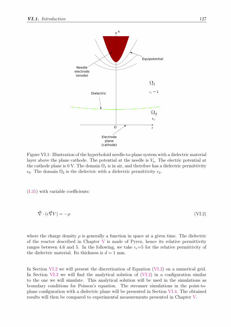
VI.1. Introduction 127
Figure VI.1: Illustration of the hyperboloid needle-to-plane system with a dielectric materiallayer above the plane cathode. The potential at the needle is Va. The electric potential atthe cathode plane is 0 V. The domain Ω1 is in air, and therefore has a dielectric permittivityǫ0. The domain Ω2 is the dielectric with a dielectric permittivity ǫ2.
(I.31) with variable coefficients:
~∇ · (ǫ~∇V ) = −ρ (VI.2)
where the charge density ρ is generally a function in space at a given time. The dielectricof the reactor described in Chapter V is made of Pyrex, hence its relative permittivityranges between 4.6 and 5. In the following, we take ǫr=5 for the relative permittivity ofthe dielectric material. Its thickness is d = 1 mm.
In Section VI.2 we will present the discretization of Equation (VI.2) on a numerical grid.In Section VI.3 we will find the analytical solution of (VI.2) in a configuration similarto the one we will simulate. This analytical solution will be used in the simulations asboundary conditions for Poisson’s equation. The streamer simulations in the point-to-plane configuration with a dielectric plane will be presented in Section VI.4. The obtainedresults will then be compared to experimental measurements presented in Chapter V.
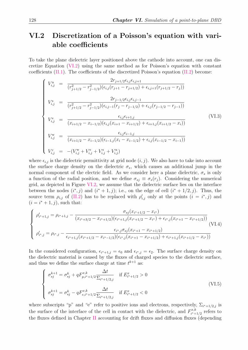
128 Chapter VI. Simulation of a point-to-plane DBD
VI.2 Discretization of a Poisson’s equation with vari-able coefficients
To take the plane dielectric layer positioned above the cathode into account, one can dis-cretize Equation (VI.2) using the same method as for Poisson’s equation with constantcoefficients (II.1). The coefficients of the discretized Poisson’s equation (II.2) become:
V ni,j =
2rj+1/2ǫi,jǫi,j+1
(r2j+1/2 − r2
j−1/2)(ǫi,j(rj+1 − rj+1/2) + ǫi,j+1(rj+1/2 − rj))
V si,j =
2rj−1/2ǫi,jǫi,j−1
(r2j+1/2 − r2
j−1/2)(ǫi,j−1(rj − rj−1/2) + ǫi,j(rj−1/2 − rj−1))
V ei,j =
ǫi,jǫi+1,j
(xi+1/2 − xi−1/2)(ǫi,j(xi+1 − xi+1/2) + ǫi+1,j(xi+1/2 − xi))
V wi,j =
ǫi,jǫi−1,j
(xi+1/2 − xi−1/2)(ǫi−1,j(xi − xi−1/2) + ǫi,j(xi−1/2 − xi−1))
V ci,j = −(V w
i,j + V ei,j + V s
i,j + V ni,j)
(VI.3)
where ǫi,j is the dielectric permittivity at grid node (i, j). We also have to take into accountthe surface charge density on the dielectric σs, which causes an additional jump in thenormal component of the electric field. As we consider here a plane dielectric, σs is onlya function of the radial position, and we define σsj ≡ σs(rj). Considering the numericalgrid, as depicted in Figure VI.2, we assume that the dielectric surface lies on the interfacebetween the nodes (i∗, j) and (i∗ + 1, j); i.e., on the edge of cell (i∗ + 1/2, j). Thus, thesource term ρi,j of (II.2) has to be replaced with ρ′
i,j only at the points (i = i∗, j) and(i = i∗ + 1, j), such that:
ρ′i∗+1,j = ρi∗+1,j −
σsj(xi∗+1/2 − xi∗)
(xi∗+3/2 − xi∗+1/2)(ǫi∗+1,j(xi∗+1/2 − xi∗) + ǫi∗,j(xi∗+1 − xi∗+1/2))
ρ′i∗,j = ρi∗,j −
ǫi∗,jσsj(xi∗+1 − xi∗+1/2)
ǫi∗+1,j(xi∗+1/2 − xi∗−1/2)(ǫi∗,j(xi∗+1 − xi∗+1/2) + ǫi∗+1,j(xi∗+1/2 − xi∗))
(VI.4)
In the considered configuration, ǫi∗+1,j = ǫ0 and ǫi∗,j = ǫ2. The surface charge density onthe dielectric material is caused by the fluxes of charged species to the dielectric surface,and thus we define the surface charge at time tk+1 as:
σk+1sj = σk
sj + qF x,kp,i∗+1/2
∆t
Σi∗+1/2,j
if Exi∗+1/2 > 0
σk+1sj = σk
sj − qF x,ke,i∗+1/2
∆t
Σi∗+1/2,j
if Exi∗+1/2 < 0
(VI.5)
where subscripts “p” and “e” refer to positive ions and electrons, respectively, Σi∗+1/2,j isthe surface of the interface of the cell in contact with the dielectric, and F x,k
i∗+1/2 refers tothe fluxes defined in Chapter II accounting for drift fluxes and diffusion fluxes (depending
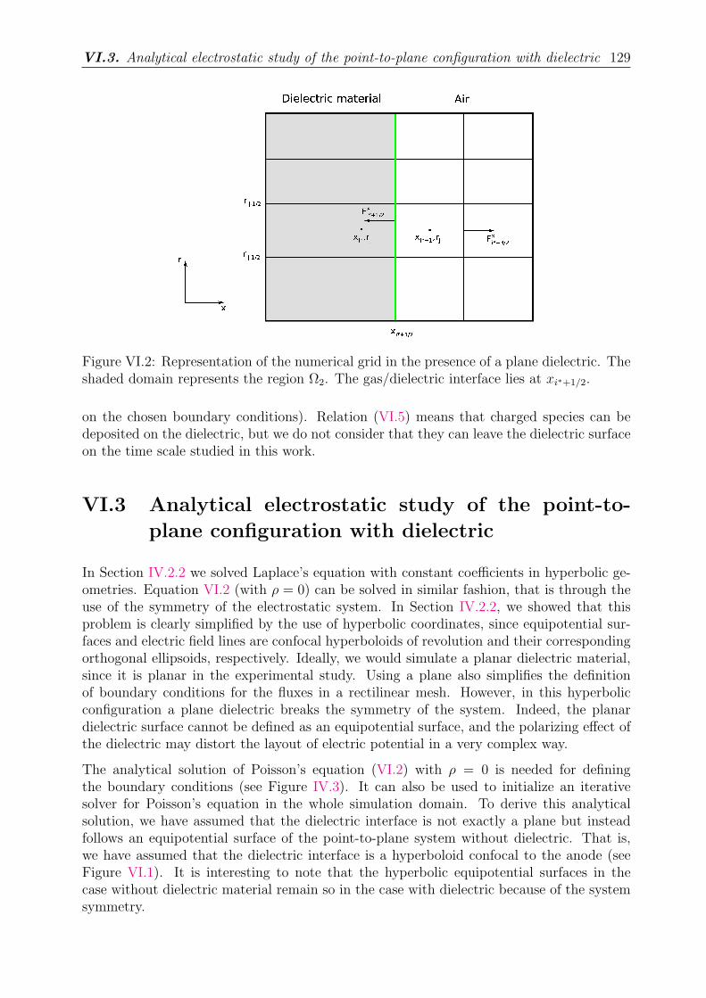
VI.3. Analytical electrostatic study of the point-to-plane configuration with dielectric 129
Figure VI.2: Representation of the numerical grid in the presence of a plane dielectric. Theshaded domain represents the region Ω2. The gas/dielectric interface lies at xi∗+1/2.
on the chosen boundary conditions). Relation (VI.5) means that charged species can bedeposited on the dielectric, but we do not consider that they can leave the dielectric surfaceon the time scale studied in this work.
VI.3 Analytical electrostatic study of the point-to-plane configuration with dielectric
In Section IV.2.2 we solved Laplace’s equation with constant coefficients in hyperbolic ge-ometries. Equation VI.2 (with ρ = 0) can be solved in similar fashion, that is through theuse of the symmetry of the electrostatic system. In Section IV.2.2, we showed that thisproblem is clearly simplified by the use of hyperbolic coordinates, since equipotential sur-faces and electric field lines are confocal hyperboloids of revolution and their correspondingorthogonal ellipsoids, respectively. Ideally, we would simulate a planar dielectric material,since it is planar in the experimental study. Using a plane also simplifies the definitionof boundary conditions for the fluxes in a rectilinear mesh. However, in this hyperbolicconfiguration a plane dielectric breaks the symmetry of the system. Indeed, the planardielectric surface cannot be defined as an equipotential surface, and the polarizing effect ofthe dielectric may distort the layout of electric potential in a very complex way.
The analytical solution of Poisson’s equation (VI.2) with ρ = 0 is needed for definingthe boundary conditions (see Figure IV.3). It can also be used to initialize an iterativesolver for Poisson’s equation in the whole simulation domain. To derive this analyticalsolution, we have assumed that the dielectric interface is not exactly a plane but insteadfollows an equipotential surface of the point-to-plane system without dielectric. That is,we have assumed that the dielectric interface is a hyperboloid confocal to the anode (seeFigure VI.1). It is interesting to note that the hyperbolic equipotential surfaces in thecase without dielectric material remain so in the case with dielectric because of the systemsymmetry.
130 Chapter VI. Simulation of a point-to-plane DBD
We recall the transformation from Cartesian to hyperbolic coordinates (IV.7):
x = αξ(1 + η2)1/2
r = αη(1 − ξ2)1/2 (VI.6)
where ξ2 < 1 and α 6= 0. The equipotential surfaces of the problem are defined by ξ(x, r) =C, where C is a constant. We note that ξ = ξ0 defines the anode surface, ξ = 0 defines thecathode plane, and ξ = ξ1 defines the dielectric interface.
To define the dielectric interface, we consider a hyperboloid equipotential surface ξ = ξ1
close enough to the cathode to be considered a good approximation of a plane dielectric.
VI.3.1 Electric potential
The relative dielectric permittivity ǫr is a constant in each domain Ω1 and Ω2. Thus it ispossible to solve for the electric potential in each domain separately. Given the symmetriesof the system, the solution in each domain follows from the electric potential given inSection IV.2.2 (i.e., Equation (IV.9)):
V1 =A
2log
1 + ξ
1 − ξ+ B in Ω1
V2 =A′
2log
1 + ξ
1 − ξ+ B′ in Ω2
(VI.7)
where A, B, A′, and B′ are the four unknowns determined according to the four boundarycondition equations:
V1(ξ0) =A
2log
1 + ξ0
1 − ξ0
+ B = Va (VI.8)
V2(ξ = 0) = B′ = 0 (VI.9)
V1(ξ1) = V2(ξ1) (VI.10)
ǫ0(~n · ~E|ξ>ξ1,ξ→ξ1) − ǫ2(~n · ~E|ξ<ξ1,ξ→ξ1) = σs = 0 (VI.11)
where ~n is the unit vector normal to the dielectric interface, and σs is the surface chargedensity upon the dielectric material, which is considered to be zero in this analytical study.Equation (VI.8) defines the potential value Va at the anode. Equation (VI.9) sets the zero-potential value at the cathode. Equation (VI.10) is the condition for the electric potentialcontinuity across the dielectric interface. Finally, Equation (VI.11) defines the discontinuityof the normal component of the electric field through the dielectric interface [e.g., Durand ,1966a, c].
From the formulation of gradient in this coordinates system (IV.12), one has:
~E = −~∇V = − 1
Ξ
∂V
∂ξ~uη (VI.12)
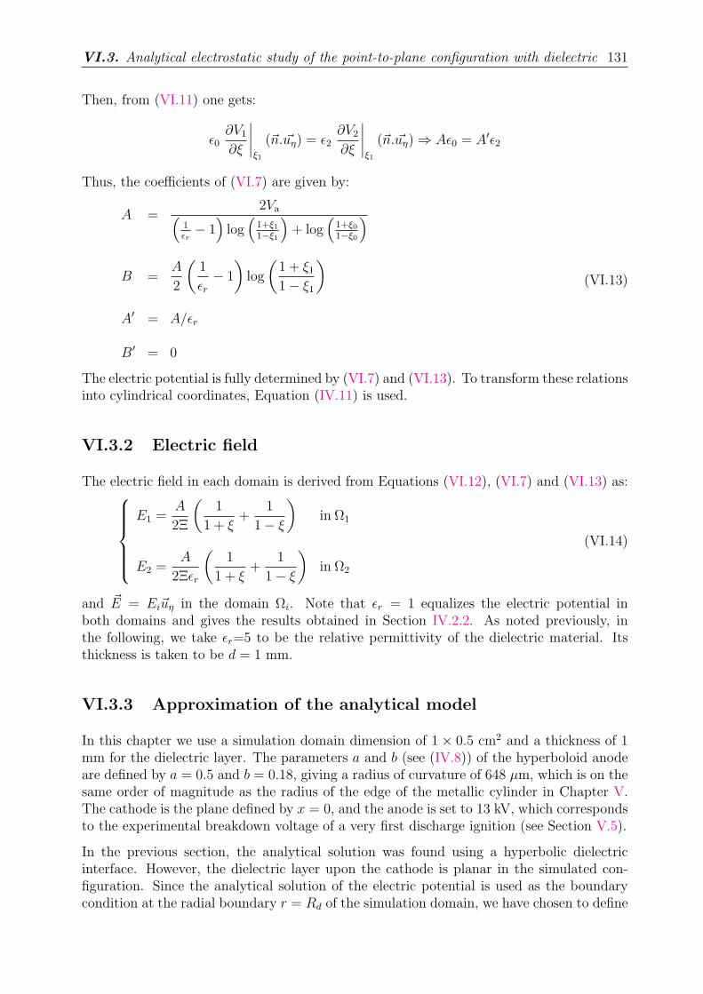
VI.3. Analytical electrostatic study of the point-to-plane configuration with dielectric 131
Then, from (VI.11) one gets:
ǫ0∂V1
∂ξ
∣
∣
∣
∣
ξ1
(~n. ~uη) = ǫ2∂V2
∂ξ
∣
∣
∣
∣
ξ1
(~n. ~uη) ⇒ Aǫ0 = A′ǫ2
Thus, the coefficients of (VI.7) are given by:
A =2Va
(
1ǫr− 1)
log(
1+ξ11−ξ1
)
+ log(
1+ξ01−ξ0
)
B =A
2
(
1
ǫr
− 1
)
log
(
1 + ξ1
1 − ξ1
)
A′ = A/ǫr
B′ = 0
(VI.13)
The electric potential is fully determined by (VI.7) and (VI.13). To transform these relationsinto cylindrical coordinates, Equation (IV.11) is used.
VI.3.2 Electric field
The electric field in each domain is derived from Equations (VI.12), (VI.7) and (VI.13) as:
E1 =A
2Ξ
(
1
1 + ξ+
1
1 − ξ
)
in Ω1
E2 =A
2Ξǫr
(
1
1 + ξ+
1
1 − ξ
)
in Ω2
(VI.14)
and ~E = Ei~uη in the domain Ωi. Note that ǫr = 1 equalizes the electric potential inboth domains and gives the results obtained in Section IV.2.2. As noted previously, inthe following, we take ǫr=5 to be the relative permittivity of the dielectric material. Itsthickness is taken to be d = 1 mm.
VI.3.3 Approximation of the analytical model
In this chapter we use a simulation domain dimension of 1 × 0.5 cm2 and a thickness of 1mm for the dielectric layer. The parameters a and b (see (IV.8)) of the hyperboloid anodeare defined by a = 0.5 and b = 0.18, giving a radius of curvature of 648 µm, which is on thesame order of magnitude as the radius of the edge of the metallic cylinder in Chapter V.The cathode is the plane defined by x = 0, and the anode is set to 13 kV, which correspondsto the experimental breakdown voltage of a very first discharge ignition (see Section V.5).
In the previous section, the analytical solution was found using a hyperbolic dielectricinterface. However, the dielectric layer upon the cathode is planar in the simulated con-figuration. Since the analytical solution of the electric potential is used as the boundarycondition at the radial boundary r = Rd of the simulation domain, we have chosen to define
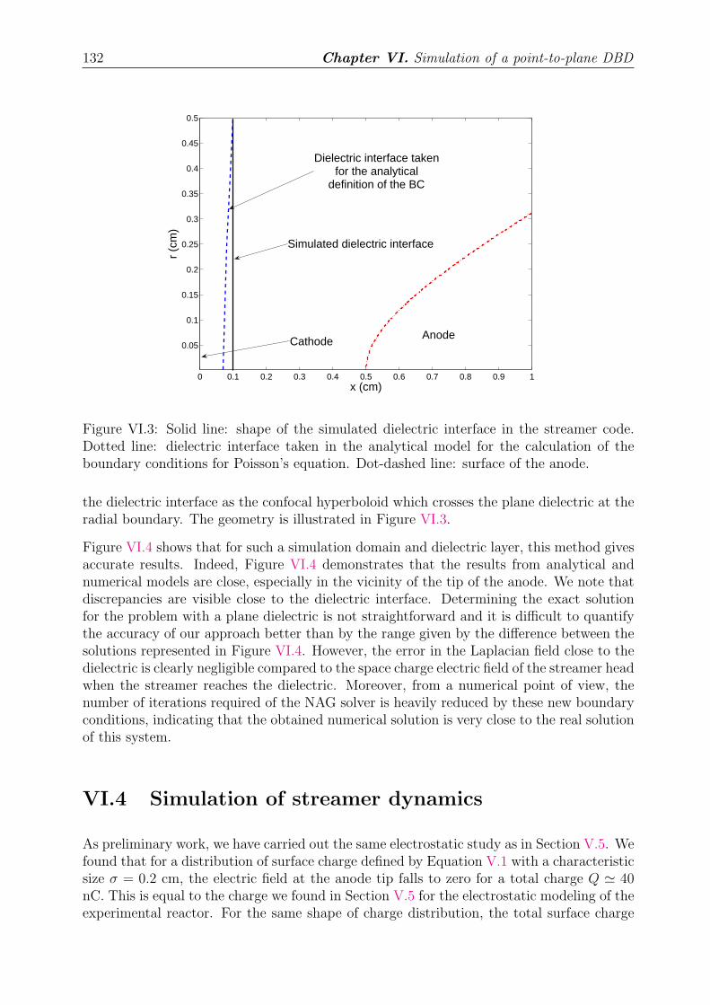
132 Chapter VI. Simulation of a point-to-plane DBD
x (cm)
r (c
m)
0 0.1 0.2 0.3 0.4 0.5 0.6 0.7 0.8 0.9 1
0.05
0.1
0.15
0.2
0.25
0.3
0.35
0.4
0.45
0.5
Simulated dielectric interface
Dielectric interface taken for the analytical
definition of the BC
AnodeCathode
Figure VI.3: Solid line: shape of the simulated dielectric interface in the streamer code.Dotted line: dielectric interface taken in the analytical model for the calculation of theboundary conditions for Poisson’s equation. Dot-dashed line: surface of the anode.
the dielectric interface as the confocal hyperboloid which crosses the plane dielectric at theradial boundary. The geometry is illustrated in Figure VI.3.
Figure VI.4 shows that for such a simulation domain and dielectric layer, this method givesaccurate results. Indeed, Figure VI.4 demonstrates that the results from analytical andnumerical models are close, especially in the vicinity of the tip of the anode. We note thatdiscrepancies are visible close to the dielectric interface. Determining the exact solutionfor the problem with a plane dielectric is not straightforward and it is difficult to quantifythe accuracy of our approach better than by the range given by the difference between thesolutions represented in Figure VI.4. However, the error in the Laplacian field close to thedielectric is clearly negligible compared to the space charge electric field of the streamer headwhen the streamer reaches the dielectric. Moreover, from a numerical point of view, thenumber of iterations required of the NAG solver is heavily reduced by these new boundaryconditions, indicating that the obtained numerical solution is very close to the real solutionof this system.
VI.4 Simulation of streamer dynamics
As preliminary work, we have carried out the same electrostatic study as in Section V.5. Wefound that for a distribution of surface charge defined by Equation V.1 with a characteristicsize σ = 0.2 cm, the electric field at the anode tip falls to zero for a total charge Q ≃ 40nC. This is equal to the charge we found in Section V.5 for the electrostatic modeling of theexperimental reactor. For the same shape of charge distribution, the total surface charge
VI.4. Simulation of streamer dynamics 133
0 0.05 0.1 0.15 0.2 0.25 0.3 0.35 0.4 0.45 0.50
2
4
6
8
10
12
14x 10
4
x (cm)
Ele
ctric
fiel
d (V
/cm
)
Figure VI.4: Magnitude of the electric field along the axis of symmetry, calculated for settingthe Dirichlet boundary conditions. Solid line: numerical solution of Laplace’s equationcomputed on a 1000× 500 Cartesian grid. Dashed line: analytical solution used for settingthe Dirichlet boundary condition.
Q ≃ 35 nC is required to decrease the electric field to the breakdown field Ek ≃ 30 kV/cm.Considering Section V.5, this indicates that the simplified configuration considered in thischapter can be used to obtain the order of magnitude for the main electrical characteristicsrelated to a first current peak in the positive half-cycle of the experimental work discussedin Chapter V.
In the following, we study streamer dynamics in the above defined configuration. As forthe point-to-plane configuration without dielectric studied in Section IV.3.2, we initiate thepositive streamer by placing a Gaussian spot of neutral plasma close to the anode tip:
np(x, r)|t=0 = ne(x, r)|t=0 = n0 exp
[
− r2
σ2r
− (x − x0)2
σ2x
]
(VI.15)
where x0 = 0.5−σx, σx = 0.01 cm, and σr = 0.01 cm. At t = 0, there are no negative ions.The initial maximum density is n0 = 1014 cm-3.
In this study we have used the same transport parameters and reaction rates as in [Ku-likovsky , 1998], and we have used the positive ion mobility from [Morrow and Lowke, 1997].Given the complexity of the simulated problem, the results shown in the present work arecomputed using the upwind scheme. We mentioned in Chapter II that the upwind schemeis able to provide essential information on streamer dynamics, although it overestimatesthe electron density and the electric field.
The simulation domain is 1×0.5 cm2, discretized on a 1597×344 grid. In the axial direction,the grid is:
• uniform with a cell size of ∆x = 5 µm from x = 0 to 0.75 cm
134 Chapter VI. Simulation of a point-to-plane DBD
• refined around the dielectric interface with ∆x = 1 µm from x = 0.75 cm to 0.125 cm
• non-uniform from x = 0.125 cm to 0.15 cm with a geometric expansion ∆xi =1.1∆xi−1 up to ∆x = 5 µm at x = 0.15 cm
• uniform with ∆x = 5 µm until x = 0.55 cm
• non-uniform, following a geometric progression with a ratio of 1.1 up to x = 1 cm
In the radial direction we have used a grid that is:
• uniform with ∆r = 5 µm up to r = 0.15 cm
• non-uniform, following a geometric progression with a ratio of 1.1 up to r = 0.5 cm
The photoionization source term has been computed using the three-group SP3 approachwith Larsen’s boundary conditions (see Chapter III).
The boundary conditions for fluxes at the dielectric surface have been observed to play asignificant role after the streamer contacts the dielectric material. In the following, theboundary conditions are zero for the diffusion and drift fluxes. We model the secondaryemission due to ion bombardment by the second Townsend coefficient γ defined as theaverage number of electrons produced by one ion as it impacts the dielectric material. Atthe end of this chapter we also show some results obtained with the dielectric acting as aperfectly emitting boundary, that is with a zero-gradient condition on the electron density∂ne
∂x
∣
∣
x=0.1= 0.
VI.4.1 Streamer propagation in the gas gap
At the beginning of the simulation, the positive streamer is initiated close to the anode tipand then propagates towards the grounded plane. As an example of the results obtained,Figures VI.5 and VI.6 show cross-sectional views of the electron density and the magnitudeof the electric field, respectively, at t = 3 ns.
We found that the secondary emission via ion bombardment at the dielectric interface doesnot play any role during streamer propagation in the gas gap. Conversely, the role ofsecondary emission becomes significant when the streamer reaches the dielectric surface.This will be discussed in the next section.
The propagation of the streamer from the anode to the dielectric surface lasts ∼4.5 ns.During this phase, the ions and electrons near the dielectric surface are produced only bythe photoionization. Figure VI.7 shows that the increase of the surface charge density dueto the ion drift towards the dielectric is slow. During the streamer propagation, the surfacecharge density does not increase sufficiently to distort the Laplacian electric field. FigureVI.7 also illustrates the modification of the surface charge variation at t = 4.5 ns, indicatingthe interaction of the streamer with the dielectric surface.
To compare our results with experiments, we have also calculated the electric current col-lected by the cathode. The cathode plane is under the dielectric material and therefore thecollected current at the cathode is the displacement current:
I =
∫
S
∂ ~D
∂t· d~S = ǫ2
∫
S
∂ ~E
∂t· d~S (VI.16)
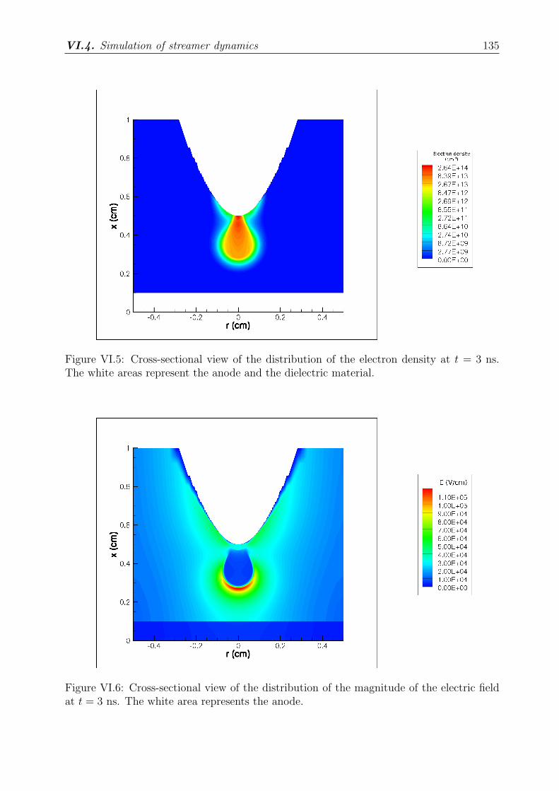
VI.4. Simulation of streamer dynamics 135
Figure VI.5: Cross-sectional view of the distribution of the electron density at t = 3 ns.The white areas represent the anode and the dielectric material.
Figure VI.6: Cross-sectional view of the distribution of the magnitude of the electric fieldat t = 3 ns. The white area represents the anode.
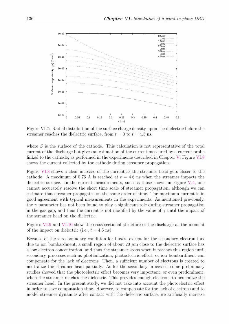
136 Chapter VI. Simulation of a point-to-plane DBD
1e-20
1e-19
1e-18
1e-17
1e-16
1e-15
1e-14
1e-13
0 0.05 0.1 0.15 0.2 0.25 0.3 0.35 0.4 0.45 0.5
Sur
face
cha
rge
dens
ity σ
s(r)
(C
/cm
2 )
r (cm)
0.5 ns1 ns
1.5 ns2 ns
2.5 ns3 ns
3.5 ns4 ns
4.5 ns
Figure VI.7: Radial distribution of the surface charge density upon the dielectric before thestreamer reaches the dielectric surface, from t = 0 to t = 4.5 ns.
where S is the surface of the cathode. This calculation is not representative of the totalcurrent of the discharge but gives an estimation of the current measured by a current probelinked to the cathode, as performed in the experiments described in Chapter V. Figure VI.8shows the current collected by the cathode during streamer propagation.
Figure VI.8 shows a clear increase of the current as the streamer head gets closer to thecathode. A maximum of 0.76 A is reached at t = 4.6 ns when the streamer impacts thedielectric surface. In the current measurements, such as those shown in Figure V.4, onecannot accurately resolve the short time scale of streamer propagation, although we canestimate that streamer propagates on the same order of time. The maximum current is ingood agreement with typical measurements in the experiments. As mentioned previously,the γ parameter has not been found to play a significant role during streamer propagationin the gas gap, and thus the current is not modified by the value of γ until the impact ofthe streamer head on the dielectric.
Figures VI.9 and VI.10 show the cross-sectional structure of the discharge at the momentof the impact on dielectric (i.e., t = 4.5 ns).
Because of the zero boundary condition for fluxes, except for the secondary electron fluxdue to ion bombardment, a small region of about 20 µm close to the dielectric surface hasa low electron concentration, and thus the streamer stops when it reaches this region untilsecondary processes such as photionization, photoelectric effect, or ion bombardment cancompensate for the lack of electrons. Then, a sufficient number of electrons is created toneutralize the streamer head partially. As for the secondary processes, some preliminarystudies showed that the photoelectric effect becomes very important, or even predominant,when the streamer reaches the dielectric. This provides enough electrons to neutralize thestreamer head. In the present study, we did not take into account the photoelectric effectin order to save computation time. However, to compensate for the lack of electrons and tomodel streamer dynamics after contact with the dielectric surface, we artificially increase
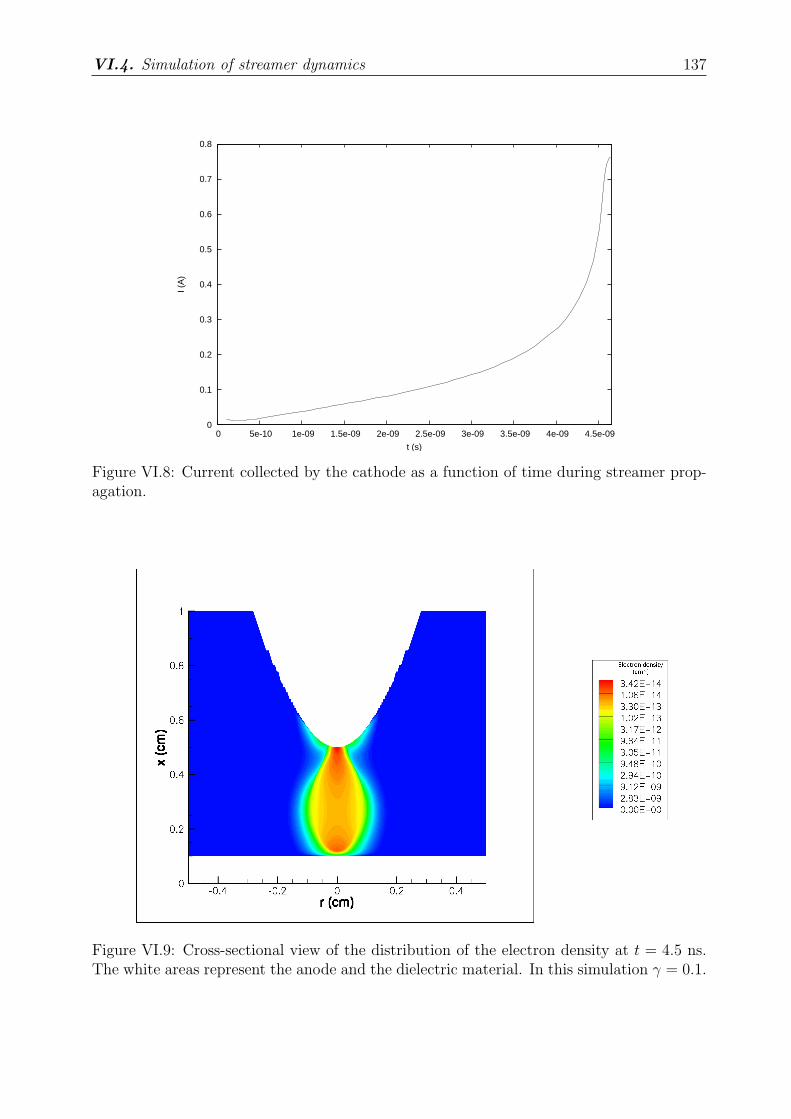
VI.4. Simulation of streamer dynamics 137
0
0.1
0.2
0.3
0.4
0.5
0.6
0.7
0.8
0 5e-10 1e-09 1.5e-09 2e-09 2.5e-09 3e-09 3.5e-09 4e-09 4.5e-09
I (A
)
t (s)
Figure VI.8: Current collected by the cathode as a function of time during streamer prop-agation.
Figure VI.9: Cross-sectional view of the distribution of the electron density at t = 4.5 ns.The white areas represent the anode and the dielectric material. In this simulation γ = 0.1.
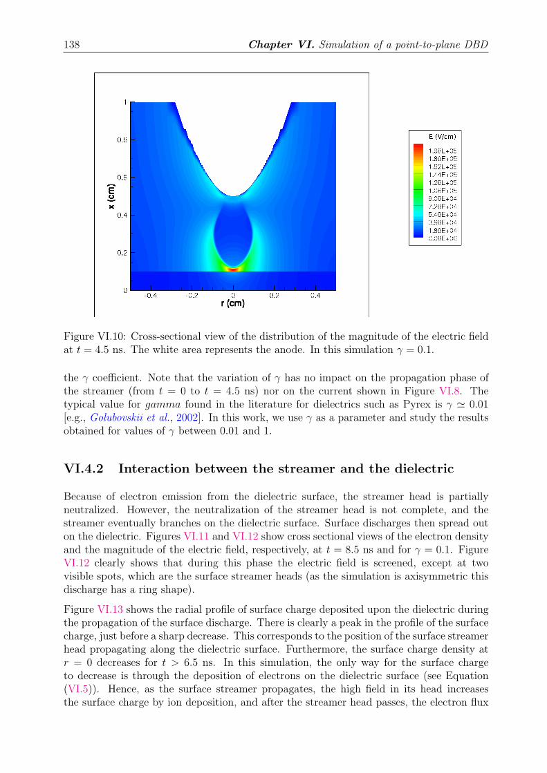
138 Chapter VI. Simulation of a point-to-plane DBD
Figure VI.10: Cross-sectional view of the distribution of the magnitude of the electric fieldat t = 4.5 ns. The white area represents the anode. In this simulation γ = 0.1.
the γ coefficient. Note that the variation of γ has no impact on the propagation phase ofthe streamer (from t = 0 to t = 4.5 ns) nor on the current shown in Figure VI.8. Thetypical value for gamma found in the literature for dielectrics such as Pyrex is γ ≃ 0.01[e.g., Golubovskii et al., 2002]. In this work, we use γ as a parameter and study the resultsobtained for values of γ between 0.01 and 1.
VI.4.2 Interaction between the streamer and the dielectric
Because of electron emission from the dielectric surface, the streamer head is partiallyneutralized. However, the neutralization of the streamer head is not complete, and thestreamer eventually branches on the dielectric surface. Surface discharges then spread outon the dielectric. Figures VI.11 and VI.12 show cross sectional views of the electron densityand the magnitude of the electric field, respectively, at t = 8.5 ns and for γ = 0.1. FigureVI.12 clearly shows that during this phase the electric field is screened, except at twovisible spots, which are the surface streamer heads (as the simulation is axisymmetric thisdischarge has a ring shape).
Figure VI.13 shows the radial profile of surface charge deposited upon the dielectric duringthe propagation of the surface discharge. There is clearly a peak in the profile of the surfacecharge, just before a sharp decrease. This corresponds to the position of the surface streamerhead propagating along the dielectric surface. Furthermore, the surface charge density atr = 0 decreases for t > 6.5 ns. In this simulation, the only way for the surface chargeto decrease is through the deposition of electrons on the dielectric surface (see Equation(VI.5)). Hence, as the surface streamer propagates, the high field in its head increasesthe surface charge by ion deposition, and after the streamer head passes, the electron flux
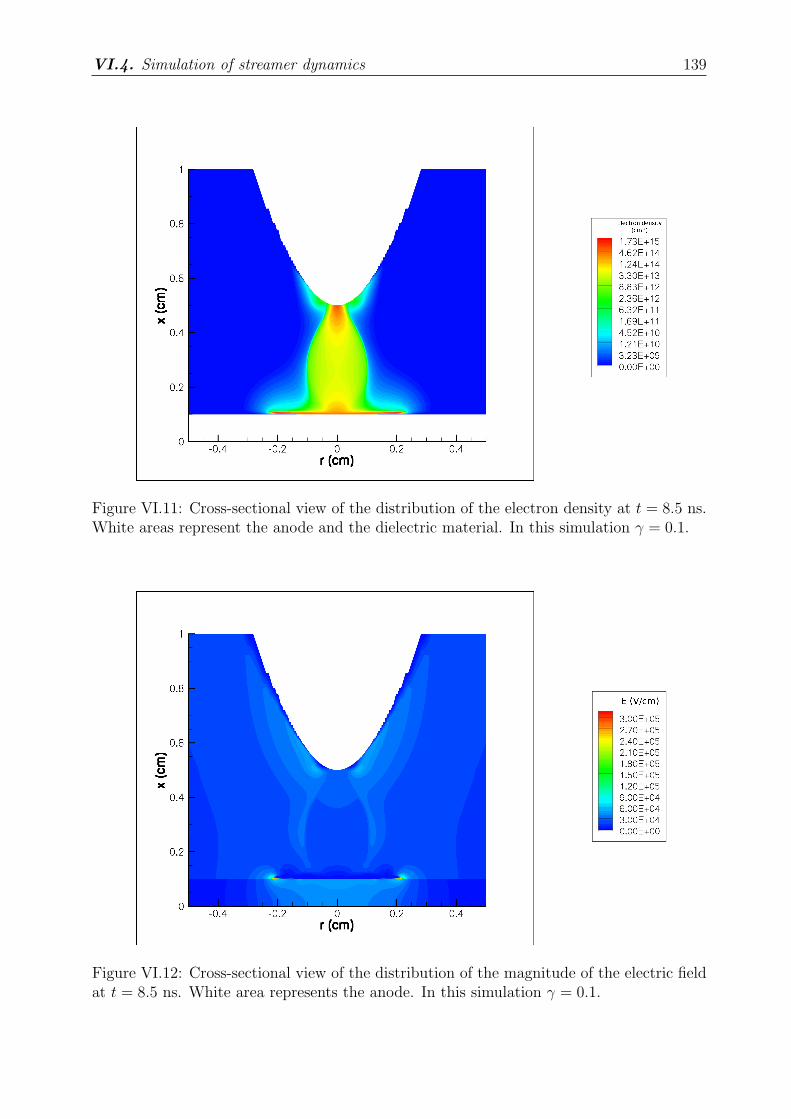
VI.4. Simulation of streamer dynamics 139
Figure VI.11: Cross-sectional view of the distribution of the electron density at t = 8.5 ns.White areas represent the anode and the dielectric material. In this simulation γ = 0.1.
Figure VI.12: Cross-sectional view of the distribution of the magnitude of the electric fieldat t = 8.5 ns. White area represents the anode. In this simulation γ = 0.1.
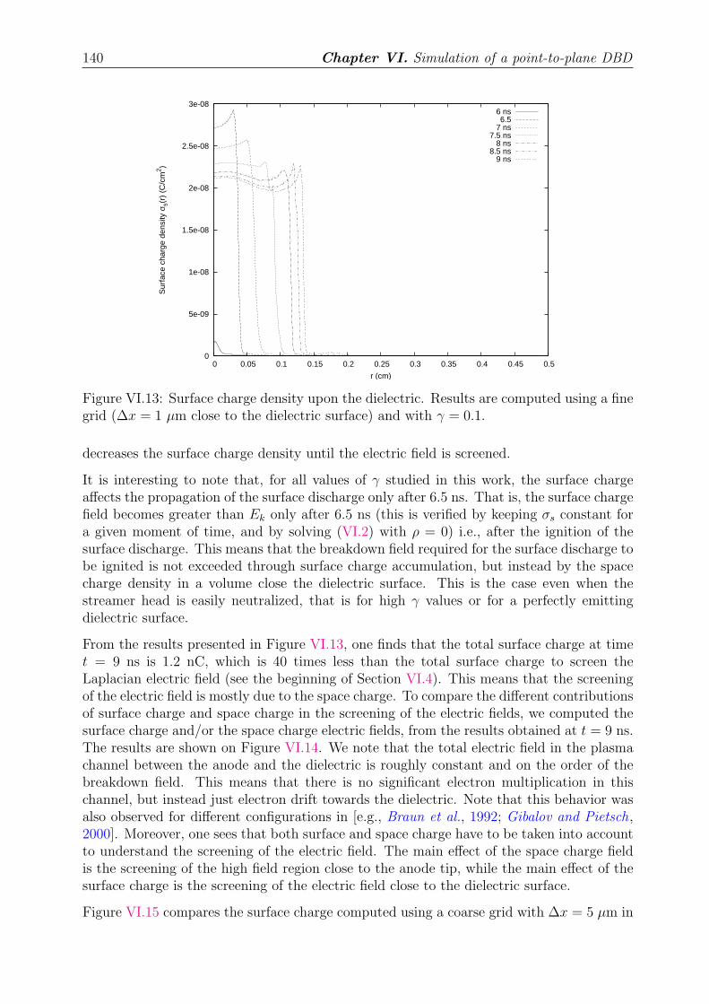
140 Chapter VI. Simulation of a point-to-plane DBD
0
5e-09
1e-08
1.5e-08
2e-08
2.5e-08
3e-08
0 0.05 0.1 0.15 0.2 0.25 0.3 0.35 0.4 0.45 0.5
Sur
face
cha
rge
dens
ity σ
s(r)
(C
/cm
2 )
r (cm)
6 ns6.5
7 ns7.5 ns
8 ns8.5 ns
9 ns
Figure VI.13: Surface charge density upon the dielectric. Results are computed using a finegrid (∆x = 1 µm close to the dielectric surface) and with γ = 0.1.
decreases the surface charge density until the electric field is screened.
It is interesting to note that, for all values of γ studied in this work, the surface chargeaffects the propagation of the surface discharge only after 6.5 ns. That is, the surface chargefield becomes greater than Ek only after 6.5 ns (this is verified by keeping σs constant fora given moment of time, and by solving (VI.2) with ρ = 0) i.e., after the ignition of thesurface discharge. This means that the breakdown field required for the surface discharge tobe ignited is not exceeded through surface charge accumulation, but instead by the spacecharge density in a volume close the dielectric surface. This is the case even when thestreamer head is easily neutralized, that is for high γ values or for a perfectly emittingdielectric surface.
From the results presented in Figure VI.13, one finds that the total surface charge at timet = 9 ns is 1.2 nC, which is 40 times less than the total surface charge to screen theLaplacian electric field (see the beginning of Section VI.4). This means that the screeningof the electric field is mostly due to the space charge. To compare the different contributionsof surface charge and space charge in the screening of the electric fields, we computed thesurface charge and/or the space charge electric fields, from the results obtained at t = 9 ns.The results are shown on Figure VI.14. We note that the total electric field in the plasmachannel between the anode and the dielectric is roughly constant and on the order of thebreakdown field. This means that there is no significant electron multiplication in thischannel, but instead just electron drift towards the dielectric. Note that this behavior wasalso observed for different configurations in [e.g., Braun et al., 1992; Gibalov and Pietsch,2000]. Moreover, one sees that both surface and space charge have to be taken into accountto understand the screening of the electric field. The main effect of the space charge fieldis the screening of the high field region close to the anode tip, while the main effect of thesurface charge is the screening of the electric field close to the dielectric surface.
Figure VI.15 compares the surface charge computed using a coarse grid with ∆x = 5 µm in
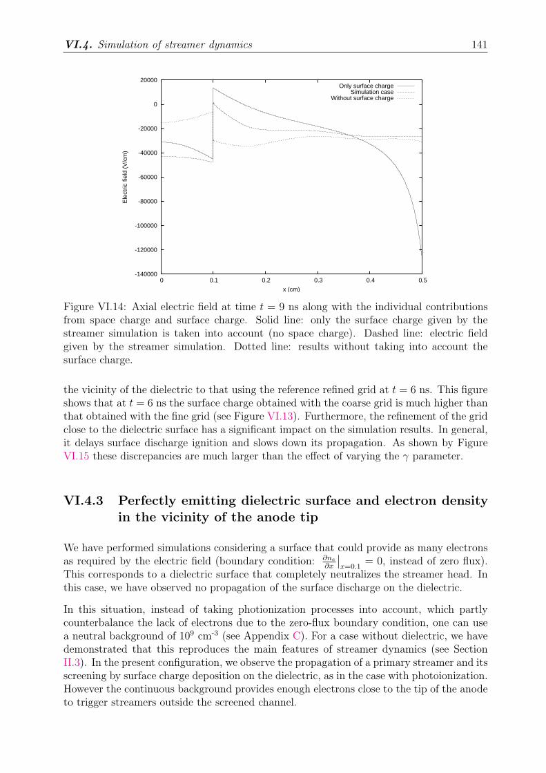
VI.4. Simulation of streamer dynamics 141
-140000
-120000
-100000
-80000
-60000
-40000
-20000
0
20000
0 0.1 0.2 0.3 0.4 0.5
Ele
ctric
fiel
d (V
/cm
)
x (cm)
Only surface chargeSimulation case
Without surface charge
Figure VI.14: Axial electric field at time t = 9 ns along with the individual contributionsfrom space charge and surface charge. Solid line: only the surface charge given by thestreamer simulation is taken into account (no space charge). Dashed line: electric fieldgiven by the streamer simulation. Dotted line: results without taking into account thesurface charge.
the vicinity of the dielectric to that using the reference refined grid at t = 6 ns. This figureshows that at t = 6 ns the surface charge obtained with the coarse grid is much higher thanthat obtained with the fine grid (see Figure VI.13). Furthermore, the refinement of the gridclose to the dielectric surface has a significant impact on the simulation results. In general,it delays surface discharge ignition and slows down its propagation. As shown by FigureVI.15 these discrepancies are much larger than the effect of varying the γ parameter.
VI.4.3 Perfectly emitting dielectric surface and electron densityin the vicinity of the anode tip
We have performed simulations considering a surface that could provide as many electronsas required by the electric field (boundary condition: ∂ne
∂x
∣
∣
x=0.1= 0, instead of zero flux).
This corresponds to a dielectric surface that completely neutralizes the streamer head. Inthis case, we have observed no propagation of the surface discharge on the dielectric.
In this situation, instead of taking photionization processes into account, which partlycounterbalance the lack of electrons due to the zero-flux boundary condition, one can usea neutral background of 109 cm-3 (see Appendix C). For a case without dielectric, we havedemonstrated that this reproduces the main features of streamer dynamics (see SectionII.3). In the present configuration, we observe the propagation of a primary streamer and itsscreening by surface charge deposition on the dielectric, as in the case with photoionization.However the continuous background provides enough electrons close to the tip of the anodeto trigger streamers outside the screened channel.
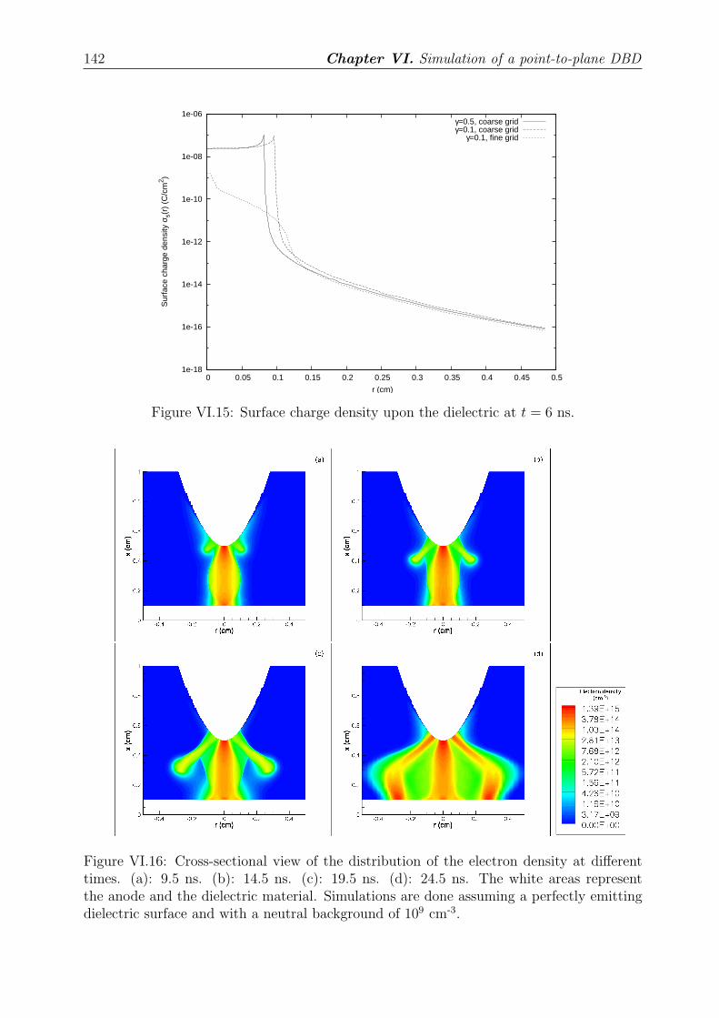
142 Chapter VI. Simulation of a point-to-plane DBD
1e-18
1e-16
1e-14
1e-12
1e-10
1e-08
1e-06
0 0.05 0.1 0.15 0.2 0.25 0.3 0.35 0.4 0.45 0.5
Sur
face
cha
rge
dens
ity σ
s(r)
(C
/cm
2 )
r (cm)
γ=0.5, coarse gridγ=0.1, coarse grid
γ=0.1, fine grid
Figure VI.15: Surface charge density upon the dielectric at t = 6 ns.
Figure VI.16: Cross-sectional view of the distribution of the electron density at differenttimes. (a): 9.5 ns. (b): 14.5 ns. (c): 19.5 ns. (d): 24.5 ns. The white areas representthe anode and the dielectric material. Simulations are done assuming a perfectly emittingdielectric surface and with a neutral background of 109 cm-3.
VI.5. Conclusions 143
Figure VI.16 clearly shows the triggering of the subsequent discharge. Note that the simu-lated discharge is not fully physical, since we use a 2D axisymmetric approach to describea 3D phenomenon. We note that during these simulations the second streamer reaches theexpanding region of the numerical grid, which is the reason for the presence of the smallsquares visible in Figures VI.16(c) and VI.16(d). We presume that this is also the reasonfor the non-physical swelling of the discharge zone visible in Figure VI.16(d). In a full3D simulation, one could expect this secondary discharge to split into several independantstreamers. Moreover, as stated previously, the screening of the electric field on such a shorttime scale (∼10 ns) results from both surface charge and space charge. Conversely, thescreening of the central part of the electric field in the experiment, which determines theparticular shape of filaments corresponding to second current peaks (see Section V.4.2), canonly come from the surface charge trapped on the dielectric. Indeed, the characteristic timebetween two discharges (∼1 ms) is longer than the volume recombination time. However,the surface charge is known to remain for a very long time (see [Golubovskii et al., 2002]for a detailed study of processes related to surface charge upon a dielectric surface). Nev-ertheless, these results show how a second streamer could start from the anode followingthe screening of the electric field by the primary central discharge of a similar radius. Thischaracteristic feature resembles the secondary discharge in the positive half-cycle presentedin Section V.4.2.
VI.5 Conclusions
In this chapter we have simulated a Dielectric Barrier Discharge in a point-to-plane config-uration. Even without space charge in the simulation domain, this configuration is rathercomplex. To define Dirichlet boundary conditions for Poisson’s equation based on an ana-lytical solution, we used a slightly modified geometry with a hyperbolic dielectric interfaceinstead of a plane. We demonstrated that this approximation is accurate, and we suc-cessfully applied it in the framework of streamer modeling via using of the Ghost FluidMethod.
The dynamics of dielectric barrier discharges has been studied, including the initiation of asurface discharge after the propagation of the streamer in the gas gap. We also studied theimportance of the second Townsend coefficient γ, which has been observed to work as anacceleration parameter for the initiation and propagation of the surface discharge. In thesesimulations, we found that the surface discharge initiated by the main streamer starts fromthe space charge close to the dielectric surface and not from an accumulation of surfacecharge. The surface charge plays an important role in the screening of the Laplacian electricfield close to the dielectric, and the space charge contributes significantly to the screeningof the electric field in the vicinity of the anode tip on the considered time scale (∼10 ns).This is why the total charge accumulated on the dielectric surface found in simulations(∼1 nC) is less than the surface charge required to screen the electric field (∼40 nC) (seethe beginning of Section VI.4). We assume that the total charge of 40 nC found in theexperiments (and in our electrostatic studies) corresponds to a surface charge accumulatedover a much longer time.
In this work we have carried out axisymmetric 2D simulations, although a three-dimensionalsimulation would be necessary to simulate the experiment accurately. However, we have

144 Chapter VI. Simulation of a point-to-plane DBD
shown that the screening of the electric field in the channel produced by the initial centralstreamer can influence the subsequent streamers by deflecting them from their expectedtrajectories, as observed in the experiments. In the simulations, the impact radius andthe spatial distribution of the discharge are comparable to the experimental results fromSection V.4.2.
General Conclusion
In this Ph.D. thesis we contribute to several aspects of research on streamer physics in airat atmospheric pressure through both experimental and numerical studies. We show that
studying transient phenomena such as streamer discharges, whose timescales are very shortcompared to the operating times in applications, results in useful informations concerningtheir underlying physical mechanisms.
In this work we have studied streamer dynamics based on the most common and effectivemodel, using drift-diffusion equations for charged species coupled with Poisson’s equation.The numerical resolution of this set of equations requires careful attention to the efficiencyof the numerical schemes used. In fact, it requires making a strict selection of numericalsolvers for the different components of the resolution. The computation of the electricfield is a key point in streamer modeling. First, transport parameters and source terms ofthe drift-diffusion equations have a strongly non-linear dependence on the reduced electricfield. Second, the electric potential itself is directly related to charged species densities viaPoisson’s equation. Thus, to obtain a reliable calculation of the electric field, we have usedtwo different solvers for Poisson’s equation. The first one is an iterative solver based on aNAG library routine. And the second one called SuperLU is a direct solver. Both providevery accurate solutions in all the configurations we tested. Moreover, these solvers are alsoused in the computation of the photoionization processes using the differential approaches.As Poisson’s equation is elliptic, we have carefully defined the boundary conditions for eachcase studied in this work. Numerical methods and schemes used to solve the drift-diffusionequations for charged species have been also described. In this work, we have mainly usedthree different schemes: the simple first-order upwind scheme, the FCT method based on thethe upwind and QUICKEST3 schemes and Zalesak’s limiter, and the modified Scharfetter-Gummel scheme. We showed that the upwind scheme can give the main physical parametersof streamer dynamics. However, it is unable to attain the accuracy of high-order schemeson the considered numerical grids. Thus, to accurately resolve streamer propagation, higherorder schemes such as the FCT method and the modified Scharfetter-Gummel scheme arerequired.
A considerable effort has been to calculate the photoionization process. Indeed, photoion-ization is considered to be of great importance in streamer dynamics in air. The classicalZheleznyak approach, as an integral model, is very time consuming. As a consequence,several differential approaches have been proposed in the literature to reduce the computa-tion time of numerical models for plasma discharges in air. In this work we have developedthree differential approaches: a three-exponential Helmholtz model, a three-group Edding-ton model, and a three-group improved Eddington (SP3) model. The Helmholtz model isbased on approximating of the absorption function of the gas in order to transform theintegral expression of the photoionization term in a set of Helmholtz differential equations.
146 General Conclusion
The Eddington and SP3 methods are based on the direct numerical solution of an approxi-mation of the radiative transfer equation. Finally, we have demonstrated that the solutionsinvolved in all three differential models require accurate definitions of boundary conditions,and we have derived these boundary conditions.
We have carried out comparative studies of these models using mainly two different config-urations for streamer propagation. The homogeneous electric field configuration was usedfor igniting streamers of both polarities propagating in a strong electric field (E>Ek, whereEk is the conventional breakdown field). In this case ionization by electron impact dom-inates over photoionization, where the latter is a second order process. Thus, the choiceof the differential model for calulating the photoionization source term has a small impacton the streamer dynamics. In the other configuration studied, a sphere with high electricpotential lies in an initially weak homogeneous electric field. In this case we studied thepropagation of a streamer in the weak electric field (E<Ek). In this configuration thestreamer dynamics is heavily influenced by the photoionization processes. In this case, wefound that the best agreement with the reference Zheleznyak integral model is obtainedusing the three-group SP3 model. Furthermore, we have shown that the advantage of thethree-group SP3 approach over the three-exponential Helmholtz method is that it providesa purely physical and consistent set of closed equations with the boundary conditions. Theactual advantage of differential models derived in this work over the integral model liesin the simplicity of the implementation of this type of models, and in the unquestionablesimplicity of extending these models to complex two- and three-dimensional simulation ge-ometries. For example, this could involve the propagation of multiple streamer heads in thesame simulation domain and the presence of obstacles in the streamer path (e.g., electrodes,dust particles, aerosols, etc).
In the experiments, electrodes with small radii of curvature are often used in order tolocalize streamer ignition. To take the electrode shapes into account in the simulations, wehave adapted the Ghost Fluid Method to solve Poisson’s equation in order to calculate theelectric potential and field close to the electrode accurately. This method allows us to takethe influence of the exact shape of the electrodes into account in the framework of finitevolume methods using a regular grid, no matter how the electrode surfaces cross the grid.
After having validated the method with classical numerical results of the literature in apoint-to-plane geometry, we carried out simulations in a point-to-point geometry closelylinked with recent experimental results in pre-heated air discharges generated by Nanosec-ond Repetitively Pulsed (NRP) plasmas. We found out that by considering the propagationtimescales of streamers in this configuration, it is possible to draw some conclusions aboutthe final discharge structure (i.e., spark or coronas discharges) which are in good agreementwith the experiments. This also indicates that streamer modeling on short time scales canbe of a great help towards the understanding of nano-pulsed discharges at atmosphericpressure. In particular, this work points out the potential of such a study for finding theranges of parameters allowing for a diffuse regime at atmospheric pressure and ambienttemperature.
Dielectric Barrier Discharges (DBDs) are widely used for industrial applications. At at-mospheric pressure and low frequency (50 Hz), they are mainly constituted of unstablytriggered non-equilibrium transient plasma filaments produced by streamer propagation.In the experimental part of this work, we have studied a particular behavior of plasmafilaments in a DBD during the positive half-cycle of the applied voltage. In the experimen-
General Conclusion 147
tal device close to the point-to-plane configuration studied, the dynamics of discharges hasbeen found to be greatly affected by the surface charge deposited upon the dielectric mate-rial. We have studied the impact of this behavior on the organization of plasma filaments.In such a device, the trapping on long time scales of the charges on the dielectric surface isresponsible for the coupling between subsequent discharges (leading to a substantial currentin the gap during about a hundred nanoseconds) that follows after several milliseconds.
Having gathered the models and methods presented in this Ph.D. thesis, we performedsimulations in a point-to-plane configuration with a dielectric upon the plane cathode inorder to improve the understanding of the behavior experimentally observed in the DBDdevice. In this work we were able to simulate the propagation of the streamer from itsignition point at the anode to the dielectric material, as well as its splitting into surfacedischarges upon reaching the dielectric. We found that the obtained surface discharges arenot ignited by an over-accumulation of charges on the dielectric surface, but rather by aresidual space charge of the streamer head in a thin layer close to the dielectric. We alsofound that the Laplacian electric field quenches on a very short timescale (<10 ns) becauseof both the contribution of the accumulated surface charge and the residual space chargein the streamer channel. On such time scales the surface charge contributes mainly tothe screening of the electric field close to the dielectric, while the space charge contributesmainly to the screening of the field close to the anode. From the perspective to this study, itwould be interesting to analyze the decrease of the current along with the related transportof charges and to study several amplitudes of the applied voltage.
Considering the time scales of the applied voltage at low frequency, the space charge nec-essarily disappears in the during the time between two subsequent discharges observedexperimentally. Furthermore the surface charge found in simulations for time scales ofabout 10 ns is not sufficient to screen the electric field by itself. Thus, we assumed that themajor part of the surface charge is accumulated on a much longer timescale, correspondingto the decrease of the current peak found in the measurements (∼100 ns). We also observedthat the increased population of electrons in the vicinity of the anode allows for the ignitionof subsequent streamers. The propagation of these streamers is deflected because of thescreening of the electric field, which is in agreement with experimental observations.

Suggestions for future research
It has been demonstrated in this work that fluid simulations of streamers in complex electricfields configurations represents a very interesting potential concerning the prediction of thedifferent regimes in NRPs. From this perspective, it is important to check the influenceof initial and external conditions on the simulation results. For example, studying theeffects of the radius of curvature and the pre-ionized background on the discharge dynamicswould allow us to verify the consistency of simulation results1. To determine the spatialdistribution of pre-ionized background just before a new discharge more accurately, it wouldbe very interesting to simulate the spatio-temporal distribution of charged species in thepost-discharge. Furthermore, it would be interesting to obtain additional results on thevoltage ranges of the diffuse regime (as a function of the temperature) and to analyzethem carefully to differentiate this regime from the corona and spark regimes. It wouldbe also interesting to take the increase of the neutral gas temperature into account inthe simulations, especially for determining the range of applied voltages for obtaining sparkdischarges accurately. As an extensive experimental work has been done on the spectroscopyof the discharge at 1000 K, it would be of great interest to compute (at least as a post-treatment of simulation results) the excited states densities and to compare them with theexperimental results, especially the observation of wave propagation in the diffuse regime.Finally, it would be interesting to simulate successive discharges to study synergy effectsat high frequency. In the future, the challenge is to couple these simulations with Navier-Stokes flow codes to study the plasma/flow interaction which is of great importance forapplications such as plasma-assisted combustion or flow control.
Considering the DBD studies, experimental studies (not shown in this thesis) have shownthat negative discharges occurring in the considered experimental device are much morediffuse than the positive ones. In the future, it would be interesting to simulate this behaviorand to obtain the shape of the surface charge produced by such a discharge. In this work, wehave considered simplified boundary conditions with a global γ coefficient at the dielectricplane. It would be interesting to model surface processes in the simulations by takinginto account photoemission, recharging of ions, thermal influence, etc. Furthermore, inthis work we have simulated only one discharge assuming a constant applied voltage. Itwould be interesting to simulate the discharge during several cycles of the applied voltageto understand the role of surface charges on long timescales better.
Concerning the theoretical approach on streamer dynamics, many questions remain open.Some of them have been summarized in [Pasko, 2006]. For example, stability and branching
1At the time of publishing this thesis, one parametric study on the radius of curvature [Blackmond et al.,NSF EE REU Penn State Annual Research Journal, Vol. VII, 2009] and one study about the pre-ionizedbackground [Bourdon et al., accepted for publication in PSST, 2009] have been already carried out in thesame configuration.

150 Suggestions for future research
of streamers remain unsolved problems. It is obvious that a better theoretical understandingof the streamer dynamics would lead to great improvements in the conception of newreactors, as well as in the understanding of natural phenomenon involving streamers.
Appendix A
Accuracy of different photoionizationmodels for different simulationdomain dimensions and boundaryconditions
Figure A.1 presents the same information as Figure III.5, only for the domain dimension2×2 cm2 with σ=0.1 cm.
Figures A.1(a) and A.1(b) show the axial and radial profiles of the photoionization sourceterm Sph calculated by the Zheleznyak model in comparison with the Helmholtz solutionsobtained using the two and three-exponential fits. As in Figure III.5, the ionization termSi is also shown for reference. The results obtained with the three-exponential fit appearto match better with the Zheleznyak integral solution in the region where Sph>Si and, inparticular, close to the boundaries. The two-exponential Helmholtz model fails to providean accurate solution in this case. This result directly relates to a poor two-exponential fitat large pO2
R>60 Torr cm values (i.e., R>0.5 cm at ground pressure considered here), ascan be seen in Figure III.2. The better performance of the three-exponential Helmholtzmodel directly relates to a better three-exponential fit at large pO2
R values (i.e., R>0.5 cmat ground pressure), as also can be seen in Figure III.2.
Figures A.1(c) and A.1(d) compare the 3-group Eddington approximation and the 3-groupSP3 with the Zheleznyak model for the same domain dimension 2×2 cm2. We note that theuse of the SP3 allows to improve the agreement with the Zheleznyak model, in particular,close to the boundaries.
Finally, Figures A.1(e) and A.1(f) compare the 3-group SP3 and the 3-exponential Helmholtzmodel with the Zheleznyak model. In this case, both models give very similar results inthe axial direction and are very close to the Zheleznyak model. In the radial direction,the results obtained with the SP3 model appear to be slightly more accurate than thethree-exponential Helmholtz model in the region where Sph>Si.
As we emphasized at the beginning Section III.6.1, for the domain with Ld=Rd the effectivedistance from the source at the center of the simulation domain to the boundary is twotimes longer in the radial direction than in the axial direction (i.e., 2 cm versus 1 cm inFigure A.1). Therefore the radial distances exceeding 1 cm allow to observe the behavior
152 Appendix A. Accuracy of different photoionization models
of different models in the region beyond applicability of the model fits obtained for therange 1<pO2
R<150 Torr cm for the three-exponential Helmholtz model (Figure III.2) andfor 0.1<pO2
R<150 Torr cm for the three-group Eddington and SP3 models (Figure III.3)(i.e., for R<1 cm at atmospheric pressure pO2
=150 Torr). All models shown in FiguresA.1(e) and A.1(f) show outstanding performance in both axial and radial directions atdistances <1 cm from the source, as expected from the range of validity of related fits inFigures III.2 and III.3. In the same vein we note that a special caution should be usedwhen models described in the present work are applied in large simulation domains forwhich pO2
R product exceeds 150 Torr cm.
Figure A.2 is presented in the same format as Figures III.5 and A.1, only for the domaindimension 0.02×0.02 cm2 with σ=0.001 cm.
Figures A.2(a) and A.2(b) show the axial and radial profiles of the photoionization sourceterm Sph calculated by the Zheleznyak model and the Helmholtz solution using two andthree-exponential fits. As expected from the fits shown in Figure III.2 for small distances,the results obtained with both solutions are poor, but we note that in the region of interestfor streamer simulations (where Sph>Si), the three-exponential Helmhotz model appearsto be in a relatively good agreement with the Zheleznyak model.
In Figures A.2(c) and A.2(d), we compare the three-group Eddington approximation andthe three-group SP3 with the Zheleznyak model. We note that the use of the SP3 allowsto improve the agreement with the Zheleznyak model, in particular, in the region whereSph>Si.
In Figures A.2(e) and A.2(f), we compare the three-group SP3 and the three-exponentialHelmholtz model with the Zheleznyak model. In this case, in the region where Sph>Si bothmodels give very similar results in the axial direction and are very close to the Zheleznyakmodel. In the radial direction, the results obtained with the SP3 model appear to be slightlymore accurate than the three-exponential Helmholtz model in the region where Sph>Si.
Figures A.3(a) and A.3(b) demonstrate comparative performance of the boundary condi-tions specified by equations (III.29) or (III.31) using the three-group SP3 approximation fordomain dimensions 2×2 cm2 and σ=0.1 cm. The results are in very good agreement withthe results of the Zheleznyak model. Nevertheless, one can note that the use of equation(III.31) slightly overestimates the exact value of the photoionization source term at theboundaries in the radial direction, but the agreement is good in the axial direction. InFigures A.3(c) and A.3(d) which present computations for a domain dimension 0.02×0.02cm2 and σ=0.001 cm, the use of equation (III.31) for defining boundary conditions slightlyoverestimates the exact value of the photoionization source term at the boundaries in boththe axial and radial directions.
Figures A.4(a) and A.4(b) correspond to the domain dimension 0.02×0.02 cm2 with σ=0.001cm. In this case, the use of equation (III.30) slightly overestimates the exact value of thephotoionization source term at the boundaries in both the axial and radial directions,although for the domain dimension 2×2 cm2 with σ=0.1 cm (Figures A.4(e) and A.4(f))the photoionization source term at the boundaries in both the axial and radial directionsis underestimated.
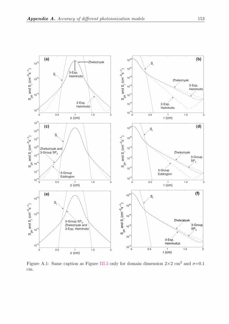
Appendix A. Accuracy of different photoionization models 153
0 0.5 1 1.5 2
1016
1018
1020
1022
z (cm)
Sp
h a
nd
Si (
cm
−3s
−1)
(a)
Si
3-Exp.
Helmholtz
2-Exp.
Helmholtz
Zheleznyak
0 0.5 1 1.5 210
10
1012
1014
1016
1018
1020
1022
r (cm)
Sp
h a
nd
Si (
cm
−3s
−1)
(b)S
i
3-Exp.
Helmholtz
2-Exp.
Helmholtz
Zheleznyak
0 0.5 1 1.5 210
16
1017
1018
1019
1020
1021
1022
1023
z (cm)
Sp
h a
nd S
i (cm
−3s
−1)
(c)
3-Group
Eddington
Zheleznyak and
3-Group SP3
Si
0 0.5 1 1.5 2
1012
1014
1016
1018
1020
1022
r (cm)
Sp
h a
nd S
i (cm
−3s
−1)
(d)S
i
3-Group
SP3
3-Group
Eddington
Zheleznyak
0 0.5 1 1.5 2
1016
1018
1020
1022
z (cm)
Sp
h a
nd S
i (cm
−3s
−1)
(e)
Si
3-Group SP3,
Zheleznyak and
3-Exp. Helmholtz
0 0.5 1 1.5 210
12
1014
1016
1018
1020
1022
r (cm)
Sph a
nd S
i (cm(5
s(3
)
(f)S
i
5/Gzr0"Helmholtz
Zheleznyak
5/ItqwrSP5
Figure A.1: Same caption as Figure III.5 only for domain dimension 2×2 cm2 and σ=0.1cm.
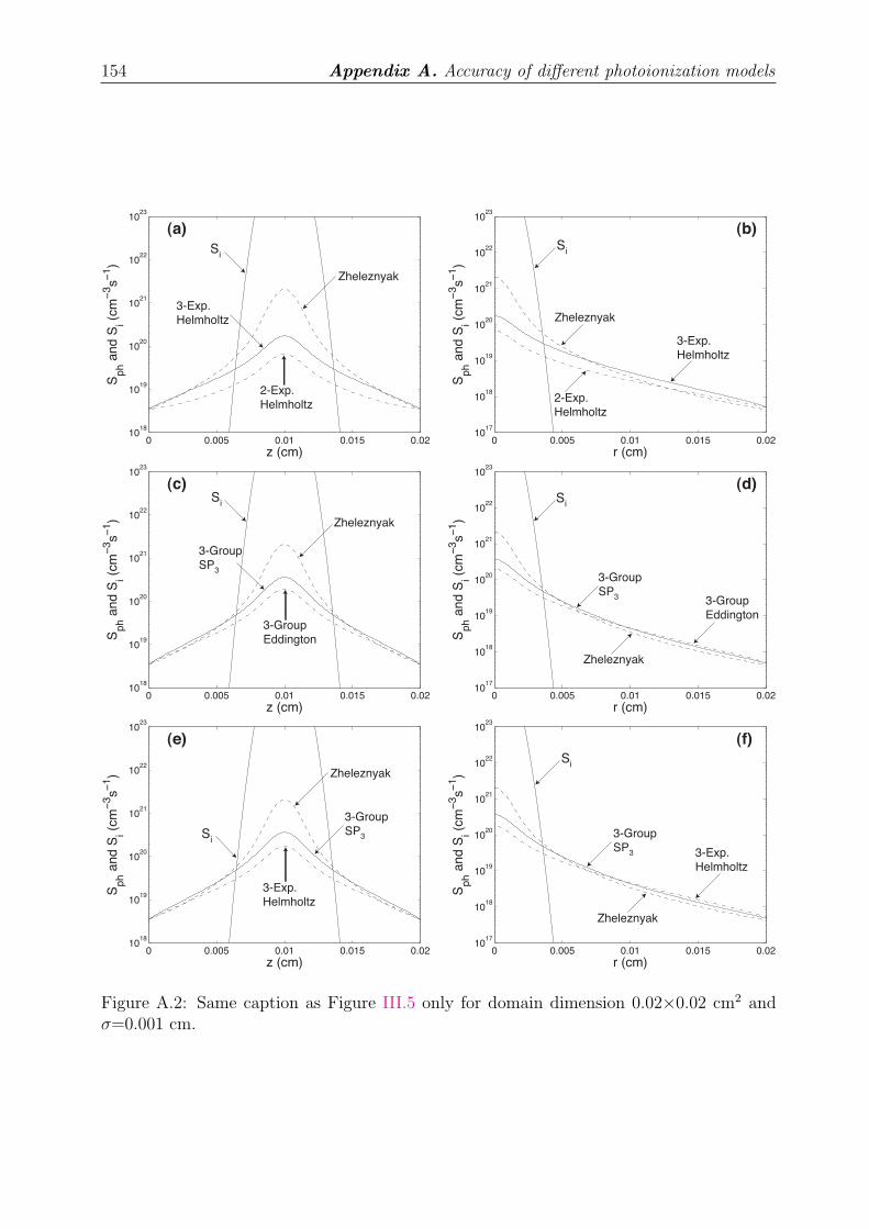
154 Appendix A. Accuracy of different photoionization models
0 0.005 0.01 0.015 0.0210
18
1019
1020
1021
1022
1023
z (cm)
Sp
h a
nd
Si (
cm
−3s
−1)
(a)
Si
3-Exp.
Helmholtz
2-Exp.
Helmholtz
Zheleznyak
0 0.005 0.01 0.015 0.0210
17
1018
1019
1020
1021
1022
1023
r (cm)S
ph a
nd
Si (
cm
−3s
−1)
(b)S
i
3-Exp.
Helmholtz
2-Exp.
Helmholtz
Zheleznyak
0 0.005 0.01 0.015 0.0210
18
1019
1020
1021
1022
1023
z (cm)
Sp
h a
nd S
i (cm
−3s
−1)
(c)S
i
3-Group
SP3
3-Group
Eddington
Zheleznyak
0 0.005 0.01 0.015 0.0210
17
1018
1019
1020
1021
1022
1023
r (cm)
Sp
h a
nd S
i (cm
−3s
−1)
(d)S
i
3-Group
SP3 3-Group
Eddington
Zheleznyak
0 0.005 0.01 0.015 0.0210
18
1019
1020
1021
1022
1023
z (cm)
Sp
h a
nd S
i (cm
−3s
−1)
(e)
Si
3-Exp.
Helmholtz
Zheleznyak
3-Group
SP3
0 0.005 0.01 0.015 0.0210
17
1018
1019
1020
1021
1022
1023
r (cm)
Sp
h a
nd S
i (cm
−3s
−1)
(f)
Si
3-Exp.
Helmholtz
Zheleznyak
3-Group
SP3
Figure A.2: Same caption as Figure III.5 only for domain dimension 0.02×0.02 cm2 andσ=0.001 cm.
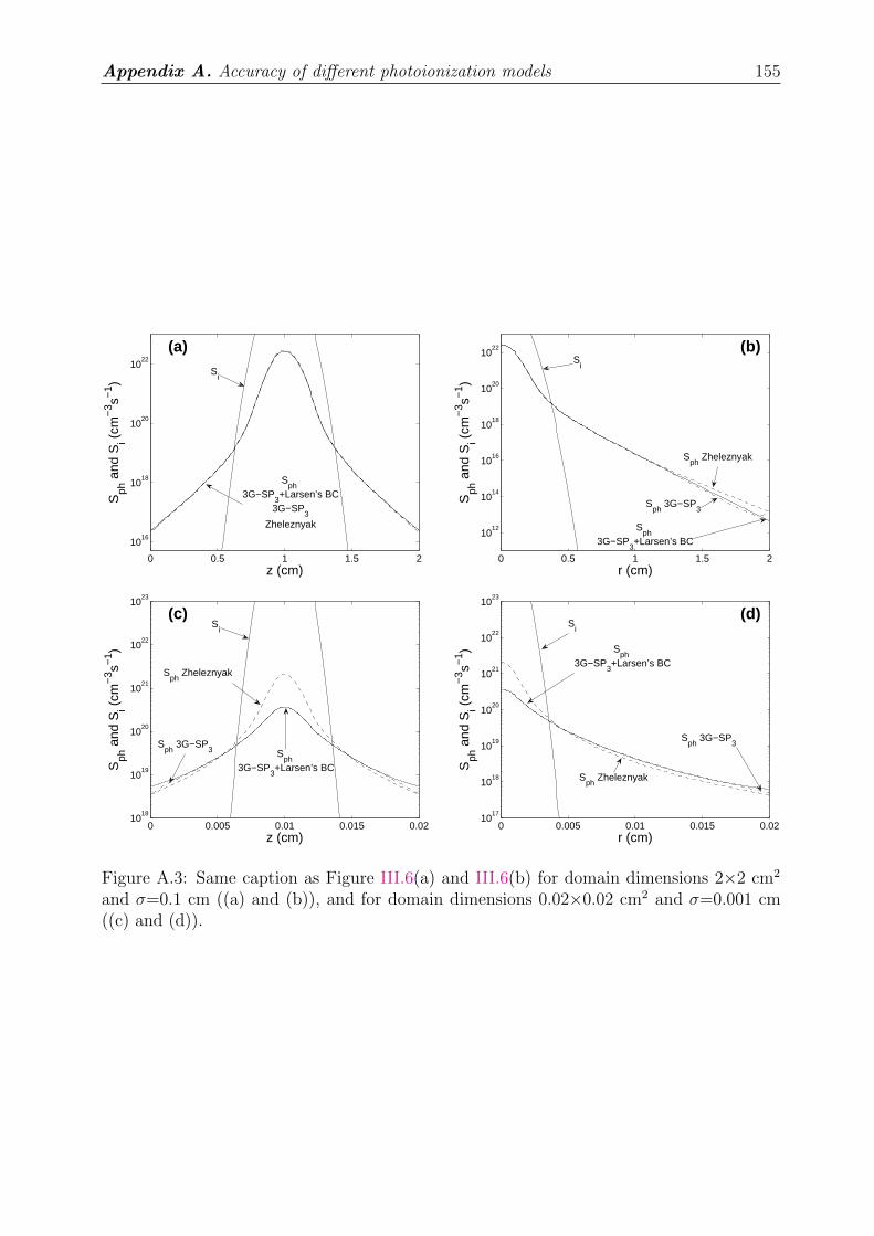
Appendix A. Accuracy of different photoionization models 155
0 0.5 1 1.5 2
1016
1018
1020
1022
z (cm)
Sph
and
Si (
cm−
3 s−1 )
(a)S
i
Sph
3G−SP
3+Larsen’s BC
3G−SP3
Zheleznyak
0 0.5 1 1.5 2
1012
1014
1016
1018
1020
1022
r (cm)
Sph
and
Si (
cm−
3 s−1 )
(b)S
i
Sph
Zheleznyak
Sph
3G−SP3
Sph
3G−SP
3+Larsen’s BC
0 0.005 0.01 0.015 0.0210
18
1019
1020
1021
1022
1023
z (cm)
Sph
and
Si (
cm−
3 s−1 )
(c)
Sph
Zheleznyak
Si
Sph
3G−SP3 S
ph
3G−SP3+Larsen’s BC
0 0.005 0.01 0.015 0.0210
17
1018
1019
1020
1021
1022
1023
r (cm)
Sph
and
Si (
cm−
3 s−1 )
(d)S
i
Sph
3G−SP
3+Larsen’s BC
Sph
Zheleznyak
Sph
3G−SP3
Figure A.3: Same caption as Figure III.6(a) and III.6(b) for domain dimensions 2×2 cm2
and σ=0.1 cm ((a) and (b)), and for domain dimensions 0.02×0.02 cm2 and σ=0.001 cm((c) and (d)).
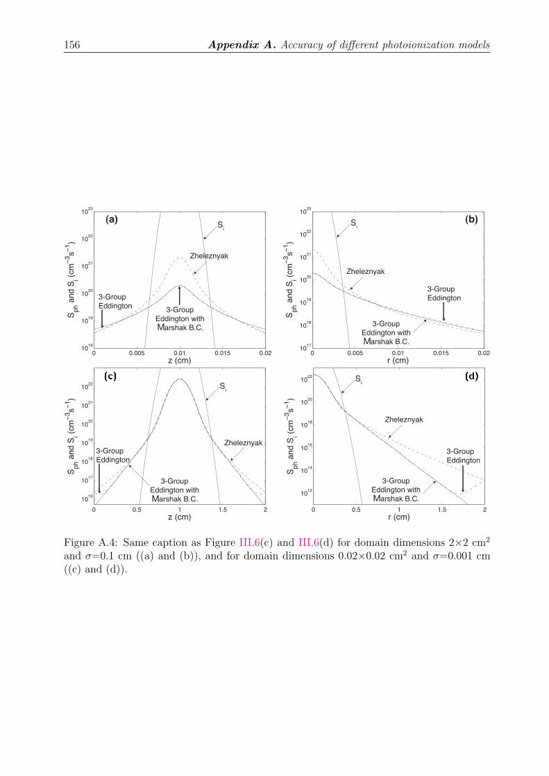
156 Appendix A. Accuracy of different photoionization models
0 0.005 0.01 0.015 0.0210
18
1019
1020
1021
1022
1023
z (cm)
Sp
h a
nd
Si (
cm
−3s
−1)
(a)S
i
Zheleznyak
3-Group
Eddington3-Group
Eddington with
arshak B.C.
0 0.005 0.01 0.015 0.0210
17
1018
1019
1020
1021
1022
1023
r (cm)
Sp
h a
nd
Si (
cm
−3s
−1)
(b)Si
Zheleznyak
3-Group
Eddington
3-Group
Eddington with
arshak B.C.
0 0.5 1 1.5 2
1016
1017
1018
1019
1020
1021
1022
z (cm)
Sp
h a
nd S
i (cm
−3s
−1)
(e)S
i
Zheleznyak3-Group
Eddington
3-Group
Eddington with
arshak B.C.
0 0.5 1 1.5 2
1012
1014
1016
1018
1020
1022
r (cm)
Sp
h a
nd S
i (cm
−3s
−1)
(f)Si
Zheleznyak
3-Group
Eddington
3-Group
Eddington with
arshak B.C.
M
M
M M
Figure A.4: Same caption as Figure III.6(c) and III.6(d) for domain dimensions 2×2 cm2
and σ=0.1 cm ((a) and (b)), and for domain dimensions 0.02×0.02 cm2 and σ=0.001 cm((c) and (d)).
Appendix B
Mathematical relationships betweenthe Eddington, SP3 and Helmholtzmodels
Some results of this appendix have been published in [Bourdon et al., 2007].
The three-group Eddington and SP3 models presented in Chapter III have been derived onphysical grounds from the general radiative transfer equation. These physics based modelshave certain advantages in comparison with the Helmholtz model, allowing in particular toformulate a consistent and computationally efficient set of equations and boundary condi-tions based on a radiative transfer theory (see Section III.4). It is useful, however, to bringto attention of the readers that the equation (III.20) of the Eddington model and equations(III.21) and (III.22) of the SP3 model are Helmholtz equations. Therefore, as demonstratedbelow in this Appendix, for these equations it is possible to derive effective representationsof the g(R)/pO2
function of the type specified by equation (III.9) of the Helmholtz modeldescribed in Section III.3. The establishment of these mathematical relationships betweenEddington, SP3 and Helmholtz models is very useful for interpretation of results presentedin Section III.6.1, and evaluation of performance of the Eddington and SP3 models in thegeneral context of the quality of the fit of the g(R)/pO2
function given by equation (III.9)in comparison with the original g(R)/pO2
function of the Zheleznyak photoionization modelspecified by equation (III.3).
Each of the Helmholtz differential equations (III.8) is similar to equations for wave potentialscommonly encountered in antenna theory in electromagnetics [Harrington, 2001; Landauand Lifshitz , 1971, Chapter VIII, § 64]. On a conceptual level the electromagnetic problemcorresponds to a case of purely imaginary λj values for which the equation (III.7) wouldrepresent outgoing waves [Harrington, 2001, p. 80]. In the photoionization problem the λj
values are real, reflecting exponential spatial damping of the solutions due to the absorptionof the photoionizing radiation. The appearance of the similar Helmholtz equations (III.20),(III.21) and (III.22) in the Eddington and improved Eddington approximations to theradiative transfer equation is also consistent with the above physical interpretation. In thisAppendix we demonstrate that the solutions of the Helmholtz, Eddington and SP3 modelscan be represented in a mathematically equivalent form, however, all represent approximatesolutions of the same problem, rely on different numerical values of the model coefficients,and therefore generally do not lead to identical results.
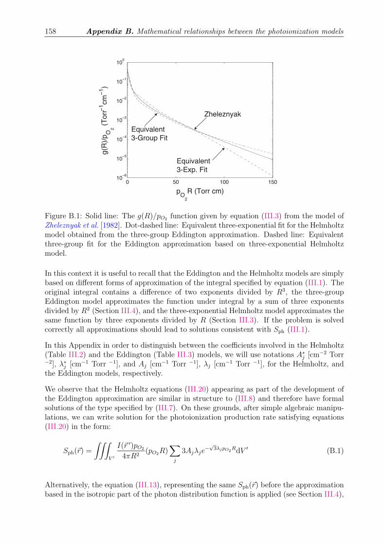
158 Appendix B. Mathematical relationships between the photoionization models
0 50 100 15010
−6
10−5
10−4
10−3
10−2
10−1
100
pO2
R (Torr cm)
g(R)/pO2
(Torr−1cm−1)
Zheleznyak
Equivalent
3-Exp. Fit
Equivalent
3-Group Fit
Figure B.1: Solid line: The g(R)/pO2function given by equation (III.3) from the model of
Zheleznyak et al. [1982]. Dot-dashed line: Equivalent three-exponential fit for the Helmholtzmodel obtained from the three-group Eddington approximation. Dashed line: Equivalentthree-group fit for the Eddington approximation based on three-exponential Helmholtzmodel.
In this context it is useful to recall that the Eddington and the Helmholtz models are simplybased on different forms of approximation of the integral specified by equation (III.1). Theoriginal integral contains a difference of two exponents divided by R3, the three-groupEddington model approximates the function under integral by a sum of three exponentsdivided by R2 (Section III.4), and the three-exponential Helmholtz model approximates thesame function by three exponents divided by R (Section III.3). If the problem is solvedcorrectly all approximations should lead to solutions consistent with Sph (III.1).
In this Appendix in order to distinguish between the coefficients involved in the Helmholtz(Table III.2) and the Eddington (Table III.3) models, we will use notations A∗
j [cm−2 Torr−2], λ∗
j [cm−1 Torr −1], and Aj [cm−1 Torr −1], λj [cm−1 Torr −1], for the Helmholtz, andthe Eddington models, respectively.
We observe that the Helmholtz equations (III.20) appearing as part of the development ofthe Eddington approximation are similar in structure to (III.8) and therefore have formalsolutions of the type specified by (III.7). On these grounds, after simple algebraic manipu-lations, we can write solution for the photoionization production rate satisfying equations(III.20) in the form:
Sph(~r) =
∫∫∫
V ′
I(~r ′)pO2
4πR2(pO2
R)∑
j
3Ajλje−√
3λjpO2RdV ′ (B.1)
Alternatively, the equation (III.13), representing the same Sph(~r) before the approximationbased in the isotropic part of the photon distribution function is applied (see Section III.4),
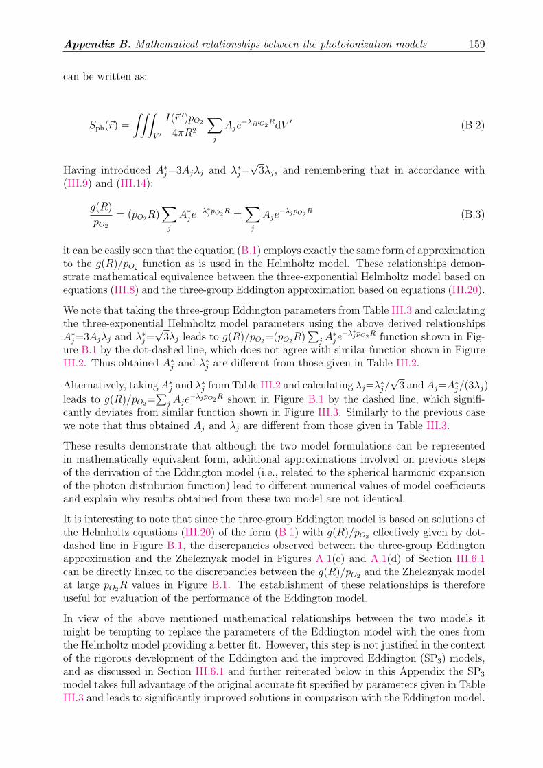
Appendix B. Mathematical relationships between the photoionization models 159
can be written as:
Sph(~r) =
∫∫∫
V ′
I(~r ′)pO2
4πR2
∑
j
Aje−λjpO2
RdV ′ (B.2)
Having introduced A∗j=3Ajλj and λ∗
j=√
3λj, and remembering that in accordance with(III.9) and (III.14):
g(R)
pO2
= (pO2R)∑
j
A∗je
−λ∗
j pO2R =
∑
j
Aje−λjpO2
R (B.3)
it can be easily seen that the equation (B.1) employs exactly the same form of approximationto the g(R)/pO2
function as is used in the Helmholtz model. These relationships demon-strate mathematical equivalence between the three-exponential Helmholtz model based onequations (III.8) and the three-group Eddington approximation based on equations (III.20).
We note that taking the three-group Eddington parameters from Table III.3 and calculatingthe three-exponential Helmholtz model parameters using the above derived relationshipsA∗
j=3Ajλj and λ∗j=
√3λj leads to g(R)/pO2
=(pO2R)∑
j A∗je
−λ∗
j pO2R function shown in Fig-
ure B.1 by the dot-dashed line, which does not agree with similar function shown in FigureIII.2. Thus obtained A∗
j and λ∗j are different from those given in Table III.2.
Alternatively, taking A∗j and λ∗
j from Table III.2 and calculating λj=λ∗j/√
3 and Aj=A∗j/(3λj)
leads to g(R)/pO2=∑
j Aje−λjpO2
R shown in Figure B.1 by the dashed line, which signifi-cantly deviates from similar function shown in Figure III.3. Similarly to the previous casewe note that thus obtained Aj and λj are different from those given in Table III.3.
These results demonstrate that although the two model formulations can be representedin mathematically equivalent form, additional approximations involved on previous stepsof the derivation of the Eddington model (i.e., related to the spherical harmonic expansionof the photon distribution function) lead to different numerical values of model coefficientsand explain why results obtained from these two model are not identical.
It is interesting to note that since the three-group Eddington model is based on solutions ofthe Helmholtz equations (III.20) of the form (B.1) with g(R)/pO2
effectively given by dot-dashed line in Figure B.1, the discrepancies observed between the three-group Eddingtonapproximation and the Zheleznyak model in Figures A.1(c) and A.1(d) of Section III.6.1can be directly linked to the discrepancies between the g(R)/pO2
and the Zheleznyak modelat large pO2
R values in Figure B.1. The establishment of these relationships is thereforeuseful for evaluation of the performance of the Eddington model.
In view of the above mentioned mathematical relationships between the two models itmight be tempting to replace the parameters of the Eddington model with the ones fromthe Helmholtz model providing a better fit. However, this step is not justified in the contextof the rigorous development of the Eddington and the improved Eddington (SP3) models,and as discussed in Section III.6.1 and further reiterated below in this Appendix the SP3
model takes full advantage of the original accurate fit specified by parameters given in TableIII.3 and leads to significantly improved solutions in comparison with the Eddington model.
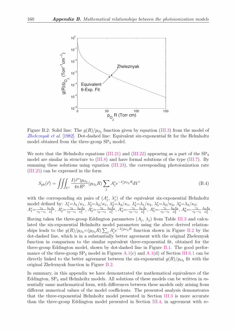
160 Appendix B. Mathematical relationships between the photoionization models
0 50 100 15010
−6
10−5
10−4
10−3
10−2
10−1
100
pO2
R (Torr cm)
g(R)/pO2
(Torr−1cm−1)
Zheleznyak
Equivalent
6-Exp. Fit
Figure B.2: Solid line: The g(R)/pO2function given by equation (III.3) from the model of
Zheleznyak et al. [1982]. Dot-dashed line: Equivalent six-exponential fit for the Helmholtzmodel obtained from the three-group SP3 model.
We note that the Helmholtz equations (III.21) and (III.22) appearing as a part of the SP3
model are similar in structure to (III.8) and have formal solutions of the type (III.7). Bysumming these solutions using equation (III.23), the corresponding photoionization rate(III.25) can be expressed in the form
Sph(~r) =
∫∫∫
V ′
I(~r ′)pO2
4πR2(pO2
R)∑
j
A∗je
−λ∗
j pO2RdV ′ (B.4)
with the corresponding six pairs of (A∗j , λ∗
j) of the equivalent six-exponential Helmholtzmodel defined by: λ∗
1=λ1/κ1, λ∗2=λ2/κ1, λ∗
3=λ3/κ1, λ∗4=λ1/κ2, λ∗
5=λ2/κ2, λ∗6=λ3/κ2;
A∗1=
γ2
γ2−γ1
λ1A1
κ21
, A∗2=
γ2
γ2−γ1
λ2A2
κ21
, A∗3=
γ2
γ2−γ1
λ3A3
κ21
, A∗4=- γ1
γ2−γ1
λ1A1
κ22
, A∗5=- γ1
γ2−γ1
λ2A2
κ22
, A∗6=- γ1
γ2−γ1
λ3A3
κ22
.
Having taken the three-group Eddington parameters (Aj, λj) from Table III.3 and calcu-lated the six-exponential Helmholtz model parameters using the above derived relation-ships leads to the g(R)/pO2
=(pO2R)∑
j A∗je
−λ∗
j pO2R function shown in Figure B.2 by the
dot-dashed line, which is in a substantially better agreement with the original Zheleznyakfunction in comparison to the similar equivalent three-exponential fit, obtained for thethree-group Eddington model, shown by dot-dashed line in Figure B.1. The good perfor-mance of the three-group SP3 model in Figures A.1(c) and A.1(d) of Section III.6.1 can bedirectly linked to the better agreement between the six-exponential g(R)/pO2
fit with theoriginal Zheleznyak function in Figure B.2.
In summary, in this appendix we have demonstrated the mathematical equivalence of theEddington, SP3 and Helmholtz models. All solutions of these models can be written in es-sentially same mathematical form, with differences between these models only arising fromdifferent numerical values of the model coefficients. The presented analysis demonstratesthat the three-exponential Helmholtz model presented in Section III.3 is more accuratethan the three-group Eddington model presented in Section III.4, in agreement with re-

Appendix B. Mathematical relationships between the photoionization models 161
sults presented in Section III.6.1. The presented analysis also demonstrates that the SP3
model can be effectively represented in a mathematical form equivalent to six-exponentialHelmholtz model. This approach allows a simple interpretation of better performance of thethree-group SP3 model in comparison with the three-group Eddington model introduced inSection III.4, and in comparison with the three-exponential Helmholtz model presented inSection III.4, in agreement with the results presented in Section III.6.1.


Appendix C
Determination of the pre-ionizationlevel for streamer propagation inweak field at ground pressure in air
Using an initial continuous neutral pre-ionization level instead of the full model for pho-toionization is a simple way to save computation time. Obviously, the important point isthen the determination of the pre-ionization level. In this appendix, we develop an approachto determine this pre-ionization level.
Pancheshnyi et al. [2001] have mentioned that it is possible to attain the coincidence of somecharacteristics (but not for all the characteristics simultaneously) of streamer discharges,by varying the level of pre-ionization background. To avoid doing systematic parametricstudies with different pre-ionization levels, in this appendix, we determine the level of pre-ionization based on the dynamics of the streamer head. This analysis is based on thesimulation results obtained with the full model for photoionization. Figure C.1 shows thedirect ionization by electron impact rate, the photoionization rate, and the electron densityat time t = 17.5 ns in the simulation case of streamer propagation in a weak field depictedin Section III.6.2 and computed using the FCT+QUICKEST3 scheme (see Chapter II).
As mentioned in Chapter III, the ionization rate is higher than the photoionization rate inthe narrow region of the streamer head. Behind this region, in the streamer channel, thephotoionization rate is higher than the ionization rate. In front of the streamer head, wherethe gas is still mainly neutral, the creation of electrons and ions mainly results from thephotoionization process beyond the intersection point of the ionization and photoionizationrates. In Figure C.1 at time t = 17.5 ns one can say that the creation of seed electrons ismainly governed by photoionization in the region x & 0.77 cm.
Moreover, the electron density which corresponds to the location of equal ionization andphotoionization rates, is quite constant during stable streamer propagation. We concludedthat this value of the electron density, which is negligible compared to the density inside thestreamer channel, can be interpreted as the electron density mainly produced by photoion-ization at this location. Considering the impact of photoionization on the local dynamicsof the head, this value could replace the seed electrons due to photoionization in front ofthe streamer head. In the case of Figure C.1 this value is ∼109 cm-3.
We have checked this method in different configurations and we observed that it is efficient
164 Appendix C. Determination of the pre-ionization level
❯
Electron density
Photoionization rate
PPPqIonization rate
1e+08
1e+10
1e+12
1e+14
1e+16
1e+18
1e+20
1e+22
1e+24
0 0.1 0.2 0.3 0.4 0.5 0.6 0.7 0.8 0.9 1 1e+06
1e+07
1e+08
1e+09
1e+10
1e+11
1e+12
1e+13
1e+14
1e+15
Sou
rce
term
rat
es (
cm-3
.s-1
)
Ele
ctro
n de
nsity
(cm
-3)
x (cm)
Figure C.1: Photoionization and direct ionization rates, and electron density at time t =17.5 ns for the streamer propagation in a weak field presented in Section III.6.2.
to find a good approximation of the pre-ionization level.
Figures C.2 and C.3 show the comparison of the electron densities and axial electric field,respectively, between the simulations using either a pre-ionization background or the com-putation of the photoionization source term. In the cases without photoionization weconsidered the pre-ionization levels of 109 cm-3 and 1010 cm-3. For a pre-ionization level of108 cm-3, we have not observed any streamer propagation.
Figure C.2 shows that the pre-ionization level of 109 cm-3 gives a good agreement withthe computation of the photoionization source term. The electron density in the channelis in very good agreement, as well as the electric field in the streamer channel showedby Figure C.3. The electric field in the streamer head is also well described. The maindifference between the case with the pre-ionization level at 109 cm-3 and the case withthe computation of the photoionization source term is the propagation velocity, which is aslightly higher when the photoionization source term is calculated.
One can also note that with a pre-ionization level of 1010 cm-3, the propagation of thestreamer is slower in spite of relation (I.13). This means that increasing the pre-ionizedbackground does not have a simple impact on the streamer dynamics and leads, for example,to a non-negligible change of the electric field (see Figure C.3). To argue in this direction, wealso noted that, at the beginning of the propagation, for the pre-ionized case at 1010 cm-3 thestreamer is faster than for the other cases, but streamers calculated using photoionizationmodel and 109 cm-3 pre-ionization pass it at about 12 ns.
In conclusion, we have shown that to reproduce the streamer propagation in the weak fieldcase presented in Section III.6.2, a pre-ionization level of 109 cm-3 gives a good agreement
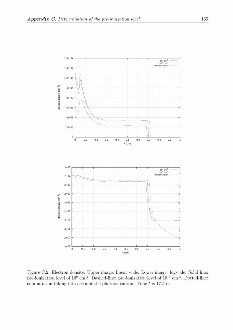
Appendix C. Determination of the pre-ionization level 165
0
2e+13
4e+13
6e+13
8e+13
1e+14
1.2e+14
1.4e+14
1.6e+14
0 0.1 0.2 0.3 0.4 0.5 0.6 0.7 0.8 0.9 1
Ele
ctro
n de
nsity
(cm
-3)
x (cm)
109 cm-3
1010 cm-3
Photoionization
1e+06
1e+07
1e+08
1e+09
1e+10
1e+11
1e+12
1e+13
1e+14
1e+15
0 0.1 0.2 0.3 0.4 0.5 0.6 0.7 0.8 0.9 1
Ele
ctro
n de
nsity
(cm
-3)
x (cm)
109 cm-3
1010 cm-3
Photoionization
Figure C.2: Electron density. Upper image: linear scale. Lower image: logscale. Solid line:pre-ionization level of 109 cm-3. Dashed-line: pre-ionization level of 1010 cm-3. Dotted-line:computation taking into account the photoionization. Time t = 17.5 ns.
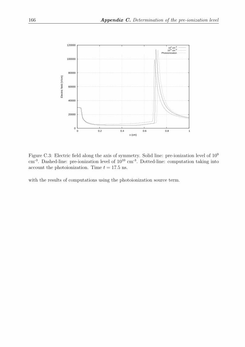
166 Appendix C. Determination of the pre-ionization level
0
20000
40000
60000
80000
100000
120000
0 0.2 0.4 0.6 0.8 1
Ele
ctric
fiel
d (V
/cm
)
x (cm)
109 cm-3
1010 cm-3
Photoionization
Figure C.3: Electric field along the axis of symmetry. Solid line: pre-ionization level of 109
cm-3. Dashed-line: pre-ionization level of 1010 cm-3. Dotted-line: computation taking intoaccount the photoionization. Time t = 17.5 ns.
with the results of computations using the photoionization source term.
Bibliography
Aints, M., A. Haljaste, T. Plank, and L. Roots (2008), Absorption of photo-ionizing ra-diation of corona discharges in air, Plasma Process. and Polym., 5 (7), 672–680, doi:10.1002/ppap.200800031.
Akishev, Y., I. Kochetov, A. Loboiko, and A. Napartovich (2002), 3-dimensional modelfor trichel pulses: results of numerical studies for air, in Proc. 8th Int. Symp. on HighPressure Low Temperature Plasma Chemistry (Puhajarve, Estonia), pp. 1–5.
Aleksandrov, N. L., and I. V. Kochetov (1996), Electron rate coefficients in gases undernon-uniform field and electron density conditions, J. Phys. D: Applied Physics, 29 (6),1476–1483.
Allegraud, K., O. Guaitella, and A. Rousseau (2007), Spatio-temporal breakdown in surfaceDBDs: evidence of collective effect, J. Phys. D: Applied Physics, 40 (24), 7698–7706.
Amestoy, P. R., I. S. Duff, and J.-Y. L’Excellent (2000), Multifrontal parallel distributedsymmetricand unsymmetric solvers, Comput. Methods Appl. Mech. Eng., 184, 501–520.
Amestoy, P. R., I. S. Duff, J. Koster, and J.-Y. L’Excellent (2001), A fully asynchronousmultifrontal solver using distributed dynamic scheduling, SIAM J. Matrix Anal. Appl.,23 (1), 15–41.
Amestoy, P. R., A. Guermouche, J.-Y. L’Excellent, and S. Pralet (2006), Hybrid schedulingfor the parallel solution of linear systems, Parallel Computing, 32 (2), 136–156.
Arrayás, M., U. Ebert, and W. Hundsdorfer (2002), Spontaneous branching of anode-directed streamers between planar electrodes, Phys. Rev. Lett., 88, 174502(R), doi:10.1103/PhysRevLett.88.174502.
Babaeva, N. Y., and G. V. Naidis (1996), Two-dimensional modelling of positive streamerdynamics in non-uniform electric fields in air, J. Phys. D: Applied Physics, 29, 2423–2431,doi:10.1088/0022-3727/29/9/029.
Babaeva, N. Y., and G. V. Naidis (1997), Dynamics of positive and negative streamers inair in weak uniform electric fields, IEEE Trans. Plasma Sci., 25, 375–379.
Babaeva, N. Y., A. N. Bhoj, and M. J. Kushner (2006), Streamer dynamics in gases con-taining dust particles, Plasma Sources Sci. Technol., 15, 591–602.
Bazelyan, E., and Y. Raizer (1998), Spark discharge, CRC Press, ISBN: 978-0849328688.
Bertein, H. (1973), Charges on insulators generated by breakdown of gas, J. Phys. D:Applied Physics, 6 (16), 1910–1916.
168 Bibliography
Bessières, D. (2006), Modélisation des décharges électriques filamentaires, Ph.D. thesis,University of Pau et des Pays de l’Adour, France.
Bessières, D., J. Paillol, A. Bourdon, P. Ségur, and E. Marode (2007), A new one-dimensional moving mesh method applied to the simulation of streamer discharges, J.Phys. D: Applied Physics, 40 (21), 6559–6570.
Boeuf, J.-P., and L. Pitchford (1991), Pseudospark discharges via computer simulation,IEEE Trans. Plasma Sci., 19 (2), 286–296, doi:10.1109/27.106826.
Boris, J. P., and D. L. Book (1973), Flux-Corrected Transport. I. SHASTA, A Fluid Trans-port Algorithm That Works, J. Comput. Phys., 11, 38–69.
Boris, J. P., and D. L. Book (1976), Flux-Corrected Transport. III. Minimal-Error FCTAlgorithms, J. Comput. Phys., 20, 397–431.
Bourdon, A., V. P. Pasko, N. Y. Liu, S. Célestin, P. Ségur, and E. Marode (2007), Effi-cient models for photoionization produced by non-thermal gas discharges in air basedon radiative transfer and the Helmholtz equations, Plasma Sources Sci. Technol., 16 (3),656–678, doi:10.1088/0963-0252/16/3/026.
Braun, D., V. Gibalov, and G. Pietsch (1992), Two-dimensional modelling of the dielectricbarrier discharge in air, Plasma Sources Sci. Technol., 1 (3), 166–174.
Briels, T. M. P., J. Kos, E. M. van Veldhuizen, and U. Ebert (2006), Circuit dependenceof the diameter of pulsed positive streamers in air, J. Phys. D: Applied Physics, 39,5201–5210.
Capeillère, J., P. Ségur, A. Bourdon, S. Célestin, and S. Pancheshnyi (2008), The finitevolume method solution of the radiative transfer equation for photon transport in non-thermal gas discharges: application to the calculation of photoionization in streamer dis-charges, J. Phys. D: Applied Physics, 41, 234018, doi:10.1088/0022-3727/41/23/234018.
Carlson, B. C. (1977), Elliptic integrals of the first kind, SIAM J. Math. Anal., 8 (2), 231–242, doi:10.1137/0508016.
Celestin, S., K. Allegraud, G. Canes-Boussard, N. Leick, O. Guaitella, and A. Rousseau(2008a), Patterns of plasma filaments propagating on a dielectric surface, IEEE Trans.Plasma Sci., 36 (4), 1326–1327, doi:10.1109/TPS.2008.924519.
Celestin, S., G. Canes-Boussard, O. Guaitella, A. Bourdon, and A. Rousseau (2008b),Influence of the charges deposition on the spatio-temporal self-organization of streamersin a DBD, J. Phys. D: Applied Physics, 41 (20), 205214 (10pp), doi:10.1088/0022-3727/41/20/205214.
Chanrion, O., and T. Neubert (2008), A pic-mcc code for simulation of streamer propagationin air, J. Comput. Phys., 227 (15), 7222–7245, doi:10.1016/j.jcp.2008.04.016.
Chirokov, A., A. Gutsol, A. Fridman, K. D. Sieber, J. M. Grace, and K. S. Robinson (2004),Analysis of two-dimensional microdischarge distribution in dielectric-barrier discharges,Plasma Sources Sci. Technol., 13 (4), 623–635.
Bibliography 169
Demmel, J. W., S. C. Eisenstat, J. R. Gilbert, X. S. Li, and J. W. H. Liu (1999a), Asupernodal approach to sparse partial pivoting, SIAM J. Matrix Anal. Appl., 20 (3),720–755.
Demmel, J. W., J. R. Gilbert, and X. S. Li (1999b), An asynchronous parallel supernodalalgorithm for sparse gaussian elimination, SIAM J. Matrix Anal. Appl., 20 (4), 915–952.
Dessantes, P. (2000), Modélisation de décharges électriques de type streamer dans l’air àhaute pression sous géométrie fortement non uniforme, Ph.D. thesis, University of ParisXI, Orsay, France.
DeVore, C. R. (1998), An improved limiter for multidimensional flux-corrected transport,Naval Research Report, NRL/MR/6440–98-8330, 1–19.
Dhali, S. K., and P. F. Williams (1987), Two-dimensional studies of streamers in gases, J.Appl. Phys., 62, 4696–4707.
Djakov, A. F., Y. K. Bobrov, and Y. V. Yourguelenas (1998), Modeling of a positivestreamer in air in a non-uniform external field, in Physics and Technology of ElectricPower Transmission, vol. Book 1, edited by A. F. Djakov, pp. 161–200, MPEI Publishers,Moscow.
Djermoune, D., E. Marode, and P. Ségur (1995a), Two dimensional modelling of a streamerinduced discharge, in Proc. 22th Int. Conf. on Phenomena in Ionized Gases (Hoboken,USA), pp. 33–34.
Djermoune, D., S. Samson, E. Marode, and P. Ségur (1995b), A time resolved two di-mensional modelling of the electrical behaviour and the chemical yield of the streamerinduced discharge, in Proc. 11th Int. Conf. on Gas Discharges and Their Applications(Chuo University, Tokyo, Japan), pp. 484–487.
Ducasse, O., L. Papageorghiou, O. Eichwald, N. Spyrou, and M. Yousfi (2007), Criticalanalysis on two-dimensional point-to-plane streamer simulations using the finite elementand finite volume methods, IEEE Trans. Plasma Sci., 35 (5, Part 1), 1287–1300.
Durand, E. (1966a), Electrostatique I. Les distributions., vol. 1, Masson et Cie.
Durand, E. (1966b), Electrostatique II. Problèmes généraux. Conducteurs., vol. 2, Massonet Cie.
Durand, E. (1966c), Electrostatique III. Méthodes de Calcul. Diélectriques., vol. 3, Massonet Cie.
Dyakonov, M. I., and V. Y. Kachorovskii (1988), Theory of streamer discharge in semicon-ductors, Soviet Physics JETP, Engl. Transl, 67, 1049–1054.
Dyakonov, M. I., and V. Y. Kachorovskii (1989), Streamer discharge in a homogeneousfield, Soviet Physics JETP, Engl. Transl, 68, 1070–1074.
Eliasson, B., and U. Kogelschatz (1991a), Modeling and applications of silent dischargeplasmas, IEEE Trans. Plasma Sci., 19 (2), 309–323, doi:10.1109/27.106829.
170 Bibliography
Eliasson, B., and U. Kogelschatz (1991b), Nonequilibrium volume plasma chemical process-ing, IEEE Trans. Plasma Sci., 19 (6), 1063–1077, doi:10.1109/27.125031.
Eyring, C. F., S. S. MacKeown, and R. A. Millikan (1928), Fields Currents from Points,Phys. Rev., 31, 900–909.
Fedkiw, R. P., T. Aslam, B. Merriman, and S. Osher (1999), A Non-oscillatory EulerianApproach to Interfaces in Multimaterial Flows (the Ghost Fluid Method), J. Comput.Phys., 152, 457–492.
Ferziger, J., and M. Peric (2002), Computational Methods for Fluid Dynamics, 3rd ed.,Springer-Verlag, ISBN: 3-540-42074-6.
Fiala, A., L. C. Pitchford, and J. P. Boeuf (1994), Two-dimensional, hybrid model of low-pressure glow discharges, Phys. Rev. E, 49 (6), 5607–5622, doi:10.1103/PhysRevE.49.5607.
Franz, R. C., R. J. Nemzek, and J. R. Winckler (1990), Television image of a large upwardelectric discharge above a thunderstorm system, Science, 249, 48.
Georghiou, G. E., R. Morrow, and A. C. Metaxas (1999), The theory of short-gap break-down of needle point-plane gaps in air using finite-difference and finite-element methods,J. Phys. D: Applied Physics, 32 (12), 1370–1385.
Gibalov, V. I., and G. J. Pietsch (2000), The development of dielectric barrier dischargesin gas gaps and on surfaces, J. Phys. D: Applied Physics, 33 (20), 2618–2636.
Gibou, F., R. P. Fedkiw, L.-T. Cheng, and M. Kang (2002), A Second-Order-AccurateSymmetric Discretization of the Poisson Equation on Irregular Domains, J. Comput.Phys., 176, 205–227.
Godunov, S. (1959), A finite difference method for the numerical computation and dis-continuous solutions of the equations of fluid dynamics, Matematicheskii Sbornik, 47,271–306, (in Russian) Translated US Joint Publ. Res. Service, JPRS 7226 (1969).
Golubovskii, Y. B., V. A. Maiorov, J. Behnke, and J. F. Behnke (2002), Influence ofinteraction between charged particles and dielectric surface over a homogeneous barrierdischarge in nitrogen, J. Phys. D: Applied Physics, 35 (8), 751–761.
Guaitella, O., F. Thevenet, C. Guillard, and A. Rousseau (2006), Dynamic of the plasmacurrent amplitude in a barrier discharge: influence of photocatalytic material, J. Phys.D: Applied Physics, 39 (14), 2964–2972.
Guikema, J., N. Miller, J. Niehof, M. Klein, and M. Walhout (2000), Spontaneous patternformation in an effectively one-dimensional dielectric-barrier discharge system, Phys. Rev.Lett., 85 (18), 3817–3820, doi:10.1103/PhysRevLett.85.3817.
Guo, J.-M., and C.-H. J. Wu (1993), Two-dimensional nonequilibrium fluid models forstreamers, IEEE Trans. Plasma Sci., 21 (6), 684–695, doi:10.1109/27.256788.
Hallac, A., G. E. Georghiou, and A. C. Metaxas (2003), Secondary emission effects onstreamer branching in transient non-uniform short-gap discharges, J. Phys. D: AppliedPhysics, 36, 2498–2509, doi:10.1088/0022-3727/36/20/011.
Bibliography 171
Harrington, R. F. (2001), Time-harmonic electromagnetic fields, IEEE Press, John Wileyand Sons, Inc., New York.
Hassouni, K., F. Massines, and J.-M. Pouvesle (2004), Plasmas Froids. Génération, carac-térisation et technologies, chap. Plasmas hors-équilibre à des pressions atmosphériques,pp. 49–108, Publications de l’Université de Saint-Etienne, ISBN: 2-86272-339-8.
Hong, J.-M., T. Shinar, M. Kang, and R. Fedkiw (2007), On boundary condition capturingfor multiphase interfaces, J. Sci. Comput., 31 (1-2), 99–125.
Kang, M., R. P. Fedkiw, and X. dong Liu (2000), A boundary condition capturing methodfor multiphase incompressible flow, J. Sci. Comput., 15, 323–360.
Kim, Y., J. Park, and S. Hong (2004), Geometrical effects of the discharge system on thecorona discharge and chemically active species generated in wire-cylinder and wire-platereactors, Journal of the Korean Physical Society, 44 (6), 1458–1467.
Klein, M., N. Miller, and M. Walhout (2001), Time-resolved imaging of spatiotemporalpatterns in a one-dimensional dielectric-barrier discharge system, Phys. Rev. E, 64 (2),026,402, doi:10.1103/PhysRevE.64.026402.
Kogelschatz, U. (2002), Filamentary, patterned, and diffuse barrier discharges, IEEE Trans.Plasma Sci., 30 (4), 1400–1408, doi:10.1109/TPS.2002.804201.
Kogelschatz, U. (2004), Atmospheric-pressure plasma technology, Plasma Phys. Control.Fusion, 46 (12B), B63–B75.
Kozlov, K. V., H.-E. Wagner, R. Brandenburg, and P. Michel (2001), Spatio-temporallyresolved spectroscopic diagnostics of the barrier discharge in air at atmospheric pressure,J. Phys. D: Applied Physics, 34 (21), 3164–3176.
Kulikovsky, A. A. (1995a), A more accurate Scharfetter-Gummel algorithm of electrontransport for semiconductor and gas discharge simulation, J. Comput. Phys., 119, 149–155.
Kulikovsky, A. A. (1995b), Two-dimensional simulation of the positive streamer in N2
between parallel-plate electrodes, J. Phys. D: Applied Physics, 28 (12), 2483–2493.
Kulikovsky, A. A. (1997a), Production of chemically active species in the air by a singlepositive streamer in a nonuniform field, IEEE Trans. Plasma Sci., 25 (3), 439–446, doi:10.1109/27.597258.
Kulikovsky, A. A. (1997b), Positive streamer between parallel plate electrodes in atmo-spheric pressure air, J. Phys. D: Applied Physics, 30, 441–450.
Kulikovsky, A. A. (1998), Positive streamer in a weak field in air: A moving avalanche-to-streamer transition, Phys. Rev. E, 57, 7066–7074, doi:10.1103/PhysRevE.57.7066.
Kulikovsky, A. A. (2000a), The role of photoionization in positive streamer dynamics, J.Phys. D: Applied Physics, 33, 1514–1524.
172 Bibliography
Kulikovsky, A. A. (2000b), The role of the absorption length of photoionizing radiation instreamer dynamics in weak fields: a characteristic scale of ionization domain, J. Phys.D: Applied Physics, 33 (1), L5–L7.
Kulikovsky, A. A. (2001), The efficiency of radicals production by positive streamer in air:the role of laplacian field, IEEE Trans. Plasma Sci., 29 (2), 313–317, doi:10.1109/27.922740.
Kunhardt, E. E., and Y. Tzeng (1988), Development of an electron avalanche and itstransition into streamers, Phys. Rev. A, 38, 1410–1421.
Kunhardt, E. E., J. Wu, and B. Penetrante (1988), Nonequilibrium macroscopic de-scriptions of electrons in weakly ionized gases, Phys. Rev. A, 37, 1654–1662, doi:10.1103/PhysRevA.37.1654.
Landau, L. D., and E. M. Lifshitz (1971), The classical theory of fields, Course of theoreticalphysics - Pergamon International Library of Science, Technology, Engineering and SocialStudies, Oxford: Pergamon Press, 1971, 3rd rev. engl. edition.
Larsen, E. W., G. Thömmes, A. Klar, M. Seaïd, and T. Götz (2002), Simplified PN Ap-proximations to the Equations of Radiative Heat Transfer and Applications, J. Comput.Phys., 183, 652–675.
Leonard, B., A. Lock, and M. MacVean (1995), Extended Numerical Integration for Gen-uinely Multidimensional Advective Transport Insuring Conservation, vol. 9, 1–12 pp.,Pineridge Press.
Leonard, B. P. (1979), A stable and accurate convective modelling procedure based onquadratic upstream interpolation, Comput. Meth. Appl. Mech. Engrg., 19, 59–98.
Leonard, B. P. (1991), The ULTIMATE conservative difference scheme applied to unsteadyone-dimensional advection, Comput. Methods Appl. Mech. Eng., 88, 17–74.
Li, C., W. J. M. Brok, U. Ebert, and J. J. A. M. van der Mullen (2007), Deviations fromthe local field approximation in negative streamer heads, J. Phys. D: Applied Physics,101 (12), 123305, doi:10.1063/1.2748673.
Liu, N. (2006), Dynamics of positive and negative streamers in sprites, Ph.D. thesis, ThePennsylvania State University, USA.
Liu, N., S. Célestin, A. Bourdon, V. P. Pasko, P. Ségur, and E. Marode (2007), Applicationof photoionization models based on radiative transfer and the Helmholtz equations tostudies of streamers in weak electric fields, Appl. Phys. Lett., 91 (21), 211501, doi:10.1063/1.2816906.
Liu, N. Y., and V. P. Pasko (2004), Effects of photoionization on propagation and branchingof positive and negative streamers in sprites, J. Geophys. Res., 109, A04301, doi:10.1029/2003JA010064.
Liu, N. Y., and V. P. Pasko (2006), Effects of photoionization on similarity propertiesof streamers at various pressures in air, J. Phys. D: Applied Physics, 39, 327–334, doi:10.1088/0022-3727/39/2/013.
Bibliography 173
Liu, X.-D., R. P. Fedkiw, and M. Kang (2000), A Boundary Condition Capturing Methodfor Poisson’s Equation on Irregular Domains, J. Comput. Phys., 160, 151–178.
Loeb, L. B. (1965), Ionizing Waves of Potential Gradient, Science, 148, 1417–1426.
Loeb, L. B., and J. M. Meek (1940a), The Mechanism of Spark Discharge in Air at Atmo-spheric Pressure. I, J. Appl. Phys., 11, 438–447.
Loeb, L. B., and J. M. Meek (1940b), The Mechanism of Spark Discharge in Air at Atmo-spheric Pressure. II, J. Appl. Phys., 11, 459–474.
Luque, A., U. Ebert, C. Montijn, and W. Hundsdorfer (2007), Photoionization in negativestreamers: Fast computations and two propagation modes, Appl. Phys. Lett., 90, 081501,doi:10.1063/1.2435934.
Lyons, W. A. (2006), The meteorology of transient luminous events - An introduction andoverview, in Sprites, Elves and Intense Lightning Discharges, NATO Science Series II:Mathematics, Physics and Chemistry, vol. 225, edited by M. Füllekrug and E. A. Mareevand M. J. Rycroft, pp. 19–56, Springer, Heidleberg, Germany.
Manley, T. C. (1943), The electric characteristics of the ozonator discharges, Trans. Elec-trochem. Soc., 84, 83–96.
Meek, J. M. (1940), A theory of spark discharge, Phys. Rev., 57 (8), 722–728, doi:10.1103/PhysRev.57.722.
Montijn, C., and U. Ebert (2006), Diffusion correction to the raether–meek criterionfor the avalanche-to-streamer transition, J. Phys. D: Applied Physics, 39 (14), 2979–2992.
Moreau, E. (2007), Airflow control by non-thermal plasma actuators, J. Phys. D: AppliedPhysics, 40 (3), 605–636.
Morrow, R. (1981), Numerical Solution of Hyperbolic Equations for Electron Drift inStrongly Non-Uniform Electric Fields, J. Comput. Phys., 43, 1–15.
Morrow, R., and J. J. Lowke (1997), Streamer propagation in air, J. Phys. D: AppliedPhysics, 30, 614–627.
Murooka, Y., T. Takada, and K. Hiddaka (2001), Nanosecond surface discharge and chargedensity evaluation, Part I: review and experiments, 17 (2), 6–16, doi:10.1109/57.917527.
Naidis, G. V. (1997), Effects of nonlocality on the dynamics of streamers in positive coronadischarges, Tech. Phys. Lett., 23, 493–494.
Naidis, G. V. (2006), On photoionization produced by discharges in air, Plasma SourcesSci. Technol., 15, 253–255.
Nguyen, D. Q., R. P. Fedkiw, and M. Kang (2001), A Boundary Condition CapturingMethod for Incompressible Flame Discontinuities, J. Comput. Phys., 172, 71–98.
Packan, D. (2003), Repetitive nanosecond glow discharge in atmospheric pressure air, Ph.D.thesis, Stanford University, USA.
174 Bibliography
Pai, D. (2008), Nanosecond repetitively pulsed plasmas in preheated air at atmsophericpressuregeneration of diffuse nonthermal plasmas in air at atmospheric pressure, Ph.D.thesis, Ecole Centrale Paris, France.
Pai, D., D. Lacoste, and C. Laux (2008), Images of nanosecond repetitively pulsed plasmasin preheated air at atmospheric pressure, IEEE Trans. Plasma Sci., 36 (4), 974–975,doi:10.1109/TPS.2008.924484.
Pancheshnyi, S. (2005), Role of electronegative gas admixtures in streamer start, propaga-tion and branching phenomena, Plasma Sources Sci. Technol., 14 (4), 645–653.
Pancheshnyi, S., M. Nudnova, and A. Starikovskii (2005), Development of a cathode-directed streamer discharge in air at different pressures: Experiment and comparisonwith direct numerical simulation, Phys. Rev. E, 71 (1), 016407, doi:10.1103/PhysRevE.71.016407.
Pancheshnyi, S. V., S. M. Starikovskaia, and A. Y. Starikovskii (2001), Role of photoioniza-tion processes in propagation of cathode-directed streamer, J. Phys. D: Applied Physics,34, 105–115.
Papageorghiou, L., and N. Spyrou (2007), Formation and propagation of ionization potentialwaves in various pressures, in Proc. 28th Int. Conf. on Phenomena in Ionized Gases(Prague, Czech Republic), pp. 1–4.
Parker, J. H., and J. J. Lowke (1969), Theory of electron diffusion parallel to electric fields.I. Theory, Phys. Rev., 181 (1), 290–301, doi:10.1103/PhysRev.181.290.
Pasko, V. P. (2006), NATO Science Series II: Mathematics, Physics and Chemistry Vol.225, chap. Theoretical modeling of sprites and jets, in Sprites, Elves and Intense LightningDischarges, pp. 253–293, Heidleberg: Springer.
Pasko, V. P. (2007), Red sprite discharges in the atmosphere at high altitude: the molecularphysics and the similarity with laboratory discharges, Plasma Sources Sci. Technol., 16,S13–S29, doi:10.1088/0963-0252/16/1/S02.
Pasko, V. P., U. S. Inan, and T. F. Bell (1998), Spatial structure of sprites, Geophys. Res.Lett., 25, 2123–2126.
Penney, G. W., and G. T. Hummert (1970), Photoionization measurements in Air, Oxygen,and Nitrogen, J. Appl. Phys., 41, 572–577.
Pilla, G., D. Galley, D. A. Lacoste, F. Lacas, D. Veynante, and C. O. Laux (2006), Sta-bilization of a turbulent premixed flame using a nanosecond repetitively pulsed plasma,IEEE Trans. Plasma Sci., 34 (6), 2471–2477, doi:10.1109/TPS.2006.886081.
Pomraning, G. (1973), The equations of radiation hydrodynamics, Pergamon Press, NewYork.
Potin, J. (2001), Modélisation numérique d’une décharge filamentaire controlée par bar-rière diélectrique dans l’azote à la pression atmosphérique, Ph.D. thesis, Université PaulSabatier de Toulouse, France.
Bibliography 175
Press, W. H., S. A. Teukolski, W. T. Vetterling, and B. P. Flannery (1992), NumericalRecipes in FORTRAN - The Art of Scientific Computing - Third Edition, UniversityPress, Cambridge.
Raizer, Y. P. (1991), Gas Discharge Physics, Springer-Verlag, New York, NY.
Rax, J.-M. (2005), Physique des Plasmas, Dunod, Paris.
Régnier, P. (2004), Modélisation de décharges filamentaires. Applications à la combustionet au traitement d’effluents gazeux, Ph.D. thesis, University of Rouen, France.
Scharfetter, D., and H. Gummel (1969), Large-signal analysis of a silicon read diode oscil-lator, IEEE Trans. Electron Devices, 16 (1), 64–77.
Ségur, P., A. Bourdon, E. Marode, D. Bessières, and J. H. Paillol (2006), The use of animproved Eddington approximation to facilitate the calculation of photoionization instreamer discharges, Plasma Sources Sci. Technol., 15, 648–660.
Sentman, D. D., E. M. Wescott, D. L. Osborne, D. L. Hampton, and M. J. Heavner (1995),Preliminary results from the Sprites94 campaign: Red sprites, Geophys. Res. Lett., 22,1205–1208.
Stanley, M., P. Krehbiel, M. Brook, C. Moore, W. Rison, and B. Abrahams (1999), Highspeed video of initial sprite development, Geophys. Res. Lett., 26, 3201–3204.
Starikovskaia, S. M. (2006), Plasma assisted ignition and combustion, J. Phys. D: AppliedPhysics, 39 (16), R265–R299.
Stone, H. L. (1968), Iterative solution of implicit approximations of multidimensional partialdifferential equations, SIAM J. Numer. Anal., 5 (3), 530–558.
Taine, J., and A. Soufiani (1999), Gas IR radiative properties: from spectroscopic data toapproximate models, in Advances in Heat Transfer, vol. 33, edited by J. Hartnett andT. Irvine, pp. 295–414, Academic Press, San Diego, California.
Teich, T. H. (1967), Emission gasionisierender strahlung aus electronenlawinen I. Meßanord-nung und Meßverfahren. Messungen in Sauerstoff, Z. Phys., 199, 378–394.
Tseng, Y.-H., and J. H. Ferziger (2003), A ghost-cell immersed boundary method for flowin complex geometry, J. Comput. Phys., 192 (2), 593–623.
Vitello, P. A., B. M. Penetrante, and J. N. Bardsley (1994), Simulation of negative-streamerdynamics in nitrogen, Phys. Rev. E, 49, 5574–5598.
Wu, C., and E. E. Kunhardt (1988), Formation and propagation of streamers in N2 andN2 − SF 6 mixtures, Phys. Rev. A, 37, 4396–4406.
Yurgelenas, Y. V., and H.-E. Wagner (2006), A computational model of a barrier dischargein air at atmospheric pressure: the role of residual surface charges in microdischargeformation, J. Phys. D: Applied Physics, 39 (18), 4031–4043.
Zalesak, S. T. (1979), Fully multidimensional flux-corrected transport algorithms for fluids,J. Comput. Phys., 31, 335–362.
176 Bibliography
Zalesak, S. T. (1979), Fully multidimensional flux-corrected transport algorithms for fluids,J. Comput. Phys., 31, 335–362.
Zeghondy, B., S. Célestin, A. Bourdon, P. Ségur, D. Bessières, and J. Paillol (2007), Animmersed boundary method to simulate positive streamer propagation in point-to-planegeometry in air, in Proc. 28th Int. Conf. on Phenomena in Ionized Gases (Prague, CzechRepublic), pp. 1–4.
Zheleznyak, M. B., A. K. Mnatsakanyan, and S. V. Sizykh (1982), Photoionization ofnitrogen and oxygen mixtures by radiation from a gas discharge, High Temp., 20, 357–362.
Zhu, Y., T. Takada, K. Sakai, and D. Tu (1996), The dynamic measurement of surfacecharge distribution deposited from partial discharge in air by pockels effect technique, J.Phys. D: Applied Physics, 29 (11), 2892–2900.