structure preserving optimal control of a 3d-dimensional ... · structure preserving optimal...
TRANSCRIPT
ECCOMAS Thematic Conference on Multibody DynamicsJune 29 - July 2, 2015, Barcelona, Catalonia, Spain
Structure preserving optimal control of a 3d-dimensional upright gait
Michael W. Koch∗, Sigrid Leyendecker#
∗ Institute of Applied MechanicsTechnische Universität Kaiserslautern
D-67653 Kaiserslautern, [email protected]
# Chair of Applied DynamicsUniversity of Erlangen-Nuremberg
D-91052 Erlangen, [email protected]
ABSTRACTThe optimal control of human locomotion requires simulation techniques, which handle the con-tact’s establishing and releasing between the foot and the ground. In this work, our aim is to op-timally control the human upright gait using a structure preserving variational integrator, wherebythe physiologically motivated cost functions of minimal kinetic energy is chosen and the obtainedresults are analysed with the gait of humans. Thereby, the three-dimensional rigid multibody sys-tem enables us to model forefoot as well as heel contact and its dynamics is simulated using astructure preserving method. The applied mechanical integrator is based on a discrete constrainedversion of the Lagrange-d’Alembert principle, which yields a symplectic momentum preservingmethod (see [13] for details). The investigated contact formulation covers the theory of perfectlyplastic contacts. To guarantee the structure preservation and the geometrical correctness, the non-smooth problem is solved including the contact configuration, time and force, in contrast to relyingon a smooth approximation of the contact problem via a penalty potential.
Keywords: structure preservation, perfectly plastic contact, bipedal upright gait, optimal control.
1 INTRODUCTIONThe human environment consists of a large variety of mechanical and biomechanical systems, inwhich different types of contact can occur. The biomechanical literature is often focussed on thefunction and structure of the human locomotor system in combination with the foot-ground con-tact, whereby cyclic walking movements come to the fore [7, 17]. Here, we are interested in theupright gait in conjunction with a structure preserving integrator. In contrast to movements withrolling wheels, the simulation of locomotion with legs requires the knowledge, how the contact’sestablishing and releasing between the feet and the ground works. The investigated contact for-mulation covers the theory of perfectly plastic contacts (e.g. see [10]), which means that the footstays in contact with the ground for a certain time.
The reduction to an armless bipedal walker represents the minimal multibody system to simulatehumanlike upright gait. The walker consists of an upper body representing the human torso andeach leg consists of three rigid bodies, which represent thigh, calf and the foot. The inclusion ofthe feet leads to movements that differ from those considered e.g. in [?]. The optimally controlledwalker allows actuation in the hip and the knee joints as well as in the two ankle joints, such that aphysiologically motivated cost function is minimised. In the numerical solution, a direct transcrip-tion method is used to transform the optimal control problem into an optimisation problem beingconstrained by the fulfilment of discrete equations of motion, boundary conditions and path con-straints, see e.g. [12, 21]. The walking motions are subdivided in two phases and they are calledsingle and double support phases. To avoid an artificial restriction of the optimisation problem’sphases by prescribing the time of contact establishing or releasing, variable time steps are used,wherefore the necessary scaling parameters are of the optimisation parameters.The straight posture of the homo sapiens’ gait is a characteristical attribute of the human species,whereby the evolution of the human gait results from an anthropological optimisation process.Initiated by climbing down from trees and leaving forests, the survival in velds necessitates aphysical adoption and the results are reflected by the kind of human locomotion respectively by
the physique: an upright gait shows benefits like a distinct all-round visibility, it reduces the waterloss as a consequence of evaporation and allows the possibility to use tools and weapons at thestruggle of survival. In paleoanthropology, the upright gait is appreciated as a key event of thehuman evolution with great changes of the anatomy: the human skeleton is optimised for bipedalwalking with the result of an efficient and economical locomotion.In biomechanical literature, the focus is often on analysing and simulating the upright gait withmuscle models, whereas in robotics the aim is to develop bipedal robotics with the humanlike ca-pability to move in various circumstances. In the area of computer graphics, a specific challengeis to create realistic movements for the virtual characters in video games or movies. According tothe different research interests, a large variety of models exists to analyse bipedal walking. Themodels in the field of biomechanics range from a simple spring mass system [9] – explaining thebasic dynamics of walking and running – to complex multibody systems with included musclesin [8]. These models are primarily used to investigate the acting forces within the body, but notto generate motions. In computer graphics, a lot of research is addressed to synthesise plausiblemotions and a further interesting point is, that in [19, 18] optimisation techniques find a transitionfrom a pre-recorded motion to another one.The aim of this paper is to compute physically valid and humanlike walking movements by us-ing the DMOCC approach, which means that the dynamics of the multibody system is discretisedby the variational integrator introduced in [13, 14] and the resulting equations of motion serve asequality constraints for the optimisation problem in which physiologically motivated cost functionof minimal kinetic energy is tested. In contrast to the forward respectively inverse dynamic sim-ulations, neither the trajectory nor the control sequence has to be exactly known for the walkingsystem, because an optimal trajectory and the corresponding actuation is determined by the op-timisation process subject to the evaluated objective function. Walking differs from running bythe feet’s contact sequence: walking is characterised by switching from single and double sup-port phases while running movements alternate between single support and flight phase. Often,in simpler models the double support phase is ignored, but herein it is an essential part of thefollowing motion sequence. Another aspect concerns the three different contact possibilities ofeach foot during the walking motion: namely, we have to differentiate between forefoot, heel anddouble contact. Finally, the optimisation of a humanlike bipedal walking requires the correct con-sideration of the single and double support phase and also the different contact scenarios for eachfoot.
Section 2 describes briefly the multibody formulation in redundant coordinates and introduces acorresponding actuation force formulation. The symplectic momentum integrator and the nullspace method with nodal reparametrisation, which reduces the numerical effort, are introducedin Section 3. Section 4 covers the optimal control problem and explains shortly the transfer intoa finite dimensional optimisation problem. The used bipedal walker model is described in Sec-tion 5 and the discrete equations of motion corresponding to the perfectly plastic contact for thevariational approach are given. In Section 6, the general human gait sequence is described and inSection 7, the discrete constrained optimisation problem is formulated. The result for the bipedalwalking with minimal kinetic energy is presented at the end of the paper.
2 RIGID MULTIBODY CONFIGURATION AND ACTUATIONIn this work, the rotation free formulation introduced in [3] for rigid bodies and in [5] for rigidmultibody systems is used to describe the configuration and to simulate the dynamics. The α-thrigid body is specified by a configuration vector qqqα(t)∈R12 composed by the placement of its cen-ter of mass ϕϕϕα(t) and the right-handed director triad dddα
i (t) for i = 1,2,3. The director triad speci-fies the body’s orientation in space and has to stay orthonormal during the motion in the consideredtime interval [t0, tN ], which is guaranteed by six so-called internal constraints gggint(qqq
α) = 000 ∈ R6.In multibody systems, the rigid bodies are interconnected by different types of joints, e.g. revoluteor spherical joints. The interconnection of the rigid bodies as well as their rigidity gives rise to a

scleronomic and holonomic constraint function ggg(qqq)∈Rm on the redundant configuration variableqqq ∈ Rk, where k equals 12 times the number of bodies. The multibody systems are actuated di-rectly by the independent generalised forces and torques τττ ∈Rk−m and the resulting k-dimensionalredundant actuation fff (qqq) ∈ Rk can be computed via fff (qqq) = BBBT (qqq) · τττ with the input transforma-tion matrix BBBT (qqq) ∈ Rk×(k−m). Note that the transformation matrix depends on the rigid bodies’interconnection and it is described in detail in [13].
3 STRUCTURE PRESERVING INTEGRATION FOR CONSTRAINED MECHANICALSYSTEMS
The dynamics of time-continuous mechanical systems can be described using the Lagrangian orHamiltonian formalism – in this work, the discrete Lagrangian mechanics is used to derive a struc-ture preserving integrator, see e.g. [16]. The constrained mechanical system is considered in aconfiguration manifold Q ⊆ Rk with the time-dependent configuration vector qqq(t) ∈ Q. Corre-sponding to the approach in [13], the constrained version of the Lagrange-d’Alembert principle isdiscretised at the time nodes {t0, t1 = t0 +∆t, . . . , tn = t0 + n∆t, . . . , tN = t0 +N∆t}, where N ∈ Nis the number of time intervals and the discrete configurations qqqn ≈ qqq(tn) approximate the con-tinuous trajectory. Similarly, λλλ n ≈ λλλ (tn) approximates the Lagrange multipliers λλλ (t) ∈ Rm. Asusual in the context of discrete variational mechanics, the discrete Lagrangian Ld : Q×Q→R isan approximation to the action integral of the continuous Lagrangian over one time-interval. Thediscrete Lagrange-d’Alembert principle requires stationarity of the resulting action sum, i.e.
δSd = δ
[N−1
∑n=0
Ld(qqqn,qqqn+1)−12(tn+1− tn)
[gggT (qqqn) ·λλλ n−gggT (qqqn+1) ·λλλ n+1
]]
+N−1
∑n=0
fff−n ·δqqqn + fff+n ·δqqqn+1 = 000
for all variations δqqqn with δqqq0 = δqqqN = 000and δλλλ n. This leads to the (k+m)-dimensional con-strained forced discrete Euler-Lagrange equations
D2Ld(qqqn−1, qqqn)+D1Ld(qqqn, qqqn+1)−GGGTd (qqqn) ·λλλ n + fff+n−1 + fff−n = 000 (1)
ggg(qqqn+1) = 000, (2)
for n = 1, . . . ,N − 1. Here GGGd = 12(tn+1− tn−1)
∂ggg(qqqn)
∂qqqdenotes the (m× k)-dimensional Jaco-
bian matrix of the constraints, and fff−n = 12(tn+1 − tn)BBBT (qqqn) · τττn, respectively fff+n−1 = 1
2(tn −tn−1)BBBT (qqqn) · τττn−1 are called left and right discrete forces. The resulting mechanical integra-tor represents exactly the behaviour of the analytical system concerning the consistency of themomentum maps and symplecticity. Due to these preservation properties it is called symplecticmomentum scheme. A further benefit of this mechanical integrator is the good energy behaviour,which means that there is no numerical gaining or dissipation of energy.According to [4, 5], we apply the discrete null space method to reduce the dimension of the con-strained forced discrete Euler-Lagrange equations. The discrete null space matrix PPP ∈ Rk×(k−m)
fulfils the property GGGd ·PPP = 000 and premultiplying Equation (1) by the transposed null space ma-trix, the constraint forces and thereby the Lagrange multipliers vanish. The resulting k-dimensionalsystem is called reduced forced discrete Euler-Lagrange equations. The minimal dimension of thesystem can be achieved using the vector of incremental generalised coordinates uuun+1 ∈U ⊂ R(k−m)
to reparametrise the configuration vector qqqn+1 in the neighbourhood of qqqn. The nodal reparametri-sation function FFFd : U×Q→ Q
qqqn+1 = FFFd(uuun+1,qqqn) (3)
fulfils the constraint conditions and therefore Equation (2) becomes unnecessary. Finally, thenumber of unknowns and thereby the numerical effort is reduced by the formulation in discrete
generalised coordinates uuud = {uuun}Nn=0 and the discrete torques τττd = {τττn}N−1
n=0 . The dimension ofthe equations of motion is reduced to k−m.
PPPT (qqqn) ·[D2Ld(qqqn−1,qqqn)+D1LLd(qqqn,FFFd(uuun+1,qqqn))+ fff+n−1(qqqn,τττn−1)+ fff−n (qqqn,τττn)
]= 000 (4)
4 OPTIMAL CONTROL PROBLEMIn general, the goal of optimal control problems is to determine the optimal state trajectory andforce field for a holonomically constrained system, which moves from the initial state qqq(t0) = qqq0,q̇qq(t0) = q̇qq0 to a final state qqq(tN) = qqqN , q̇qq(tN) = q̇qqN . The investigated system fulfils the equations ofmotion and at the same time the objective functional
J(qqq, q̇qq, fff ) =tN∫
t0
C(qqq, q̇qq, fff ) dt
is minimised, where the integrand C(qqq, q̇qq, fff ) : T Q×T ∗q Q→ R is a given cost function. The op-timal control problem is solved using a direct transcription method, which transforms it into aconstrained optimisation problem. The discrete objective function approximates the integral of thecontinuous cost function and the discrete constrained optimisation problems reads
minuuud ,τττd
J(uuud ,τττd) = minuuud ,τττd
N−1
∑n=0
C(uuun,uuun+1,τττn), (5)
subject to the constraints given by the reduced discrete equations of motion of the symplecticmomentum scheme in Equation (4). In addition to the discrete equations of motion of the spe-cific mechanical integrator, further constraints, like initial conditions, final conditions and possibleequality and inequality path constraints can be imposed.
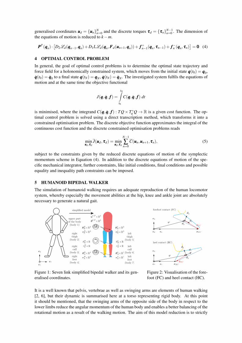
5 HUMANOID BIPEDAL WALKERThe simulation of humanoid walking requires an adequate reproduction of the human locomotorsystem, whereby especially the movement abilities at the hip, knee and ankle joint are absolutelynecessary to generate a natural gait.
Figure 1: Seven link simplified bipedal walker and its gen-eralised coordinates.
Figure 2: Visualisation of the fore-foot (FC) and heel contact (HC).
It is a well known that pelvis, vertebrae as well as swinging arms are elements of human walking[2, 6], but their dynamic is summarised here at a torso representing rigid body. At this pointit should be mentioned, that the swinging arms of the opposite side of the body in respect to thelower limbs reduce the angular momentum of the human body and enables a better balancing of therotational motion as a result of the walking motion. The aim of this model reduction is to strictly
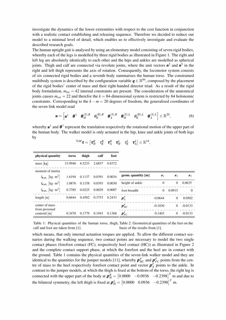
investigate the dynamics of the lower extremities with respect to the cost function in conjunctionwith a realistic contact establishing and releasing sequence. Therefore we decided to reduce ourmodel to a minimal level of detail, which enables us to effectively investigate and evaluate thedescribed research goals.The human upright gait is analysed by using an elementary model consisting of seven rigid bodies,whereby each of the legs is modelled by three rigid bodies as illustrated in Figure 1. The right andleft leg are absolutely identically to each other and the hips and ankles are modelled as sphericaljoints. Thigh and calf are connected via revolute joints, where the unit vectors nnn2 and nnn5 in theright and left thigh represents the axis of rotation. Consequently, the locomotor system consistsof six connected rigid bodies and a seventh body summarises the human torso. The constrainedmultibody system is described by the configuration variable qqq ∈ R84, composed by the placementof the rigid bodies’ center of mass and their right-handed director triad. As a result of the rigidbody formulation, mint = 42 internal constraints are present. The consideration of the anatomicaljoints causes mext = 22 and therefor the k = 84-dimensional system is restricted by 64 holonomicconstraints. Corresponding to the k−m = 20 degrees of freedom, the generalised coordinates ofthe seven link model read
uuu =[uuu1 θθθ
1θθθ(S),RH θ
(R),RK θθθ
(S),RA θθθ
(S),LH θ
(R),LK θθθ
(S),LA
]∈ R20, (6)
whereby uuu1 and θθθ1 represent the translation respectively the rotational motion of the upper part of
the human body. The walker model is only actuated in the hip, knee and ankle joints of both legsby
7LMτττ =
[τττR
H τRK τττR
A τττLH τL
K τττLA
]∈ R14,
physical quantity torso thigh calf foot
mass [kg] 33.9946 6.5233 2.6857 0.8372
moment of inertia
Ieee1eee1
[kg ·m2
]1.6194 0.1137 0.0391 0.0034
Ieee2eee2
[kg ·m2
]1.0876 0.1158 0.0393 0.0030
Ieee3eee3
[kg ·m2
]0.3785 0.0225 0.0029 0.0007
length [m] 0.6644 0.4582 0.3753 0.2433
center of massfrom proximalcentroid [m] 0.3470 0.1779 0.1943 0.1368
Table 1: Physical quantities of the human torso, thigh,calf and foot are taken from [1].
geom. quantity [m] eee1 eee2 eee3
height of ankle 0 0 0.0635
foot breadth 0 0.0915 0
ρρρFA -0.0644 0 0.0502
ρρρFHC -0.1030 0 -0.0133
ρρρFFC 0.1403 0 -0.0133
Table 2: Geometrical quantities of the feet on thebasis of the results from [1].
which means, that only internal actuation torques are applied. To allow the different contact sce-narios during the walking sequence, two contact points are necessary to model the two singlecontact phases (forefoot contact (FC), respectively heel contact (HC)) as illustrated in Figure 2and the complete contact support phase, at which the forefoot and the heel are in contact withthe ground. Table 1 contains the physical quantities of the seven-link walker model and they areidentical to the quantities for the jumper models [11], whereby ρρρF
HC and ρρρFFC points from the cen-
tre of mass to the heel respectively forefoot contact point and vector ρρρFA points to the ankle. In
contrast to the jumper models, at which the thigh is fixed at the bottom of the torso, the right leg isconnected with the upper part of the body at ρρρR
H =[0.0000 −0.0936 −0.2398
]T m and due to
the bilateral symmetry, the left thigh is fixed at ρρρLH =
[0.0000 0.0936 −0.2398
]T m.
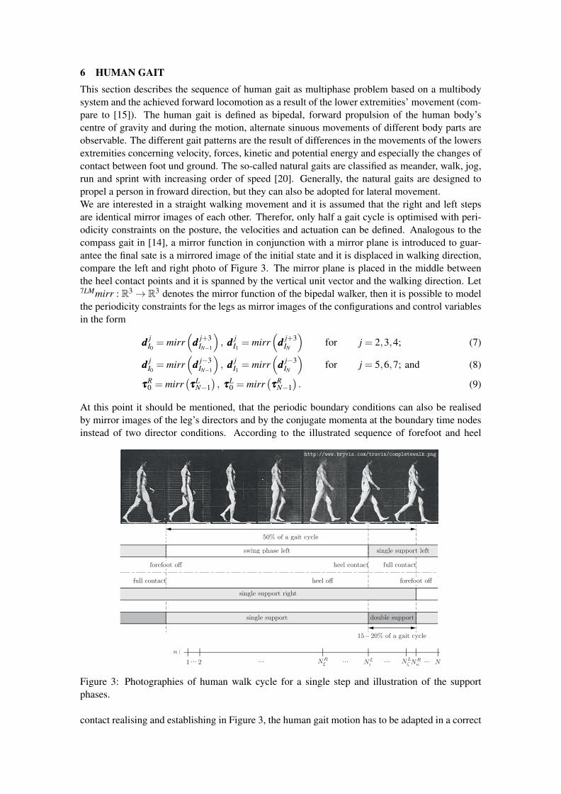
6 HUMAN GAITThis section describes the sequence of human gait as multiphase problem based on a multibodysystem and the achieved forward locomotion as a result of the lower extremities’ movement (com-pare to [15]). The human gait is defined as bipedal, forward propulsion of the human body’scentre of gravity and during the motion, alternate sinuous movements of different body parts areobservable. The different gait patterns are the result of differences in the movements of the lowersextremities concerning velocity, forces, kinetic and potential energy and especially the changes ofcontact between foot und ground. The so-called natural gaits are classified as meander, walk, jog,run and sprint with increasing order of speed [20]. Generally, the natural gaits are designed topropel a person in froward direction, but they can also be adopted for lateral movement.We are interested in a straight walking movement and it is assumed that the right and left stepsare identical mirror images of each other. Therefor, only half a gait cycle is optimised with peri-odicity constraints on the posture, the velocities and actuation can be defined. Analogous to thecompass gait in [14], a mirror function in conjunction with a mirror plane is introduced to guar-antee the final sate is a mirrored image of the initial state and it is displaced in walking direction,compare the left and right photo of Figure 3. The mirror plane is placed in the middle betweenthe heel contact points and it is spanned by the vertical unit vector and the walking direction. Let7LMmirr : R3→ R3 denotes the mirror function of the bipedal walker, then it is possible to modelthe periodicity constraints for the legs as mirror images of the configurations and control variablesin the form
ddd jI0= mirr
(ddd j+3
IN−1
), ddd j
I1= mirr
(ddd j+3
IN
)for j = 2,3,4; (7)
ddd jI0= mirr
(ddd j−3
IN−1
), ddd j
I1= mirr
(ddd j−3
IN
)for j = 5,6,7; and (8)
τττR0 = mirr
(τττ
LN−1), τττ
L0 = mirr
(τττ
RN−1). (9)
At this point it should be mentioned, that the periodic boundary conditions can also be realisedby mirror images of the leg’s directors and by the conjugate momenta at the boundary time nodesinstead of two director conditions. According to the illustrated sequence of forefoot and heel
Figure 3: Photographies of human walk cycle for a single step and illustration of the supportphases.
contact realising and establishing in Figure 3, the human gait motion has to be adapted in a correct
order in the continuous optimal control problem as well as in the discrete optimisation problem.In both cases, the double support phase represents the essential challenges of the human walkingphases. Comparing with running, the walking movement is characterised by the chronology ofsingle and double support phases and thus at every time at least one foot is in contact with theground: no flight phase occurs as observable e.g. in running motions.
7 OPTIMAL CONTROL OF THE BIPEDAL JUMPERThe constrained optimisation problem is formulated in terms of generalised coordinates 7LMuuudand the actuation torques 7LMτττd . In case of free motion (no contacts occur), the dynamical systemis restricted by the internal and external constraints in order to model the rigidity of the bodiesand the structural composition of the multibody system itself. The dynamic of the seven-linkmodel is described by a 20-dimensional system of equations. In all five walking sections, thesame relative nodal reparametrisation is used to update the configuration in dependence of thegeneralised coordinates. The equations of motion during the walking phases are premultipliedwith the appropriate forefoot respectively full contact discrete null space matrices to eliminate theconstraint forces including the contact forces. The equations of motion are premultiplied by thecorresponding null space matrix to achieve a reduced dimension of the equation of motions. Atthe end of the optimised walking phase, the left leg is in full contact with the ground. The contactsbetween the feet and the ground are modelled as perfectly plastic contact and the orientation of thecontact force prevents penetrating the ground. As a result of the different contact scenarios duringthe walking phases, the Lagrange multipliers are determined in post-processing via
λλλCn = RRRTΓ(qqqn) ·
[D2Ld(qqqn−1,qqqn)+D1Ld(qqqn,qqqn+1)+ fff+n−1 + fff−n
],
where
RRRΓ(qqqn) =7LMGGGT
Γ(qqqn) ·(7LMGGGΓ(qqqn) · 7LMGGGT
Γ(qqqn))−1
for Γ = FHC,HC,FC, (10)
which is formulated with the discrete Jacobian RRRΓ(qqqn) of the seven-link model. During the doublesupport phases, the Coulomb’s static friction law has to be fulfilled for the feet and consequentlytwo inequality constraints are necessary.The determination of the respective null space matrices for the double support phase is avoidedby taking a similar approach as for the transfer of contact at the compass gait. The first doublesupport phase is characterised by the forefoot contact of the right leg and by the heel contact of theleft leg. At first, the Euler-Lagrange equations are premultiplied by the transposed discrete nullspace matrix RPPPFC to eliminate the contact forces at the right foot, afterwards we premultiply thepartially reduced equations of motion again by the following projection matrix
QQQHC = III−(LGGGHC · RPPPFC
)T ·((LGGGHC · RPPPFC
)·(LGGGHC · RPPPFC
)T)−1· LGGGHC · RPPPFC ∈ R17×17.
At the second double support phase – forefoot contact on the right foot and full contact on the leftleg – the equations of motion are premultiplied at first by LPPPT
FC and then by the matrix
QQQHFC = III−(RGGGHFC · LPPPHC
)T ·((RGGGHFC · LPPPHC
)·(RGGGHFC · LPPPHC
)T)−1·LGGGHFC ·RPPPFC ∈R17×17.
Due to the unknown switching times between the different walking sequences, four scaling pa-rameters summarised in σσσ =
[σ1 σ2 σ3 σ4
]T ∈ R4 are required and they are also part of theoptimisation variables. It is necessary to mention, that the scaling parameter σ1 is used twice,namely at the single support phases at the beginning and at the end of the optimisation problem.This parameters enables the optimiser to shorten or extend each walking phase inside the scalinglimits. Finally, the discrete constrained optimisation problem of the half cycle gait for the chosenconditions reads
minuuud ,τττd ,σσσ
J(uuud ,τττd ,σσσ) =N−1
∑n=1
C(uuun,uuun+1,τττn,τττn+1, tn, tn+1)
subject to
◦ reduced forced discrete equations of motion of the single support phase with full contact in[t0, tξ
]for the right foot (α = R) and in [tκ , tN ] for the left foot (α = L)
αPPPTFHC(qqqn) ·
[D2Ld(qqqn−1,qqqn)+D1Ld(qqqn,qqqn+1)+ fff+n−1 + fff−n
]= 000
αgggFHC(qqqn+1) = 000
◦ constrained motion of the single support phase with forefoot contact in]tξ , tι
[for the right
foot
RPPPTFC(qqqn) ·
[D2Ld(qqqn−1,qqqn)+D1Ld(qqqn,qqqn+1)+ fff+n−1 + fff−n
]= 000
RgggFC(qqqn+1) = 000
◦ constrained motion of the double support phase with forefoot contact of the right foot andheel contact of the left foot in
[tι , tζ
]LQQQHC · RPPPT
FC(qqqn) ·[D2Ld(qqqn−1,qqqn)+D1Ld(qqqn,qqqn+1)+ fff+n−1 + fff−n
]= 000
RgggFC(qqqn+1) = 000LgggHC(qqqn+1) = 000
◦ constrained motion of the double support phase forefoot contact of the right foot and fullcontact at the left leg in
]tζ , tκ
[RQQQFC · LPPPT
FHC(qqqn) ·[D2Ld(qqqn−1,qqqn)+D1Ld(qqqn,qqqn+1)+ fff+n−1 + fff−n
]= 000
RgggFC(qqqn+1) = 000LgggFHC(qqqn+1) = 000
◦ periodic boundary conditions of equation (7) – (9) are summarised by
7LMbbb(qqq0,qqq1,qqqN−1,qqqN ,τττ1,τττN−1) = 000 (11)
◦ path constraints for n = 1, . . . ,N
7LMhhheq(qqqn) = 000 7LMhhhineq(qqqn)< 000
◦ path constraints single support
� full contact for n = 1, . . . ,Nξ −1 and n = Nκ +1, . . . ,N−1
right leg: n = 1, . . . ,Nξ −1:
√(λ 1
FHC,n
)2+(
λ 2FHC,n
)2−µ0‖λ 3
FHC,n +λ 6FHC,n‖< 0
right leg: n = Nξ : λ 4FHC,n = λ 5
FHC,n = λ 6FHC,n = 0
left leg: n = Nκ +1, . . . ,N−1:
√(λ 1
FHC,n
)2+(
λ 2FHC,n
)2−µ0‖λ 3
FHC,n +λ 6FHC,n‖< 0
� forefoot contact for n = Nζ +1, . . . ,Nι −1
right leg:
√(λ 1
FC,n
)2+(
λ 2FC,n
)2−µ0‖λ 3
FC,n‖< 0
◦ path constraints double support
� single/single contact for n = Nι , . . . ,Nζ −1
left foot:
√(λ 1
HC,n
)2+(
λ 2HC,n
)2−µ0‖λ 3
HC,n‖< 0
right foot:
√(λ 1
FC,n
)2+(
λ 2FC,n
)2−µ0‖λ 3
FC,n‖< 0
� single/full contact for n = Nζ , . . . ,Nκ
left leg: n = Nζ , . . .Nκ :
√(λ 1
FHC,n
)2+(
λ 2FHC,n
)2−µ0‖λ 3
FHC,n +λ 6FHC,n‖< 0
right leg: for n = Nζ , . . .Nκ−1:
√(λ 1
FC,n
)2+(
λ 2FC,n
)2−µ0‖λ 3
FC,n‖< 0
right n = Nκ : λ 1FC,n = λ 2
FC,n = λ 3FC,n = 0
◦ scaling paramerters
σσσLB ≤ σσσ ≤ σσσUB.
Each of the walking phases is scaled by its appropriate scaling parameter; remind that σ1 is usedtwice, namely at the single support phases at the beginning and at the end. Analogous to theoptimisation of the jumping movement in [11], the scaling parameters yield a lower and upperbound of the manoeuvre time for the half gait, while the optimiser manoeuvre time is determinedby the optimiser.
7.1 Minimal kinetic energy per step length
3
-0.4
-0.2
0
0.2
0.4
0.6
0.8
1
1.2
1.4
1.6
1
-0.5 -0.25 0 0.25 0.5 0.75 1 1.25 1.5 1.75 2 2.25 2.5 2.75 3 3.25 3.5 3.75 4 4.25 4.5 4.75 5 5.25 5.5
≈ 2 x 0.6338
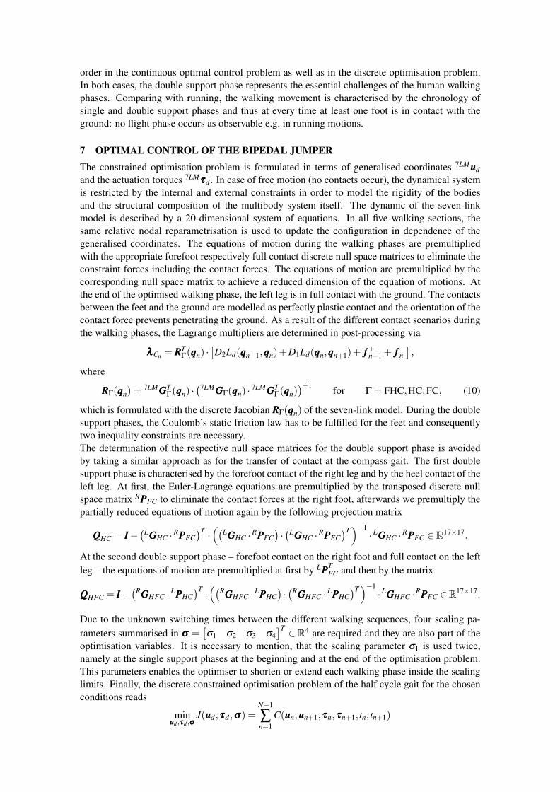
Figure 4: Minimal kinetic energy per step length: snapshots of the optimised bipedal motion.
The optimised motion for the criterion of Minimal kinetic energy per step length is presented in thefollowing lines. In Figure 4, the trajectories of the human and the feet as well as some characteris-tical snapshots are given. Obviously, as the trajectory of the swinging leg indicates, the foot is onlylifted up as little as possible – the feet’s center of mass is always below a height of 0.2 m (compareto Figure 4). The kinetic energy sum for a step-length of about 0.6338 m is computed to 41.2256 Js. The optimiser extends all walking phases according to σσσ =
[1.5000 1.5000 1.4889 1.4724
],
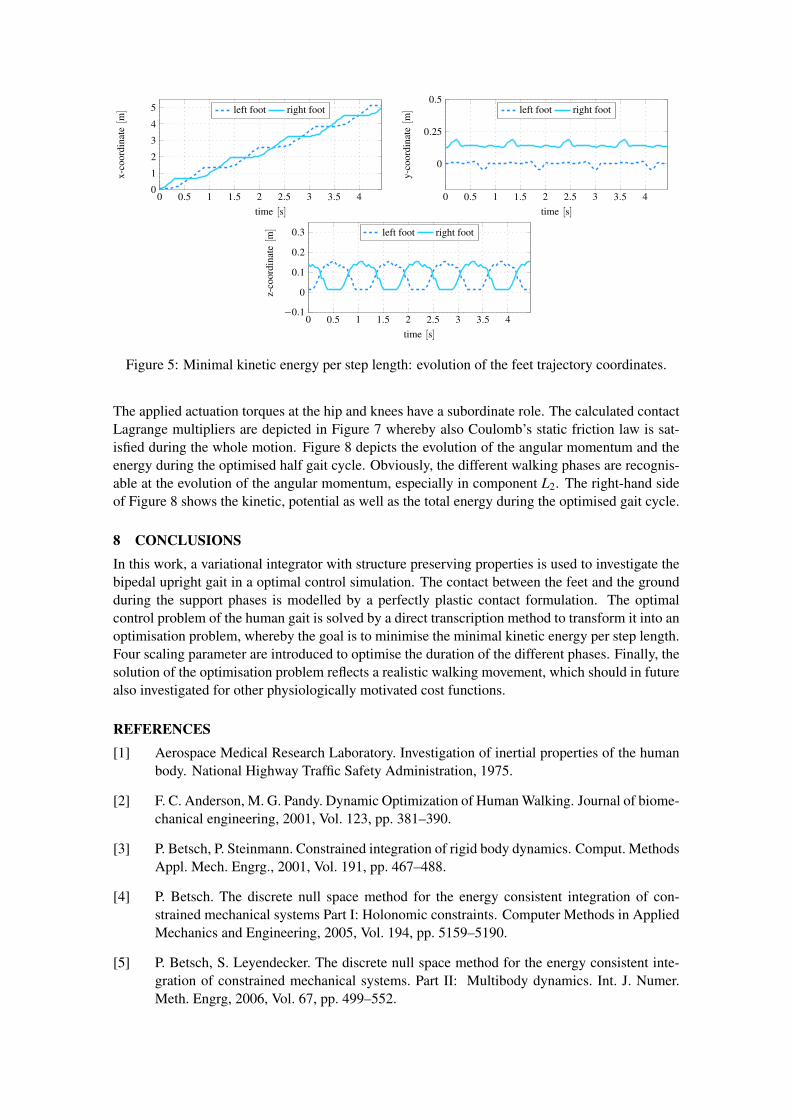
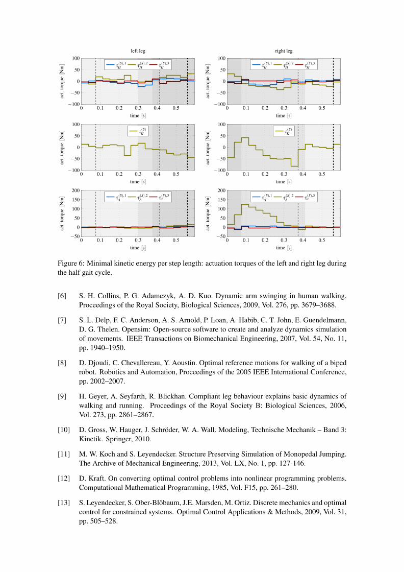
which is in all four cases exactly or almost the maximum scaling parameters and the walking mo-tion takes 0.5988 s. Another interpretation of this cost-function is, that we are interested at theminimal velocity per step-length, because the kinetic energy is directly proportional to the walk-ing speed. The feet’s trajectory over time is illustrated in Figure 5 and obviously, the comparativelylarge rotational motions at the angle joint can be observed. This can be explained by the fact thatdue to the small mass of the feet the resulting energy is small. Obviously, the standing leg is pri-marily actuated in eee2-direction at the angle joint during the forefoot contact, compare to Figure 6.
0 0.5 1 1.5 2 2.5 3 3.5 40
1
2
3
4
5
time [s]
x-co
ordi
nate
[m] left foot right foot
0 0.5 1 1.5 2 2.5 3 3.5 4
0
0.25
0.5
time [s]
y-co
ordi
nate
[m] left foot right foot
0 0.5 1 1.5 2 2.5 3 3.5 4−0.1
0
0.1
0.2
0.3
time [s]
z-co
ordi
nate
[m] left foot right foot
Figure 5: Minimal kinetic energy per step length: evolution of the feet trajectory coordinates.
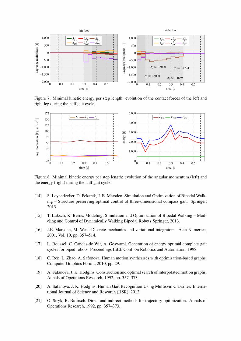
The applied actuation torques at the hip and knees have a subordinate role. The calculated contactLagrange multipliers are depicted in Figure 7 whereby also Coulomb’s static friction law is sat-isfied during the whole motion. Figure 8 depicts the evolution of the angular momentum and theenergy during the optimised half gait cycle. Obviously, the different walking phases are recognis-able at the evolution of the angular momentum, especially in component L2. The right-hand sideof Figure 8 shows the kinetic, potential as well as the total energy during the optimised gait cycle.
8 CONCLUSIONSIn this work, a variational integrator with structure preserving properties is used to investigate thebipedal upright gait in a optimal control simulation. The contact between the feet and the groundduring the support phases is modelled by a perfectly plastic contact formulation. The optimalcontrol problem of the human gait is solved by a direct transcription method to transform it into anoptimisation problem, whereby the goal is to minimise the minimal kinetic energy per step length.Four scaling parameter are introduced to optimise the duration of the different phases. Finally, thesolution of the optimisation problem reflects a realistic walking movement, which should in futurealso investigated for other physiologically motivated cost functions.
REFERENCES[1] Aerospace Medical Research Laboratory. Investigation of inertial properties of the human
body. National Highway Traffic Safety Administration, 1975.
[2] F. C. Anderson, M. G. Pandy. Dynamic Optimization of Human Walking. Journal of biome-chanical engineering, 2001, Vol. 123, pp. 381–390.
[3] P. Betsch, P. Steinmann. Constrained integration of rigid body dynamics. Comput. MethodsAppl. Mech. Engrg., 2001, Vol. 191, pp. 467–488.
[4] P. Betsch. The discrete null space method for the energy consistent integration of con-strained mechanical systems Part I: Holonomic constraints. Computer Methods in AppliedMechanics and Engineering, 2005, Vol. 194, pp. 5159–5190.
[5] P. Betsch, S. Leyendecker. The discrete null space method for the energy consistent inte-gration of constrained mechanical systems. Part II: Multibody dynamics. Int. J. Numer.Meth. Engrg, 2006, Vol. 67, pp. 499–552.
0 0.1 0.2 0.3 0.4 0.5−100
−50
0
50
100
time [s]
act.
torq
ue[N
m]
left leg
τ(S),1H τ
(S),2H τ
(S),3H
0 0.1 0.2 0.3 0.4 0.5−100
−50
0
50
100
time [s]
act.
torq
ue[N
m] τ
(S)K
0 0.1 0.2 0.3 0.4 0.5−50
0
50
100
150
200
time [s]
act.
torq
ue[N
m] τ
(S),1A τ
(S),2A τ
(S),3a
0 0.1 0.2 0.3 0.4 0.5−100
−50
0
50
100
time [s]
act.
torq
ue[N
m]
right leg
τ(S),1H τ
(S),2H τ
(S),3H
0 0.1 0.2 0.3 0.4 0.5−100
−50
0
50
100
time [s]
act.
torq
ue[N
m] τ
(S)K
0 0.1 0.2 0.3 0.4 0.5−50
0
50
100
150
200
time [s]
act.
torq
ue[N
m] τ
(S),1A τ
(S),2A τ
(S),3a
Figure 6: Minimal kinetic energy per step length: actuation torques of the left and right leg duringthe half gait cycle.
[6] S. H. Collins, P. G. Adamczyk, A. D. Kuo. Dynamic arm swinging in human walking.Proceedings of the Royal Society, Biological Sciences, 2009, Vol. 276, pp. 3679–3688.
[7] S. L. Delp, F. C. Anderson, A. S. Arnold, P. Loan, A. Habib, C. T. John, E. Guendelmann,D. G. Thelen. Opensim: Open-source software to create and analyze dynamics simulationof movements. IEEE Transactions on Biomechanical Engineering, 2007, Vol. 54, No. 11,pp. 1940–1950.
[8] D. Djoudi, C. Chevallereau, Y. Aoustin. Optimal reference motions for walking of a bipedrobot. Robotics and Automation, Proceedings of the 2005 IEEE International Conference,pp. 2002–2007.
[9] H. Geyer, A. Seyfarth, R. Blickhan. Compliant leg behaviour explains basic dynamics ofwalking and running. Proceedings of the Royal Society B: Biological Sciences, 2006,Vol. 273, pp. 2861–2867.
[10] D. Gross, W. Hauger, J. Schröder, W. A. Wall. Modeling, Technische Mechanik – Band 3:Kinetik. Springer, 2010.
[11] M. W. Koch and S. Leyendecker. Structure Preserving Simulation of Monopedal Jumping.The Archive of Mechanical Engineering, 2013, Vol. LX, No. 1, pp. 127-146.
[12] D. Kraft. On converting optimal control problems into nonlinear programming problems.Computational Mathematical Programming, 1985, Vol. F15, pp. 261–280.
[13] S. Leyendecker, S. Ober-Blöbaum, J.E. Marsden, M. Ortiz. Discrete mechanics and optimalcontrol for constrained systems. Optimal Control Applications & Methods, 2009, Vol. 31,pp. 505–528.
0 0.1 0.2 0.3 0.4 0.5−2,000
−1,500
−1,000
−500
0
500
1,000
time [s]
Lag
rang
em
ultip
liers
[1]
left foot
λ 1FC λ 2
FC λ 3FC
λ 1HC λ 2
HC λ 3HC
0 0.1 0.2 0.3 0.4 0.5−2,000
−1,500
−1,000
−500
0
500
1,000
σ1 ≈ 1.5000
σ2 ≈ 1.5000
σ3 ≈ 1.4889
σ4 ≈ 1.4724
time [s]
Lag
rang
em
ultip
liers
[1]
right foot
λ 1FC λ 2
FC λ 3FC
λ 1HC λ 2
HC λ 3HC
Figure 7: Minimal kinetic energy per step length: evolution of the contact forces of the left andright leg during the half gait cycle.
0 0.1 0.2 0.3 0.4 0.5−25
0
25
50
75
100
125
150
175
time [s]
ang.
mom
entu
m[ kg·m
2·s−
2] L1 L2 L3
0 0.1 0.2 0.3 0.4 0.50
1,000
2,000
3,000
4,000
5,000
time [s]
ener
gy[J]
EKin EPot ETot
Figure 8: Minimal kinetic energy per step length: evolution of the angular momentum (left) andthe energy (right) during the half gait cycle.
[14] S. Leyendecker, D. Pekarek, J. E. Marsden. Simulation and Optimization of Bipedal Walk-ing – Structure preserving optimal control of three-dimensional compass gait. Springer,2013.
[15] T. Luksch, K. Berns. Modeling, Simulation and Optimization of Bipedal Walking – Mod-eling and Control of Dynamically Walking Bipedal Robots Springer, 2013.
[16] J.E. Marsden, M. West. Discrete mechanics and variational integrators. Acta Numerica,2001, Vol. 10, pp. 357–514.
[17] L. Roussel, C. Candas-de Wit, A. Goswami. Generation of energy optimal complete gaitcycles for biped robots. Proceedings IEEE Conf. on Robotics and Automation, 1998.
[18] C. Ren, L. Zhao, A. Safonova. Human motion synthesises with optimisation-based graphs.Computer Graphics Forum, 2010, pp. 29.
[19] A. Safanova, J. K. Hodgins. Construction and optimal search of interpolated motion graphs.Annals of Operations Research, 1992, pp. 357–373.
[20] A. Safanova, J. K. Hodgins. Human Gait Recognition Using Multisvm Classifier. Interna-tional Journal of Science and Research (IJSR), 2012.
[21] O. Stryk, R. Bulirsch. Direct and indirect methods for trajectory optimization. Annals ofOperations Research, 1992, pp. 357–373.