structural dynamics final year - structural engineering bsc

STRUCTURAL DYNAMICS

Final Year - Structural Engineering BSc(Eng)

Structural Dynamics

D.I.T. Bolton St ii C. Caprani

Contents

1. Introduction to Structural Dynamics 1 2. Single Degree-of-Freedom Systems 8

a. Fundamental Equation of Motion

b. Free Vibration of Undamped Structures c. Free Vibration of Damped Structures

d. Forced Response of an SDOF System

3. Multi-Degree-of-Freedom Systems 20

a. General Case (based on 2DOF) b. Free-Undamped Vibration of 2DOF Systems

4. Continuous Structures 28

a. Exact Analysis for Beams

b. Approximate Analysis – Bolton’s Method

5. Practical Design 42

a. Human Response to Dynamic Excitation b. Crowd/Pedestrian Dynamic Loading

c. Damping in Structures d. Rules of Thumb for Design

6. Appendix 54

a. References

b. Important Formulae c. Important Tables and Figures

Structural Dynamics

D.I.T. Bolton St 1 C. Caprani

1. Introduction to Structural Dynamics Modern structures are increasingly slender and have reduced redundant strength

due to improved analysis and design methods. Such structures are increasingly

responsive to the manner in which loading is applied with respect to time and hence

the dynamic behaviour of such structures must be allowed for in design; as well as

the usual static considerations. In this context then, the word dynamic simply means

“changes with time”; be it force, deflection or any other form of load effect.

Examples of dynamics in structures are:

- Soldiers breaking step as they cross a bridge to prevent harmonic excitation;

- The Tacoma Narrows Bridge footage, failure caused by vortex shedding;

- the London Millennium Footbridge: lateral synchronise excitation.

(a)

(b)

Figure 1.1

The most basic dynamic system is the mass-spring system. An example is shown in

Figure 1.1(a) along with the structural idealisation of it in Figure 1.1(b). This is known

as a Single Degree-of-Freedom (SDOF) system as there is only one possible

displacement: that of the mass in the vertical direction. SDOF systems are of great

m

k

Structural Dynamics


importance as they are relatively easily analysed mathematically, are easy to

understand intuitively, and structures usually dealt with by Structural Engineers can

be modelled approximately using an SDOF model (see Figure 1.2 for example).

Figure 1.2

If we consider a spring-mass system as shown in Figure 1.3 with the properties m =

10 kg and k = 100 N/m and if give the mass a deflection of 20 mm and then release

it (i.e. set it in motion) we would observe the system oscillating as shown in Figure

1.3. From this figure we can identify that the time between the masses recurrence at

a particular location is called the period of motion or oscillation or just the period, and

we denote it T; it is the time taken for a single oscillation. The number of oscillations

per second is called the frequency, denoted f, and is measured in Hertz (cycles per

second). Thus we can say:

1fT

= (1.1)

We will show (Section 2.b, equation (2.19)) for a spring-mass system that:

12

kfmπ

= (1.2)

Structural Dynamics


In our system:

1 100 0.503 Hz2 10

fπ

= =

And from equation (1.1):

1 1 1.987 secs0.503

Tf

= = =

We can see from Figure 1.3 that this is indeed the period observed.

-25

-20

-15

-10

-5

0

5

10

15

20

25

0 0.5 1 1.5 2 2.5 3 3.5 4

Time (s)

Dis

plac

emen

t(m

m)

Period T

Figure 1.3

To reach the deflection of 20 mm just applied, we had to apply a force of 2 N, given

that the spring stiffness is 100 N/m. As noted previously, the rate at which this load is

applied will have an effect of the dynamics of the system. Would you expect the

system to behave the same in the following cases?

- If a 2 N weight was dropped onto the mass from a very small height?

- If 2 N of sand was slowly added to a weightless bucket attached to the mass?

Assuming a linear increase of load, to the full 2 N load, over periods of 1, 3, 5 and 10

seconds, the deflections of the system are shown in Figure 1.4.

m = 10 kg

k = 100 N/m

Structural Dynamics


Dynamic Effect of Load Application Duration

0

5

10

15

20

25

30

35

40

0 2 4 6 8 10 12 14 16 18 20

Time (s)

Def

lect

ion

(mm

)

1-sec

3-sec

5-sec

10-sec

Figure 1.4

Remembering that the period of vibration of the system is about 2 seconds, we can

see that when the load is applied faster than the period of the system, large dynamic

effects occur. Stated another way, when the frequency of loading (1, 0.3, 0.2 and 0.1

Hz for our sample loading rates) is close to, or above the natural frequency of the

system (0.5 Hz in our case), we can see that the dynamic effects are large.

Conversely, when the frequency of loading is less than the natural frequency of the

system little dynamic effects are noticed – most clearly seen via the 10 second ramp-

up of the load, that is, a 0.1 Hz load.

Structural Dynamics


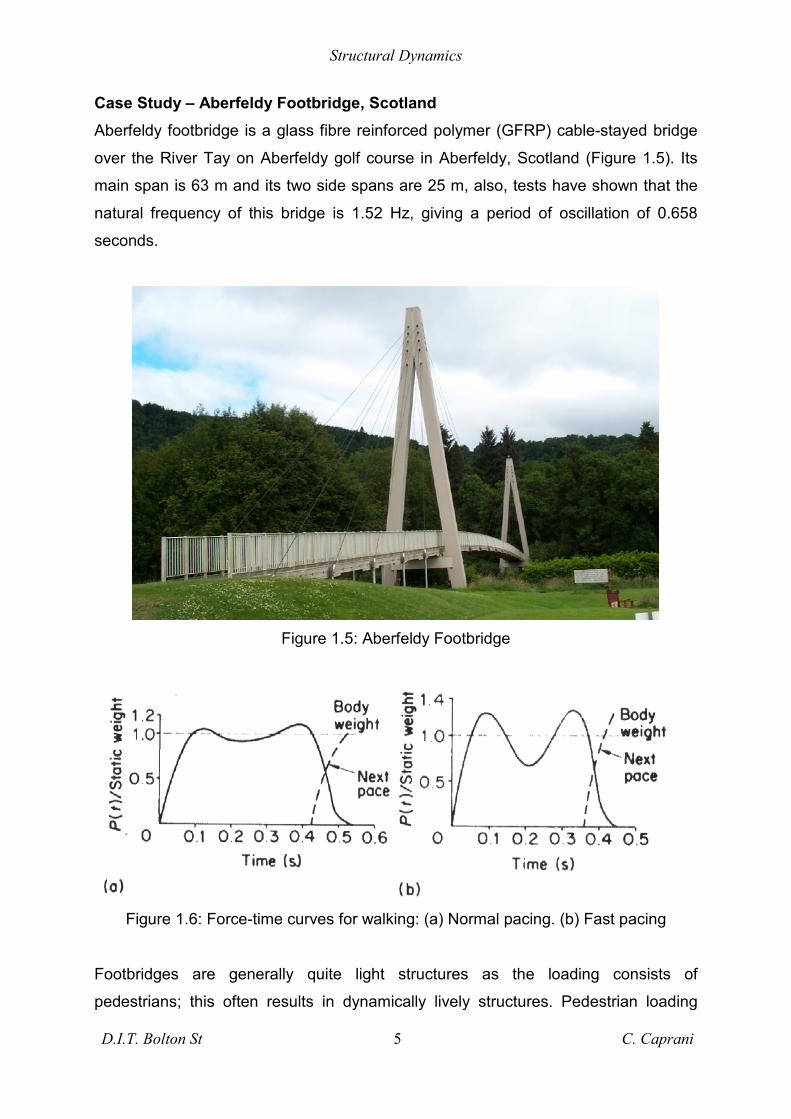
Case Study – Aberfeldy Footbridge, Scotland Aberfeldy footbridge is a glass fibre reinforced polymer (GFRP) cable-stayed bridge

over the River Tay on Aberfeldy golf course in Aberfeldy, Scotland (Figure 1.5). Its

main span is 63 m and its two side spans are 25 m, also, tests have shown that the

natural frequency of this bridge is 1.52 Hz, giving a period of oscillation of 0.658

seconds.

Figure 1.5: Aberfeldy Footbridge

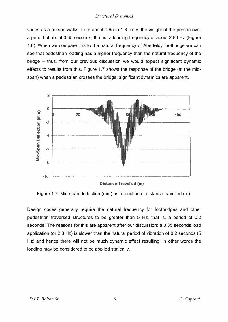
Figure 1.6: Force-time curves for walking: (a) Normal pacing. (b) Fast pacing

Footbridges are generally quite light structures as the loading consists of

pedestrians; this often results in dynamically lively structures. Pedestrian loading

Structural Dynamics


varies as a person walks; from about 0.65 to 1.3 times the weight of the person over

a period of about 0.35 seconds, that is, a loading frequency of about 2.86 Hz (Figure

1.6). When we compare this to the natural frequency of Aberfeldy footbridge we can

see that pedestrian loading has a higher frequency than the natural frequency of the

bridge – thus, from our previous discussion we would expect significant dynamic

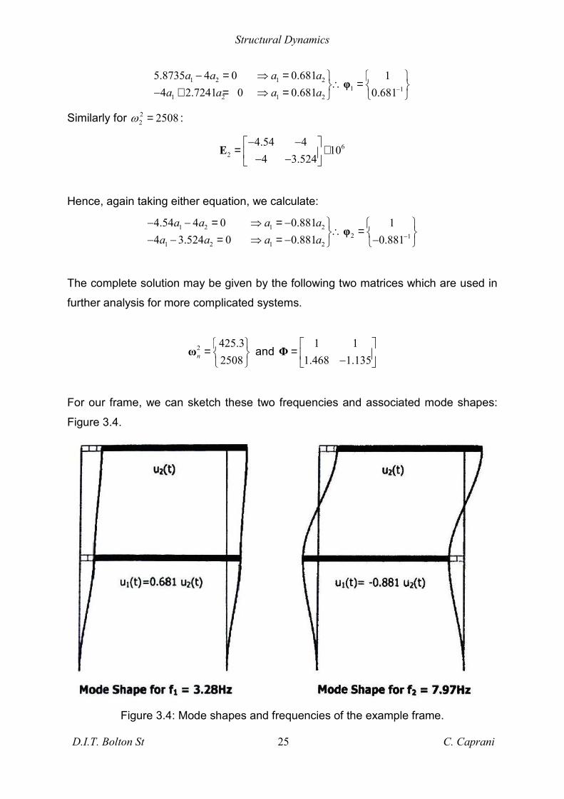
effects to results from this. Figure 1.7 shows the response of the bridge (at the mid-

span) when a pedestrian crosses the bridge: significant dynamics are apparent.

Figure 1.7: Mid-span deflection (mm) as a function of distance travelled (m).

Design codes generally require the natural frequency for footbridges and other

pedestrian traversed structures to be greater than 5 Hz, that is, a period of 0.2

seconds. The reasons for this are apparent after our discussion: a 0.35 seconds load

application (or 2.8 Hz) is slower than the natural period of vibration of 0.2 seconds (5

Hz) and hence there will not be much dynamic effect resulting; in other words the

loading may be considered to be applied statically.

Structural Dynamics


Look again at the frog in Figure 1.1, according to the results obtained so far which

are graphed in Figures 1.3 and 1.4, the frog should oscillate indefinitely. If you have

ever cantilevered a ruler off the edge of a desk and flicked it you would have seen it

vibrate for a time but certainly not indefinitely; buildings do not vibrate indefinitely

after an earthquake; Figure 1.7 shows the vibrations dying down quite soon after the

pedestrian has left the main span of Aberfeldy bridge - clearly there is another action

opposing or “damping” the vibration of structures. Figure 1.8 shows the Undamped

response of our model along with the Damped response; it can be seen that the

oscillations die out quite rapidly – this obviously depends on the level of damping.

Damped and Undamped Response

-25

-20

-15

-10

-5

0

5

10

15

20

25

0 5 10 15 20

Time (s)

Dis

plac

emen

t(m

m)

UndampedDamped

Figure 1.8

Damping occurs in structures due to energy loss mechanisms that exist in the

system. Examples are friction losses at any connection to or in the system and

internal energy losses of the materials due to thermo-elasticity, hysteresis and inter-

granular bonds. The exact nature of damping is difficult to define; fortunately

theoretical damping has been shown to match real structures quite well.

m = 10 kg

k = 100 N/m

Structural Dynamics


2. Single Degree-of-Freedom Systems a. Fundamental Equation of Motion

(a) (b)

Figure 2.1: (a) SDOF system. (b) Free-body diagram of forces

Considering Figure 2.1, the forces resisting the applied loading are considered as:

1. a force proportional to displacement (the usual static stiffness);

2. a force proportional to velocity (the damping force);

3. a force proportional to acceleration (D’Alambert’s inertial force).

We can write the following symbolic equation:

applied stiffness damping inertiaF F F F= + + (2.1)

Noting that:

stiffness

damping

inertia

FFF

kucumu

= = =

(2.2)

that is, stiffness × displacement, damping coefficient × velocity and mass ×

acceleration respectively. Note also that u represents displacement from the

equilibrium position and that the dots over u represent the first and second

derivatives with respect to time. Thus, noting that the displacement, velocity and

acceleration are all functions of time, we have the fundamental equation of motion:

( ) ( ) ( ) ( )mu t cu t ku t F t+ + = (2.3)

This is the standard form of the equation. In the case of free vibration when there is

no external force, ( )F t , we write the alternative formulation:

( )F tmu

cukum

ku(t)

c

( )F t

Structural Dynamics


2( ) 2 ( ) ( ) 0u t u t u tξω ω+ + = (2.4)

which uses the following notation,

2 ;cm

ξω = 2 km

ω = (2.5) and (2.6)

where

;cr

cc

ξ = 2 2crc m kmω= = (2.7) and (2.8)

ω is called the undamped circular natural frequency and its units are radians per

second (rad/s). ξ is the damping ratio which is the ratio of the damping coefficient,

c , to the critical value of the damping coefficient crc ; we will see what these terms

physically mean.

In considering free vibration only, the general solution to (2.4) is of a form

tu Ceλ= (2.9)

When we substitute (2.9) and its derivates into (2.4) we get:

( )2 22 0tCeλλ ξωλ ω+ + = (2.10)

For this to be valid for all values of t, we get the characteristic equation:

2 22 0λ ξωλ ω+ + = (2.11)

the solutions to this equation are the two roots:

2 2 2

1,2

2

2 4 42

1

ωξ ω ξ ωλ

ωξ ω ξ

− ± −=

= − ± −

(2.12)

Therefore the solution depends on the magnitude of ξ relative to 1. We have:

1. 1ξ < : Sub-critical damping or under-damped;

Oscillatory response only occurs when this is the case – as it is for almost all

structures.

2. 1ξ = : Critical damping;

No oscillatory response occurs.

3. 1ξ > : Super-critical damping or over-damped;

No oscillatory response occurs.

Structural Dynamics


b. Free Vibration of Undamped Structures We will examine the case when there is no damping on the SDOF system of Figure

2.1 so 0ξ = in equations (2.4), (2.11) and (2.12) which then become:

2( ) ( ) 0u t u tω+ = (2.13)

2 2 0λ ω+ = (2.14)

1,2 iλ ω= ± (2.15)

respectively, where 1i = − . Using these roots in (2.13) and by using Euler’s

equation we get the general solution:

( ) cos sinu t A t B tω ω= + (2.16)

where A and B are constants to be obtained from the initial conditions of the system

and so:

( ) 00 cos sinuu t u t tω ω

ω = +

(2.17)

where 0u and 0u are the initial displacement and velocity of the system respectively.

Noting that cosine and sine are functions that repeat with period 2π , we see that

( )1 1 2t T tω ω π+ = + (Figure 2.3) and so the undamped natural period of the SDOF

system is:

2T πω

= (2.18)

The natural frequency of the system is got from (1.1), (2.18) and (2.6):

1 12 2

kfT m

ωπ π

= = = (2.19)

and so we have proved (1.2). The importance of this equation is that it shows the

natural frequency of structures to be proportional to km . This knowledge can aid a

designer in addressing problems with resonance in structures: by changing the

stiffness or mass of the structure, problems with dynamic behaviour can be

minimized.

Structural Dynamics


-30

-20

-10

0

10

20

30

0 0.5 1 1.5 2 2.5 3 3.5 4

Time (s)

Dis

plac

emen

t(m

m)

(a)(b)(c)

Figure 2.2: SDOF free vibration response for (a) 0 20mmu = , 0 0u = , (b) 0 0u = ,

0 50mm/su = , and (c) 0 20mmu = , 0 50mm/su = .

Figure 2.2 shows the free-vibration response of a spring-mass system for various

initial states of the system. It can be seen from (b) and (c) that when 0 0u ≠ the

amplitude of displacement is not that of the initial displacement; this is obviously an

important characteristic to calculate. The cosine addition rule may also be used to

show that equation (2.16) can be written in the form:

( )( ) cosu t C tω θ= + (2.20)

where 2 2C A B= + and tan BAθ −= . Using A and B as calculated earlier for the

initial conditions, we then have:

( )( ) cosu t tρ ω θ= + (2.21)

where ρ is the amplitude of displacement and θ is the phase angle, both given by:

2

2 00 ;uuρ

ω = +

0

0

tan uu

θω

−=

(2.22) and (2.23)

The phase angle determines the amount by which ( )u t lags behind the function

cos tω . Figure 2.3 shows the general case.

m = 10 kg

k = 100 N/m

Structural Dynamics


Figure 2.3 Undamped free-vibration response

Examples Example 2.1

A harmonic oscillation test gave the natural frequency of a water tower to be

0.41 Hz. Given that the mass of the tank is 150 tonnes, what deflection will

result if a 50 kN horizontal load is applied? You may neglect the mass of the

tower.

Ans: 50.2 mm

Example 2.2

A 3 m high, 8 m wide single-bay single-storey frame is rigidly jointed with a

beam of mass 5,000 kg and columns of negligible mass and stiffness of EIc =

4.5×103 kNm2. Calculate the natural frequency in lateral vibration and its

period. Find the force required to deflect the frame 25 mm laterally.

Ans: 4.502 Hz; 0.222 sec; 100 kN

Example 2.3

An SDOF system (m = 20 kg, k = 350 N/m) is given an initial displacement of

10 mm and initial velocity of 100 mm/s. (a) Find the natural frequency; (b) the

period of vibration; (c) the amplitude of vibration; and (d) the time at which the

third maximum peak occurs.

Ans: 0.666 Hz; 1.502 sec; 25.91 mm; 3.285 sec.

Structural Dynamics


c. Free Vibration of Damped Structures

Figure 2.4: Response with critical or super-critical damping

When taking account of damping, we noted previously that there are 3, cases but

only when 1ξ < does an oscillatory response ensue. We will not examine the critical

or super-critical cases. Examples are shown in Figure 2.4.

To begin, when 1ξ < (2.12) becomes:

1,2 diλ ωξ ω= − ± (2.24)

where dω is the damped circular natural frequency given by:

21dω ω ξ= − (2.25)

which has a corresponding damped period and frequency of:

2 ;dd

T πω

=2

ddf

ωπ

= (2.26) and (2.27)

The general solution to equation (2.9), using Euler’s formula again, becomes:

( )( ) cos sintd du t e A t B tξω ω ω−= + (2.28)

and again using the initial conditions we get:

0 00( ) cos sint d

d dd

u uu t e u t tξω ξωω ωω

− += +

(2.29)

Structural Dynamics


Using the cosine addition rule again we also have:

( )( ) costdu t e tξωρ ω θ−= + (2.30)

In which

2

2 0 00 ;

d

u uu ξωρω

+= +

0 0

0

tand

u uu

ξωθω−=

(2.31) and (2.32)

Equations (2.28) to (2.32) correspond to those of the undamped case looked at

previously when 0ξ = .

-25

-20

-15

-10

-5

0

5

10

15

20

25

0 0.5 1 1.5 2 2.5 3 3.5 4

Time (s)

Dis

plac

emen

t(m

m)

(a)(b)(c)(d)

Figure 2.5: SDOF free vibration response for:

(a) 0ξ = ; (b) 0.05ξ = ; (c) 0.1ξ = ; and (d) 0.5ξ = .

Figure 2.5 shows the dynamic response of the SDOF model shown. It may be clearly

seen that damping has a large effect on the dynamic response of the system – even

for small values of ξ . We will discuss damping in structures later but damping ratios

for structures are usually in the range 0.5 to 5%. Thus, the damped and undamped

properties of the systems are very similar for these structures.

Figure 2.6 shows the general case of an under-critically damped system.

m = 10 kg

k = 100 N/m

ξ varies

Structural Dynamics


Figure 2.6: General case of an under-critically damped system.

Estimating Damping in Structures

Examining Figure 2.6, we see that two successive peaks, nu and n mu + , m cycles

apart, occur at times nT and ( )n m T+ respectively. Using equation (2.30) we can

get the ratio of these two peaks as:

2expn

n m d

u mu

πξωω+

=

(2.33)

where ( )exp xx e≡ . Taking the natural log of both sides we get the logarithmic

decrement of damping, δ , defined as:

ln 2n

n m d

u mu

ωδ πξω+

= = (2.34)

for low values of damping, normal in structural engineering, we can approximate this:

2mδ πξ≅ (2.35)

thus,

( )exp 2 1 2n

n m

u e m mu

δ πξ πξ+

= ≅ ≅ + (2.36)

and so,

2

n n m

n m

u um u

ξπ

+

+

−≅ (2.37)

Structural Dynamics


This equation can be used to estimate damping in structures with light damping

( 0.2ξ < ) when the amplitudes of peaks m cycles apart is known. A quick way of

doing this, known as the Half-Amplitude Method, is to count the number of peaks it

takes to halve the amplitude, that is 0.5n m nu u+ = . Then, using (2.37) we get:

0.11m

ξ ≅ when 0.5n m nu u+ = (2.38)

Further, if we know the amplitudes of two successive cycles (and so 1m = ), we can

find the amplitude after p cycles from two instances of equation (2.36):

1

p

nn p n

n

uu uu

++

=

(2.39)

Examples Example 2.4

For the frame of Example 2.2, a jack applied a load of 100 kN and then

instantaneously released. On the first return swing a deflection of 19.44 mm

was noted. The period of motion was measured at 0.223 sec. Assuming that

the stiffness of the columns cannot change, find (a) the effective weight of the

beam; (b) the damping ratio; (c) the coefficient of damping; (d) the undamped

frequency and period; and (e) the amplitude after 5 cycles.

Ans: 5,039 kg; 0.04; 11,367 kg·s/m; 4.488 Hz; 0.2228 sec; 7.11 mm.

Example 2.5

From the response time-history of an SDOF system given, (a) estimate the

damped natural frequency; (b) use the half amplitude method to calculate the

damping ratio; and (c) calculate the undamped natural frequency and period.

Ans: 2.24 Hz; 0.0512; 2.236 Hz; 0.447 sec. (see handout sheet for figure)

Example 2.6

Workers’ movements on a platform (8 × 6 m high, m = 200 kN) are causing

large dynamic motions. An engineer investigated and found the natural period

in sway to be 0.9 sec. Diagonal remedial ties (E = 200 kN/mm2) are to be

installed to reduce the natural period to 0.3 sec. What tie diameter is required?

Ans: 28.1 mm.

Structural Dynamics


d. Forced Response of an SDOF System

Figure 2.7: SDOF undamped system subjected to harmonic excitation

So far we have only considered free vibration; the structure has been set vibrating by

an initial displacement for example. We will now consider the case when a time

varying load is applied to the system. We will confine ourselves to the case of

harmonic or sinusoidal loading though there are obviously infinitely many forms that a

time-varying load may take – refer to the references (Appendix - 6.a) for more.

To begin, we note that the forcing function ( )F t has excitation amplitude of 0F and

an excitation circular frequency of Ω and so from the fundamental equation of motion

(2.3) we have:

0( ) ( ) ( ) sinmu t cu t ku t F t+ + = Ω (2.40)

The solution to equation (2.40) has two parts:

• The complementary solution, similar to (2.28), which represents the transient

response of the system which damps out by ( )exp tξω− . The transient response

may be thought of as the vibrations caused by the initial application of the load.

• The particular solution, ( )pu t , representing the steady-state harmonic response

of the system to the applied load. This is the response we will be interested in as

it will account for any resonance between the forcing function and the system.

The particular solution will have the form

( ) cos sinpu t A t B t= Ω + Ω (2.41)

After substitution in (2.40) and separating the equation by sine and cosine terms, we

solve for A and B to get and follow the procedure of (2.21) to get:

( ) ( )sinpu t tρ θ= Ω − (2.42)

mk

u(t)

c

0( ) sinF t F t= Ω

Structural Dynamics


In which

( ) ( )1 22 220 1 2 ;F

kρ β ξβ

− = − +

2

2tan1ξβθβ

=−

(2.43) and (2.44)

where the phase angle is limited to 0 θ π< < and the ratio of the applied load

frequency to the natural undamped frequency is:

βωΩ= (2.45)

the maximum response of the system will come at ( )sin 1t θΩ − = and dividing (2.42)

by the static deflection 0F k we can get the dynamic amplification factor (DAF) of the

system as:

( ) ( )1 22 22DAF 1 2D β ξβ−

≡ = − + (2.46)

11

2Dβ ξ= = (2.47)

Figure 2.8: Variation of DAF with damping and frequency ratios.

Structural Dynamics


Figure 2.8 shows the effect of the frequency ratio β on the DAF. Resonance is the

phenomenon that occurs when the forcing frequency coincides with that of the

natural frequency, 1β = . It can also be seen that for low values of damping, normal

in structures, very high DAFs occur; for example if 0.02ξ = then the dynamic

amplification factor will be 25. For the case of no damping, the DAF goes to infinity -

theoretically at least; equation (2.47).

Measurement of Natural Frequencies

It may be seen from (2.44) that when 1β = , 2θ π= ; this phase relationship allows

the accurate measurements of the natural frequencies of structures. That is, we

change the input frequency Ω in small increments until we can identify a peak

response: the value of Ω at the peak response is then the natural frequency of the

system. Example 2.1 gave the natural frequency based on this type of test.

Examples

Example 2.7

The frame of examples 2.2 and 2.4 has a reciprocating machine put on it. The

mass of this machine is 4 tonnes and is in addition to the mass of the beam.

The machine exerts a periodic force of 8.5 kN at a frequency of 1.75 Hz. (a)

What is the steady-state amplitude of vibration if the damping ratio is 4%? (b)

What would the steady-state amplitude be if the forcing frequency was in

resonance with the structure?

Ans: 2.92 mm; 26.56 mm.

Example 2.8

An air conditioning unit of mass 1,600 kg is place in the middle (point C) of an

8 m long simply supported beam (EI = 8×103 kNm2) of negligible mass. The

motor runs at 300 rpm and produces an unbalanced load of 120 kg. Assuming

a damping ratio of 5%, determine the steady-state amplitude and deflection at

C. What rpm will result in resonance and what is the associated deflection?

Ans: 1.41 mm; 22.34 mm; 206.7 rpm; 36.66 mm.

Structural Dynamics


3. Multi-Degree-of-Freedom Systems a. General Case (based on 2DOF)

(a)

(b) (c)

Figure 3.1: (a) 2DOF system. (b) and (c) Free-body diagrams of forces

Considering Figure 3.1, we can see that the forces that act on the masses are similar

to those of the SDOF system but for the fact that the springs, dashpots, masses,

forces and deflections may all differ in properties. Also, from the same figure, we can

see the interaction forces between the masses will result from the relative deflection

between the masses; the change in distance between them.

For each mass, 0xF =∑ , hence:

( ) ( )1 1 1 1 1 1 2 1 2 2 1 2 1m u c u k u c u u k u u F+ + + − + − = (3.1)

( ) ( )2 2 2 2 1 2 2 1 2m u c u u k u u F+ − + − = (3.2)

In which we have dropped the time function indicators and allowed u∆ and u∆ to

absorb the directions of the interaction forces. Re-arranging we get:

( ) ( ) ( ) ( )( ) ( ) ( ) ( )

1 1 1 1 2 2 2 1 1 2 2 2 1

2 2 1 2 2 2 1 2 2 2 2

u m u c c u c u k k u k F

u m u c u c u k u k F

+ + + − + + + − =

+ − + + − + =

(3.3)

2F2 2m u

2c u⋅ ∆

2k u⋅∆2m

1m

1( )u t

1( )F t

2m

2 ( )F t

2 ( )u t

1k

1c

2k

2c

1 1m u

1 1c u

1 1k u1m

1F

2c u⋅ ∆

2k u⋅∆

Structural Dynamics


This can be written in matrix form:

1 1 1 2 2 1 1 2 2 1 1

2 2 2 2 2 2 2 2 2

00m u c c c u k k k u F

m u c c u k k u F+ − + −

+ + = − −

(3.4)

Or another way:

Mu+Cu +Ku = F (3.5)

where:

M is the mass matrix (diagonal matrix);

u is the vector of the accelerations for each DOF;

C is the damping matrix (symmetrical matrix);

u is the vector of velocity for each DOF;

K is the stiffness matrix (symmetrical matrix);

u is the vector of displacements for each DOF;

F is the load vector.

Equation (3.5) is quite general and reduces to many forms of analysis:

- Free vibration:

Mu+Cu +Ku = 0 (3.6)

- Undamped free vibration:

Mu+Ku = 0 (3.7)

- Undamped forced vibration:

Mu+Ku = F (3.8)

- Static analysis:

Ku = F (3.9)

We will restrict our attention to the case of undamped free-vibration – equation (3.7) -

as the inclusion of damping requires an increase in mathematical complexity which

would distract from our purpose.

Structural Dynamics


b. Free-Undamped Vibration of 2DOF Systems The solution to (3.7) follows the same methodology as for the SDOF case; so

following that method (equation (2.42)), we propose a solution of the form:

( )sin tω φ+u = a (3.10)

where a is the vector of amplitudes corresponding to each degree of freedom. From

this we get:

( )2 2sin tω ω φ ω− + = −u = a u (3.11)

Then, substitution of (3.10) and (3.11) into (3.7) yields:

( ) ( )2 sin sint tω ω φ ω φ− + +Ma +Ka = 0 (3.12)

Since the sine term is constant for each term:

2ω − K M a = 0 (3.13)

We note that in a dynamics problem the amplitudes of each DOF will be non-zero,

hence, ≠a 0 in general. In addition we see that the problem is a standard

eigenvalues problem. Hence, by Cramer’s rule, in order for (3.13) to hold the

determinant of 2ω−K M must then be zero:

2 0ω−K M = (3.14)

For the 2DOF system, we have:

( )2 2 2 22 1 1 2 2 2 0k k m k m kω ω ω − + − − − = K M = (3.15)

Expansion of (3.15) leads to an equation in 2ω called the characteristic polynomial of

the system. The solutions of 2ω to this equation are the eigenvalues of 2ω − K M .

There will be two solutions or roots of the characteristic polynomial in this case and

an n-DOF system has n solutions to its characteristic polynomial. In our case, this

means there are two values of 2ω ( 21ω and 2

2ω ) that will satisfy the relationship; thus

there are two frequencies for this system (the lowest will be called the fundamental

frequency). For each 2nω substituted back into (3.13), we will get a certain amplitude

vector na . This means that each frequency will have its own characteristic displaced

shape of the degrees of freedoms called the mode shape. However, we will not know

the absolute values of the amplitudes as it is a free-vibration problem; hence we

Structural Dynamics


express the mode shapes as a vector of relative amplitudes, nφ , relative to, normally,

the first value in na .

As we will see in the following example, the implication of the above is that MDOF

systems vibrate, not just in the fundamental mode, but also in higher harmonics.

From our analysis of SDOF systems it’s apparent that should any loading coincide

with any of these harmonics, large DAF’s will result (Section 2.d). Thus, some modes

may be critical design cases depending on the type of harmonic loading as will be

seen later.

Example of a 2DOF System The two-storey building shown (Figure

3.2) has very stiff floor slabs relative to the

supporting columns. Calculate the natural

frequencies and mode shapes.

3 24.5 10 kNmcEI = ×

Figure 3.2: Shear frame problem.

Figure 3.3: 2DOF model of the shear frame.

We will consider the free lateral vibrations of the two-storey shear frame idealised as

in Figure 3.3. The lateral, or shear stiffness of the columns is:

1m

1( )u t

2m

2 ( )u t

1k 2k

Structural Dynamics


1 2 3

6

3

6

122

2 12 4.5 103

4 10 N/m

cEIk k kh

k

= = = × × ×

∴ =

= ×

The characteristic polynomial is as given in (3.15) so we have:

6 2 6 2 12

6 4 10 2 12

8 10 5000 4 10 3000 16 10 0

15 10 4.4 10 16 10 0

ω ω

ω ω

× − × − − × = ∴ × − × + × =

This is a quadratic equation in 2ω and so can be solved using 615 10a = × ,104.4 10b = − × and 1216 10c = × in the usual expression

22 4

2b b ac

aω − ± −=

Hence we get 21 425.3ω = and 2

2 2508ω = . This may be written:

2 425.32508n

=

ω hence 20.650.1n

=

ω rad/s and 3.287.972

n

π

= =

ωf Hz

To solve for the mode shapes, we will use the appropriate form of the equation of

motion, equation (3.13): 2ω − K M a = 0 . First solve for the 2ω = − E K M matrix

and then solve Ea = 0 for the amplitudes na . Then, form nφ .

In general, for a 2DOF system, we have: 2

1 2 2 12 1 2 1 22

2 2 2 2 2 2

00

nn n

n

k k k m k k m kk k m k k m

ωω

ω+ − + − −

= − = − − − E

For 21 425.3ω = :

61

5.8735 410

4 2.7241−

= × − E

Hence

161 1

2

5.8735 4 010

4 2.7241 0aa

− = = −

E a

Taking either equation, we calculate:

Structural Dynamics


1 2 1 21 1

1 2 1 2

5.8735 4 0 0.681 14 2.7241 0 0.681 0.681

a a a aa a a a −

− = ⇒ = ∴ = − + = ⇒ = φ

Similarly for 22 2508ω = :

62

4.54 410

4 3.524− −

= × − − E

Hence, again taking either equation, we calculate:

1 2 1 22 1

1 2 1 2

4.54 4 0 0.881 14 3.524 0 0.881 0.881

a a a aa a a a −

− − = ⇒ = − ∴ = − − = ⇒ = − − φ

The complete solution may be given by the following two matrices which are used in

further analysis for more complicated systems.

2 425.32508n

=

ω and 1 1

1.468 1.135

= − Φ

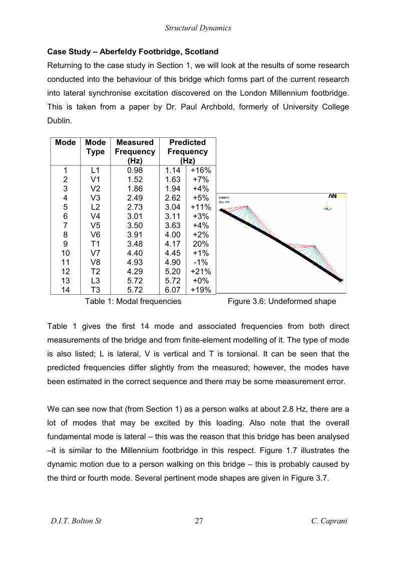
For our frame, we can sketch these two frequencies and associated mode shapes:

Figure 3.4.

Figure 3.4: Mode shapes and frequencies of the example frame.

Structural Dynamics


Larger and more complex structures will have many degrees of freedom and hence

many natural frequencies and mode shapes. There are different mode shapes for

different forms of deformation; torsional, lateral and vertical for example. Periodic

loads acting in these directions need to be checked against the fundamental

frequency for the type of deformation; higher harmonics may also be important.

As an example; consider a 2DOF idealisation of a cantilever which assumes stiffness

proportional to the static deflection at 0.5L and L as well as half the cantilever mass

‘lumped’ at the midpoint and one quarter of it lumped at the tip. The mode shapes are

shown in Figure 3.5. In Section 4(a) we will see the exact mode shape for this – it is

clear that the approximation is rough; but, with more DOFs it will approach a better

solution.

Mode 1Mode 2

Figure 3.5: Lumped mass, 2DOF idealisation of a cantilever.

Structural Dynamics


Case Study – Aberfeldy Footbridge, Scotland Returning to the case study in Section 1, we will look at the results of some research

conducted into the behaviour of this bridge which forms part of the current research

into lateral synchronise excitation discovered on the London Millennium footbridge.

This is taken from a paper by Dr. Paul Archbold, formerly of University College

Dublin.

Table 1 gives the first 14 mode and associated frequencies from both direct

measurements of the bridge and from finite-element modelling of it. The type of mode

is also listed; L is lateral, V is vertical and T is torsional. It can be seen that the

predicted frequencies differ slightly from the measured; however, the modes have

been estimated in the correct sequence and there may be some measurement error.

We can see now that (from Section 1) as a person walks at about 2.8 Hz, there are a

lot of modes that may be excited by this loading. Also note that the overall

fundamental mode is lateral – this was the reason that this bridge has been analysed

–it is similar to the Millennium footbridge in this respect. Figure 1.7 illustrates the

dynamic motion due to a person walking on this bridge – this is probably caused by

the third or fourth mode. Several pertinent mode shapes are given in Figure 3.7.

Mode Mode Type

Measured Frequency

(Hz)

Predicted Frequency

(Hz) 1 L1 0.98 1.14 +16% 2 V1 1.52 1.63 +7% 3 V2 1.86 1.94 +4% 4 V3 2.49 2.62 +5% 5 L2 2.73 3.04 +11% 6 V4 3.01 3.11 +3% 7 V5 3.50 3.63 +4% 8 V6 3.91 4.00 +2% 9 T1 3.48 4.17 20%

10 V7 4.40 4.45 +1% 11 V8 4.93 4.90 -1% 12 T2 4.29 5.20 +21% 13 L3 5.72 5.72 +0% 14 T3 5.72 6.07 +19%

Table 1: Modal frequencies Figure 3.6: Undeformed shape

Structural Dynamics


Mode 1:

1st Lateral mode

1.14 Hz

Mode 2:

1st Vertical mode

1.63 Hz

Mode 3:

2nd Vertical mode

1.94 Hz

Mode 9:

1st Torsional mode

4.17 Hz

Figure 3.7: Various Modes of Aberfeldy footbridge.

Structural Dynamics


4. Continuous Structures a. Exact Analysis for Beams General Equation of Motion

Figure 4.1: Basic beam subjected to dynamic loading: (a) beam properties and

coordinates; (b) resultant forces acting on the differential element.

In examining Figure 4.1, as with any continuous structure, it may be seen that any

differential element will have an associated stiffness and deflection – which changes

with time – and hence a different acceleration. Thus, any continuous structure has an

infinite number of degrees of freedom. Discretization into an MDOF structure is

certainly an option and is the basis for finite-element dynamic analyses; the more

DOF’s used the more accurate the model (Section 3.b). For some basic structures

though, the exact behaviour can be explicitly calculated. We will limit ourselves to

free-undamped vibration of beams that are thin in comparison to their length. A

general expression can be derived and from this, several usual cases may be

established.

Structural Dynamics


Figure 4.2: Instantaneous dynamic deflected position.

Consider the element A of Figure 4.1(b); 0yF =∑ , hence:

( ) ( ) ( ),, , 0I

V x tp x t dx dx f x t dx

x∂

− − =∂

(4.1)

after having cancelled the common ( ),V x t shear term. The resultant transverse

inertial force is (mass × acceleration; assuming constant mass):

( ) ( )2

2

,,I

v x tf x t dx mdx

t∂

=∂

(4.2)

Thus we have, after dividing by the common dx term:

( ) ( ) ( )2

2

, ,,

V x t v x tp x t m

x t∂ ∂

= −∂ ∂

(4.3)

which, with no acceleration, is the usual static relationship between shear force and

applied load. By taking moments about the point A on the element, and dropping

second order and common terms, we get the usual expression:

( ) ( ),,

M x tV x t

x∂

=∂

(4.4)

Differentiating this with respect to x and substituting into (4.3), in addition to the

relationship 2

2vM EI x

∂=∂

(which assumes that the beam is of constant stiffness):

( ) ( ) ( )4 2

4 2

, ,,

v x t v x tEI m p x t

x t∂ ∂

+ =∂ ∂

(4.5)

With free vibration this is:

( ) ( )4 2

4 2

, ,0

v x t v x tEI m

x t∂ ∂

+ =∂ ∂

(4.6)

Structural Dynamics


General Solution for Free-Undamped Vibration Examination of equation (4.6) yields several aspects:

• It is separated into spatial ( x ) and temporal ( t ) terms and we may assume that

the solution is also;

• It is a fourth-order differential in x ; hence we will need four spatial boundary

conditions to solve – these will come from the support conditions at each end;

• It is a second order differential in t and so we will need two temporal initial

conditions to solve – initial deflection and velocity at a point for example.

To begin, assume the solution is of a form of separated variables:

( ) ( ) ( ),v x t x Y tφ= (4.7)

where ( )xφ will define the deformed shape of the beam and ( )Y t the amplitude of

vibration. Inserting the assumed solution into (4.6) and collecting terms we have:

( )

( )( )

( )4 22

4 2

1 1 constantx Y tEI

m x x Y t tφ

ωφ

∂ ∂= − = =

∂ ∂ (4.8)

This follows as the terms each side of the equals are functions of x and t separately

and so must be constant. Hence, each function type (spatial or temporal) is equal to 2ω and so we have:

( ) ( )4

24

xEI m x

xφ

ω φ∂

=∂

(4.9)

( ) ( )2 0Y t Y tω+ = (4.10)

Equation (4.10) is the same as for an SDOF system (equation (2.4)) and so the

solution must be of the same form (equation (2.17)):

( ) 00 cos sinYY t Y t tω ω

ω

= +

(4.11)

In order to evaluate ω we will use equation (4.9) and we introduce:

2

4 mEIωα = (4.12)

And assuming a solution of the form ( ) exp( )x G sxφ = , substitution into (4.9) gives:

( ) ( )4 4 exp 0s G sxα− = (4.13)

There are then four roots for s and when each is put into (4.13) and added we get:

( ) ( ) ( ) ( ) ( )1 2 3 4exp exp exp expx G i x G i x G x G xφ α α α α= + − + + − (4.14)

Structural Dynamics


In which the G ’s may be complex constant numbers, but, by using Euler’s

expressions for cos, sin, sinh and cosh we get:

( ) ( ) ( ) ( ) ( )1 2 3 4sin cos sinh coshx A x A x A x A xφ α α α α= + + + − (4.15)

where the A ’s are now real constants; three of which may be evaluated through the

boundary conditions; the fourth however is arbitrary and will depend on ω .

Simply-supported Beam

Figure 4.3: First three mode shapes and frequency parameters for an s-s beam.

The boundary conditions consist of zero deflection and bending moment at each end:

( ) ( )2

20, 0 and 0, 0vv t EI tx∂

= =∂

(4.16)

( ) ( )2

2, 0 and , 0vv L t EI L tx∂

= =∂

(4.17)

Substituting (4.16) into equation (4.14) we find 2 4 0A A= = . Similarly, (4.17) gives:

( )( )

1 3

2 21 3

sin( ) sinh( ) 0

'' sin( ) sinh( ) 0

L A L A L

L A L A L

φ α α

φ α λ α α

= + =

= − + =(4.18)

from which, we get two possibilities:

Structural Dynamics


3

1

0 2 sinh( )0 sin( )

A LA L

αα

=

=(4.19)

however, since sinh( )xλ is never zero, 3A must be, and so the non-trivial solution

1 0A ≠ must give us:

sin( ) 0Lα = (4.20)

which is the frequency equation and is only satisfied when L nλ π= . Hence, from

(4.12) we get:

2

nn EIL mπω =

(4.21)

and the corresponding modes shapes are therefore:

( ) 1 sinnn xx A

Lπφ =

(4.22)

where 1A is arbitrary and normally taken to be unity. We can see that there are an

infinite number of frequencies and mode shapes ( n →∞ ) as we would expect from

an infinite number of DOFs. The first three mode shapes and frequencies are shown

in Figure 4.3.

Cantilever Beam

This example is important as it describes the sway behaviour of tall buildings. The

boundary conditions consist of:

( ) ( )0, 0 and 0, 0vv t tx∂

= =∂

(4.23)

( ) ( )2 3

2 3, 0 and , 0v vEI L t EI L tx x∂ ∂

= =∂ ∂

(4.24)

Which represent zero displacement and slope at the support and zero bending

moment and shear at the tip. Substituting (4.23) into equation (4.14) we get 4 2A A= −

and 3 1A A= − . Similarly, (4.24) gives:

( )( )

2 2 2 21 2 3 4

3 3 3 31 2 3 4

'' sin( ) cos( ) sinh( ) cosh( ) 0

''' cos( ) sin( ) cosh( ) sinh( ) 0

L A L A L A L A L

L A L A L A L A L

φ α α α α α α α α

φ α α α α α α α α

= − − + + =

= − + + + =(4.25)

where a prime indicates a derivate of x , and so we find:

( ) ( )( ) ( )

1 2

1 2

sin( ) sinh( ) cos( ) cosh( ) 0

cos( ) cosh( ) sin( ) sinh( ) 0

A L L A L L

A L L A L L

α α α α

α α α α

+ + + =

+ + − + =(4.26)

Structural Dynamics


Solving for 1A and 2A we find:

( ) ( )( )

( ) ( ) ( )

21

22

cos( ) cosh( ) sin( ) sinh( ) sin( ) sinh( ) 0

cos( ) cosh( ) sin( ) sinh( ) sin( ) sinh( ) 0

A L L L L L L

A L L L L L L

α α α α α α

α α α α α α

+ − + − + = + − + − + =

(4.27)

In order that neither 1A and 2A are zero, the expression in the brackets must be zero

and we are left with the frequency equation:

cos( )cosh( ) 1 0L Lα α + = (4.28)

The mode shape is got by expressing 2A in terms of 1A :

2 1sin( ) sinh( )cos( ) cosh( )

L LA AL L

α αα α

+= −

+(4.29)

and the modes shapes are therefore:

( ) ( )1sin( ) sinh( )sin( ) sinh( ) cosh( ) cos( )cos( ) cosh( )n

L Lx A x x x xL L

α αφ α α α αα α

+= − + − +

(4.30)

where again 1A is arbitrary and normally taken to be unity. We can see from (4.28)

that it must be solved numerically for the corresponding values of Lα The natural

frequencies are then got from (4.21) with the substitution of Lα for nπ . The first

three mode shapes and frequencies are shown in Figure 4.4.

Figure 4.4: First three mode shapes and frequency parameters for a cantilever.

Structural Dynamics


b. Approximate Analysis – Bolton’s Method

We will now look at a simplified method that requires an understanding of dynamic

behaviour but is very easy to implement. The idea is to represent, through various

manipulations of mass and stiffness, any complex structure as a single SDOF system

which is easily solved via an implementation of equation (1.2):

12

E

E

KfMπ

= (4.31)

in which we have equivalent SDOF stiffness and mass terms.

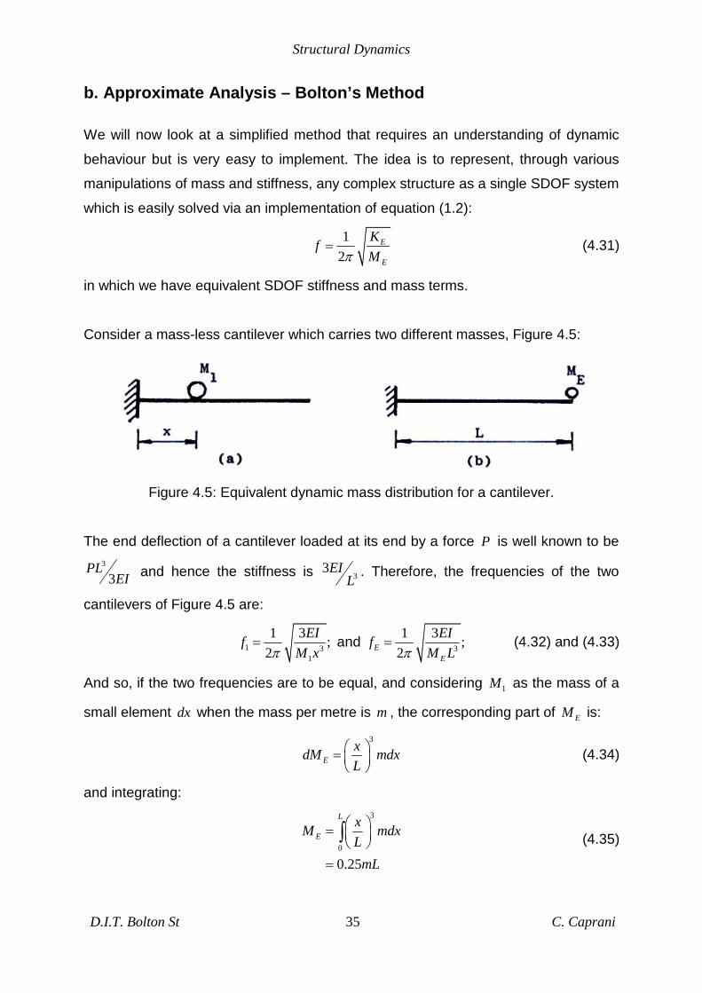
Consider a mass-less cantilever which carries two different masses, Figure 4.5:

Figure 4.5: Equivalent dynamic mass distribution for a cantilever.

The end deflection of a cantilever loaded at its end by a force P is well known to be 3

3PL

EI and hence the stiffness is 33EI

L . Therefore, the frequencies of the two

cantilevers of Figure 4.5 are:

1 31

1 3 ;2

EIfM xπ

= and 3

1 3 ;2E

E

EIfM Lπ

= (4.32) and (4.33)

And so, if the two frequencies are to be equal, and considering 1M as the mass of a

small element dx when the mass per metre is m , the corresponding part of EM is:

3

ExdM mdxL

=

(4.34)

and integrating:

3

0

0.25

L

ExM mdxL

mL

=

=

∫ (4.35)

Structural Dynamics


Therefore the cantilever with self-mass uniformly distributed along its length vibrates

at the same frequency as would the mass-less cantilever loaded with a mass one

quarter its actual mass. This answer is not quite correct but is within 5%; it ignores

the fact that every element affects the deflection (and hence vibration) of every other

element. The answer is reasonable for design though.

Figure 4.6: Equivalent dynamic mass distribution for an s-s beam

Similarly for a simply supported beam, we have an expression for the deflection at a

point:

( )22

3x

Px L xEIL

δ−

= (4.36)

and so its stiffness is:

( )22

3x

EILKx L x

=−

(4.37)

Considering Figure 4.6, we see that, from (4.31):

( )2 32

1

3 48

E

EIL EIL Mx L x M

=−

(4.38)

and as the two frequencies are to be equal:

( )2

24

0

16

8 /15

L

E

L xM x mdx

LmL

−=

=

∫ (4.39)

which is about half of the self-mass as we might have guessed.

Proceeding in a similar way we can find equivalent spring stiffnesses and masses for

usual forms of beams as given in Table 1. Table 4.1 however, also includes a

Structural Dynamics


refinement of the equivalent masses based on the known dynamic deflected shape

rather than the static deflected shape.

Table 4.1: Bolton’s table for equivalent mass, stiffnesses and relative amplitudes.

Figure 4.7: Effective SDOFs: (a) neglecting relative amplitude; (b) including relative

amplitude.

Structural Dynamics


In considering continuous beams, the continuity over the supports requires all the

spans to vibrate at the same frequency for each of its modes. Thus we may consider

summing the equivalent masses and stiffnesses for each span and this is not a bad

approximation. It is equivalent to the SDOF model of Figure 4.7(a). But, if we allowed

for the relative amplitude between the different spans, we would have the model of

Figure 4.7(b) which would be more accurate – especially when there is a significant

difference in the member stiffnesses and masses: long heavy members will have

larger amplitudes than short stiff light members due to the amount of kinetic energy

stored. Thus, the stiffness and mass of each span must be weighted by its relative

amplitude before summing. Consider the following examples of the beam shown in

Figure 4.8; the exact multipliers are known to be 10.30, 13.32, 17.72, 21.67, 40.45,

46.10, 53.89 and 60.53 for the first eight modes.

Figure 4.8: Continuous beam of Examples 1 to 3.

Example 1: Ignoring relative amplitude and refined ME

From Table 4.1, and the previous discussion:

( )3 48 3 101.9EEIKL

= × +∑ ; and 8 1315 2EM mL = × +

∑ ,

and applying (4.31) we have: ( ) 4

110.822

EIfmLπ

=

The multiplier in the exact answer is 10.30: an error of 5%.

Example 2: Including relative amplitude and refined ME

From Table 4.1 and the previous discussion, we have:

3 3 3

48 101.93 1 0.4108 185.9EEI EI EIK

L L L= × × + × =∑

Structural Dynamics


3 0.4928 1 0.4299 0.4108 1.655EM mL mL mL= × × + × =∑and applying (4.31) we have:

( ) 4

110.602

EIfmLπ

=

The multiplier in the exact answer is 10.30: a reduced error of 2.9%.

Example 3: Calculating the frequency of a higher mode

Figure 4.9: Assumed mode shape for which the frequency will be found.

The mode shape for calculation is shown in Figure 4.7. We can assume supports at

the midpoints of each span as they do not displace in this mode shape. Hence we

have seven simply supported half-spans and one cantilever half-span, so from Table

4.1 we have:

( ) ( )

( ) ( )

3 3

3

48 101.97 1 0.41080.5 0.5

3022.9

7 0.4928 0.5 1 0.4299 0.5 0.4108

1.813

E

E

EI EIKL LEIL

M m L m LmL

= × × + ×

=

= × × + ×

=

∑

∑

again, applying (4.31), we have:

( ) 4

140.82

EIfmLπ

=

The multiplier in the exact answer is 40.45: and error of 0.9%.

Mode Shapes and Frequencies Section 2.d described how the DAF is very large when a force is applied at the

natural frequency of the structure; so for any structure we can say that when it is

vibrating at its natural frequency it has very low stiffness – and in the case of no

Structural Dynamics


damping: zero stiffness. Higher modes will have higher stiffnesses but stiffness may

also be recognised in one form as

1MEI R

= (4.40)

where R is the radius of curvature and M is bending moment. Therefore, smaller

stiffnesses have a larger R and larger stiffnesses have a smaller R . Similarly then,

lower modes have a larger R and higher modes have a smaller R . This enables us

to distinguish between modes by their frequencies. Noting that a member in single

curvature (i.e. no point of contraflexure) has a larger R than a member in double

curvature (1 point of contraflexure) which in turn has a larger R than a member in

triple curvature (2 points of contraflexure), we can distinguish modes by deflected

shapes. Figures 4.3 and 4.4 illustrate this clearly.

Figure 4.10: Typical modes and reduced structures.

An important fact may be deduced from Figure 4.10 and the preceding arguments: a

continuous beam of any number of identical spans has the same fundamental

frequency as that of one simply supported span: symmetrical frequencies are

similarly linked. Also, for non-identical spans, symmetry may exist about a support

and so reduced structures may be used to estimate the frequencies of the total

structure; reductions are shown in Figure 4.10(b) and (d) for symmetrical and anti-

symmetrical modes.

Structural Dynamics


Examples: Example 4.1:

Calculate the first natural frequency of a simply supported bridge of mass 7

tonnes with a 3 tonne lorry at its quarter point. It is known that a load of 10 kN

causes a 3 mm deflection.

Ans.: 3.95Hz.

Example 4.2:

Calculate the first natural frequency of a 4 m long cantilever (EI = 4,320 kNm2)

which carries a mass of 500 kg at its centre and has self weight of 1200 kg.

Ans.: 3.76 Hz.

Example 4.3:

What is the fundamental frequency of a 3-span continuous beam of spans 4, 8

and 5 m with constant EI and m? What is the frequency when EI = 6×103

kNm2 and m = 150 kg/m?

Ans.: 6.74 Hz.

Example 4.4:

Calculate the first and second natural frequencies of a two-span continuous

beam; fixed at A and on rollers at B and C. Span AB is 8 m with flexural

stiffness of 2EI and a mass of 1.5m. Span BC is 6 m with flexural stiffness EI

and mass m per metre. What are the frequencies when EI = 4.5×103 kNm2

and m = 100 kg/m?

Ans.: 9.3 Hz; ? Hz.

Example 4.5:

Calculate the first and second natural frequencies of a 4-span continuous

beam of spans 4, 5, 4 and 5 m with constant EI and m? What are the

frequencies when EI = 4×103 kNm2 and m = 120 kg/m? What are the new

frequencies when support A is fixed? Does this make it more or less

susceptible to human-induced vibration?

Ans.: ? Hz; ? Hz.

Structural Dynamics


5. Practical Design Considerations a. Human Response to Dynamic Excitation

Figure 5.1: Equal sensation contours for vertical vibration

The response of humans to vibrations is a complex phenomenon involving the

variables of the vibrations being experienced as well as the perception of it. It has

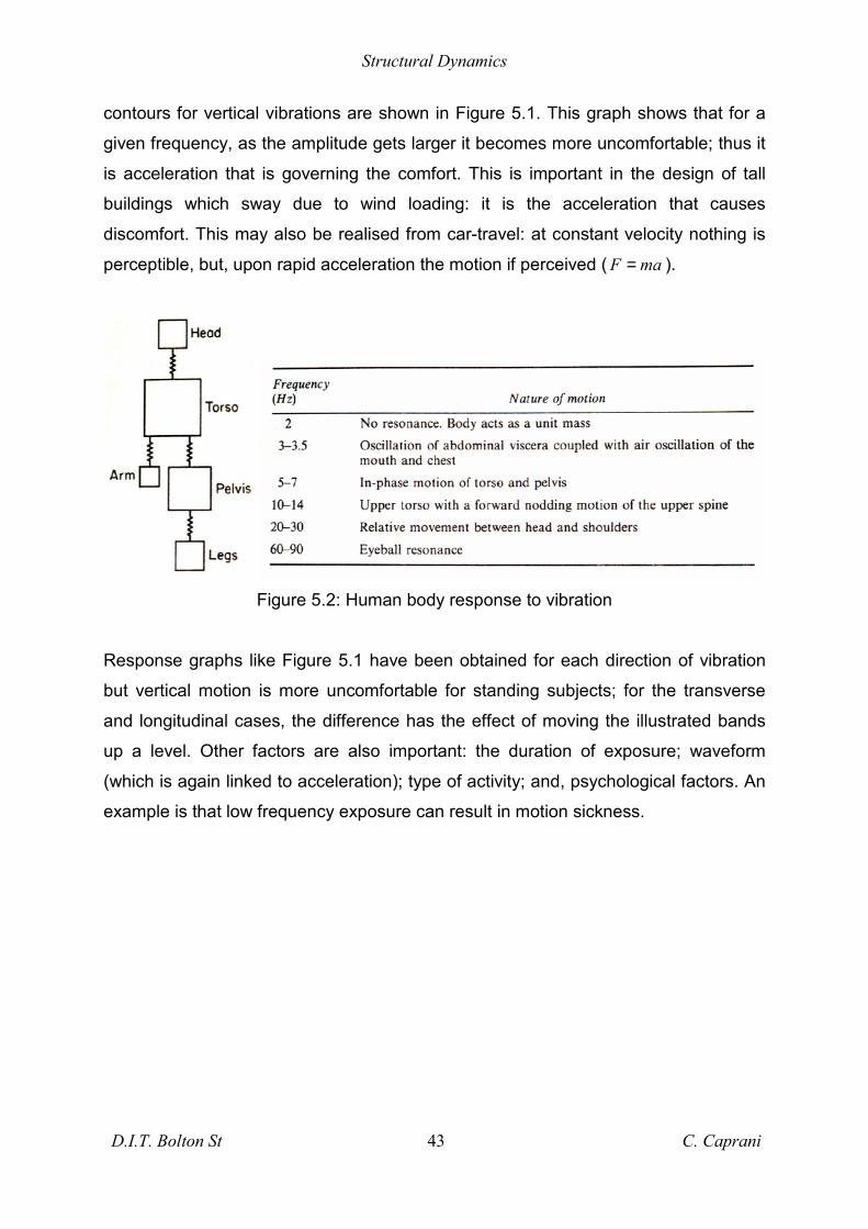
been found that the frequency range between 2 and 30 Hz is particularly

uncomfortable because of resonance with major body parts (Figure 5.2). Sensation

Structural Dynamics


contours for vertical vibrations are shown in Figure 5.1. This graph shows that for a

given frequency, as the amplitude gets larger it becomes more uncomfortable; thus it

is acceleration that is governing the comfort. This is important in the design of tall

buildings which sway due to wind loading: it is the acceleration that causes

discomfort. This may also be realised from car-travel: at constant velocity nothing is

perceptible, but, upon rapid acceleration the motion if perceived ( F ma= ).

Figure 5.2: Human body response to vibration

Response graphs like Figure 5.1 have been obtained for each direction of vibration

but vertical motion is more uncomfortable for standing subjects; for the transverse

and longitudinal cases, the difference has the effect of moving the illustrated bands

up a level. Other factors are also important: the duration of exposure; waveform

(which is again linked to acceleration); type of activity; and, psychological factors. An

example is that low frequency exposure can result in motion sickness.

Structural Dynamics


b. Crowd/Pedestrian Dynamic Loading Lightweight Floors

Figure 5.3: Recommended vibration limits for light floors.

Vibration limits for light floors from the 1984 Canadian Standard is shown in Figure

5.2; the peak acceleration is got from:

( )0 0.9 2 Ia fM

π= (5.1)

where I is the impulse (the area under the force time graph) and is about 70 Ns and

M is the equivalent mass of the floor which is about 40% of the distributed mass.

This form of approach is to be complemented by a simple analysis of an equivalent

SDOF system. Also, as seen in Section 1, by keeping the fundamental frequency

above 5 Hz, human loading should not be problematic.

Structural Dynamics


Crowd Loading This form of loading occurs in grandstands and similar structures where a large

number of people are densely packed and will be responding to the same stimulus.

Coordinated jumping to the beat of music, for example, can cause a DAF of about

1.97 at about 2.5 Hz. Dancing, however, normally generates frequencies of 2 – 3 Hz.

Once again, by keeping the natural frequency of the structure above about 5 Hz no

undue dynamic effects should be noticed.

In the transverse or longitudinal directions, allowance should also be made due to the

crowd-sway that may accompany some events a value of about 0.3 kN per metre of

seating parallel and 0.15 kN perpendicular to the seating is an approximate method

for design.

Staircases can be subject to considerable dynamic forces as running up or down

such may cause peak loads of up to 4-5 times the persons bodyweight over a period

of about 0.3 seconds – the method for lightweight floors can be applied to this

scenario.

Footbridges As may be gathered from the Case Studies of the Aberfeldy Bridge, the problem is

complex, however some rough guidelines are possible. Once again controlling the

fundamental frequency is important; the lessons of the London Millennium and the

Tacoma Narrows bridges need to be heeded though: dynamic effects may occur in

any direction or mode that can be excited by any form of loading.

An approximate method for checking foot bridges is the following:

max stu u Kψ= (5.2)

where stu is the static deflection under the weight of a pedestrian at the point of

maximum deflection; K is a configuration factor for the type of structure (given in

Table 5.1); and ψ is the dynamic response factor got again from Figure 5.4. The

maximum acceleration is then got as 2max maxu uω= (see equations (2.30) and (3.11)

Structural Dynamics


for example, note: 2 2 fω π= ). This is then compared to a rather simple rule that the

maximum acceleration of footbridge decks should not exceed 0.5 f± .

Alternatively, BD 37/01 states:

“For superstructures for which the fundamental natural frequency of vibration

exceeds 5Hz for the unloaded bridge in the vertical direction and 1.5 Hz for

the loaded bridge in the horizontal direction, the vibration serviceability

requirement is deemed to be satisfied.” – Appendix B.1 General.

Adhering to this clause (which is based on the discussion of Section 1’s Case Study)

is clearly the easiest option.

Also, note from Figure 5.4 the conservative nature of the damping assumed, which,

from equation (2.35) can be seen to be so based on usual values of damping in

structures.

Table 5.1: Configuration factors for footbridges.

Table 5.2: Values of the logarithmic decrement for different bridge types.

Structural Dynamics


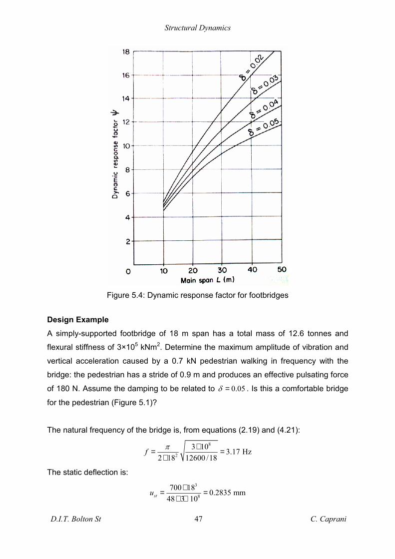
Figure 5.4: Dynamic response factor for footbridges

Design Example

A simply-supported footbridge of 18 m span has a total mass of 12.6 tonnes and

flexural stiffness of 3×105 kNm2. Determine the maximum amplitude of vibration and

vertical acceleration caused by a 0.7 kN pedestrian walking in frequency with the

bridge: the pedestrian has a stride of 0.9 m and produces an effective pulsating force

of 180 N. Assume the damping to be related to 0.05δ = . Is this a comfortable bridge

for the pedestrian (Figure 5.1)?

The natural frequency of the bridge is, from equations (2.19) and (4.21):

8

2

3 10 3.17 Hz2 18 12600 /18

f π ×= =×

The static deflection is:

3

8

700 18 0.2835 mm48 3 10stu ×= =

× ×

Structural Dynamics


Table 5.1 gives 1K = and Figure 5.4 gives 6.8ψ = and so, by (5.2) we have:

max 0.2835 1.0 6.8 1.93 mmu = × × =

and so the maximum acceleration is:

( )22 3 2max max 2 3.17 1.93 10 0.78 m/su uω π −= = × × × =

We compare this to the requirement that:

max

2

0.5

0.5

0.78 0.89 m/s

u f

f

≤

≤

≤

And so we deem the bridge acceptable. From Figure 5.1, with the amplitude 1.93 mm

and 3.17 Hz frequency, we can see that this pedestrian will feel decidedly

uncomfortable and will probably change pace to avoid this frequency of loading.

The above discussion, in conjunction with Section 2.d reveals why, historically,

soldiers were told to break step when crossing a slender bridge – unfortunately for

some, it is more probable that this knowledge did not come from any detailed

dynamic analysis; rather, bitter experience.

Structural Dynamics


c. Damping in Structures

The importance of damping should be obvious by this stage; a slight increase may

significantly reduce the DAF at resonance, equation (2.47). It was alluded to in

Section 1 that the exact nature of damping is not really understood but that it has

been shown that our assumption of linear viscous damping applies to the majority of

structures – a notable exception is soil-structure interaction in which alternative

damping models must be assumed. Table 5.3 gives some typical damping values in

practice. It is notable that the materials themselves have very low damping and thus

most of the damping observed comes from the joints and so can it depend on:

• The materials in contact and their surface preparation;

• The normal force across the interface;

• Any plastic deformation in the joint;

• Rubbing or fretting of the joint when it is not tightened.

Table 5.4: Recommended values of damping.

When the vibrations or DAF is unacceptable it is not generally acceptable to detail

joints that will have higher damping than otherwise normal – there are simply too

many variables to consider. Depending on the amount of extra damping needed, one

could wait for the structure to be built and then measure the damping, retro-fitting

vibration isolation devices as required. Or, if the extra damping required is significant,

the design of a vibration isolation device may be integral to the structure.

Structural Dynamics


The devices that may be installed vary; some are:

• Tuned mass dampers (TMDs): a relatively small mass is attached to the primary

system and is ‘tuned’ to vibrate at the same frequency but to oppose the primary

system;

• Sloshing dampers: A large water tank is used – the sloshing motion opposes the

primary system motion due to inertial effects;

• Liquid column dampers: Two columns of liquid, connected at their bases but at

opposite sides of the primary system slosh, in a more controlled manner to

oppose the primary system motion.

These are the approaches taken in many modern buildings, particularly in Japan and

other earthquake zones. The Citicorp building in New York (which is famous for other

reasons also) and the John Hancock building in Boston were among the first to use

TMDs. In the John Hancock building a concrete block of about 300 tonnes located on

the 54th storey sits on a thin film of oil. When the building sways the inertial effects of

the block mean that it moves in the opposite direction to that of the sway and so

opposes the motion (relying heavily on a lack of friction). This is quite a rudimentary

system compared to modern systems which have computer controlled actuators that

take input from accelerometers in the building and move the block an appropriate

amount.

Structural Dynamics


d. Design Rules of Thumb

General

The structure should not have any modal frequency close to the frequency of any

form of periodic loading, irrespective of magnitude. This is based upon the large

DAFs that may occur (Section 2.d).

For normal floors of span/depth ratio less than 25 vibration is not generally a

problem. Problematic floors are lightweight with spans of over about 7 m.

Human loading

Most forms of human loading occur at frequencies < 5 Hz (Sections 1 and 5.a) and

so any structure of natural frequency greater than this should not be subject to undue

dynamic excitation.

Machine Loading By avoiding any of the frequencies that the machine operates at, vibrations may be

minimised. The addition of either more stiffness or mass will change the frequencies

the structure responds to. If the response is still not acceptable vibration isolation

devices may need to be considered (Section 5.c).

Approximate Frequencies The Bolton Method of Section 4.b is probably the best for those structures outside

the standard cases of Section 4.a. Careful thought on reducing the size of the

problem to an SDOF system usually enables good approximate analysis.

Other methods are:

• Structures with concentrated mass: 12

gfπ δ

=

• Simplified rule for most structures: 18fδ

=

where δ is the static deflection and g is the acceleration under gravity.

Structural Dynamics


Rayleigh Approximation A method developed by Lord Rayleigh (which is always an upper bound), based on

energy methods, for estimating the lowest natural frequency of transverse beam

vibration is:

22

22 01

2

0

L

L

d yEI dxdx

y dmω

=

∫

∫(5.3)

This method can be used to estimate the fundamental frequency of MDOF systems.

Considering the frame of Figure 5.5, the fundamental frequency in each direction is

given by:

21 2 2

i i i ii i

i i i ii i

Q u m ug g

Q u m uω = =

∑ ∑∑ ∑

(5.4)

where iu is the static deflection under the dead load of the structure iQ , acting in the

direction of motion, and g is the acceleration due to gravity. Thus, the first mode is

approximated in shape by the static deflection under dead load. For a building, this

can be applied to each of the X and Y directions to obtain the estimates of the

fundamental sway modes.

Figure 5.5: Rayleigh approximation for the fundamental sway frequencies of a

building.

Structural Dynamics


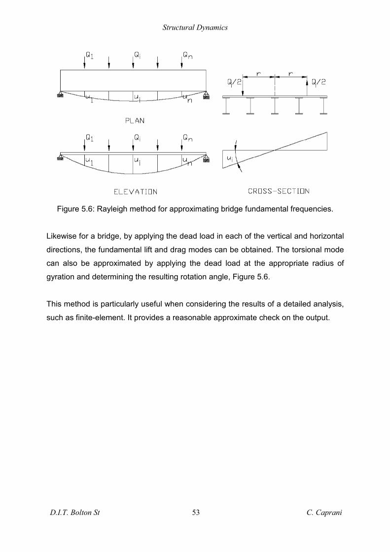
Figure 5.6: Rayleigh method for approximating bridge fundamental frequencies.

Likewise for a bridge, by applying the dead load in each of the vertical and horizontal

directions, the fundamental lift and drag modes can be obtained. The torsional mode

can also be approximated by applying the dead load at the appropriate radius of

gyration and determining the resulting rotation angle, Figure 5.6.

This method is particularly useful when considering the results of a detailed analysis,

such as finite-element. It provides a reasonable approximate check on the output.

Structural Dynamics


6. Appendix a. References

The following books/articles were referred to in the writing of these notes; particularly

Clough & Penzien (1993), Smith (1988) and Bolton (1978) - these should be referred

to first for more information. There is also a lot of information and software available

online; the software can especially help intuitive understanding. The class notes of

Mr. R. Mahony (D.I.T.) and Dr. P. Fanning (U.C.D.) were also used.

1. Archbold, P., (2002), “Modal Analysis of a GRP Cable-Stayed Bridge”,

Proceedings of the First Symposium of Bridge Engineering Research In

Ireland, Eds. C. McNally & S. Brady, University College Dublin.

2. Beards, C.F., (1983), Structural Vibration Analysis: modelling, analysis and

damping of vibrating structures, Ellis Horwood, Chichester, England.

3. Bhatt, P., (1999), Structures, Longman, Harlow, England.

4. Bolton, A., (1978), “Natural frequencies of structures for designers”, The

Structural Engineer, Vol. 56A, No. 9, pp. 245-253; Discussion: Vol. 57A, No. 6,

p.202, 1979.

5. Bolton, A., (1969), “The natural frequencies of continuous beams”, The

Structural Engineer, Vol. 47, No. 6, pp.233-240.

6. Case, J., Chilver, A.H. and Ross, C.T.F., (1999), Strength of Materials and

Structures, 4th edn., Arnold, London.

7. Clough, R.W. and Penzien, J., (1993), Dynamics of Structures, 2nd edn.,

McGraw-Hill, New York.

8. Cobb, F. (2004), Structural Engineer’s Pocket Book, Elsevier, Oxford.

9. Craig, R.R., (1981), Structural Dynamics – An introduction to computer

methods, Wiley, New York.

10. Ghali, A. and Neville, A.M., (1997), Structural Analysis – A unified classical

and matrix approach, 4th edn., E&FN Spon, London.

11. Irvine, M., (1986), Structural Dynamics for the Practising Engineer, Allen &

Unwin, London.

12. Kreyszig, E., (1993), Advanced Engineering Mathematics, 7th edn., Wiley.

13. Smith, J.W., (1988), Vibration of Structures – Applications in civil engineering

design, Chapman and Hall, London.

Structural Dynamics


b. Important Formulae

Section 2: SDOF Systems

Fundamental equation of motion ( ) ( ) ( ) ( )mu t cu t ku t F t+ + =

Equation of motion for free vibration 2( ) 2 ( ) ( ) 0u t u t u tξω ω+ + =

Relationship between frequency, circular frequency,

period, stiffness and mass: Fundamental frequency

for an SDOF system.

1 12 2

kfT m

ωπ π

= = =

Coefficient of damping 2 cm

ξω =

Circular frequency 2 km

ω =

Damping ratio cr

cc

ξ =

Critical value of damping 2 2crc m kmω= =

General solution for free-undamped vibration

( )( ) cosu t tρ ω θ= +

22 00 ;uuρ

ω = +

0

0

tan uu

θω

−=

Damped circular frequency, period and frequency

21dω ω ξ= −

2 ;dd

T πω

=2

ddf

ωπ

=

General solution for free-damped vibrations

( )( ) costdu t e tξωρ ω θ−= +

22 0 00 ;

d

u uu ξωρω

+= +

0 0

0

tand

u uu

ξωθω−

=

Logarithmic decrement of damping ln 2n

n m d

u mu

ωδ πξω+

= =

Half-amplitude method 0.11m

ξ ≅ when 0.5n m nu u+ =

Structural Dynamics


Amplitude after p-cycles 1

p

nn p n

n

uu uu+

+

=

Equation of motion for forced response (sinusoidal) 0( ) ( ) ( ) sinmu t cu t ku t F t+ + = Ω

General solution for forced-damped vibration

response and frequency ratio

( ) ( )sinpu t tρ θ= Ω −

( ) ( )1 22 220 1 2 ;F

kρ β ξβ

− = − +

2

2tan1ξβθβ

=−

βωΩ

=

Dynamic amplification factor (DAF) ( ) ( )1 22 22DAF 1 2D β ξβ

− ≡ = − +

Section 3: MDOF Systems

Fundamental equation of motion Mu + Cu + Ku = F

Equation of motion for undamped-free

vibration Mu + Ku = 0

General solution and derivates for free-

undamped vibration

( )sin tω φ+u = a

( )2 2sin tω ω φ ω− + = −u = a u

Frequency equation 2ω − K M a = 0

General solution for 2DOF system 1 1 1 2 2 1

2 2 2 2 2

0 00 0m u k k k u

m u k k u+ −

+ = −

Determinant of 2DOF system from

Cramer’s rule ( )2 2 2 2

2 1 1 2 2 2 0k k m k m kω ω ω − + − − − = K M =

Composite matrix 2ω = − E K M

Amplitude equation Ea = 0

Section 4: Continuous Structures

Equation of motion ( ) ( ) ( )4 2

4 2

, ,,

v x t v x tEI m p x t

x t∂ ∂

+ =∂ ∂

Assumed solution for free-undamped

vibrations ( ) ( ) ( ),v x t x Y tφ=

Structural Dynamics


General solution ( ) ( ) ( )

( ) ( )1 2

3 4

sin cos

sinh cosh

x A x A x

A x A x

φ α α

α α

= +

+ +

Boundary conditions for a simply

supported beam

( ) ( )2

20, 0 and 0, 0vv t EI tx∂

= =∂

( ) ( )2

2, 0 and , 0vv L t EI L tx∂

= =∂

Frequencies of a simply supported beam2

nn EIL mπω =

Mode shape or mode n: (A1 is normally

unity) ( ) 1 sinn

n xx ALπφ =

Cantilever beam boundary conditions ( ) ( )0, 0 and 0, 0vv t t

x∂

= =∂

( ) ( )2 3

2 3, 0 and , 0v vEI L t EI L tx x∂ ∂

= =∂ ∂

Frequency equation for a cantilever cos( )cosh( ) 1 0L Lα α + =

Cantilever mode shapes ( )

( )

1

sin( ) sinh( )sin( ) sinh( )cos( ) cosh( )

cosh( ) cos( )

n

x xL Lx AL L

x x

α αα αφα α

α α

− +

+ = × +

−

Bolton method general equation 1

2E

E

KfMπ

=

Section 5: Practical Design

Peak acceleration under foot-loading ( )0 0.9 2 Ia f

Mπ=

70 NsI ≈ 40% mass per unit areaM ≈

Maximum dynamic deflection max stu u Kψ=

Maximum vertical acceleration 2max maxu uω=

BD37/01 requirement for vertical acceleration 0.5 f±

Structural Dynamics


Var

iatio

nof

DA

Fw

ithda

mpi

ngan

dfre

quen

cyra

tios

c.Im

port

antT

able

san

dFi

gure

s

Sect

ion

2:SD

OF

Syst

ems

Und

ampe

dfre

e-vi

brat

ion

resp

onse

Gen

eral

case

ofan

unde

r-crit

ical

lyda

mpe

dsy

stem

Structural Dynamics


Bol

ton’

sta

ble

Sect

ion

4:C

ontin

uous

Stru

ctur

es

Firs

tthr

eem

odes

fora

ns-

sbe

aman

dca

ntile

ver

Equ

ival

entd

ynam

icm

ass

dist

ribut

ions

Structural Dynamics


Rec

omm

ende

dvi

brat

ion

limits

forl

ight

floor

s.

Sect

ion

5:Pr

actic

alD

esig

n

Equ

alse

nsat

ion

cont

ours

forv

ertic

alvi

brat

ion

Structural Dynamics


Dyn

amic

resp

onse

fact

orfo

rfoo

tbrid

ges

Sect

ion

5:Pr

actic

alD

esig

n

Con

figur

atio

nfa

ctor

sfo

rfoo

tbrid

ges.

structural dynamics final year - structural engineering bsc

Documents