structural break threshold vars for predicting us recessions using the spread

Structural Break Threshold VARs for Predicting US Recessions Using the SpreadAuthor(s): Ana Beatriz C. GalvãoSource: Journal of Applied Econometrics, Vol. 21, No. 4 (May - Jun., 2006), pp. 463-487Published by: WileyStable URL: http://www.jstor.org/stable/25146440 .

Accessed: 16/12/2014 04:15

Your use of the JSTOR archive indicates your acceptance of the Terms & Conditions of Use, available at .http://www.jstor.org/page/info/about/policies/terms.jsp

.JSTOR is a not-for-profit service that helps scholars, researchers, and students discover, use, and build upon a wide range ofcontent in a trusted digital archive. We use information technology and tools to increase productivity and facilitate new formsof scholarship. For more information about JSTOR, please contact [email protected].

.

Wiley is collaborating with JSTOR to digitize, preserve and extend access to Journal of Applied Econometrics.

http://www.jstor.org

This content downloaded from 138.73.1.36 on Tue, 16 Dec 2014 04:15:50 AMAll use subject to JSTOR Terms and Conditions

http://www.jstor.org/action/showPublisher?publisherCode=black

http://www.jstor.org/stable/25146440?origin=JSTOR-pdf

http://www.jstor.org/page/info/about/policies/terms.jsp


JOURNAL OF APPLIED ECONOMETRICS J. Appl. Econ. 21: 463-487 (2006) Published online in Wiley InterScience (www.interscience.wiley.com). DOI: 10.1002/jae.840

STRUCTURAL BREAK THRESHOLD VARs FOR PREDICTING US RECESSIONS USING THE SPREAD

ANA BEATRIZ C. GALVAO*

Ibmec Sao Paulo, Rua Maestro Cardim 1170, Sao Paulo SP 01323001, Brazil

SUMMARY

This paper proposes a model to predict recessions that accounts for non-linearity and a structural break

when the spread between long- and short-term interest rates is the leading indicator. Estimation and model

selection procedures allow us to estimate and identify time-varying non-linearity in a VAR. The structural

break threshold VAR (SBTVAR) predicts better the timing of recessions than models with constant threshold or with only a break. Using real-time data, the SBTVAR with spread as leading indicator is able to anticipate

correctly the timing of the 2001 recession. Copyright ? 2006 John Wiley & Sons, Ltd.

1. INTRODUCTION

Economic forecasters do not usually enjoy a good reputation when trying to predict a possible US recession: 'the dismal scientists have a dismal record in predicting recessions' iThe Economist,

2001). The problem is that recessions are relatively rare events with potentially strong negative consequences for individuals as well as businesses. The main contribution of this paper is to

propose a model to predict recessions that accounts for non-linearity and a structural break when

the spread between long- and short-term interest rates is the leading indicator. Estimation and model selection procedures allow us to estimate and identify time-varying non-linearity in a VAR. The model with time-varying thresholds predicts better the timing of recessions than models with constant threshold or with only a break.

The literature presents evidence that the spread, which represents the term structure of interest

rates, is a reliable predictor of output growth (Estrella and Hardouvelis, 1991; Hamilton and Kim, 2002; Berk, 1998; Stock and Watson, 2001). The information contained in the spread reflects not

only monetary policy but future expected short rates and changes in the risk premium (Hamilton and Kim, 2002). In fact, the spread keeps its predictive power when other indicators of monetary

policy (Anderson and Vahid, 2001) and oil prices (Hamilton and Kim, 2002) are included in a

regression to explain output growth. The spread is also a reliable predictor of the probability of recession (Lahiri and Wang, 1996; Estrella and Mishkin, 1998).

However, Haubrich and Dombrosky (1996), Dotsey (1998) and Stock and Watson (2001) report that the predictive power of the spread between long- and short-term interest rates has decreased after 1985. The failure of the indicator index of Stock and Watson (1989) to predict the 1990-91 recession has been attributed to the fact that the index relied heavily on the spread (Dotsey, 1998). In contrast, employing Markov-switching models to obtain the probability of recession, Lahiri and

Wang (1996) showed that the spread managed to predict the last recession. Likewise, Duecker

* Correspondence to: Ana Beatriz C. Galvao, Ibmec Sao Paulo, Rua Maestro Cardim 1170, Paraiso, 01323-001 Sao

Paulo, Brazil. E-mail: [email protected]

Copyright ? 2006 John Wiley & Sons, Ltd. Received 14 April 2003

Revised 7 October 2004



464 A. B. C GALVAO

(1997) and Estrella and Mishkin (1998), using probit, demonstrate that the spread is still better

than other leading indicators in predicting recessions for the USA. The tests presented by Estrella

et al. (2003) support the view that while there is no instability in the ability of the spread to predict recessions, the ability of the spread to predict economic growth is unstable. Recently, Chauvet

and Potter (2002) questioned these results with findings of parameter instability in probit models.

The literature also presents evidence of non-linearities in models that use the spread to predict

output growth (Galbraith and Tkacz, 2000; Anderson and Vahid, 2001). The inclusion of non

linearities improves the accuracy of predicting the probability of recession (Anderson and Vahid,

2001), while large spreads do not predict strong growth (Galbraith and Tkacz, 2000).

Regarding changes in the output growth series, an important stylized fact is that the variability of output growth decreased after 1984 (Kim and Nelson, 1999; McConnell and Perez-Quiros,

2000). Regarding interest rates, Watson (1999) suggests that the variability of the US long-term interest rate has been increasing while the short-term interest rate is smoothed by the monetary

authority. However, the results of the tests applied by Sensier and Van Dijk (2001) indicate that

while there is evidence of structural breaks in short- and long-term interest rates, the evidence of

a structural break in their spread is not strong. Therefore, the literature suggests that a linear model between output growth and spread is not

a proper representation of the dynamic responses between these variables because of parameter

instability (Estrella et al., 2003; Stock and Watson, 2001), non-linearities (Galbraith and Tkacz,

2000; Anderson and Vahid, 2001) and changes in the variability of the output growth (Kim and

Nelson, 1999; McConnell and Perez-Quiros, 2000). The structural break threshold VAR (SBTVAR)

proposed in this paper is able to account for these characteristics and can be employed to generate more precise predictions of recessions.

This paper extends some previous results published in the literature in two issues. Structural

breaks are necessary to time correctly direction-of-change predictions not only in linear (Pesaran and Timmermann, 2004) but also in non-linear models. The spread leads the 2001 recession (Stock and Watson, 2003) but the model with threshold and structural breaks is more efficient in extracting the information from the spread than a simple VAR is.

The remainder of this paper is organized as follows. Structural break threshold VARs are

presented in Section 2, which also includes estimation and specification procedures. In addition, the

SBTVAR is applied to model the output growth and the spread, and the estimates are compared with

more restrictive specifications. Section 3 presents the definitions of recession and the loss function

employed to evaluate forecasting performance. The evaluation of the in-sample and real-time

performance in event forecasting of VARs, threshold VARs, structural break VARs and SBTVARs

is also presented in Section 3. Section 4 analyses real-time forecasts for the 2001 recession and

compares the results obtained with other forecast evaluations presented in the literature. Section

5 summarizes the main findings of this paper and concludes.

2. STRUCTURAL BREAK THRESHOLD VARS

Threshold VARs are piecewise linear models with different autoregressive matrices in each regime, determined by a transition variable (one of the endogenous variables), a delay and a threshold (Tsay,

1998). Structural break models also divide the sample into two regimes but they are determined

by a break-point and are not recurrent, allowing different dynamics before and after the break.

Although non-linear models can capture some characteristics of structural break models (Koop

Copyright ? 2006 John Wiley & Sons, Ltd. J. Appl. Econ. 21: 463-487 (2006)



STRUCTURAL BREAK THRESHOLD VARs 465

and Potter, 2000, 2001; Carrasco, 2002), it may be the case that the break also implies changes in

the parameters that determine the non-linearity. Univariate time-varying smooth transition models

have been proposed by Lundbergh et al. (2003) and have been applied to capture changes in

seasonality of industrial production by Van Dijk et al. (2003). In this section, a VAR with threshold

non-linearity and a structural break is proposed. In contrast with time-varying smooth transition

models, structural break threshold models characterize abrupt changes from one regime to another.

After discussing how to estimate and verify whether there are thresholds and breaks in the data,

the model is applied to US output growth and spread. The robustness of the estimates of the

empirical exercise is verified by observing recursive estimates based on real-time data.

Define xt as a m x 1 vector of m endogenous variables xt =

ix\t, x2t,..., xmt)' and define the

m x imp + 1) matrix xt-\ = (1, xt-\, ,xt-p) where p is the autoregressive order. A structural

break threshold VAR can then be written as:

xf = {[fe_1A)/i,^1(n) + te-i^2)(l-/i,^1(ri))]/,(r)}+

{[ixt-xfo)htt-d2ir2) + Oc-i&Xl -

l2j-d2(r2))]H - I tit))} + k,

where //^^(r,) is an indicator function that depends on a transition variable z, on a threshold r,

and on a delay d^. /^-^(r,-) = 1 izt-dt

< n) and Itix) is an indicator function that depends on a

break-point r: /r(r) = 1 (r < r). pi are imp + l)xm matrices of parameters. ut is the m x 1 vector

of disturbances that is assumed to have a mean equal to zero and a constant m x m covariance

matrix E. This supposition is easily substituted by constant variance conditional on the regime. The SBTVAR has one threshold VAR (TVAR) in each subsample determined by the break-point.

This means that the break affects also the parameters of the indicator functions that determine

the regimes. Although it is possible to write a nested specification using logistic functions, the smoothness analogy estimated by Lundbergh et al. (2003) does not consider changes in the

transition function following the break. Allowing the restriction that r\ = r2, given that d\ ?

d2, the parameters of the dynamics are allowed to change in each subsample but not the parameters of the regime-switching function. The model with this restriction is called SBTVARc. If there is

no threshold given that there is a break-point, a structural break VAR is written as:

xt = ixt-iPi)Itir) + fe-i&Xl -

IM) + ut

In contrast, if there is a threshold but no structural break, one has a threshold VAR:

xt = ixt-iPi)It-dir) + (*,-iA)(l -

h-dir)) + ut

Finally, if there is no break or threshold, the last two specifications are simplified to a VAR.

2.1. Conditional Means Based on Simulated DGPs (Data Generating Process)

An interesting application of time-varying and threshold VARs is to capture changes in the

predictive power of a variable x2t on another variable x\t. In this subsection, data from nested

but different DGPs are simulated to observe the implications of a TVAR, SB VAR, SBTVARc and

SBTVAR on the conditional mean Eix\t\x2t-\). The DGPs are described in Table I. x2t causes

(Granger sense) x\t in the lower regime of the TVAR, and in the first subsample of the SB VAR.

This causality is also present in the lower regime of the first subsample of the SBTVARc and




466 A. B. C GALVAO

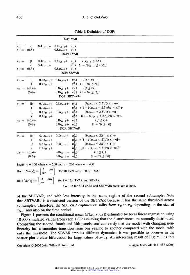
Table I. Definition of DGPs

DGP: VAR

xu = ( 0.4xif _i 4- 0.8x2,_i + uu)

x2t = (0.5+ 0.8*2.-1+ u2t)

DGP: TVAR

xu = {( 0.4xi._i+- 0.8x2,_i + u\t) I(x2t-i < 2.5)+

( 0.4jcif_i+ u\t) (l-/(x2,-i <2.5))}

x2, = (0.5+ 0.8*2.-1+ ?2f)

DGP: SBVAR

xi, = {( 0.4xi,_i+ 0.8x2,-1+ u\t) /(r<r)+

( 0.4xi,_i+ ??,) (1-/(/<t))} *2r =

{(0.4+ 0.8x2,-1+ u\t) I(t < r)+

(0.6+ 0.8x2,-1+ u\t) (l-/(r<r))}

DGP: SBTVARc

xi, = {[( 0.4xi,_i+ 0.8x2,-1+ u\t) (/(x2,_i

< 2.5)/(f < r))+

( 0.4xi,_i+ ?2f) ((1 -

/(x2,-i < 2.5))/(f < r))]+

[( 0.4xi,_i+ 0.3x2,-i+ u\t) (/(x2,-i < 2.5)/(r > r))+

( 0.4xi,_i+ u\t) ((1 -

/(X2,_i < 2.5))/(. > t))].

x2t= {(0.4+ 0.8x2,-1+ u\t) I(t<r)+

(0.6+ 0.8x2,-1+ u\t) (l-I(t <r))}

DGP: SBTVAR

xi, = {[( 0.4xi,_i+ 0.8x2,-1+ ?lr) (/(x2,-i < 2)I(t < r))+

( 0.4xi,_i+ 4) ((1 -

7(x2,-i < 2))/(. < r))]+

[( 0.4xi,_i+ 0.3x2,-1+ 4) (7(x2,-i < 3)/(r > r))+

( 0.4xi,_i+ u\t) ((1 -

/(x2,-i < 3))/(. > r))]}.

x2, = {(0.4+ 0.8x2,_i+ u\t) I(t<r)+

(0.6+ 0.8x2,-1+ 4) (l-/(f<r))}

Break: t = 100 when n = 200 and t = 200 when n = 400.

Horn.: Var(?i) = ! c?r for all i;car = 0, -0.3, -0.6 v t;

[cor 1 J

Het.: Var(Mj) = |

3 C^V | for i = lfor TVAR and SBVAR v f/

[cov 1 J i = 1, 2 for SBTVARc and SBTVAR; same cor as horn.

of the SBTVAR, and with less intensity in this same regime of the second subsample. Note

that SBTVARc is a restricted version of the SBTVAR because it has the same threshold across

subsamples. Therefore, the SBTVAR captures causality from X2t to x\t depending on the size of

X2t-\ and also on the time period.

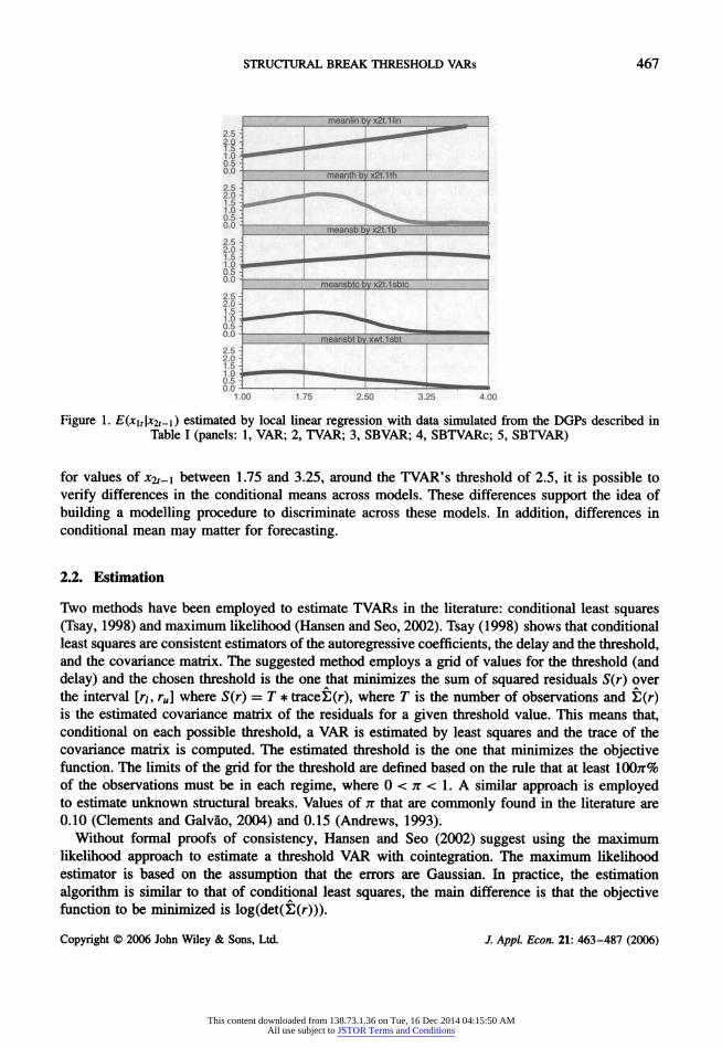
Figure 1 presents the conditional mean (?(*2f |Jtir_i)) estimated by local linear regression using

10000 simulated values from each DGP assuming that the disturbances are normally distributed.

Comparing the second, fourth and fifth panels, one can verify that the model with changing non

linearity has a smoother transition from one regime to another compared with the model with

only the threshold. The SBVAR implies different dynamics: it was possible to observe in the

scatter plot a clear bifurcation for large values of Jt2r-i. An interesting result of Figure 1 is that

Copyright ? 2006 John Wiley & Sons, Ltd. J Appl. Econ. 21: 463-487 (2006)




2.5: __^^*__--* ^^^^^

0;0: ___________________^ ____________________________________________________________

0.5 ? ^^. ___________________

o!o - ^^^^_ ^^^^_ ^^^^^ ^^^^_

?] _^

2.5

?_:_

0.0 J- -'-.-1 _^?^^--___. 1.00 1.75 2.50 3.25 4.00

Figure 1. E(x\t\x2t-i) estimated by local linear regression with data simulated from the DGPs described in Table I (panels: 1, VAR; 2, TVAR; 3, SBVAR; 4, SBTVARc; 5, SBTVAR)

for values of X2t-\ between 1.75 and 3.25, around the TVAR's threshold of 2.5, it is possible to

verify differences in the conditional means across models. These differences support the idea of

building a modelling procedure to discriminate across these models. In addition, differences in

conditional mean may matter for forecasting.

2.2. Estimation

Two methods have been employed to estimate TVARs in the literature: conditional least squares

(Tsay, 1998) and maximum likelihood (Hansen and Seo, 2002). Tsay (1998) shows that conditional least squares are consistent estimators of the autoregressive coefficients, the delay and the threshold, and the covariance matrix. The suggested method employs a grid of values for the threshold (and

delay) and the chosen threshold is the one that minimizes the sum of squared residuals S(r) over

the interval [r/, ru] where S(r) = T * trace _t_(r), where T is the number of observations and ?(r) is the estimated covariance matrix of the residuals for a given threshold value. This means that, conditional on each possible threshold, a VAR is estimated by least squares and the trace of the covariance matrix is computed. The estimated threshold is the one that minimizes the objective function. The limits of the grid for the threshold are defined based on the rule that at least 100;r% of the observations must be in each regime, where 0 < n < 1. A similar approach is employed to estimate unknown structural breaks. Values of tx that are commonly found in the literature are

0.10 (Clements and Galvao, 2004) and 0.15 (Andrews, 1993). Without formal proofs of consistency, Hansen and Seo (2002) suggest using the maximum

likelihood approach to estimate a threshold VAR with cointegration. The maximum likelihood

estimator is based on the assumption that the errors are Gaussian. In practice, the estimation

algorithm is similar to that of conditional least squares, the main difference is that the objective function to be minimized is log(det(?(r))).

Copyright ? 2006 John Wiley & Sons, Ltd. /. Appl. Econ. 21: 463-487 (2006)



468 A. B. C. GALVAO

Both approaches can be employed to estimate the SBTVAR. Supposing that the delays, the

autoregressive order and the transition variable are known, the matrices ^1,^2,^3,^4 can be obtained

by ordinary least squares (OLS) given values of r\,r2 and x. This means that one can concentrate the residual sum of squared errors and the likelihood function with respect to the thresholds and the

break-point. Grids of possible values of thresholds and break-point can be defined supposing that at least 1007T% of the observations are available to estimate the autoregressive coefficients in each

regime. For each possible combination of values inside the grids, one can compute P\,P2,P3,p4 by OLS. Based on these estimates, the residuals ut can be obtained and saved in the T x m matrix u. Using the residuals, the covariance matrix is consistently computed as E(ri, r2,x) =

iuru)/T. The estimator of conditional least squares (CLS) is obtained by:

ru h, i = ng ru T * trace(E(ri, r2, x)) q<r2<ru t/<T<TU

Similarly, the estimator of maximum likelihood (ML) is obtained by:

h,r2, r= r/jnjnrM log(det(X](ri,r2,T))) ri<r2<ru T/<r<rM

The maximum likelihood estimator is built assuming that the covariance matrices are the same for each regime. This assumption may not hold when applied to macroeconomic data with

time-varying variances, but the estimator can be modified to allow regime-switching variances. SBTVAR has four regimes (two regimes in each subsample), so that the conditional variance matrix

S/(ri, r2, x) is computed with the Ti observations of ut of regime /. The maximum likelihood

estimator that allows changes in the regime-dependent variances (HML) is written as:

... /^log(det(t1(r1,r2,r))) + ̂ log(det(i:2(r1,r2,r)))+\ /*i ? f2, X = mm I Tp Tp I

'IpF V Y log(det(?3(rlt r2, r))) + %f log(det(S4(r,, r2, t))) /

Similarly, CLS, ML and HML estimators can be derived to estimate SBTVARc, SBVAR and TVAR. The comparative unbiasedness and efficiency in finite samples of those three estimators are investigated using a Monte Carlo exercise.

The properties of the CLS, ML and HML are evaluated for two sample sizes: T = 200 and T = 400. The size of the sample in the empirical part is around 200. In addition, different

suppositions about the variance matrix of the disturbances are made: constant variance and variance

changing with regimes; disturbances independent across equations or with some correlation. The

DGPs are the same as employed in the last section, described in Table I.

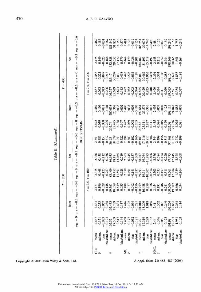
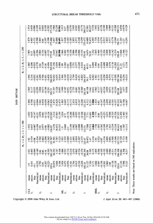
Table II presents the mean of the estimates, their standard errors and average bias for each

assumption on the covariance matrix, for each estimation method and for each DGP with 500

replications. The estimators are computed conditional on having at least 15% of the observations

in each regime and at least 30% of the observations in each subsample. The results show bias in

the estimation of the break-point x of the SBTVAR using CLS and ML when the disturbances'

variance changes across regimes. Therefore, if there is any suspicion of possible changes in the

variance across regimes in the SBTVAR, the HML is recommended. In the remainder of this

paper, all the specifications (except VAR) are estimated using the HML.




o o

|- Table II. Performance of estimation procedures for TVAR, SBVAR, SBTVARc and SBTVAR

cr _

? 7 = 200 7 = 400

to - -

?> horn het horn het

?r o\2 = 0 an = ?0.3 an = ?0.6 ai2 =0 <7i2 = ?0.3 o\2 ? ?0.6 o\2 = 0 cri2 = ?0.3 ai2 = ?0.6 (J12 =0 o\2 ? ?0.3 o\2 = ?0.6 ^ DGP: TVAR

% r = 2.5 r = 2.5

fc> _

o CLS mean 2.495 2.486 2.494 2.449 2.453 2.434 2.499 2.499 2.498 2.485 2.484 2.488 5 r std.err. 0.056 0.049 0.045 0.143 0.157 0.245 0.023 0.024 0.026 0.041 0.047 0.056 % r bias -0.005 -0.014 -0.006 -0.051 -0.047 -0.066 -0.001 -0.001 -0.002 -0.015 -0.016 -0.012 2

P* bias/std.err. -0.089 -0.286 -0.133 -0.357 -0.299 -0.269 -0.043 -0.042 -0.077 -0.366 -0.340 -0.214 o ML mean 2.494 2.489 2.495 2.437 2.459 2.47 2.5 2.498 2.5 2.484 2.486 2.494 g

r std.err. 0.049 0.045 0.032 0.172 0.115 0.115 0.02 0.025 0.021 0.041 0.043 0.033 g

bias -0.006 -0.011 -0.005 -0.063 -0.041 -0.03 0 -0.002 0 -0.016 -0.014 -0.006 P bias/std.err. -0.122 -0.244 -0.156 -0.366 -0.357 -0.261 0.000 -0.080 0.000 -0.390 -0.326 -0.182 ?

HML mean 2.492 2.486 2.494 2.483 2.481 2.491 2.498 2.498 2.501 2.497 2.496 2.502 g r std.err. 0.049 0.057 0.032 0.061 0.064 0.046 0.023 0.025 0.021 0.032 0.031 0.029 >

bias -0.008 -0.014 -0.006 -0.017 -0.019 -0.009 -0.002 -0.002 0.001 -0.003 -0.004 0.002 ^

bias/std.err. -0.163 -0.246 -0.188 -0.279 -0.297 -0.196 -0.087 -0.080 0.048 -0.094 -0.129 0.069 X

DGP: SBVAR S

_ _ _ C/3

-?- ?H

r = 100 r = 200 O

r"

- O

CLS mean 99.532 99.672 99.798 97.985 98.447 99.133 199.11 199.448 200.036 197.59 198.594 199.504 <

r std.err. 3.993 3.592 4.096 5.328 4.892 4.999 2.207 2.2 3.014 5.138 3.499 3.458 %

bias -0.468 -0.328 -0.202 -2.015 -1.553 -0.867 -0.888 -0.552 0.036 -2.414 -1.406 -0.496

s bias/std.err. -0.228 -0.259 -0.448 -0.363 -0.449 -0.594 -0.407 -0.354 -0.310 -0.497 -0.458 -0.517

^ ML mean 99.532 99.161 98.951 98.272 97.908 97.852 199.13 199.21 199.308 197.8 198.132 198.65

^ t std.err. 4.018 3.351 2.363 5.344 5.524 3.889 2.233 2.062 1.748 5.54 3.621 2.691

t*i bias -0.468 -0.839 -1.049 -1.728 -2.092 -2.148 -0.874 -0.79 -0.692 -2.204 -1.868 -1.35

? bias/std.err. -0.228 -0.259 -0.448 -0.363 -0.449 -0.594 -0.407 -0.354 -0.310 -0.497 -0.458 -0.517

^ HML mean 99.217 99.161 98.86 98.902 98.58 98.587 199.1 199.238 199.364 198.86 198.888 198.958

^ t std.err. 3.438 3.244 2.546 3.028 3.16 2.377 2.217 2.152 2.05 2.293 2.428 2.014

6 bias -0.783 -0.839 -1.14 -1.098 -1.42 -1.413 -0.902 -0.762 -0.636 -1.14 -1.112 -1.042

Y bias/std.err. -0.228 -0.259 -0.448 -0.363 -0.449 -0.594 -0.407 -0.354 -0.310 -0.497 -0.458 -0.517

^_ _ oo ?

^ (continued overleaf)



^3 r-_

P. ? to o

.g Table II. (Continued).

fr -

c/_ r = 200 r = 400

o _ _

S3

horn het horn het

r

^* CTi2 = 0 CTi2 = ?0.3 0\2 = ?0.6 <7i2 = 0 <Ti2 = ?0.3 0\2 = ?0.6 <Ti2 = 0 <Ti2 = ?0.3 <7i2 = ?0.6 <Ti2 = 0 C712 = ?0.3 0*12 = ?0.6 DGP: SBTVARc

r = 2.5, t = 100 r = 2.5, r = 200 >

_ W

CLS mean 2.467 2.433 2.471 2.375 2.388 2.35 2.492 2.489 2.487 2.453 2.475 2.469 P f std.err. 0.171 0.233 0.196 0.468 0.438 0.481 0.039 0.106 0.063 0.221 0.149 0.186 O

bias -0.033 -0.067 -0.029 -0.125 -0.112 -0.15 -0.008 -0.011 -0.013 -0.047 -0.025 -0.031 ?

bias/std.err. -0.193 -0.288 -0.148 -0.267 -0.256 -0.312 -0.205 -0.104 -0.206 -0.213 -0.168 -0.167 <

z mean 102.52 102.433 99.361 88.409 86.935 86.95 202.74 200.038 196.327 186.17 182.828 181.847 g'

std.err. 17.509 17.789 18.059 18.452 18.18 18.079 25.475 23.368 25.629 30.207 29.652 31.824 bias 2.517 2.433 -0.639 -11.591 -13.065 -13.05

2.738 0.038 -3.673 -13.83 -17.172 -18.153

bias/std.err. 0.144 0.137 -0.035 -0.628 -0.719 -0.722 0.107 0.002 -0.143 -0.458 -0.579 -0.570

ML mean 2.468 2.446 2.488 2.359 2.363 2.398 2.492 2.496 2.497 2.445 2.464 2.481 r std.err. 0.177 0.192 0.077 0.491 0.445 0.383 0.039 0.038 0.032 0.276 0.179 0.123

bias -0.032 -0.054 -0.012 -0.141 -0.137 -0.102 -0.008 -0.004 -0.003 -0.055 -0.036 -0.019

^ bias/std.err. -0.181 -0.281 -0.156 -0.287 -0.308 -0.266 -0.205 -0.105 -0.094 -0.199 -0.201 -0.154

? r mean 102.29 101.018 100.259 89.293 88.017 89.183 202.83 199.684 200.825 185.04 184.482 185.254 ^ std.err. 17.319 18.209 16.488 19.31 19.764 17.916 25.511 23.574 20.429 30.462 31.193 30.078

? bias 2.289 1.018 0.259 -10.707 -11.983 -10.817 2.827 -0.316 0.825 -14.965 -15.518 -14.746

? bias/std.err. 0.132 0.056 0.016 -0.554 -0.606 -0.604 0.111 -0.013 0.040 -0.491 -0.497 -0.490

k> HML mean 2.44 2.41 2.454 2.303 2.376 2.344 2.485 2.493 2.499 2.394 2.448 2.48

- r std.err. 0.346 0.362 0.191 0.633 0.584 0.499 0.084 0.057 0.034 0.374 0.213 0.126

& bias -0.06 -0.09 -0.046 -0.197 -0.124

-0.156

-0.015 -0.007 -0.001 -0.106 -0.052 -0.02

V bias/std.err. -0.173 -0.249 -0.241 -0.311 -0.220 -0.313 -0.179 -0.123 -0.029 -0.283 -0.244 -0.159

? t mean 101.98 102.264 100.666 98.661 97.475 97.768 202.08 198.115 199.615 198.15 198.349 198.245

^ std.err. 19.293 19.861 19.309 12.884 12.145 11.221 25.756 24.843 22.59 9.696 10.065 7.155

g bias 1.981 2.264 0.666 -1.339 -2.525 -2.232 2.075 -1.885 -0.385 -1.855 -1.651 -1.755

S bias/std.err. 0.103 0.114 0.034 -0.104 -0.208 -0.199 0.081 -0.076 -0.017 -0.191 -0.164 -0.245



n

>% DGP: SBTVAR

2. _ OQ

5* R\ = 2, R2 = 3, t = 100 /?i = 2, R2 = 3, t = 200

@ -

g CLS mean 1.9 1.931 1.92 1.933 1.853 1.969 1.965 1.948 1.965 1.903 1.879 1.914

8 h std.err. 0.431 0.493 0.519 0.647 0.635 0.708 0.117 0.216 0.206 0.33 0.403 0.458

S bias -0.1 -0.069 -0.08 -0.067 -0.147 -0.031 -0.035 -0.052 -0.035 -0.097 -0.121 -0.086

?* bias/std.err. -0.232 -0.140 -0.154 -0.104 -0.231 -0.044 -0.299 -0.241 -0.170 -0.294 -0.300 -0.188

^ r2 mean 2.793 2.66 2.702 2.92 2.878 2.941 2.804 2.699 2.64 2.903 2.803 2.815 Sr std.err. 0.93 0.86 0.863 0.977 0.981 0.939 0.673 0.706 0.729 0.734 0.64 0.655

^ bias -0.207 -0.34 -0.298 -0.08 -0.122 -0.059 -0.196 -0.301 -0.36 -0.097 -0.197 -0.185

? bias/std.err. -0.223 -0.395 -0.345 -0.082 -0.124 -0.063 -0.291 -0.426 -0.494 -0.132 -0.308 -0.282

g t mean 105.6 103.147 103.787 136.07 135.993 135.829 205.33 200.835 205.039 275.95 275.668 275.239 std.err. 29.875 30.252 30.391 2.479 3.214 2.872 57.397 59.052 57.256 2.619 3.657 3.968 H ? bias 5.604 3.147 3.787 36.072 35.993 35.829 5.328 0.835 5.039 75.947 75.668 75.239 {2

bias/std.err. 0.188 0.104 0.125 14.551 11.199 12.475 0.093 0.014 0.088 28.998 20.691 18.961 Q

ML mean 1.924 1.886 1.951 1.9 1.824 1.885 1.949 1.966 1.99 1.864 1.837 1.915 3 h std.err. 0.473 0.522 0.325 0.669 0.71 0.665 0.185 0.109 0.202 0.402 0.426 0.37 g

bias -0.076 -0.114 -0.049 -0.1 -0.176 -0.115 -0.051 -0.034 -0.01 -0.136 -0.163 -0.085 r

bias/std.err. -0.161 -0.218 -0.151 -0.149 -0.248 -0.173 -0.276 -0.312 -0.050 -0.338 -0.383 -0.230 g

r2 mean 2.764 2.676 2.693 2.902 2.899 2.833 2.755 2.749 2.751 2.906 2.852 2.905 g std.err. 0.915 0.862 0.819 0.987 0.955 0.835 0.681 0.624 0.577 0.709 0.571 0.547 ? bias -0.236 -0.324 -0.307 -0.098 -0.101 -0.167 -0.245 -0.251 -0.249 -0.094 -0.148 -0.095 H

bias/std.err. -0.258 -0.376 -0.375 -0.099 -0.106 -0.200 -0.360 -0.402 -0.432 -0.133 -0.259 -0.174 K

r mean 105.33 105.395 103.47 133.51 133.601 132.251 201.84 204.835 204.9 270.93 270.472 269.237 ? std.err. 31.127 30.88 29.972 7.508 7.711 8.312 60.108 59.3 49.53 9.674 10.689 12.981 g bias 5.326 5.395 3.47 33.512 33.601 32.251 1.841 4.835 4.9 70.93 70.472 69.237 O

bias/std.err. 0.171 0.175 0.116 4.464 4.358 3.880 0.031 0.082 0.099 7.332 6.593 5.334 5

HML mean 1.844 1.895 1.93 1.738 1.775 1.833 1.963 1.961 1.984 1.845 1.726 1.842 < h std.err. 0.597 0.546 0.522 1.053 0.89 0.82 0.117 0.131 0.04 0.464 0.534 0.453 g

bias -0.156 -0.105 -0.07 -0.262 -0.225 -0.167 -0.037 -0.039 -0.016 -0.155 -0.274 -0.158

5 bias/std.err. -0.261 -0.192 -0.134 -0.249 -0.253 -0.204 -0.316 -0.298 -0.400 -0.334 -0.513 -0.349

? h mean 2.862 2.689 2.695 2.781 2.675 2.699 2.859 2.828 2.864 2.858 2.822 2.869 ?. std.err. 1.08 0.984 0.881 1.013 0.996 0.842 0.671 0.574 0.478 0.648 0.517 0.489

t*i bias -0.138 -0.311 -0.305 -0.219 -0.325

-0.301

-0.141 -0.172 -0.136 -0.142 -0.178 -0.131

? bias/std.err. -0.128 -0.316 -0.346 -0.216 -0.326 -0.357 -0.210 -0.300 -0.285 -0.219 -0.344 -0.268

^ t mean 102.6 104.308 103.733 98.413 97.535 99.232 201.68 199.744 203.271 198.45 196.73 199.121

~ std.err. 21.132 19.841 18.729 14.08 13.459 11.497 30.027 25.854 21.22 12.604 11.241 6.836

6 bias 2.596 4.308 3.733 -1.587 -2.465 -0.768 1.677 -0.256 3.271 -1.546 -3.27 -0.879

f bias/std.err. 0.123 0.217 0.199 -0.113 -0.183 -0.067 0.056 -0.010 0.154 -0.123 -0.291 -0.129

-&> _ oo -

o

c$ Note: These results are based on 500 replications.



472 A. B. C. GALVAO

2.3. Choosing Between VAR, TVAR, SBVAR, SBTVARc and SBTVAR

Even if one can estimate SBTVARs, it is not clear whether it is necessary to have time-varying thresholds to capture the dynamic structure of the data. Tests for a threshold in a SBVAR or

for a break-point in a TVAR are complicated because of the discontinuity of the changes and the presence of nuisance parameters. The non-standard distributions of the supLM and sup Wald statistics for testing for unknown breaks and thresholds have been derived, respectively, by

Andrews (1993) and Hansen (1996). In this paper, a convenient specification method is proposed based on the asymptotic bounds for LM and Wald tests derived by Altissimo and Corradi (2002). The authors show how to compute bounds based on the law of the iterated logarithm such that a

decision rule is built for the rejection of the null. Altissimo and Corradi show that the decision rule is effective to choose correctly between a linear and a threshold model. In this section, selection criteria based on the bounds of supLM and sup Wald statistics are employed to discriminate between

VAR, TVAR, SBVAR, SBTVARc and SBTVAR in a specific-to-general approach. The ability of this approach to discriminate between VAR specifications in finite samples is evaluated with a

simulation exercise.

The decision rule for model selection employed in this paper uses asymptotic bounds

(l/21n(ln(_T))) and the maximum value of a Wald and LM statistic over a grid of possible values for

the nuisance parameter as proposed by Altissimo and Corradi (2002). The Wald and LM statistics are computed using the sum of squared residuals (SSR) under the null and the alternative:

u >_ (SSR(0x) -

SSR(02)\ (SSR&Q -

SSR(02)\ W(02)

= n - ; LM(02)

= n -..

^ SSR(02) J \ sSRm J The vector 6\ has parameters such as thresholds and breaks of the model under the null and 02 has those parameters of the models under the alternative. The rule that ensures that type I and

type II errors are asymptotically zero is that the model under the alternative must be chosen if the

bounded ^\xVeL<92<eu W(??2) (or sup^<^<ei/ LM(02)) is larger than one. Specifically:

. i r ri choose model under alternative if BWald = ??- sup W(02) > 1

21n(ln(r)) L^<fc<02" J

Similarly, the rule can also be written employing the sup^^^t/ LM(02) statistic.

Based on the results of Lundbergh et al. (2003) that a specific-to-general approach can specify carefully time-varying smooth transition models, a specific-to-general approach based on the

asymptotic decision rules is employed to choose between a VAR, a TVAR, a SBVAR, a SBTVARc

and a SBTVAR. In this model selection procedure, delays, transition variables and autoregressive order are assumed to be known and are the same for all specifications. The steps for choosing between those models are as follows.

Step 1. Estimate a TVAR and a SBVAR using the HML estimator described in the last subsection.

Using the sum of squared residuals of those models and that of a VAR, compute BWald

(BLM). If none of the alternative hypotheses are rejected using the decision rule, the

procedure finishes and the VAR is chosen. If at least one of the statistics suggests rejection of the VAR, then one of the next two steps follows.





Step 2.1. If BWald iBLM) with TVAR under the alternative is larger than BWald iBLM) with

SB VAR under the alternative, this step verifies whether the inclusion of a break improves the TVAR. This is done using two different alternative models estimated using HML:

SBTVAR and SBTVARc. After computing BWald iBLM) statistics using the TVAR as

restricted model, three models can be chosen: (a) if both statistics are smaller than 1, then the TVAR is chosen; (b) if the statistic with SBTVARc under the alternative is

larger than the statistic with SBTVAR under the alternative, then SBTVARc is chosen;

(c) if the statistic with SBTVAR under the alternative is larger than the SBTVARc, then

SBTVAR is chosen.

Step 2.2. If BWald iBLM) with SB VAR under the alternative is larger than BWald iBLM) with

TVAR under the alternative, this step verifies whether the inclusion of a threshold

improves the SB VAR using estimated SBTVAR and SBTVARc under the alternative.

After computing BWald iBLM) statistics using the SB VAR as restricted model, three

models can be chosen: (a) if both statistics are smaller than 1, then the SB VAR is

chosen; (b) if the statistic with SBTVARc under the alternative is larger than the statistic

with SBTVAR under the alternative, then SBTVARc is chosen; (c) if the statistic with

SBTVAR under the alternative is larger than the SBTVARc, then SBTVAR is chosen.

Therefore, two bounded statistics are computed in each step, but step 2 can be avoided. The

computation of the statistics requires the estimation of models under the null and alternative. A

similar approach is employed by Gonzalo and Pitarakis (2002) using information criteria to define

the number of thresholds (regimes) in a threshold autoregressive model.

The investigation of the finite sample properties of this model selection procedure in discrimi

nating between a VAR, a TVAR, a SBVAR, a SBTVARc and a SBTVAR is done with a simulation

exercise. The DGPs presented in Table I are employed. The frequency of selection of each model

in 1000 replications using a BWald and BLM statistic is presented in Table III. The data is simu

lated from the DGPs drawing from a normal distribution under assumptions of constant variance

and of changing variance. The size of samples of simulated data are 200 and 400.

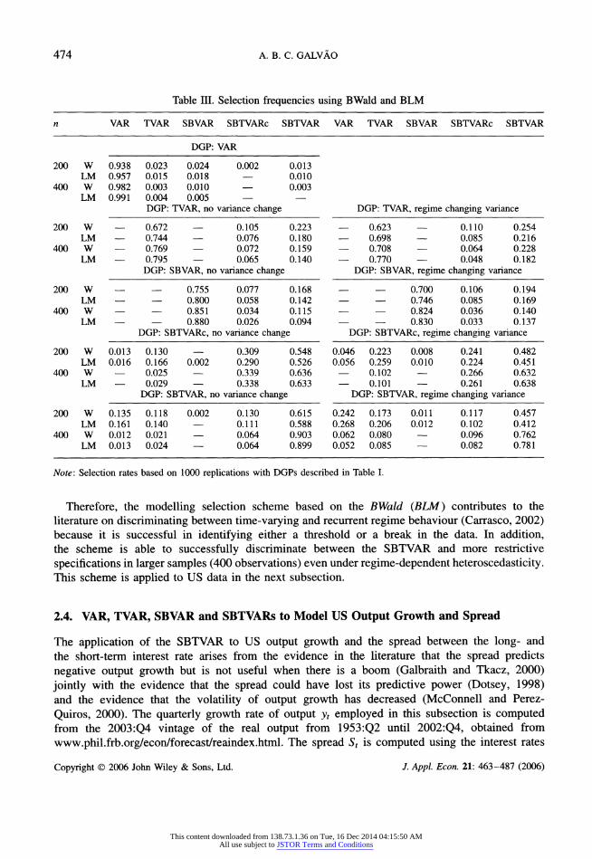
The selection frequencies presented in Table III show that the modelling strategy is successful in discriminating between VARs, TVARs and SBVARs. Because changes in the thresholds across

subsamples do not imply extra autoregressive parameters in the estimation, the selection rule is

generally not able to discriminate between SBTVARc and SBTVAR. As the sample increases, the selection rule discriminates between TVARs and SBTVARs when the SBTVAR is the DGP. When

the TVAR is the DGP, the selection rule chooses the SBTVAR relatively frequently. There are no

large differences in the selection frequencies on employing either the LM or the Wald statistics

(similar to the results of Altissimo and Corradi, 2002). Heteroscedasticity reduces the power of the selection rule on discriminating between TVAR and SBTVAR, but it does not affect significantly the selection frequencies of other models.

These selection frequencies are not worse than in previous papers that have proposed methods to

discriminate between linear and non-linear specifications (Gonzalo and Pitarakis, 2002; Strikholm and Terasvirta, 2003). Figure 1 helps us to understand why it is hard to discriminate between these nested versions of TVAR and SBTVAR in small samples: their main difference is in the smoothness of the transition when changing from causality to non-causality. Yet the distinction between these models increases with the sample size.




474 A. B. C. GALVAO

Table III. Selection frequencies using BWald and BLM

n VAR TVAR SBVAR SBTVARc SBTVAR VAR TVAR SBVAR SBTVARc SBTVAR

DGP: VAR

200 W 0.938 0.023 0.024 0.002 0.013 LM 0.957 0.015 0.018 ? 0.010

400 W 0.982 0.003 0.010 ? 0.003 LM 0.991 0.004 0.005 ? ?

DGP: TVAR, no variance change DGP: TVAR, regime changing variance

200 W ? 0.672 ? 0.105 0.223 ? 0.623 ? 0.110 0.254

LM ? 0.744 ? 0.076 0.180 ? 0.698 ? 0.085 0.216

400 W ? 0.769 ? 0.072 0.159 ? 0.708 ? 0.064 0.228

LM ? 0.795 ? 0.065 0.140 ? 0.770 ? 0.048 0.182

DGP: SBVAR, no variance change DGP: SBVAR, regime changing variance

200 W ? ? 0.755 0.077 0.168 ? ? 0.700 0.106 0.194

LM ? ? 0.800 0.058 0.142 ? ? 0.746 0.085 0.169

400 W ? ? 0.851 0.034 0.115 ? ? 0.824 0.036 0.140

LM ? ? 0.880 0.026 0.094 ? ? 0.830 0.033 0.137

DGP: SBTVARc, no variance change DGP: SBTVARc, regime changing variance

200 W 0.013 0.130 ? 0.309 0.548 0.046 0.223 0.008 0.241 0.482 LM 0.016 0.166 0.002 0.290 0.526 0.056 0.259 0.010 0.224 0.451

400 W ? 0.025 ? 0.339 0.636 ? 0.102 ? 0.266 0.632 LM ? 0.029 ? 0.338 0.633 ? 0.101 ? 0.261 0.638

DGP: SBTVAR, no variance change DGP: SBTVAR, regime changing variance

200 W 0.135 0.118 0.002 0.130 0.615 0.242 0.173 0.011 0.117 0.457

LM 0.161 0.140 ? 0.111 0.588 0.268 0.206 0.012 0.102 0.412

400 W 0.012 0.021 ? 0.064 0.903 0.062 0.080 ? 0.096 0.762

LM 0.013 0.024 ? 0.064 0.899 0.052 0.085 ? 0.082 0.781

Note: Selection rates based on 1000 replications with DGPs described in Table I.

Therefore, the modelling selection scheme based on the BWald iBLM) contributes to the

literature on discriminating between time-varying and recurrent regime behaviour (Carrasco, 2002) because it is successful in identifying either a threshold or a break in the data. In addition, the scheme is able to successfully discriminate between the SBTVAR and more restrictive

specifications in larger samples (400 observations) even under regime-dependent heteroscedasticity. This scheme is applied to US data in the next subsection.

2.4. VAR, TVAR, SBVAR and SBTVARs to Model US Output Growth and Spread

The application of the SBTVAR to US output growth and the spread between the long- and

the short-term interest rate arises from the evidence in the literature that the spread predicts

negative output growth but is not useful when there is a boom (Galbraith and Tkacz, 2000)

jointly with the evidence that the spread could have lost its predictive power (Dotsey, 1998) and the evidence that the volatility of output growth has decreased (McConnell and Perez

Quiros, 2000). The quarterly growth rate of output yt employed in this subsection is computed from the 2003:Q4 vintage of the real output from 1953:Q2 until 2002:Q4, obtained from

www.phil.frb.org/econ/forecast/reaindex.html. The spread St is computed using the interest rates





Table IV. Estimated parameters (1953:Q2-2002:Q4)

VAR TVAR SBVAR SBTVARc SBTVAR

d ? 4 ? 4 4, 4

r _ 0.463 [0.20,0.62] ? 0.488 [0.47,1.23] 0.31 [0.16,0.54], 1.51 [1.29,1.79]

r ? ? 1985 :2 [1983 :2,1986:2] 1971:2 [1969:3,1972:4] 1981:1 [1980:1,1982:1] 1.007 0.924

b\ 0.718 0.972 0.929 0.653 0.811 0.536 0.230 0.573 0.353

0.466 0.157

0.130 0.408

o\ 0.274 0.496 0.326 0.023 0.079 0.139 0.118 0.663 0.211

0.178 0.172

22 27 T 195 47 124 46 80

148 71 26 39 101 49

SIC-1.265 -1.412 -1.324 -1.165 -1.211

Note: The numbers in [ ] are the 90% confidence interval computed by bootstrap. o\ and <r| are respectively the estimated

variance of output and spread equations for each regime with T observations.

of 10-year Treasury bonds and 3-month Treasury bills, obtained from www.stls.frb.org/fred. The

quarterly frequency is obtained by averaging the monthly spread over the quarter. The estimates (by HML) of all the possible alternative hypotheses of the modelling procedure of

the last subsection are presented in Table IV. The 90% confidence intervals for the thresholds and the break-point are computed by applying bootstrapping.1 The estimates are obtained assuming at least 15% of the observations in each regime and at least 30% of the observations in each

subsample, and at least 20% of the observations of each subsample in each regime in the case of SBTVARs. All models are estimated for the same autoregressive order, p = 3, that has been chosen with the Schwarz information criterion applied to the VAR. The delay is estimated using an additional loop in the grid search assuming that di ? 1 and du ? 4.

The information criterion (SIC) suggests gains from the presence of a break-point and a

threshold, but the model with smaller SIC is the TVAR. The SBTVAR implies a reduction of 4% of the SIC compared with the SBTVARc with only the estimation of one more parameter.

The thresholds of the TVAR and the SBTVARc have similar values, and their value is not

statistically different from the r\ of the SBTVAR. The break-points are statistically different across the models, but the break-points of the SBVAR and the SBTVAR are not far from each other: 1981:1 and 1985 :2. The 1985 break implies that the estimated variance of the output growth equation after the break is 1/3 of the variance before the break. Similar sized variance reduction is also observed in the SBTVAR estimates but not in the SBTVARc. A break around 1985 is associated with the decrease in the volatility of output growth (McConnell and Perez-Quiros,

1 Data is simulated from the estimated model by bootstrapping from the residuals. The simulated data is employed to estimate thresholds and/or breaks (by HML together with the autoregressive parameters). The procedure is repeated 500 times and the limits of the 90% empirical interval are computed.




476 A. B. C. GALVAO

Table V. LM bounds (sample: 1953:Q2-2002:Q4)

Ho x HA BWald BLM

IA VAR x TVAR 1.602 1.497 IB VAR x SBVAR 1.134 1.095

2A1 TVAR x SBTVARc 1.476 1.393 2A2 TVAR x SBTVAR 1.695 1.572

2B1 SBVAR x SBTVARc 1.876 1.713 2B2 SBVAR x SBTVAR 2.064 1.852

XI TVARx3R-TVAR 0.807 0.792

X2 SBVAR x 2-SBVAR 1.261 1.190

Note: Selection rule: if BWald {BLM) > 1, then choose

model under alternative.

2000). In addition, Chauvet and Potter (2002) show that the presence of a break in 1985 improves forecasts using the spread as leading indicator and the probit as filter.

Table V presents the BWald and BLM for all possible tests of the two-step model selection

procedure. In the first step, the TVAR is chosen and in the second step the SBTVAR. This result

indicates that models with time-varying thresholds improve significantly over models with constant

thresholds and that the SBTVAR specification is chosen by the data. The table also presents BWald

and BLM to verify the need for an extra break in a SBVAR and an extra threshold in a TVAR.

There is evidence of a second break, but this model is not employed in the forecasting evaluation

because a careful analysis shows that this break is associated with the effect of the 1979-82

monetary policy in the dynamics of the spread and does not affect the predictive performance of

the spread.

Summarizing, the results suggest that there is changing non-linearity in the dynamics between

US output growth and spread. The SBTVAR captures a significant increase in the threshold value

after a break in 1981. This implies that the ability of the spread in predicting output growth has

changed, but it will be checked whether this means that the spread is not a reasonable leading indicator in a forecasting exercise in Section 3.

Sensibility to New Information: Recursive Estimation with Real-Time Data

The SBTVAR is able to capture interesting features of the dynamic relationship between the spread and the output growth. However, if the purpose of the modeller is to use it for forecasting, the

parameters must be robust to the arrival of new information. In this section, real-time output data

is employed to recursively estimate the SBTVAR.

The first sample used to estimate the parameters is from 1953:Q2 to 1985:Q4. This sample uses

all the information available until 1986:Q1. At each new point in time, the models are re-estimated,

using the newer data vintage. This new vintage may include large revisions of the current and

previous data. Two major data revisions are discussed in Croushore and Stark (2001): from GNP

to GDP in 1992 and changes in the chain-weighting in 1996. There is also a major revision in

1999:Q4 and 2000:Q1 because of changes in the national accounting tables. In the period of these

revisions, the data availability shortened and starts in 1959:Q1. Thus it is expected that there will

be larger changes in the parameters in those periods. For comparative purposes, a TVAR, a SBVAR and a SBTVARc are also estimated recursively.

Thresholds, break-point and delays estimated with information available including the data





Recursive Estimates with Real-Time data for the delay

1 JUL LJ|L11V VII?

0.5 I.111111111111111111111111111111111111111111111111111111111111111111

\+ dTVAR -+- dSBTVARc -+- d1 SBTVAR -?- d2SBTVAR|

Recursive Estimates with Real-Time data for break-point

1985 j

*-~ r~x_+

1965 m^/++H^H^+^

1963 I"'"'''"'''" ".?. .

I-tTVAR tSBTVARc ??? tSBTVAR I

3 5 Recursive Estimation with Real-Time Data for thresholds

j: [j

,

1.5-- ^l

If A/fnjr^l F****

0.5 m,' " 11111.11 / U..y^LlL.in

"'

0 I i i i i i ' i i i i i i i i i i i i i i i i i i i i i i i i i i i i i i i i i i i i i.i i i i i i i i i i i i i i i i i i i i i

F? rTVAR ?>-rSBTVARc .

M SBTVAR -?- r2SBTVARl

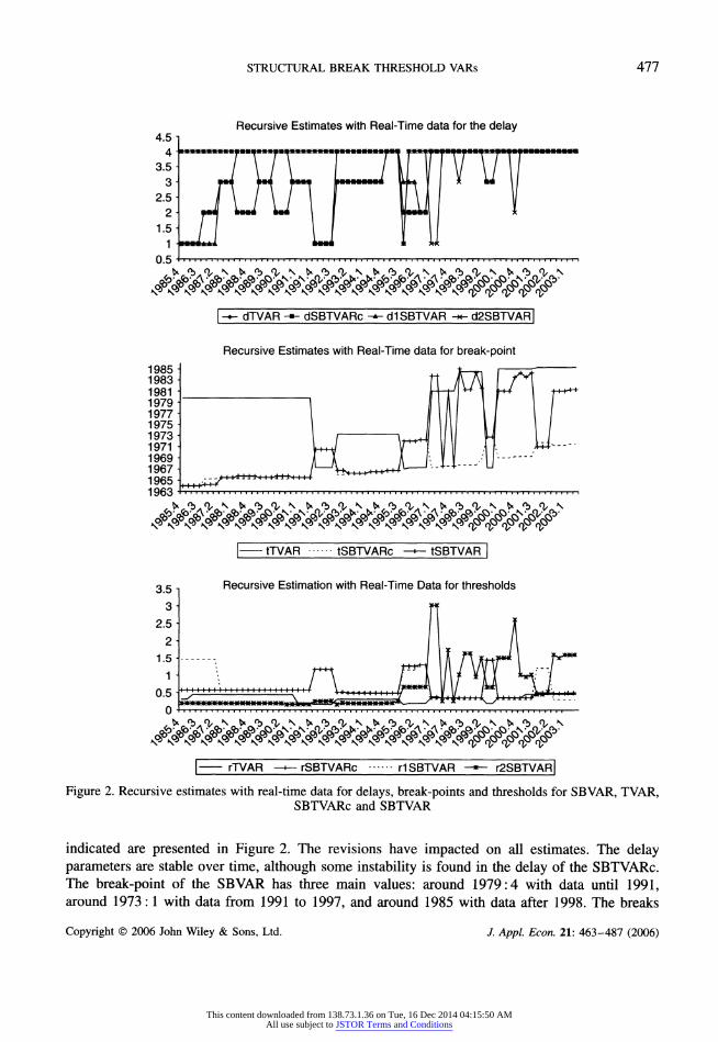
Figure 2. Recursive estimates with real-time data for delays, break-points and thresholds for SBVAR, TVAR, SBTVARc and SBTVAR

indicated are presented in Figure 2. The revisions have impacted on all estimates. The delay parameters are stable over time, although some instability is found in the delay of the SBTVARc. The break-point of the SBVAR has three main values: around 1979:4 with data until 1991, around 1973:1 with data from 1991 to 1997, and around 1985 with data after 1998. The breaks




478 A. B. C. GALVAO

could be associated with the productivity changes at the beginning of the 1970s, the monetary policy regime change in 1979 and the decreasing volatility at the beginning of the 1990s. This

stability is not found in the estimation of the break-point of the SBTVAR with data vintages after 1997. The estimates of break-points of these newer vintages oscillate between 1985 and 1972. This

oscillation of break-points between the early 1970s changes in productivity and the 1980s decrease in variability of output growth is also found by Chauvet and Potter (2002). Similar behaviour is found in the estimation of the thresholds: stability until 1996 for all the models and instability in the estimation of the second threshold of the SBTVAR model after that.

Summarizing, there is some instability in the definition of the break-point of the SBTVAR after 1997. This is not captured by the small 90% confidence interval presented earlier because,

when using all the information, the break-point is well identified. This sensibility may affect

out-of-sample forecasts in real time.

3. PREDICTING RECESSIONS

This section evaluates whether the proposed model, SBTVAR, is able to extract information from a leading indicator, the spread, in such a way that it improves forecasts of recessions.

3.1. Definition of Recession

Recessions are not directly observable in the data, but recessive periods can be identified based on simple rules applied to series that represent the aggregate economy. The rules employed in

this paper are based on those employed in the algorithms to identify turning points of classical business cycles. The advantage of employing simple rules to classify recessions is that the defined event can also be identified in forecast sequences, implying that probabilities of recession can

be computed.

In this paper, two definitions of recession are employed. The first definition of recession is: two

consecutive quarters of negative growth in the next five quarters (Fair, 1993). Thus, I state that the quarter t is in recession, so that Rt = 1, when there are two consecutive quarters of negative

growth in the window from t to t + 4. This definition of recession anticipates the NBER dates, so

that the ability of predicting this event means being able to anticipate NBER turning points. The second definition is based on a rule for identification of turning points: there is a recession

at t if either (y,_i < 0 and yt < 0) or (y, < 0 and yr+i < 0). The definition of this event is relevant

in real time because normally only y,_i is known and it is subjected to revision. This is a rare

event that occurs only in 10% of the quarters of the sample. An advantage of the definition of this event is that it identifies the same quarters in recession as the NBER with data after 1983, which

comprises the out-of-sample period employed in the forecasting evaluation.

The computation of the predictive probabilities of these events using estimated VARs employs simulation of forecast sequences in which the events are identified in such a way that the predictive

probability is the proportion of occurrences of the event after simulating a large number of

sequences (Anderson and Vahid, 2001). The complete procedure is described in the Appendix.

3.2. Measuring Loss from Event Forecasting

A forecaster has to decide whether to predict a recession or not based on a model that generates

probabilities of recessions Pt = Pr[recessionr|?2r_i] where ?lt-i is the set of information available





at t ? 1. The gain obtained by correctly predicting a recession is LQi) and the loss of wrongly

predicting a recession is L(fa). Thus, the loss function of the individual is L = Lifa) ?

LQi). The

individual will identify a recession when Pt > ct, therefore the decision of calling a recession will

be taken depending on the value of the cut-off ct and the predicted probabilities from the model.

Define Rt as the binary variable that defines whether the recession has occurred, then the gain of correctly calling a recession is LQi) =

fihict, Pt, Rt)). In particular, the gain from the correct

prediction as the percentage of successes/hits (so each hit gives exactly the same gain) is:

n

?>,l(P,>c) Lih) = Hie) = -^-=

nR

where 1() is an indicator function and R is the unconditional probability of the event recession.

The loss from false alarms is equal to the proportion of wrong predictions of recessions over the

number of recessive events, then the impact on a false alarm in the individual's loss is the same

as the hits: n

YJ(i-*,)i(P, >c)

Ufa) = FA(c) = ^-=

nR

Therefore, the loss function is:

1^2(1 -R,)KP, > c)\ -

(?*,l(P,>c)J Uc) =

Ai=!-4?^- (1) nR

This loss function has a resemblance to the Kuipers score (Pesaran and Skouras, 2002) but has a weight il/nR) for false alarms instead of 1/(1

? nR). Because the unconditional mean of the

recession is around 0.16 (for event A), the proposed loss function gives more weight to the losses

from false alarms than the Kuipers score. This loss function has the advantage of taking into

account the fact that the loss of wrongly predicting a recession is equivalent to the cost of not

predicting a recession, although the gains of correctly predicting a recession are higher than those of correctly predicting the expansion phase. Asymmetry in the loss function to evaluate recessions

has also been argued by Fintzen and Stekler (1999). The optimal choice of ct is the one that minimizes the loss function conditional on the past

values of Rt and Pt. In practice this can be done by calibrating the value of c using in-sample forecasts (for t =

1,... ,t ?

1), so that:

ct= min iLifaic))-Lihic))) (2)

The grid for the search is defined assuming that cL is equal to the unconditional probability of the event iR) and cv = 0.9. The events to be predicted have Ra = 0.16 and R^ = 0.10, so

the upper value of the grid allows a quite large interval to take into account characteristics of

the model employed to obtain Pt. The lower probability of the grid follows Birchenhall et al.

(1999), who argue in favour of a cut-off equal to the unconditional mean of the event because it allows us to check if the model adds information to a naive model that always predicts the unconditional mean. Based on ct estimated with in-sample predictions until t ?

1, the optimal




480 A. B. C GALVAO

decision for the individual is to call a recession when Pt >ct. This decision rule has an associated loss function L = L(fa(c))

? L(h(c)). Therefore, recession forecasters are ranked using this loss

function calculated for recursive forecasts for t = 1,..., n.

Even though the defined loss function is able to measure whether the model forecasts correctly the timing of the recession, the accuracy of the predictions could also be evaluated employing the

quadratic probability score (QPS). This measure of accuracy is based on a quadratic loss function which is also used to derive the mean of squared forecast errors of point forecasts. The QPS is

computed as follows:

1 n

QPS=-Y](Pt-Rt)2 (3)

The differential of this measure is that it does not depend on the definition of a cut-off and gives the same weight for large and small forecast errors and also for recessions and expansions.

3.3. Evaluating the Predictions of Probability of Recessions

The ability of the models to predict the probability of recession is evaluated under two scenarios. The first one uses all the information available at 2003 :Q4, which includes output growth data until

2003:Q3. In this case, in-sample forecasts of the probabilities of each event are evaluated. Using the parameters estimated for the full sample, information on output growth and spread until t ? 1 is used to predict the probability of the event at t. The second scenario uses real-time information.

The forecast for t employs the t data vintage, implying that information until r ? 1 is employed to estimate the model.

In both scenarios, it is necessary to define the cut-off ct such that a recession is predicted. In the

first scenario, a constant cut-off of 0.5 is employed for all the models, allowing better comparison of in-sample performance of the models. This value is also employed by Birchenhall et al. (1999), Chauvet and Piger (2003) and Duecker (2005). In real time, an automated procedure is employed to estimate the optimal cut-off in each point in time as described in Section 3.2. The procedure

employs events that occurred four quarters before t ? 1 (i.e., t ? 5), because otherwise they would

not be defined in real time, and the past information available in a rolling window of 15 years of

in-sample forecasts (60 quarters). The results of the evaluation are presented in Table VI. There are gains of accuracy and timing

from having joint thresholds and a break-point in predicting the in-sample recessions as defined by event A. The gains in accuracy of the SBTVAR compared with the VAR are of 30%. In addition,

while the VAR predicts correctly 10% of the recession periods, the SBTVAR does that in 45% of

them without creating false alarms. The gains of accuracy do not occur when predicting event B, but the SBTVAR is still the best for timing the recessions. The SBTVAR is able to predict two

out of the six recessive periods that happened after 1986, while the VAR is not able to predict recessions. Plots of the predicted probabilities of each model for each data vintage are presented in Figures 3 and 4.

The results using recursive estimation and real-time data show that the instability in the

estimation of the SBTVAR is translated to a weak forecast performance. Given the short sample sizes of the real-time exercise, it is reasonable to argue that it is necessary with all sample information to have good estimates of thresholds and breaks presented in the last section. In real

time, the TVAR is the best model to predict event A and the VAR is the best model to predict





Table VI. Measures of forecasting performance of the probability of recession

Sample VAR TVAR SBVAR SBTVARc SBTVAR

Event A

QPS In 1954:2-2003:3 0.093 0.074 0.097 0.072 0.066 1986:1-2003:3 0.086 0.080 0.112 0.070 0.063

RT 1986:1-2003:4 0.092 0.087 0.120 0.100 0.104

L(c) In 1954:2-2003:3 -0.097 -0.387 -0.226 -0.258 -0.452 1986:1-2003:3 0 -0.10 0 -0.20 -0.40

RT 1986:1-2003:4 0 -0.30 0.10 0 0

Event B

QPS In 1954:2-2003:3 0.059 0.046 0.058 0.057 0.048 1986:1-2003:3 0.045 0.044 0.048 0.036 0.037

RT 1986:1-2003:4 0.066 0.075 0.081 0.077 0.072

L(c) In 1954:2-2003:3 -0.059 -0.118 0.059 -0.059 -0.177 1986:1-2003:3 0 -0.167 0 -0.333 -0.333

RT 1986:1-2003:4 -0.167 0 0.167 0 0

Note: QPS is computed as in equation (3) and L(c) is defined in equation (1). In: in-sample; RT: real-time. Events A and B are defined in Section 3.1.

.9^ [ii? varin n no n n .9f- ni?tvarij n on n r

1960 1970 1980 1990 2000 1960 1970 1980 1990 2000

.9f- ||-SBVAR]| [] [If] [1 fl ,9 fMj-SBTVAR^j R Slfl fl \

1960 1970 1980 1990 2000 1960 1970 1980 1990 2000

Qp-fj-SBTVARl[j fl [Ifl fl f

.3- ~fo j' I M ik4^.vlUUJL,Jl.j/yL

1960 1970 1980 1990 2000

Figure 3. In-sample predictions of the probability of recession (event A, dotted line)

event B. This suggests that non-linearity is important in forecasting longer horizons because event A requires predictions of output growth up to five steps ahead. This result also suggests that the TVAR is a robust specification that can be employed successfully in real time.

Summarizing, gains from predicting recessions using SBTVARs are strong only when all samples are employed to estimate a break and thresholds. The TVAR and the VAR are robust specifications




482 A. B. C GALVAO

>9L |_

VARI | .gL I?TVARlt

| || | [

^ IMiLvUlJl. Jl,,. JL^L -1 [Aa. .MJL JH.Ji a_aJI . 1960 1970 1980 1990 2000 1960 1970 1980 1990 2000

.9f- |-SBVARI II II 9 D?ISBTVARcj R II (l I!

AM Jill .1 1.1 '*lL Mil 1 IL 11, 1960 1970 1980 1990 2000 1960 1970 1980 1990 2000

gp?|SBTVARl 0

I f]

1 y am^vAAji, ji.fi.j__ 1960 1970 1980 1990 2000

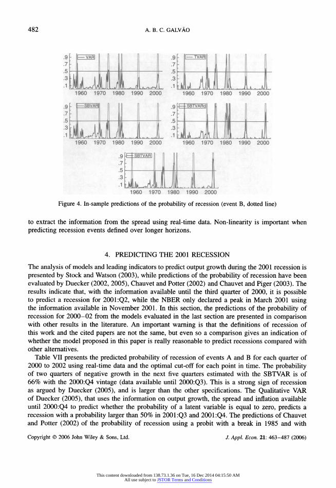
Figure 4. In-sample predictions of the probability of recession (event B, dotted line)

to extract the information from the spread using real-time data. Non-linearity is important when

predicting recession events defined over longer horizons.

4. PREDICTING THE 2001 RECESSION

The analysis of models and leading indicators to predict output growth during the 2001 recession is

presented by Stock and Watson (2003), while predictions of the probability of recession have been evaluated by Duecker (2002, 2005), Chauvet and Potter (2002) and Chauvet and Piger (2003). The results indicate that, with the information available until the third quarter of 2000, it is possible to predict a recession for 2001 :Q2, while the NBER only declared a peak in March 2001 using the information available in November 2001. In this section, the predictions of the probability of recession for 2000-02 from the models evaluated in the last section are presented in comparison

with other results in the literature. An important warning is that the definitions of recession of

this work and the cited papers are not the same, but even so a comparison gives an indication of whether the model proposed in this paper is really reasonable to predict recessions compared with other alternatives.

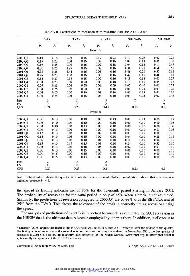
Table VII presents the predicted probability of recession of events A and B for each quarter of 2000 to 2002 using real-time data and the optimal cut-off for each point in time. The probability of two quarters of negative growth in the next five quarters estimated with the SBTVAR is of 66% with the 2000:Q4 vintage (data available until 2000:Q3). This is a strong sign of recession as argued by Duecker (2005), and is larger than the other specifications. The Qualitative VAR of Duecker (2005), that uses the information on output growth, the spread and inflation available until 2000:Q4 to predict whether the probability of a latent variable is equal to zero, predicts a

recession with a probability larger than 50% in 2001 :Q3 and 2001 :Q4. The predictions of Chauvet and Potter (2002) of the probability of recession using a probit with a break in 1985 and with





Table VII. Predictions of recession with real-time data for 2000-2002

VAR TVAR SBVAR SBTVARc SBTVAR

Pt ct Pt ct Pt ct Pt ct Pt ct

Event A

2000:Q1 0.10 0.18 0.03 0.16 0.12 0.23 0.13 0.29 0.02 0.29

2000:Q2 0.15 0.23 0.04 0.16 0.02 0.16 0.02 0.18 0.06 0.31

2000:Q3 0.19 0.25 0.06 0.16 0.02 0.18 0.04 0.16 0.11 0.47

2000:Q4 0.31 0.25 0.25 0.16 0.02 0.16 0.30 0.20 0.66 0.51

2001.Q1 0.35 0.25 0.44 0.16 0.05 0.16 0.46 0.20 0.37 0.18

2001.-Q2 0.26 0.23 0.37 0.16 0.03 0.16 0.42 0.16 0.46 0.18

2001:Q3 0.12 0.23 0.16 0.18 0.02 0.16 0.19 0.16 0.00 0.27

200LQ4 0.08 0.23 0.09 0.20 0.03 0.18 0.10 0.16 0.05 0.18

2002:Q1 0.05 0.25 0.02 0.20 0.06 0.29 0.02 0.40 0.01 0.27

2002:Q2 0.04 0.25 0.02 0.20 0.00 0.16 0.01 0.25 0.01 0.20

2002:Q3 0.04 0.25 0.02 0.16 0.01 0.16 0.02 0.29 0.01 0.20

2002:Q4 0.05 0.25 0.04 0.18 0.03 0.16 0.03 0.25 0.02 0.42

Hits 3 3 0 2 3 FA 0 0 0 1 0

QPS 0.24 0.26 0.40 0.25 0.21

Event B

2000:Q1 0.01 0.13 0.01 0.10 0.02 0.13 0.01 0.13 0.00 0.18

2000:Q2 0.02 0.10 0.01 0.10 0.00 0.10 0.00 0.10 0.00 0.33

2000:Q3 0.03 0.30 0.02 0.13 0.00 0.10 0.00 0.10 0.00 0.35

2000:Q4 0.09 0.13 0.02 0.10 0.00 0.10 0.01 0.10 0.03 0.33

2001:Q1 0.17 0.13 0.03 0.10 0.02 0.10 0.03 0.10 0.08 0.10

2001:Q2 0.13 0.13 0.04 0.10 0.02 0.10 0.04 0.10 0.25 0.15

2001:Q3 0.05 0.13 0.08 0.10 0.01 0.10 0.11 0.10 0.00 0.15

200LQ4 0.13 0.13 0.15 0.15 0.08 0.10 0.24 0.10 0.33 0.10

2002:Q1 0.03 0.13 0.01 0.18 0.05 0.10 0.02 0.10 0.01 0.10

2002:Q2 0.01 0.13 0.00 0.15 0.00 0.10 0.00 0.10 0.00 0.10

20O2:Q3 0.01 0.15 0.00 0.10 0.00 0.10 0.01 0.10 0.00 0.10

2002:Q4 0.01 0.15 0.01 0.13 0.00 0.10 0.01 0.10 0.00 0.28

Hits 2 0 0 11 FA 1 0 0 1 1

QPS 0.20 0.23 0.24 0.23 0.21

Note: Bolded dates indicate the quarter in which the events occurred. Bolded probabilities indicate that a recession is

signalled because Pt > ct.

the spread as leading indicator are of 90% for the 12-month period starting in January 2001. The probability of recessions for the same period is only of 45% when a break is not estimated.

Similarly, the predictions of recession computed in 2000:Q4 are of 66% with the SBTVAR and of 25% from the TVAR. This shows the relevance of the break in correctly timing recessions using the spread.

The analysis of predictions of event B is important because this event dates the 2001 recession as

the NBER2 that is the ultimate date reference employed by other authors. In addition, it allows us to

2 Duecker (2005) argues that because the NBER peak was dated in March 2001, which is after the middle of the quarter,

the first quarter of recession is the second one and because the trough was dated in November 2001, the last quarter of recession is 2001 :Q4. I follow the quarterly dates presented on the NBER website (www.nber.org) to affirm that event B

gets exactly the quarters of the NBER recessions.




484 A. B. C. GALVAO

evaluate the ability of predicting recessions in short horizons. The SBTVAR predicts a recession in 2001 :Q2 (probability of recession is larger than the cut-off), implying that with information until 2001 :Q1, it is possible to identify a recession in 2001 :Q2 and 2001 :Q3. An earlier warning of recession (2001 :Q1) is given using the VAR. This confirms the results of Stock and Watson

(2003) that the spread is a good leading indicator of the 2001 recession, although this was not true when predicting the 1990-91 recession. The probit model with coefficients changing by

Markov-switching proposed by Duecker (2002) also gives a recession sign for 2001 :Q2 using the 3-month difference of the composite leading indicator. In contrast, the results of the Markov

switching model applied to real-time output growth presented by Chauvet and Piger (2003) indicate a probability of recession higher than 50% only in 2001 :Q3. This shows the relevance of the information of a leading indicator for real-time prediction.

Based on these results, one can conclude that the SBTVAR performs well in predicting the 2001 recession. Two factors are responsible for that: (a) time-varying non-linearity, a break and different thresholds in each subsample, is needed to predict recessions over longer horizons using the spread as leading indicator; and (b) the spread is a good leading indicator for the 2001 recession.

5. CONCLUSIONS

This paper proposes a VAR with time-varying threshold non-linearity, called a structural break threshold VAR (SBTVAR). When applied to US output growth and the spread (long- minus short term interest rate), the SBTVAR is able to characterize changes in the predictive ability of the

spread and in the volatility of the output growth. Real-time forecasts for the timing of the 2001

recession are improved by allowing time-varying thresholds.

A maximum likelihood (HML) estimator for the SBTVAR is shown to jointly estimate thresholds

and a break-point without bias in finite samples. A model selection procedure based on asymptotic bounds of supLM and supWald statistics (Altissimo and Corradi, 2002) is proposed to decide

whether there is a break and/or a threshold in a VAR. An evaluation of this selection procedure in finite samples shows that it is generally able to choose the correct model between a VAR, a

threshold VAR, a structural break VAR and a SBTVAR. When this selection procedure is applied to a VAR of US output growth and the spread, it suggests time-varying threshold non-linearity.

The SBTVAR captures a significant increase in the threshold value and a decrease in the variance

of the output growth equation after a break in 1981. However, the estimates are sensible to the

arrival of new information from new vintage data.

The SBTVAR is compared with a VAR and VARs with either breaks or thresholds in their

ability to predict recessions. Two recession events are defined based on forecast sequences output

growth: event A generally anticipates NBER turning points and event B mimics the turning points after 1983. The timing of predictions is evaluated using a loss function that gives equal weights to hits and false alarms, and the accuracy is assessed using the quadratic probability score. The

results indicate that: (a) gains from predicting recessions using SBTVARs are stronger only when

all information is employed to estimate a break and thresholds; (b) TVARs and VARs are robust

specifications to extract the information from the spread using real-time data; and (c) non-linearity is important when predicting recession events defined over longer horizons. A comparison of the

predictions for the 2001 recession from the SBTVAR with other models presented in the literature





shows that the SBTVAR performs well. Two factors are responsible for that: time-varying non

linearity is needed to predict recessions over longer horizons using the spread and the spread is a

good leading indicator for the 2001 recession.

The proposed SBTVAR could be employed in future research to extract information from other leading indicators or from the CLI. Based on the evidence of structural breaks in many

macroeconomic time series (Sensier and Van Dijk, 2001) and of non-linearity in some series

(Stock and Watson, 1999), the SBTVAR could also be employed to model dynamic relations between macroeconomic variables, such as unemployment, inflation and output growth.

APPENDIX

ALGORITHM TO OBTAIN PREDICTIVE PROBABILITIES FROM THE MODELS

The procedure to extract the probabilities of event A and B from the models is the same as the one

described by Anderson and Vahid (2001). Define Xf~l = [xt-\,xt-2,..., x\} as the history of xt and xt =

f(Xt~l\T) + ut as the forecasting model where T is the matrix of parameters, including thresholds and breaks when they are defined in the specification, and ut are i.i.d. with Var(?,) = ___.

Given ft and ___, the trial sequence of forecasts for {xt, xt+i,xt+2,xt+3, xt+$\ conditional on Xf~l is built as follows. A random vector ut is drawn by bootstrap from the residuals ut and used to calculate xt, given X*~l and p. xt is added to the 'history' to form Xf. Then a new draw (et+\) is made from the residuals and employed to calculate xt+\, given X* and /? and to form Xt+l.

This procedure is continued until the sequence of forecasts is complete {xt, ?,+_, x,+2. *h-3, ?.+4}. This sequence of forecasts can be called S\, and the same trial is repeated to obtain a set of 2000 forecast sequences. The probability of event A (B) is the proportion of these 2000 sequences in

which the event A (B) occurs (Pt). In the case of event B, information of xt-\ is added to the

sequence of forecasts to define whether the event is identified in each sequence. In the case of threshold VARs, the model can also be written as x{

= fJ(X*~l; T-7) + u\, where

j = 1, 2 for models with two regimes and j = 1, 2, 3, 4 for structural threshold models. Therefore,

Var(w/) depends on the regime (defined by the threshold and the transition variable), so for each

regime with different number of observations Tj f T = _C;=i Tj), there is a different _CJ and uj

is supposed to be multivariate normal with variance X.-7'. In this framework, for each step to obtain the forecast sequences (h

= 0, ..., 4) for, say, a two-regime threshold model, either vector

u)+h is drawn from u] or vector

uf+h is drawn from w2 depending on Sp+h-i-d < r ox Sj+h-i-d > r Then these vectors are employed to compute xt+h including the transition variable that defines the

regimes Sj+h-i-d- In the case of structural break VARs, the residuals are also drawn conditional on the subsample, allowing the variance to change depending on the period.

ACKNOWLEDGEMENTS

I would like to thank Mike Clements, Bill Russell, two anonymous referees, audiences at the RES Meeting at Warwick, the Common Features in Rio, the SBE Meeting in Salvador, and the members of the Statistics Department of the Stockholm School of Economics for many useful comments. Financial support from CNPq is gratefully acknowledged.

Copyright ? 2006 John Wiley & Sons, Ltd. J. Appl Econ. 21: 463-487 (2006)



486 A. B. C. GALVAO

REFERENCES

Altissimo F, Corradi V. 2002. Bounds for inference with nuisance parameters present only under the

alternative. Econometrics Journal 5: 494-519.

Anderson HM, Vahid F. 2001. Predicting the probability of a recession with nonlinear autoregressive leading indicator models. Macroeconomic Dynamics 59: 482-505.

Andrews DWK. 1993. Tests for parameter instability and structural change with unknown change point. Econometrica 61: 821-856.

Berk JM. 1998. The information content of the yield curve for monetary policy: a survey. De Economist

146: 303-320. Birchenhall CR, Jensen H, Osbom D, Simpson P. 1999. Predicting U.S. business-cycle regimes. Journal of

Business and Economic Statistics 17: 19-91.

Carrasco M. 2002. Misspecified structural change, threshold and Markov switching models. Journal of Econometrics 109: 239-273.

Chauvet M, Piger JM. 2003. Identifying business cycle turning points in real time. Federal Reserve Bank of St. Louis Review, pp. 47-61.

Chauvet M, Potter S. 2002. Predicting a recession: evidence from the yield curve in the presence of structural

breaks. Economics Letters 77: 245-253.

Clements MP, Galvao ABC. 2004. A comparison of tests of non-linear cointegration with an application to the predictability of the US term structure of interest rates. International Journal of Forecasting 20:

219-236.

Croushore D, Stark T. 2001. A real-time dataset for macroeconomists. Journal of Econometrics 105:

111-130.

Dotsey M. 1998. The predictive content of the interest rate term spread for future economic growth. Federal

Reserve of Richmond, Economic Quarterly 84: 31-51.

Duecker MJ. 1997. Strengthening the case for the yield curve as a predictor of US recessions. Federal

Reserve Bank of St. Louis Review, pp. 41-51.

Duecker MJ. 2002. Regime-dependent recession forecasts and the 2001 recession. Federal Reserve Bank of St. Louis Review, pp. 29-36.

Duecker MJ. 2005. Dynamic forecasts of qualitative variables: a Qual VAR model of U.S. recessions. Journal

of Business and Economic Statistics 23: 96-104.

Estrella A, Hardouvelis GA. 1991. The term structure as a predictor of real economic activity. Journal of Finance 46: 555-576.

Estrella A, Mishkin FS. 1998. Predicting US recessions: financial variables as leading indicators. Review of Economics and Statistics 80: 45-61.

Estrella A, Rodrigues AP, Schich S. 2003. How stable is the predictive power of the yield curve? Evidence

from Germany and the United States. Review of Economics and Statistics 85: 629-644.

Fair RC. 1993. Estimating event probabilities from macroeconometric models using stochastic simulation. In

Business Cycles, Indicators, and Forecasting, Stock JH, Watson MW (eds). NBER, University of Chicago Press: Chicago; 157-178.

Fintzen D, Stekler HO. 1999. Why did forecasters fail to predict the 1990 recession? International Journal

of Forecasting 15: 309-323.

Galbraith JW, Tkacz G. 2000. Testing for asymmetry in the link between the yield spread and output in the G-7 countries. Journal of International Money and Finance 19: 657-672.

Gonzalo J, Pitarakis J-I. 2002. Estimation and model selection based inference in single and multiple threshold models. Journal of Econometrics 110: 319-352.

Hamilton JD, Kim DH. 2002. A re-examination of the predictability of economic activity using the yield spread. Journal of Money, Credit and Banking 34: 340-360.

Hansen BE. 1996. Inference when a nuisance parameter is not identified under the null hypothesis. Econometrica 64: 413-430.

Hansen BE, Seo B. 2002. Testing for two-regime threshold cointegration in vector error correction models.

Journal of Econometrics 110: 293-318.

Haubrich JG, Dombrosky AM. 1996. Predicting real growth using the yield curve. Federal Reserve Bank of

Cleveland, Economic Review 32: 26-34.

Kim C-J, Nelson CR. 1999. Has the US economy become more stable? A Bayesian approach based on a

Markov-switching model of the business cycle. Review of Economics and Statistics 81: 608-616.





Koop G, Potter SM. 2000. Nonlinearity, structural breaks, or outliers in economic time series? In Nonlinear

Econometric Modeling in Time Series, Barnett WA, Hendry DF, Hylleberg S, Terasvirta T, Tjostheim D,

Wiirtz A (eds). Cambridge University Press: Cambridge; 61-78.

Koop G, Potter SM. 2001. Are apparent findings of nonlinearity due to structural instability in economic

time series? Econometrics Journal 4: 37-55.

Lahiri K, Wang JG. 1996. Interest rate spreads as predictors of business cycles. In Handbook of Statistics,

Vol. 14, Maddala GS, Rao CR (eds). Elsevier: Amsterdam; 297-315.

Lundbergh S, Terasvirta T, Van Dijk D. 2003. Time-varying smooth transition autoregressive models. Journal

of Business and Economics Statistics 21: 104-121.

McConnell MM, Perez-Quiros G. 2000. Output fluctuations in the United States: what has changed since

early 1980s? American Economic Review 90: 1464-1476.

Pesaran MH, Skouras S. 2002. Decision-based methods for forecast evaluation. In A Companion to Economic

Forecasting, Clements MP, Hendry DF (eds). Blackweil: Oxford; 241-267.

Pesaran MH, Timmermann A. 2004. How costly is it to ignore breaks when forecasting the direction of a

time series? International Journal of Forecasting, forthcoming. Sensier M, Van Dijk D. 2001. Short-term volatility versus long-term growth: evidence in US macroeconomic

time series. Centre for Growth and Business Cycle Research, University of Manchester, Discussion Paper 8.

Stock JH, Watson MW. 1989. New indexes of coincident and leading economic indicators. NBER Macroe

conomics Annual 4: 351-394.

Stock JH, Watson MW. 1999. A comparison of linear and nonlinear univariate models for forecasting macroeconomic time series. In Cointegration, Causality and Forecasting: A Festschrift in Honour of Clive

Granger, Engle RF, White H (eds). Oxford University Press: Oxford; 1-44.

Stock JH, Watson MW. 2001. Forecasting output and inflation: the role of asset prices. NBER Working Paper 8180.

Stock JH, Watson MW. 2003. How did leading indicator forecasts do during the 2001 recession? Federal Reserve Bank of Richmond, Economic Quarterly 89: 71-90.

Strikholm B, Terasvirta T. 2003. Determining the number of regimes in a threshold autoregressive model

using smooth transitions. Department of Economic Statistics, Stockholm School of Economics (mimeo). The Economist. 2001. Don't mention the R-word: are economic forecasters wishful thinkers or wimps? The

Economist, printed edition, March 1.

Tsay RS. 1998. Testing and modeling multivariate threshold models. Journal of American Statistical

Association 93: 1188-1202.

Van Dijk D, Strikholm B, Terasvirta T. 2003. The effects of institutional and technological change and business cycle fluctuations on seasonal patterns in quarterly industrial production series. Econometrics

Journal 6: 79-98.

Watson MW. 1999. Explaining the increased variability in long-term interest rates. Federal Reserve Bank of Richmond, Economic Quarterly 85: 71-96.




structural break threshold vars for predicting us recessions using the spread

Documents