strike user manual
DESCRIPTION
strike out beybehTRANSCRIPT

Strike User Manual
Strike 3.0
User Manual
Schrödinger Press

Strike User Manual Copyright © 2015 Schrödinger, LLC. All rights reserved.
While care has been taken in the preparation of this publication, Schrödinger
assumes no responsibility for errors or omissions, or for damages resulting from
the use of the information contained herein.
Canvas, CombiGlide, ConfGen, Epik, Glide, Impact, Jaguar, Liaison, LigPrep,
Maestro, Phase, Prime, PrimeX, QikProp, QikFit, QikSim, QSite, SiteMap, Strike, and
WaterMap are trademarks of Schrödinger, LLC. Schrödinger, BioLuminate, and
MacroModel are registered trademarks of Schrödinger, LLC. MCPRO is a trademark
of William L. Jorgensen. DESMOND is a trademark of D. E. Shaw Research, LLC.
Desmond is used with the permission of D. E. Shaw Research. All rights reserved.
This publication may contain the trademarks of other companies.
Schrödinger software includes software and libraries provided by third parties. For
details of the copyrights, and terms and conditions associated with such included
third party software, use your browser to open third_party_legal.html, which is in
the docs folder of your Schrödinger software installation.
This publication may refer to other third party software not included in or with
Schrödinger software ("such other third party software"), and provide links to third
party Web sites ("linked sites"). References to such other third party software or
linked sites do not constitute an endorsement by Schrödinger, LLC or its affiliates.
Use of such other third party software and linked sites may be subject to third
party license agreements and fees. Schrödinger, LLC and its affiliates have no
responsibility or liability, directly or indirectly, for such other third party software
and linked sites, or for damage resulting from the use thereof. Any warranties that
we make regarding Schrödinger products and services do not apply to such other
third party software or linked sites, or to the interaction between, or
interoperability of, Schrödinger products and services and such other third party
software.
May 2015

Contents
Document Conventions .................................................................................................... vii
Chapter 1: Introduction to Strike .................................................................................. 1
1.1 Strike Overview.......................................................................................................... 1
1.2 Running Schrödinger Software .............................................................................. 1
1.3 Starting Jobs from the Maestro Interface ............................................................. 3
1.4 Citing Strike in Publications.................................................................................... 4
Chapter 2: Strike Tutorial................................................................................................... 5
2.1 Preparing for the Exercises ..................................................................................... 6
2.2 Setting Preferences................................................................................................... 7
2.3 Generating and Testing a QSPR Model for Aqueous Solubility ....................... 7
2.3.1 Importing Data .................................................................................................... 8
2.3.2 Preparing Test and Training Sets ........................................................................ 9
2.3.3 Building a Partial Least Squares Model ............................................................ 11
2.3.4 Examining PLS Model-Building Results............................................................ 13
2.3.5 Applying the Model to the Test Set ................................................................... 17
2.3.6 Calculating Univariate and Bivariate Statistics.................................................. 19
2.3.7 Model-Building Using Principal Component Analysis ....................................... 21
2.3.8 Model-Building Using Multiple Linear Regression ............................................ 23
2.4 Extracting Actives Using Atom-Pair Similarities ............................................... 24
2.4.1 Importing Active and Decoy Ligands ................................................................ 25
2.4.2 Seeding the Database and Designating Probes ............................................... 26
2.4.3 Running the Calculate Similarity Job ................................................................ 27
2.4.4 Applying Atom-Pair Similarity............................................................................ 27
2.5 Extracting Actives Using Descriptor Similarities from Molecular Properties..29
2.6 Estimating Activity by Creating a QSAR Model................................................. 31
2.6.1 Preparing the Data............................................................................................ 32
2.6.2 Model Generation ............................................................................................. 33
2.6.3 Applying the Model to the Test Set ................................................................... 35
Strike 3.0 User Manual iii

Contents
iv
Chapter 3: Running Strike from Maestro ............................................................. 39
3.1 Building a QSAR Model.......................................................................................... 40
3.1.1 Choosing Molecules and Descriptors ............................................................... 41
3.1.2 Choosing a Regression Method........................................................................ 41
3.1.3 Removing Outliers ............................................................................................ 42
3.1.4 Choosing an Activity Property........................................................................... 42
3.1.5 Examining and Using Results ........................................................................... 42
3.2 Predicting Properties Based on a QSAR Model ................................................ 43
3.3 Calculating Similarities .......................................................................................... 44
3.4 Principal Component Factor Analysis................................................................. 45
3.5 Calculating Univariate and Bivariate Statistics ................................................. 48
Chapter 4: Running Strike from the Command Line.................................... 49
4.1 Usage Summary ...................................................................................................... 49
4.2 Input File Examples ................................................................................................ 49
4.3 Input File Keywords ................................................................................................ 50
4.3.1 Mode Selection ................................................................................................. 50
4.3.2 File Specification Commands ........................................................................... 50
4.3.3 Alternative Naming Convention Commands ..................................................... 51
4.3.4 Commands for Reading/Writing CSV Files....................................................... 51
4.3.5 Commands for Build QSAR Model (train) Jobs................................................. 52
4.3.6 Commands for Descriptor Similarity (simil) Jobs .............................................. 53
4.3.7 Commands for Atom-Pair Similarity (apsimil) Jobs........................................... 53
4.3.8 Commands for Factor Reduction Jobs.............................................................. 54
4.3.9 Other Commands.............................................................................................. 54
4.3.10 Keyword Requirements for Various Job Types................................................ 55
Chapter 5: Statistical Definitions and Methods ................................................ 59
5.1 Univariate Statistics ................................................................................................ 59
5.1.1 Symbols ............................................................................................................ 59
5.1.2 Mean, Median, and Mode ................................................................................. 59
Schrödinger Software Release 2015-2

Contents
5.1.3 Variance and Deviation ..................................................................................... 60
5.1.4 Skewness and Kurtosis..................................................................................... 61
5.2 Bivariate Statistics: Covariance and Correlation .............................................. 62
5.3 Model-Building Methods ........................................................................................ 65
5.3.1 Independent and Dependent Variables............................................................. 65
5.3.2 Partial Least Squares........................................................................................ 66
5.3.3 Principal Component Analysis .......................................................................... 66
5.3.4 Multiple Linear Regression ............................................................................... 67
5.4 Model Analysis and Validation.............................................................................. 67
5.5 Outlier Detection...................................................................................................... 68
5.6 Similarity Statistics ................................................................................................. 69
5.6.1 Atom-Pair Similarity .......................................................................................... 69
5.6.2 Similarity Measures in Descriptor Space .......................................................... 70
5.7 References................................................................................................................ 71
Getting Help ............................................................................................................................. 73
Index .............................................................................................................................................. 77
Strike 3.0 User Manual v

vi
Schrödinger Software Release 2015-2
Document Conventions
In addition to the use of italics for names of documents, the font conventions that are used inthis document are summarized in the table below.
Links to other locations in the current document or to other PDF documents are colored likethis: Document Conventions.
In descriptions of command syntax, the following UNIX conventions are used: braces { }
enclose a choice of required items, square brackets [ ] enclose optional items, and the barsymbol | separates items in a list from which one item must be chosen. Lines of commandsyntax that wrap should be interpreted as a single command.
File name, path, and environment variable syntax is generally given with the UNIX conven-tions. To obtain the Windows conventions, replace the forward slash / with the backslash \ inpath or directory names, and replace the $ at the beginning of an environment variable with a %at each end. For example, $SCHRODINGER/maestro becomes %SCHRODINGER%\maestro.
Keyboard references are given in the Windows convention by default, with Mac equivalents inparentheses, for example CTRL+H (H). Where Mac equivalents are not given, COMMANDshould be read in place of CTRL. The convention CTRL-H is not used.
In this document, to type text means to type the required text in the specified location, and toenter text means to type the required text, then press the ENTER key.
References to literature sources are given in square brackets, like this: [10].
Font Example Use
Sans serif Project Table Names of GUI features, such as panels, menus, menu items, buttons, and labels
Monospace $SCHRODINGER/maestro File names, directory names, commands, envi-ronment variables, command input and output
Italic filename Text that the user must replace with a value
Sans serif uppercase
CTRL+H Keyboard keys
Strike 3.0 User Manual vii

viii
Schrödinger Software Release 2015-2
Strike User Manual
Chapter 1
Chapter 1: Introduction to Strike
1.1 Strike Overview
Strike is a chemically-aware statistical package which is integrated with Maestro to provide aflexible and intuitive interface. Employing molecular data generated by Schrödinger softwaresuch as QikProp, Glide, Liaison, or MacroModel, or from other sources such as experimentaldata or third-party software, Strike can be used to do the following:
• Generate basic univariate and bivariate statistics such as mean, median, mode, covari-ance, and correlations
• Generate structure-activity relationship hypotheses using rigorous statistical methods
• Run validation tools to assess the validity and predictive power of generated QSAR/QSPR models
• Employ such models as filters and predictive tools
• Perform similarity analysis in molecular property or 2-dimensional structural space.
This document provides a set of tutorial exercises using the capabilities of Strike, a descriptionof the Strike GUI in Maestro, a command line reference chapter, and definitions of some statis-tics terms and methods.
1.2 Running Schrödinger Software
Schrödinger applications can be run from a graphical interface or from the command line. Thesoftware writes input and output files to a directory (folder) which is termed the working direc-tory. If you run applications from the command line, the directory from which you run theapplication is the working directory for the job.
Linux:
To run any Schrödinger program on a Linux platform, or start a Schrödinger job on a remotehost from a Linux platform, you must first set the SCHRODINGER environment variable to theinstallation directory for your Schrödinger software. To set this variable, enter the followingcommand at a shell prompt:
csh/tcsh: setenv SCHRODINGER installation-directory
bash/ksh: export SCHRODINGER=installation-directory
Strike 3.0 User Manual 1

Chapter 1: Introduction to Strike
2
Once you have set the SCHRODINGER environment variable, you can run programs and utilitieswith the following commands:
$SCHRODINGER/program &$SCHRODINGER/utilities/utility &
You can start the Maestro interface with the following command:
$SCHRODINGER/maestro &
It is usually a good idea to change to the desired working directory before starting the Maestrointerface. This directory then becomes the working directory.
Windows:
The primary way of running Schrödinger applications on a Windows platform is from a graph-ical interface. To start the Maestro interface, double-click on the Maestro icon, on a Maestroproject, or on a structure file; or choose Start → All Programs → Schrodinger-2015-2 →Maestro. You do not need to make any settings before starting Maestro or running programs.The default working directory is the Schrodinger folder in your Documents folder.
If you want to run applications from the command line, you can do so in one of the shells thatare provided with the installation and have the Schrödinger environment set up:
• Schrödinger Command Prompt—DOS shell. • Schrödinger Power Shell—Windows Power Shell (if available).
You can open these shells from Start → All Programs → Schrodinger-2015-2. You do not needto include the path to a program or utility when you type the command to run it. If you wantaccess to Unix-style utilities (such as awk, grep, and sed), preface the commands with sh, ortype sh in either of these shells to start a Unix-style shell.
Mac:
The primary way of running Schrödinger software on a Mac is from a graphical interface. Tostart the Maestro interface, click its icon on the dock. If there is no Maestro icon on the dock,you can put one there by dragging it from the SchrodingerSuite2015-2 folder in your Applica-
tions folder. This folder contains icons for all the available interfaces. The default workingdirectory is the Schrodinger folder in your Documents folder ($HOME/Documents/Schrodinger).
Running software from the command line is similar to Linux—open a terminal window andrun the program. You can also start Maestro from the command line in the same way as onLinux. The default working directory is then the directory from which you start Maestro. You
Schrödinger Software Release 2015-2

Chapter 1: Introduction to Strike
do not need to set the SCHRODINGER environment variable, as this is set in your default envi-ronment on installation. To set other variables, on OS X 10.7 use the command
defaults write ~/.MacOSX/environment variable "value"
and on OS X 10.8, 10.9, and 10.10 use the command
launchctl setenv variable "value"
1.3 Starting Jobs from the Maestro Interface
To run a job from the Maestro interface, you open a panel from one of the menus (e.g. Tasks),make settings, and then submit the job to a host or a queueing system for execution. The panelsettings are described in the help topics and in the user manuals. When you have finishedmaking settings, you can use the Job toolbar to start the job.
You can start a job immediately by clicking Run. The job is run on the currently selected hostwith the current job settings and the job name in the Job name text box. If you want to changethe job name, you can edit it in the text box before starting the job. Details of the job settingsare reported in the status bar, which is below the Job toolbar.
If you want to change the job settings, such as the host on which to run the job and the numberof processors to use, click the Settings button. (You can also click the arrow next to the buttonand choose Job Settings from the menu that is displayed.)
You can then make the settings in the Job Settings dialog box, and choose to just save thesettings by clicking OK, or save the settings and start the job by clicking Run. These settingsapply only to jobs that are started from the current panel.
If you want to save the input files for the job but not run it, click the Settings button and chooseWrite. A dialog box opens in which you can provide the job name, which is used to name thefiles. The files are written to the current working directory.
The Settings button also allows you to change the panel settings. You can choose Read, to readsettings from an input file for the job and apply them to the panel, or you can choose ResetPanel to reset all the panel settings to their default values.
You can also set preferences for all jobs and how the interface interacts with the job at variousstages. This is done in the Preferences panel, which you can open at the Jobs section bychoosing Preferences from the Settings button menu.
Strike 3.0 User Manual 3

Chapter 1: Introduction to Strike
4
Note: The items present on the Settings menu can vary with the application. The descriptionsabove cover all of the items.
The icon on the Job Status button shows the status of jobs for the application that belong to thecurrent project. It starts spinning when the first job is successfully launched, and stops spinningwhen the last job finishes. It changes to an exclamation point if a job is not launched success-fully.
Clicking the button shows a small job status window that lists the job name and status for allactive jobs submitted for the application from the current project, and a summary message atthe bottom. The rows are colored according to the status: yellow for submitted, green forlaunched, running, or finished, red for incorporated, died, or killed. You can double-click on arow to open the Monitor panel and monitor the job, or click the Monitor button to open theMonitor panel and close the job status window. The job status is updated while the window isopen. If a job finishes while the window is open, the job remains displayed but with the newstatus. Click anywhere outside the window to close it.
Jobs are run under the Job Control facility, which manages the details of starting the job, trans-ferring files, checking on status, and so on. For more information about this facility and how itoperates, as well as details of the Job Settings dialog box, see the Job Control Guide.
1.4 Citing Strike in Publications
The use of this product should be acknowledged in publications as:
Strike, version 3.0, Schrödinger, LLC, New York, NY, 2015.
Schrödinger Software Release 2015-2

Strike User Manual
Chapter 2
Chapter 2: Strike Tutorial
This chapter is designed to help you become familiar with the functionality of Strike 3.0. Onceyou have worked through these exercises, you will have an understanding of the basic Strikefeatures.
The Strike workflow for QSAR model generation/validation generally consists of three steps:data preparation, model generation and validation, and model application. The Strike workflowfor similarity analysis using molecular properties also consists of three steps: data preparation,similarity calculation, and application of calculated similarities. For similarity analysis usingtwo-dimensional structures (atom-pair similarity), two steps are required: the similarity calcu-lation and application of calculated similarities. These steps will be illustrated in the tutorialexercises, which demonstrate how to do the following:
• Generate or import molecular data into Maestro for use by Strike• Generate, validate, and apply QSAR/QSPR models • Perform similarity analysis
Three tutorial examples are provided to demonstrate Strike workflows:
• Generating and testing a QSPR model for estimating aqueous solubility using a smallnumber of molecular properties
• Developing a QSAR model for predicting activities of folate-based thymidylate synthaseligands
• Calculating similarities using 2-dimensional structures and molecular properties, andwith these similarities extracting known actives for thermolysin from a ligand dataset.
To perform these exercises, you must have access to an installed version of Maestro. For instal-lation instructions, see the Installation Guide.
2.1 Preparing for the Exercises
To run the exercises, you need a working directory in which to store the input and output, andyou need to copy the input files from the installation into your working directory. This is doneautomatically in the Tutorials panel, as described below. To copy the input files manually, justunzip the strike zip file from the tutorials directory of your installation into yourworking directory.
Strike 3.0 User Manual 5

Chapter 2: Strike Tutorial
6
On Linux, you should first set the SCHRODINGER environment variable to the Schrödinger soft-ware installation directory, if it is not already set:
If Maestro is not running, start it as follows:
• Linux: Enter the following command:
$SCHRODINGER/maestro -profile Maestro &
• Windows: Double-click the Maestro icon on the desktop.
You can also use Start → All Programs → Schrodinger-2015-2 → Maestro.
• Mac: Click the Maestro icon on the dock.
If it is not on the dock, drag it there from the SchrodingerSuites2015-2 folder in yourApplications folder, or start Maestro from that folder.
Now that Maestro is running, you can start the setup.
1. Choose Help → Tutorials.
The Tutorials panel opens.
2. Ensure that the Show tutorials by option menu is set to Product, and the option menubelow is labeled Product and set to All.
3. Select Strike Tutorial in the table.
4. Enter the directory that you want to use for the tutorial in the Copy to text box, or clickBrowse and navigate to the directory.
If the directory does not exist, it will be created for you, on confirmation. The default isyour current working directory.
5. Click Copy.
The tutorial files are copied to the specified directory, and a progress dialog box is dis-played briefly.
If you used the default directory, the files are now in your current working directory, and youcan skip the next two steps. Otherwise, you should set the working directory to the place thatyour tutorial files were copied to.
csh/tcsh: setenv SCHRODINGER installation-path
sh/bash/ksh: export SCHRODINGER=installation-path
Schrödinger Software Release 2015-2

Chapter 2: Strike Tutorial
6. Choose Project → Change Directory.
7. Navigate to the directory you specified for the tutorial files, and click OK.
You can close the Tutorials panel now, and proceed with the exercises.
2.2 Setting Preferences
To keep the property list in the Project Table manageable, Maestro shows only the propertiesdesignated as “primary” for each application. In this tutorial, however, you will need access toall the properties, which you can do by setting a preference, as follows:
1. Click the Table button on the Project toolbar.
The Project Table panel opens.
2. Choose Table → Preferences.
The Preferences panel opens at the Project Table – Properties section.
3. Under When new entries are added, select Show all properties.
4. Close the Preferences panel.
2.3 Generating and Testing a QSPR Model for Aqueous Solubility
The aqueous solubility of organic molecules plays a key role in ADME processes, especiallyabsorption, distribution, and excretion. To experimentally measure accurate aqueous solubili-ties (logS) is difficult and requires a synthesis of the compound of interest. Because of this, anumber of in silico approaches have been developed to estimate this key molecular property,including fragment-based approaches, linear models, and non-linear models. QikProp,Schrödinger's molecular property predictor which estimates 44 molecular properties, uses alinear method for estimating logS.
The QikProp model, as with all linear or non-linear models, was fit to a finite set ofcompounds. When examining molecules outside the chemical space used in the fitting process,high accuracy in logS predictions might not be obtained. Consequently it may be desirable togenerate local QSPR (quantitative structure-property relationship) models relevant to thecompounds of interest. This tutorial provides an example of generating a local model for logSprediction using only molecular properties.
Strike 3.0 User Manual 7

Chapter 2: Strike Tutorial
8
2.3.1 Importing Data
1. Click the Import button on the Project toolbar.
2. In the Import dialog box, select the Maestro-format structure file aq_sol_ligs.maegz.
This file contains 1144 molecules for which experimental measurements of logS havebeen taken, as well as a set of calculated properties for each molecule.
3. If the import options are not displayed, click Options.
4. Ensure that Import all structures is selected.
5. Click Open.
The dialog box closes and the 1144 molecular structures in the file are imported. Theimport operation may take a minute to finish. When it has finished, the first structure inthe file is displayed in the Workspace.
6. If the Project Table panel is not open, click the Table button on the Project toolbar.
The Project Table panel opens.
As shown in Figure 2.1, each structure in the imported file is now an entry in the Project Table,represented by a row. The selected entries counter in the status bar of the panel reads 1144
selected. A long series of columns displays a number of molecular properties, or descriptors,which were calculated in advance for each entry. All but the first four columns (Row, Stars, In,and Title) can be scrolled into or out of view.
Schrödinger Software Release 2015-2

Chapter 2: Strike Tutorial
Figure 2.1. The Project Table after importing 1144 structures
Strike does not generate descriptors. The descriptors in this exercise came from three sources:
• Most of the descriptors in the table were determined by QikProp, a program distributedby Schrödinger that generates a widely applicable set of molecular properties. For moreinformation on QikProp, see the QikProp User Manual.
• A few descriptors were obtained from the ligparse utility ($SCHRODINGER/utilities/ligparse), including the Aromatic proportion and the Non-carbon propor-
tion. The aromatic proportion is the fraction of heavy atoms that are aromatic while thenon-carbon proportion is the fraction of heavy atoms that are not carbon.
• Also included are experimentally determined logS values in the measured log(solubil-
ity:mol/L) descriptor.
2.3.2 Preparing Test and Training Sets
The next step is to separate the 1144 molecules into two sets, a test set and a training set, usinga random selection method that is part of the Project Table facility.
1. In the Project Table panel, choose Select → Random.
The Random Selection dialog box opens.
2. Ensure that the value in the Randomly select n % of entries text box is 50, the default.
By default, the random set is chosen from only the selected entries. When the structurefile was imported, all entries were selected, but this may not always be the case.
Strike 3.0 User Manual 9

Chapter 2: Strike Tutorial
10
3. Change the Select from option from Selected entries to All entries and click Select.
After a moment, the Project Table is redisplayed with random entries selected. Theselected entries counter in the bottom of the panel now reads 572 selected.
To keep track of the newly selected entries, which will be used as the training set, add a columnto the Project Table that labels the currently selected molecules.
4. Choose Property → Add to open the Add Property panel.
5. In the Name text box, type Population.
6. Choose String from the Type option menu.
7. In the Initial value text box, type training. Click Add.
A column is added to the Project Table to the right of QPlogKhsa, as shown in Figure 2.2.Scroll to the far right to see this column. Under the column header Population, only thecurrently selected entries have a value of training.
Figure 2.2. The Project Table with a randomly selected training set
Because the random selection generator is machine-dependent, your training set is unlikely tobe a precise match to that shown in Figure 2.2, and therefore your results could differ fromthose shown in this document. Other results will also differ slightly because of differences inthe random selections made.
The data has now been prepared. In the next section, it will be used to generate a model.
Schrödinger Software Release 2015-2

Chapter 2: Strike Tutorial
2.3.3 Building a Partial Least Squares Model
It is known from the general solubility equation that a relationship exists between acompound’s aqueous solubility and its logP and melting points. We will use this idea in gener-ating our model by including the logP estimate from QikProp along with a handful of molec-ular properties chosen to fulfill the role of the melting point.
Your first model will use the Partial Least Squares (PLS) method, which is described briefly inChapter 5. Linear equations are generated that describe the relationship between a group offactors (derived from a set of independent descriptors) and a dependent descriptor (thepredicted property). The goal of PLS is to find factors that explain the variance in both theindependent and the dependent descriptors.
1. In the main Maestro window, choose Applications → Strike → Build QSAR Model orTasks → QSAR → Property-Based → Build Model.
The Build QSAR Model panel opens. As shown in Figure 2.3, the input counter under thepanel title bar reads Input is 572 entries currently selected in the Project Table.
Figure 2.3. The Build QSAR Model panel settings for the PLS model
Strike 3.0 User Manual 11

Chapter 2: Strike Tutorial
12
2. Under Available properties, control-click on the following properties:
• #rotor• Aromatic proportion• QPlogPo/w• volume
3. Under Add >, click Selected to move them to the Select descriptors to be included in the
model list.
The descriptor count is displayed: (4 currently selected) These four descriptors will be theindependent variables.
4. Ensure that the Regression method selected is Partial Least Squares.
5. Ensure that Automatically remove outliers is deselected (the default).
6. Enter 4 as the Maximum number of factors.
The Maximum number of factors should be less than or equal to the number of indepen-dent variables. If the Maximum number of factors is greater than the number ofindependent variables, Strike automatically reports the maximum number of factorsextracted from the data, which is generally equal to the number of independentdescriptors.
7. Select the Activity property (the dependent variable to be fit) by clicking Choose.
The Choose Activity Property dialog box opens.
8. Select measured log(solubility:mol/L) and click OK.
These settings mean that the model will attempt to correlate the number of rotatablebonds (#rotor), fractional aromatic proportion, molecular volume and logP (QPlogPo/w)to experimentally measured aqueous solubilities (measured log(solubility:mol/L)).
9. Enter solubility in the Job name text box.
10. Click Run to begin the calculation.
The job takes only a few moments to finish. When the model has been generated, theresults are incorporated into the Project Table, shown in Figure 2.4.
Schrödinger Software Release 2015-2
Chapter 2: Strike Tutorial
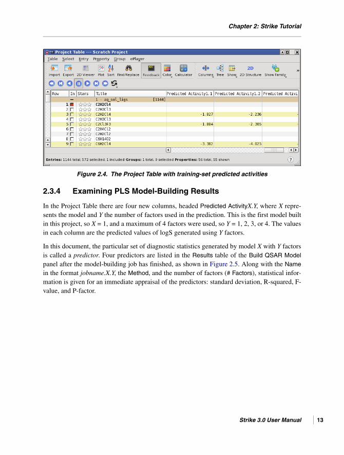
Figure 2.4. The Project Table with training-set predicted activities
2.3.4 Examining PLS Model-Building Results
In the Project Table there are four new columns, headed Predicted ActivityX.Y, where X repre-sents the model and Y the number of factors used in the prediction. This is the first model builtin this project, so X = 1, and a maximum of 4 factors were used, so Y = 1, 2, 3, or 4. The valuesin each column are the predicted values of logS generated using Y factors.
In this document, the particular set of diagnostic statistics generated by model X with Y factorsis called a predictor. Four predictors are listed in the Results table of the Build QSAR Model
panel after the model-building job has finished, as shown in Figure 2.5. Along with the Namein the format jobname.X.Y, the Method, and the number of factors (# Factors), statistical infor-mation is given for an immediate appraisal of the predictors: standard deviation, R-squared, F-value, and P-factor.
Strike 3.0 User Manual 13

Chapter 2: Strike Tutorial
14
Figure 2.5. The Build QSAR Model panel with a four-predictor PLS model
The five buttons below the Results table are now available. When a predictor is selected, thebuttons can be used to perform the following tasks. Some tasks affect only the selectedpredictor; others operate on the model as a whole, including any other predictors belonging tothe model:
Here, you will examine the 4-factor predictor by plotting its predictions for the training setversus measured log(solubility:mol/L).
1. Select the row named solubility.1.4 in the Results table and click Plot.
After a few moments, the Scatter Plot panel appears, showing measured logS values plot-ted against predicted values, with the line of best fit drawn.
Export Export the model for use in another project
View View the output file for the model-building job that generated the predictor
Plot Plot the predicted versus experimental results for the selected predictor
Delete Delete the model that generated the predictor
Predict Make further predictions using the selected predictor
Schrödinger Software Release 2015-2

Chapter 2: Strike Tutorial
By default, the plot facility automatically sets the range for the X and Y axes of the plot.However, it is easier to spot outlying points when the X and Y axes share a commonscale.
2. Select Equalize axis range.
The axis range changes so that both axes have the same range.
3. Select Equal aspect.
The plot is now drawn to a common scale, as in the example in Figure 2.6. Because thetraining set is selected randomly, some plot details will differ from yours.
Figure 2.6. Plot of predicted vs. measured logS for the training set
For most of the molecules in this training set, the generated model does a good job of repro-ducing experimental logS values, as can be seen in Figure 2.6. Next you will examine some ofthe cases where the model generates less accurate predictions:
1. In the Scatter Plot panel, click the Pick to include entries toolbar button.
2. Pick one of the data points for which the model is most in error.
The corresponding molecule is now included in the Workspace.
3. Pick other data points where the model is in error and look at their molecular structures inthe Workspace.
Strike 3.0 User Manual 15

Chapter 2: Strike Tutorial
16
The particular molecules you view will depend on the training set, but you should findthat the model does less well for molecules that contain long alkyl chains, sugar-like mol-ecules, and a few fused-ring heterocycles.
For information about other features of the Scatter Plot panel, click the Help button.
4. When you have finished working with the plot, close the panel.
More information about the model and the predictors is given in the output file of the model-building job, jobname.out, which can be examined using the View button:
1. In the Build QSAR Model panel, click the View button.
The View QSAR Model dialog box opens. This dialog box displays the output file for theStrike model-building job—see Figure 2.7.
Figure 2.7. The View QSAR Model dialog box
2. Examine the output file, noting the following points of interest:
• The Correlation Matrix for input variables (the four independent descriptors).
• PLS Regression Statistics, listing standard deviation (S.D.), R-squared, F-factor,and P-value by #Factors. The large F-factors and small P-values indicate this modelwas likely not achieved by chance and that the descriptors chosen are significant asa set.
• Cross Validation leave-N-out Results over M Cycles. Large differences between cal-culated q^2 and r^2 values reflect significant dependence of the model on the mole-cules included in the regression and in general are unfavorable.
• T-values and coefficients.
• Predicted values for logS at each #Factors for each of the molecules in the trainingset.
Schrödinger Software Release 2015-2

Chapter 2: Strike Tutorial
3. Click OK to close the View QSAR Model dialog box.
2.3.5 Applying the Model to the Test Set
The true test of any model is to check its predictions against a set of molecules not includedduring its training. The exercise performed in this section would typically be considered part ofmodel generation and validation, but for the purposes of this tutorial, it will be used to demon-strate the model application step of the Strike workflow.
The first step is to create a test set of molecules. In this example, the test set will be those mole-cules in the Project Table that were not members of the training set:
1. In the Project Table, confirm that the training set is selected by examining the Population
column. If so, skip to the next step.
If for any reason the training set is no longer the selected set—for example, if a singleentry has been selected instead—you can restore the selection by performing these steps:
a. Choose Select → Only from the Project Table.
The Entry Selection panel opens.
b. In the Properties list, select Population.
c. Select the option Is defined (any value).
Only the training set has a defined value (training) in the Population column.
d. Click Add, then OK.
The molecules in the training set, and only those molecules, are now selected.
2. In the Project Table, choose Select → Invert.
The selected molecules are now those that were not part of the training set. This will bethe test set.
Now you can run a prediction job on the test set molecules:
3. In the main window, choose Applications → Strike → Predict.
The Predict based on QSAR model panel opens. If it was open, the Build QSAR Model
panel closes.
In the Predict panel, the four predictors previously generated are listed in the Selectmodel to use for prediction table.
4. Select the model with 4 factors.
5. Click Run to launch the strike_predict job.
Strike 3.0 User Manual 17

Chapter 2: Strike Tutorial
18
The job takes a few seconds to run.
6. When the job is finished, view the Project Table.
There are four new columns to the right of the table: measured log(solubility:mol/L)
StrikePrediction(N), where N=1, 2, 3, or 4. These columns hold predicted logS values forthe test set, as shown in Figure 2.8.
Figure 2.8. The Project Table with test-set predicted solubilities.
Using the data in the fourth predicted values (N=4) column of the Project Table as thepredicted logS, plot the predicted logS versus measured log(solubility:mol/L) for the test setmolecules.
7. If the Manage Plots panel is not already open, open it by clicking the Plot button on theProject Table toolbar:
or choosing Table → Manage Plots.
8. Click New Scatter Plot.
A new Scatter Plot panel opens.
9. Choose measured log(solubility:mol/L) from the X-Axis option menu.
10. Choose measured log(solubility:mol/L) StrikePrediction(4) from the Y-Axis option menu.
The points are plotted in the plot area.
Schrödinger Software Release 2015-2

Chapter 2: Strike Tutorial
11. Select Equal aspect and Equalize axis range.
The plot should resemble that shown in Figure 2.9. The good agreement between calcu-lated and experimental values found for the training set remains quite good for the testset.
Figure 2.9. Plot of predicted vs. measured logS for the test set
12. Click the Pick to include entries toolbar button
13. Click on one or more of the less well-treated members of the test set.
As they appear in the Workspace, note that many are fused heterocycles, sugar-like mole-cules, or molecules with large aliphatic chains, as was observed in the training set.
14. When you have finished working with the plot, click Delete in the Manage Plots panel,then close the panel.
2.3.6 Calculating Univariate and Bivariate Statistics
The Strike statistics script calculates univariate and bivariate statistics of selected descriptorsfor the set of entries currently selected in the Project Table. The Strike Univariate and Bivariate
Statistics panel allows you to select from a list of the descriptors found in the Project Table.When you have run a statistics job, the results are displayed in the dialog box, from whichinformation can be copied and pasted to an open file as reference material or for printing.
Strike 3.0 User Manual 19

Chapter 2: Strike Tutorial
20
If for any reason the test set is no longer the selected set—for example, if a single entry hasbeen selected instead—you can restore the selection by performing these steps:
a. Choose Select → Only from the Project Table.
The Entry Selection panel opens.
b. In the Properties list, select Population.
c. Select the option Is defined (any value).
Only the training set has a defined value (training) in the Population column.
d. Click Add.
e. Click Invert and then OK.
The molecules in the test set, and only those molecules, are now selected.
1. Choose Applications → Strike → Statistics.
2. Select Aromatic_proportion from the list under Select one or two descriptors from the fol-
lowing list.
The selected descriptor is highlighted. This will be a univariate statistics calculation, sothe only input needed is the single descriptor you have selected.
3. Click Run to launch the job under the default name, strikeStats_1.
After a moment, the job results appear in the Results text area, as shown in Figure 2.10.These univariate statistics describe the range and variance of the descriptor values and theshape of the distribution for the test set of molecules (the currently selected entries in theProject Table). See Chapter 5 for definitions of statistics terms.
Now set up a bivariate statistics calculation.
4. In the descriptor list, select measured_log(solubility:mol/L), then control-click on #rotor.
5. Click Run.
After a few moments, the new results are appended to the Results table. They include asmall set of bivariate statistics for the pair of descriptors, followed by the univariate statis-tics for each, as shown in Figure 2.10. See Chapter 5 for definitions of statistics terms.
Schrödinger Software Release 2015-2

Chapter 2: Strike Tutorial
Figure 2.10. The Univariate and BIvariate Statistics panel with univariate statistics (left) and bivariate statistics (right)
2.3.7 Model-Building Using Principal Component Analysis
In this exercise, you will generate a model using one of the other alternative regressionmethods available in Strike, Principal Component Analysis.
1. In the Project Table, the test set is currently selected. Choose Select → Invert to select thetraining set.
2. Open the Build QSAR Model panel.
The Predict panel closes. The Build QSAR Model panel retains the selected descriptors,number of factors, and regression method used to generate the previous model. The fourpredictors generated by the PLS model-building job remain in the Results table.
3. Choose Principal Component Analysis from the Regression method option menu.
4. In the Job name text box, change the name to solubility_pca and click Run to launchthe calculation.
When the job has finished, the new model will be added to the Results table as a set ofpredictors with # Factors equal to 1, 2, 3, and 4, as was the PLS model. In the Eigenvaluecolumn, a number is associated with each of the four PCA-model predictors. The eigen-value represents the portion of the total variance accounted for by the n-factor predictor.
Strike 3.0 User Manual 21

Chapter 2: Strike Tutorial
22
In the Project Table, the four new columns Predicted Activity2.n are added to the table,with values only for the training set of molecules.
If you were using this PCA model in a real project, you could continue by carrying out theanalysis and prediction steps that were performed for the PLS model earlier in this chapter.
The PCA method is frequently used for data reduction by retaining only those factors neededto account for most of the total variance. The variance of each of the independent variablesused in the model is taken to be 1.0, and the total variance is defined as the sum of the vari-ances of each independent variable. Typically it is sufficient to retain only those factors with aneigenvalue greater than 1.0. These are the factors that account for more of the variance thandoes any single original variable.
In the Results table in the Build QSAR Model panel, the n-factor predictor of a PCA modelaccounts for a portion of the total variance equal to the sum of the first n eigenvalues. Forexample, in the table shown in Figure 2.11, the first eigenvalue is 1.92 and the second 1.29,while the third and fourth eigenvalues are less than 1.0. The total variance is 4.0, and the two-factor predictor is sufficient to account for (1.92 + 1.29)/4.00 = 80% of the total variance.
Figure 2.11. Build QSAR Model panel with four-predictor PCA model
Schrödinger Software Release 2015-2

Chapter 2: Strike Tutorial
2.3.8 Model-Building Using Multiple Linear Regression
The third regression method available for model-building in Strike is multiple linear regression(MLR). In this section, you will generate an MLR model that uses an algorithm to select theoptimal set of descriptors for use.
1. Ensure that the training set is selected in the Project Table.
2. In the Build QSAR Model panel, use control-click to select two more descriptors, mol MW
and SASA
3. Click Selected to add them to the Select descriptors to be included in the model list.
4. Choose Multiple Linear Regression from the Regression method option menu.
5. Select the Descriptors option Automatically select optimal subset.
6. Ensure that the Size of optimal subset is 4.
These settings instruct the MLR algorithm to use the best subset of four descriptors fromthe six selected.
7. Change the job name to solubility_mlr.
8. Click Run to launch the calculation.
The job takes only a few moments to finish. When the model has been generated, itappears in the Results table in the Build QSAR Model panel as a single row with MLRO
(MLR optimal subset) as the Method. See Figure 2.12.
The results are also incorporated into the Project Table as the column PredictedActivity3.1.
Strike 3.0 User Manual 23

Chapter 2: Strike Tutorial
24
Figure 2.12. Build QSAR Model panel with an MLR model
Again, you could continue with analysis and prediction using this model, as you did with thePLS model.
You can now close the Build QSAR Model panel.
2.4 Extracting Actives Using Atom-Pair Similarities
It is often useful to identify molecules that are “similar” in a chemically significant way tostructures of interest. Strike can be used to analyze similarity in either two-dimensional struc-tural (atom-pair connectivity) or molecular descriptor space. Using the atom-pair connectivitymethod has the advantage of requiring only structural (connectivity) information for a set ofprobe molecules and for the molecules for which calculated similarities are desired.
In this section, you will use Strike to calculate atom-pair similarities, then use those similaritiesto extract known actives for thermolysin from a ligand data set.
• If Maestro is already running, choose Close from the Project menu.
If the project is a scratch project from the previous exercises, you may discard it.
Schrödinger Software Release 2015-2

Chapter 2: Strike Tutorial
2.4.1 Importing Active and Decoy Ligands
First we need to create a ligand database which is seeded with a subset of the known activeligands. Using the remaining active ligands as probe molecules, we will attempt to extract theseeded actives out of the database.
1. Click the Import button on the Project toolbar.
2. In the Import dialog box, select the Maestro structure file 1tmn_actives.maegz.
This file contains nine known active ligands for thermolysin.
3. If the import options are not displayed, click Options.
4. Ensure that Import all structures is selected.
5. Click Open.
The first active ligand structure appears in the Workspace.
6. Open the Project Table panel.
There are nine entries, each with a Title identifying the ligand. Each row also has columnsof calculated molecular properties from QikProp. These properties will not be used in thisexercise, as they are not needed to generate atom-pair similarities.
7. Display each of the ligands in turn in the Workspace.
These structures show some diversity though many have peptide moieties.
Note: if the Workspace appears empty, click the Fit to Workspace toolbar button
to bring the ligand into view.
8. Click the Import button on the Project toolbar.
9. In the Import dialog box, select the file dl-400mw.maegz and click Open.
This file contains the Maestro-format structures of 998 decoy ligands with an averagemolecular weight of 400.
Strike 3.0 User Manual 25

Chapter 2: Strike Tutorial
26
After a few moments, the first decoy structure appears in the Workspace and 998 newentries are added to the Project Table. These entries also have molecular properties calcu-lated by QikProp, which will not be used in this exercise.
2.4.2 Seeding the Database and Designating Probes
At this point, all of the decoy ligands and none of the actives are selected in the Project Table.In this exercise, you will include three active ligands in the Workspace and add the other sixactive ligands to the selection to create the seeded ligand set.
1. Include the three active ligands, 1lna, 1tmn, and 5tln in the Workspace
Use control-click for the second and third ligands.
These three entries are not selected in the Project Table.
2. Add the six active ligands that are not included in the Workspace (1thl, 1tlp, 3tmn,4tmn, 5tmn, and 6tmn) to the selected entries by control-clicking their rows.
The database for which similarities will be calculated now contains 1004 entries, ofwhich six are known actives. The resulting Project Table is shown in Figure 2.13.
Figure 2.13. The Project Table with 1004 entries selected, 3 probes included.
Schrödinger Software Release 2015-2

Chapter 2: Strike Tutorial
2.4.3 Running the Calculate Similarity Job
1. Choose Applications → Strike → Similarity in the main window.
The Calculate similarity panel opens, as shown in Figure 2.14. As noted in the panel, sim-ilarity will be calculated for the entries selected in the Project Table, using the entriesincluded in the Workspace as probe molecules.
Figure 2.14. The Calculate Similarity panel with atom pair similarities specified.
2. Ensure that the Atom pair similarities option is selected.
3. Click Run.
Two columns are added to the Project Table upon completion of the job. For each entry, theMax AP Similarity is the maximum atom-pair similarity of that structure to any of the probemolecules, and the Mean AP Similarity is the mean of the atom-pair similarities to each of theprobes.
By default, atom-pair similarities are calculated on a scale from 0.0 to 1.0, with 0.0 indicatingno structural similarity and 1.0 indicating maximum structural similarity.
2.4.4 Applying Atom-Pair Similarity
In this exercise, you will examine how well atom-pair similarity performs in extracting the sixactive ligands (those not used as probes) from the set of decoy ligands. To do this, you will sortthe entries in the Project Table by similarity. Project Table entries (rows) can be sorted bymultiple user-specified properties (columns) called primary, secondary, and tertiary keys.
Strike 3.0 User Manual 27

Chapter 2: Strike Tutorial
28
When you imported the entries, they were grouped according to the file they were importedfrom. To sort the entries they must first be ungrouped.
1. In the Project Table, select the 1tmn_actives group, and the dl-400mw group.
2. Choose Entry → Group → Ungroup.
3. Right-click the Max AP Similarity column heading in the Project Table and choose Sort All
(Z to A).
The Project Table is sorted by descending Max AP Similarity, as in Figure 2.15.
Figure 2.15. The Project Table sorted by Max AP Similarity.
All six actives were found within the first 41 compounds (4.1% of the data set), and fivein the first 28 compounds (2.8% of the data set). The probe molecules are at the end of theProject Table.
4. As a second test, sort the Project Table again, repeating the previous step, but this timeusing Mean AP Similarity as the Primary Key.
Using the mean atom-pair similarities, all six actives are found in the first 21 compounds(2.1% of the data set).
It is not surprising that the mean atom-pair similarity does a better job of extracting activesfrom the data set than the maximum atom-pair similarity. Because all actives are at leastslightly structurally similar, their mean values are raised compared to decoy ligands, whichmay share common features with only one active molecule.
Schrödinger Software Release 2015-2

Chapter 2: Strike Tutorial
This example shows that Strike can be used to extract compounds similar to a set of moleculesusing 2D-geometry atom-pair similarities. Next, you will perform this extraction usingdescriptor similarity instead of atom-pair similarity.
2.5 Extracting Actives Using Descriptor Similarities from Molecular Properties
Now you will use calculated molecular properties to test the ability to extract actives from thedata set using descriptor similarities. The molecular properties for the thermolysin activeligands and decoy ligands were previously determined using QikProp. From this set of molec-ular properties, four descriptor-based similarities can be calculated: Euclidean similarity,Euclidean squared similarity, Manhattan similarity, and Tanimoto similarity. Each of thesemethods calculates the descriptor-space distance between two molecules as a function of theirmolecular properties. For a summary of each of these methods, see Chapter 5.
The calculated similarities for all but Tanimoto similarity are expressed as distances on an arbi-trary scale, where the smaller the value (the shorter the distance), the more similar the twomolecules. High values for these quantities correspond to longer distances in descriptor space,indicating less similarity.
The Tanimoto similarity is calculated on a scale from 0.0 to 1.0 with 1.0 indicating maximumsimilarity and 0.0 indicating no similarity.
Like atom-pair similarity, Strike calculates descriptor similarities for a set of molecules relativeto one or more probe molecules. The molecules included in the Workspace are used as probes;these molecules must also be included in the selected set (test set) of molecules.
1. In the Project Table, choose Select → All to select all entries.
2. Ensure that ligands 1lna, 1tmn, and 5tln are included in the Workspace.
If you are continuing from the previous exercise, they should be already included. Theseare the probe molecules, which must be both selected in the Project Table and included inthe Workspace.
3. If the Calculate similarity panel is not open, open it by choosing Applications → Strike →Similarity in the main window.
4. Select Descriptor similarities.
The Use descriptors list becomes available for choosing molecular properties to use incalculating similarities.
5. Select the donor HB and hb accptHB descriptors as shown in Figure 2.16 and click Run.
Strike 3.0 User Manual 29

Chapter 2: Strike Tutorial
30
Figure 2.16. The Calculate Similarity panel with descriptor similarities specified
After a few seconds the job finishes. In the Project Table, the calculated descriptor similaritieshave been added as properties. These properties include maximum and minimum distances aswell as the similarity measures.
In the descriptor similarity calculation, the molecular properties of the probe molecules areaveraged so they can be treated as a single virtual probe molecule. Similarity is calculated withrespect to only the selected properties. You will now examine how well descriptor similaritybased only on the number of hydrogen-bond acceptors and donors extracts known actives fromthe data set.
6. Right-click on the Euclidean sq property heading and choose Sort All (A to Z) to sort theproperty in ascending order.
The smallest values, corresponding to the greatest similarity to the probes, appear at thetop of the table. Of the 6 non-probe active ligands, 5 are found within the top 375 ligands.The remaining active, 1tlp, is ranked as last, due to its very large number of hydrogen-bond acceptor sites.
To find the actives:
a. Choose Table → Find/Replace or click the Find/Replace toolbar button.
b. Enter t in the Find text box.
Schrödinger Software Release 2015-2

Chapter 2: Strike Tutorial
c. From the Options menu, choose Selected properties only, and select the Title prop-erty in the dialog box.
d. Click Next.
7. Now sort based on Tanimoto in Descending order (sort twice).
Of the 6 non-probe actives, 5 are found in the top 560 compounds. The 1tlp ligand isagain the lowest-ranked active. You can find the actives by clicking Next on the Find tool-bar, as the search is already set up.
8. Close the Calculate Similarity panel, and hide the Find toolbar.
These very simple examples were designed to show possible applications of Strike similaritycalculations in descriptor and 2D-similarity space.
2.6 Estimating Activity by Creating a QSAR Model
In this tutorial, you will build a QSAR model and use it to predict activity. The most significantdifference between this exercise and the QSPR model-building exercise in Section 2.2 onpage 7 is that the property being predicted is a biological activity. The workflow and steps thatfollow are similar to the QSPR exercise.
Thymidylate synthase is an anticancer drug target as it catalyses the generation of deoxy-thymidine monophosphate given dUMP and a cofactor, 5,10-methylene tetrahydrofolate, anessential step in de novo DNA replication. The widely used anticancer agent 5-fluorouraciltargets thymidylate synthase and is active against solid tumors like breast, head, neck, andcolon cancers. Activities (EC50 and IC50) have been experimentally determined for a largeseries of compounds. You will use the set of broadly applicable descriptors generated byQikProp in order to develop a QSAR model with Strike.
For this tutorial, a set of 188 known inhibitors were selected. All of these ligands have experi-mentally-determined L1210 IC50 activities that range from 141 to 0.00052 μM. This set ofligands is well suited for QSAR as the structures have similar cores with a large variety ofsubstitution in shared side chains which leads to a wide activity range. The ligands wereprepared from 2D geometries using LigPrep, then neutralized, prior to being run throughQikProp to produce 36 predicted properties.
The Maestro format file thymidylate_synthase_ligands.maegz contains the 188 ligandstructures with their QikProp properties, their raw IC50 values, and their -log(IC50) values.Because the goal is a free energy relationship between activities and properties, you will usethe -log(IC50) or log(1/IC50) values rather than the raw IC50 values.
Strike 3.0 User Manual 31

Chapter 2: Strike Tutorial
32
• If Maestro is already running, choose Project → Close.
If the project is a scratch project from the previous exercises, you may discard it.
2.6.1 Preparing the Data
The ligand data must be imported into the project and divided into a test set and a training set.
1. Click the Import button.
2. In the Import panel, select the file thymidylate_synthase_ligands.maegz.
3. If the import options are not displayed, click Options.
4. Ensure that Import all structures is selected.
5. Click Open.
After a moment, the first ligand in the file appears in the Workspace.
6. Open the Project Table panel.
There are 188 entries in the project, all selected.
7. Choose Select → Random.
The Random Selection dialog box opens.
8. Ensure that the value in the text box is 50 and % of entries is chosen, then click Select.
After a moment, the Project Table is redisplayed with half the entries deselected at ran-dom. The selected entries counter in the status bar now reads 94 selected.
To keep track of the newly selected entries, which will be used as the training set, add a columnto the Project Table that labels the currently selected molecules:
1. Choose Property → Add to open the Add Property panel.
2. In the Name text box, type Population.
3. Choose String from the Type option menu.
4. In the Initial value text box, type training.
5. Click Add.
Under the column heading Population, only the currently selected entries have a value oftraining.
Schrödinger Software Release 2015-2

Chapter 2: Strike Tutorial
2.6.2 Model Generation
You will now build a QSAR model employing all of the relevant QikProp descriptors:
1. Choose Applications → Strike → Build QSAR Model in the main window.
The Build QSAR Model panel opens. The input counter under the title bar reads Input is 94entries currently selected in the Project Table.
2. If the Select descriptors to be included in the model list has any descriptors in it, click All
under < Remove.
3. Under Available properties, select all the descriptors (CTRL+A, A).
4. Control-click to deselect the following descriptors: Activity (-log[IC50]), #stars, #rtvFG,CNS, QPlogBB, and #metab.
The latter five descriptors are omitted because they are expected to be unrelated to thebinding process; the first will be the dependent variable.
5. Under Add >, click Selected.
The descriptors are transferred to the Select descriptors to be included in the model list.The Available properties list shows the properties you deselected.
6. Ensure that the Regression method is Partial Least Squares and that Automaticallyremove outliers is not selected.
7. In the Maximum number of factors box, type 20.
8. Click Choose.
The Choose Activity Property dialog box opens.
9. Select Activity (-log[IC50]) from the list and click OK.
See Figure 2.17 to check your settings.
Strike 3.0 User Manual 33

Chapter 2: Strike Tutorial
34
Figure 2.17. Build QSAR Model panel showing settings for activity model
10. In the Job name text box, enter strike_buildqsar.
11. Click Run to start the job.
When the job is finished, 20 potential models representing the 20 factors extracted are shownin the Results section of the Build QSAR Model panel. The predicted activities for all 20 factorsare added to the Project Table under the headers Predicted ActivityX.Y.
With 20 factors, the model fit to the 94 molecules in the training set should have a high Rsquared, a large F-statistic and a very small P-factor. The standard deviation (Std Dev) shoulddecrease from 1 to about 10 factors and then become somewhat constant while the R squared
value should increase continuously as more factors are included, leveling off at about 10factors. Thus, much of the predictive information is contained in the first 10 factors.
Inspect the results for the training set using the 10-factor predictor:
1. Select the 10-factor predictor (#Factors equal to 10) in the Results table.
2. Generate a plot of predicted activities versus experimental activities for the training set byclicking Plot. See Figure 2.18.
Schrödinger Software Release 2015-2

Chapter 2: Strike Tutorial
Figure 2.18. Plot of predicted vs. measured activity for the training set
3. When you have finished working with the plot, close the plot panel.
2.6.3 Applying the Model to the Test Set
The true test of any model is to check its predictions against a set of molecules not includedduring its training. The exercise performed in this section would typically be considered part ofmodel generation and validation, but for the purposes of this tutorial, it will be used to demon-strate the model application step of the Strike workflow.
The first step is to create a test set of molecules. In this example, the test set will be those mole-cules in the Project Table that were not members of the training set.
1. In the Project Table, confirm that the training set is selected by examining the Populationcolumn.
If so, skip to the next step. If for any reason the training set is no longer the selected set —for example, if a single entry has been selected instead — you can restore the selection byperforming these steps:
a. Choose Only from the Select menu of the Project Table.
The Entry Selection panel opens.
b. In the Properties list, select Population.
c. Select the option Is defined (any value).
Only the training set has a defined value (training) in the Population column.
Strike 3.0 User Manual 35

Chapter 2: Strike Tutorial
36
d. Click Add, then click OK.
The molecules in the training set, and only those molecules, are now selected. The mole-cules that were in the training set cannot be part of the test set, so you will invert theselection.
2. In the Project Table, choose Select → Invert.
3. In the Build QSAR Model panel, with the 10-factor predictor 1.10 selected, click Predict.
The Predict based on QSAR model panel opens showing all the models.
4. Ensure that the 10-factor predictor is selected as shown in Figure 2.19 and click Run.
Figure 2.19. Predict based on QSAR Model panel with 10-factor predictor selected
5. When the prediction job is finished, open the Project Table to view the new series of pre-dicted activities for the test set.
Now plot the results for the test set:
1. If the Manage Plots panel is not already open, open it by clicking the Plot button on theProject Table toolbar:
or selecting Plot from the Table menu.
2. Click New Scatter Plot.
A new Scatter Plot panel opens.
3. Choose Activity (-log[IC50]) from the X-Axis option menu.
Schrödinger Software Release 2015-2

Chapter 2: Strike Tutorial
4. Choose Activity (-log[IC50]) StrikePrediction(10) from the Y-Axis option menu.
The points are plotted in the plot area.
5. Select Equal aspect and Equalize axis range.
6. Select Diagonal line with slope.
A line with a slope of 1 (the default) is drawn on the plot. This is the line of perfect agree-ment. A sample plot is shown in Figure 2.20.
Figure 2.20. Plot of predicted vs. measured activity for the test set
The agreement between calculated and experimental values remains good for the test set. Indi-vidual data points of interest (outliers, high or low activity molecules) can be viewed in theWorkspace by clicking the In button, then choosing data points.
Strike 3.0 User Manual 37

38
Schrödinger Software Release 2015-2
Strike User Manual
Chapter 3
Chapter 3: Running Strike from Maestro
Before using Strike, molecular data (also referred to as “descriptor data”) should be obtainedand imported into the Maestro Project Table. This data can be generated using QikProp orother Schrödinger programs. Descriptors for ligands that bind to a receptor can be generatedusing the Ligand & Structure-Based Descriptors panel. This panel provides an interface toLiaison, Prime, MacroModel (eMBrAcE and ligparse), and QikProp to generate descriptors.For more information, see the document Ligand and Structure-Based Descriptors. Descriptorsgenerated by external programs or sources may be imported using standard comma-separatedvalue (CSV) format files.
Once the data is incorporated in the Project Table, you can perform statistical analyses andcreate and use QSAR models using the Strike panels in Maestro.
The Strike interface in Maestro consists of five panels:
• Build QSAR Model—Generate a QSAR model using a training set of molecules selectedfrom the Maestro Project Table, a set of independent descriptors, and a dependentdescriptor chosen from those available in the data.
• Predict based on QSAR model—Import a model or select one from the table of generatedmodels, then perform property predictions for molecules that were not part of the trainingset. Results can be viewed and unsatisfactory models can be deleted from the table.
• Similarity—Determine similarities in descriptor or 2D-structure space. Several distance-based descriptor similarity measures are available. Similarity in 2D-structure space isdetermined using an atom-pair-based approach.
• Factor Analysis—Perform a principal component analysis and display scores and load-ings plots for the principal components.
• Statistics—Display univariate and bivariate statistics.
These panels can be opened in Maestro from either Applications → Strike or Tasks → QSAR →Property-Based.
Strike 3.0 User Manual 39

Chapter 3: Running Strike from Maestro
40
3.1 Building a QSAR Model
You can use the Build QSAR Model panel to generate a QSAR model, given a training set ofmolecules selected from the Project Table, a set of independent descriptors, and a dependentvariable for which a prediction will be made.
To open the Build QSAR Model panel, choose Applications → Strike → Build QSAR Model orTasks → QSAR → Property-Based → Build Model. It may also be useful to open the ProjectTable containing your molecular data.
Figure 3.1. The Build QSAR Model panel
In this panel you can select the descriptors and activity property and choose a regressionmethod. When you have finished selecting options, you can name the job in the Job name textbox and click Run to run the job. For more information on starting jobs, including job settings,see Section 1.3 on page 3.
As the job starts, the job status icon on the Job toolbar rotates, indicating that a job is in prog-ress. If you want to view the job’s progress, click the job status icon (or choose Applications →Monitor Jobs). Most model-building jobs take only a few seconds to run.
Schrödinger Software Release 2015-2

Chapter 3: Running Strike from Maestro
Once a model has been built, 2D plots of predicted properties versus the dependent descriptordata can be created. Clicking points in a plot brings the molecule or molecules selected into theMaestro 3D Workspace for viewing and manipulation. (For more information about these andother Maestro plots, see Chapter 11 of the Maestro User Manual.)
From the Build QSAR Model panel you can proceed directly to the Predict based on QSAR
model panel or save the generated models in the project for later use.
3.1.1 Choosing Molecules and Descriptors
The first task in building a QSAR model is to select a training set of molecules in the ProjectTable. You can use the tools on the Select menu of the Project Table panel for this purpose.This menu includes a Random item that allows you to make a random selection of a percentageof either all molecules or the current selection of molecules. When you have made the selec-tion, the number of entries selected is displayed at the top of the Build QSAR Model panel.
The next step is to select a set of descriptors, which you do with the standard property selectiontools in the panel. Select the descriptors in the Available properties list, and click Selected tomove them to the Select descriptors to be included in the model list. You should choose anappropriate set of independent descriptors that is likely to correlate with the activity property.The number of descriptors chosen is displayed above the list. For the multiple linear regressionmethod, you have the option of choosing the optimal subset of these descriptors of a given size.
3.1.2 Choosing a Regression Method
Strike provides three regression methods: multiple linear regression (MLR), partial leastsquares regression (PLS), and principal component analysis (PCA). You can choose the regres-sion method from the Regression Method option menu. These methods have some commonoptions, and some unique options that are displayed or activated when you select the method.
Partial Least Squares (PLS)
When this method is selected, the Maximum number of factors text box is displayed. The rangefor Maximum number of factors is from 1 to the number of selected descriptors. The number ofmolecules selected to be used in building the model must be greater than or equal to themaximum number of factors. For more information about the method, see Section 5.3.2 onpage 66.
Principal Component Analysis (PCA)
When this method is selected, the Maximum number of factors text box is displayed. The rangefor Maximum number of factors is from 1 to the number of selected descriptors. The number ofmolecules selected must be greater than or equal to the number of descriptors chosen. For moreinformation about the method, see Section 5.3.3 on page 66.
Strike 3.0 User Manual 41

Chapter 3: Running Strike from Maestro
42
Multiple Linear Regression (MLR)
When this method is selected, the Descriptors options become available, and the Size of
optimal subset text box is displayed. The number of molecules selected must be greater than orequal to the number of initial descriptors. It is recommended that the number of molecules beat least five times greater than the number of descriptors.
If you want to use all descriptors, select the Descriptors option Use all selected descriptors1. Ifyou want Strike to determine the optimal subset of the selected descriptors, select Automatically
select optimal subset2, and enter a value in the Size of optimal subset text box. For more infor-mation about the method, see Section 5.3.4 on page 67.
If you want to force the regression line to pass through the origin, select y-intercept throughorigin.
3.1.3 Removing Outliers
Strike provides a means of automatically removing outliers, using the LOCI algorithm. Toremove outlying molecules before the model is built, select Automatically remove outliers. Bydefault, this option is not selected and outliers are not removed. For samples of 500 membersor more, selecting this option greatly increases the time needed for the model-building job. SeeSection 5.5 on page 68 for a description of the algorithm. Note that this option does not removeoutliers based on the model. If you wish to do so, you must run Strike from the command linewith the keyword printMLROutliers set.
3.1.4 Choosing an Activity Property
For the dependent variable, you must select a property that serves as the activity. This can beany property, experimental or computed. To select the property, click Choose. A propertyselector opens, in which you can select a single property from the Project Table. This is theproperty that you want the model to predict. When you choose the property, it is displayed inthe Activity Property text box.
3.1.5 Examining and Using Results
The Results table lists the models that have been calculated in the current Maestro project. Youcan select a single model to export, view, plot, delete, or use for prediction. Along with thename of each model, the table includes the regression method used, the number of PLS/PCAfactors or MLR descriptors, the eigenvalue for PCA models, and standard statistics values.
1. command-line keyword value MLRS2. command-line keyword value MLRO
Schrödinger Software Release 2015-2
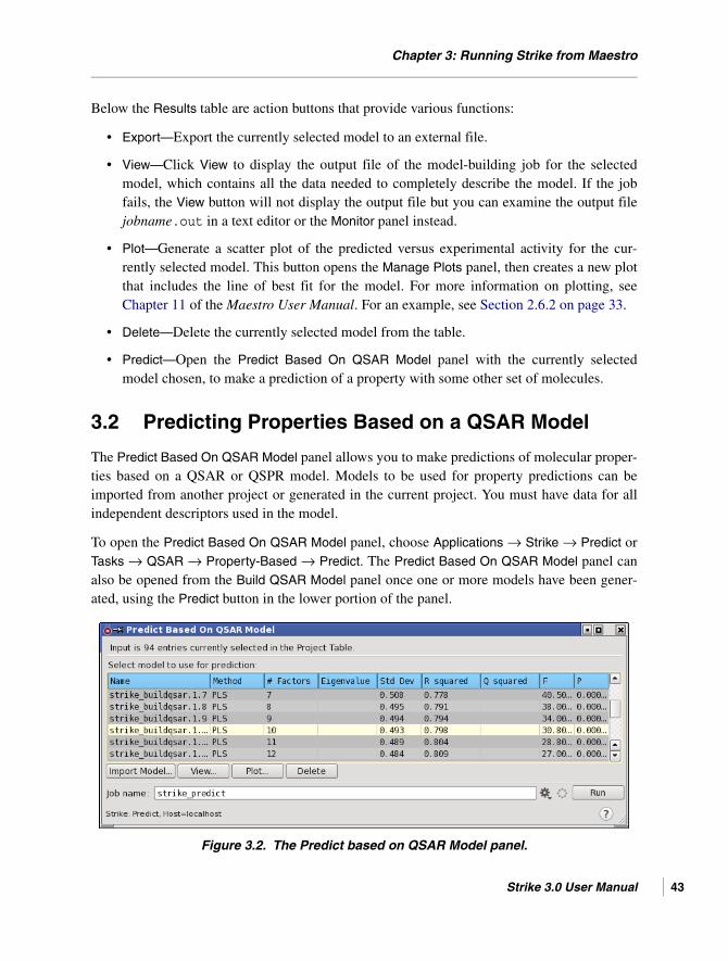
Chapter 3: Running Strike from Maestro
Below the Results table are action buttons that provide various functions:
• Export—Export the currently selected model to an external file.
• View—Click View to display the output file of the model-building job for the selectedmodel, which contains all the data needed to completely describe the model. If the jobfails, the View button will not display the output file but you can examine the output filejobname.out in a text editor or the Monitor panel instead.
• Plot—Generate a scatter plot of the predicted versus experimental activity for the cur-rently selected model. This button opens the Manage Plots panel, then creates a new plotthat includes the line of best fit for the model. For more information on plotting, seeChapter 11 of the Maestro User Manual. For an example, see Section 2.6.2 on page 33.
• Delete—Delete the currently selected model from the table.
• Predict—Open the Predict Based On QSAR Model panel with the currently selectedmodel chosen, to make a prediction of a property with some other set of molecules.
3.2 Predicting Properties Based on a QSAR Model
The Predict Based On QSAR Model panel allows you to make predictions of molecular proper-ties based on a QSAR or QSPR model. Models to be used for property predictions can beimported from another project or generated in the current project. You must have data for allindependent descriptors used in the model.
To open the Predict Based On QSAR Model panel, choose Applications → Strike → Predict orTasks → QSAR → Property-Based → Predict. The Predict Based On QSAR Model panel canalso be opened from the Build QSAR Model panel once one or more models have been gener-ated, using the Predict button in the lower portion of the panel.
Figure 3.2. The Predict based on QSAR Model panel.
Strike 3.0 User Manual 43

Chapter 3: Running Strike from Maestro
44
If you want to import a model into the table, click Import Model and navigate to the model(which has the extension .model). For example, you can import a model that was exportedfrom the Build QSAR Model panel in an earlier Strike session.
To make predictions:
1. Select the desired molecules in the Project Table.
The number of entries selected is displayed at the top of the panel.
2. Select the model to use for the prediction from the table.
This table contains information about each model in the current project. If you want toview complete information about the model, click View. The output file from the modelgeneration is displayed in a separate panel.
3. Name the job and click Run.
When the job finishes, the predictions are imported into the Project Table and are dis-played in the table.
To delete a model from the table, select it and click Delete.
To plot the results for a model, click Plot. This button opens the Manage Plots panel, thencreates a new, empty plot. You can then select the predicted and experimental properties to ploton the x and y axes, and display a linear regression line. For more information on plotting, seeChapter 11 of the Maestro User Manual. For an example, see Section 2.6.3 on page 35.
3.3 Calculating Similarities
The Calculate Similarity panel can be used to determine similarities in descriptor or 2D-struc-ture space. Several distance-based descriptor similarity measures are available. Similarity in2D-structure space is determined using an atom-pair-based approach.
Similarity, either atom-pair-based or descriptor-based, is calculated with respect to probe mole-cules. You select the probe molecules by including them in the Workspace. At least one mole-cule must be included in the Workspace, and at least one entry must be selected in the ProjectTable, before similarity calculations can proceed. For descriptor similarities, the probe mole-cules must also be selected in the Project Table.
To open the Calculate similarity panel, choose Applications → Strike → Similarity or Tasks →QSAR → Property-Based → Similarity.
Schrödinger Software Release 2015-2

Chapter 3: Running Strike from Maestro
Figure 3.3. The Calculate Similarity panel with descriptor similarities specified.
When you open the panel, the number of selected entries is displayed at the top of the panel.There are two options for the type of similarity to be calculated:
• Atom pair similarities—A similarity property will be created for each selected entry in theProject Table, based on the similarity of the atoms in the structure.
• Descriptor similarities—Similarity in terms of properties will be calculated for theselected Project Table entries in terms of the properties chosen from the Use Descriptors
list. When you choose this option, the Use Descriptors list becomes available. and youcan choose the properties you want to include in the similarity calculation. If you want toadjust the weights of the chosen descriptors in the evaluation of the similarity, clickAdjust Weight and set the desired weights in the Adjust Weight dialog box. The defaultweight is 1.0 for all descriptors.
3.4 Principal Component Factor Analysis
The Factor Analysis panel provides tools for performing principal component analyses ofvarious sets of descriptors taken from a set of entries that is selected in the Project Table. Oncean analysis is done, you can plot the scores and the loadings for selected pairs of principalcomponents, or make use of the principal component decomposition for further model genera-tion. For background on principal component analysis, see Section 5.3.3 on page 66.
The scores plot shows clustering of molecules from plotting one set of principal componentsagainst another. Each point on the plot represents a molecule. Molecules with similar data arefound together. Often it is possible to visually cluster molecules on the basis of the scores plot.
Strike 3.0 User Manual 45

Chapter 3: Running Strike from Maestro
46
The loadings plot (also known as a weights plot) shows the influence of individual variables(descriptors) on the principal components. Each point on the plot represents a variable from theinput data. Larger values for a given point indicates it has more weight in a given principalcomponent. Often it is possible to visually cluster the effect of variables on the principalcomponents.
By looking at a score and loading plot side-by-side it is possible to identify relationshipsbetween molecules and variables. For instance, if a number of molecules cluster with largevalues of the first principal component (PC1) in the scores plot, you can use the loadings plotto determine which variables have the most weight in PC1. These molecules will then clusternicely on the basis of those variables.
To generate the principal components:
1. Select the entries in the Project Table for which you want to perform the analysis.
2. Choose Factor Analysis from the Strike submenu of the Applications menu.
The Factor Analysis panel opens. The descriptor list is populated with the propertiesavailable in the Project Table. The visualization tools are hidden until an analysis job isrun.
Figure 3.4. The Factor Analysis panel before analysis
3. Select a set of descriptors from the descriptor list.
You can use shift-click and control-click in the usual way to select multiple list items.
Schrödinger Software Release 2015-2

Chapter 3: Running Strike from Maestro
4. Name the job in the Job name text box.
It is a good idea to choose a name that has some relation to the set of descriptors selected,since the name is displayed in the Visualize data from option menu once the first analysisjob finishes.
5. Click Generate Factors.
After a short time, the job finishes, and the visualization tools are displayed in the lowerpart of the panel.
Figure 3.5. The Factor Analysis panel after analysis
6. Repeat Step 3 through Step 5 for each set of descriptors that you want to analyze.
To display the results of an analysis:
1. Select the job from the Visualize data from option menu.
2. Select the principal components for the x and y axes for the desired plot types.
By default, component 1 and component 2 are selected.
3. Click the Plot Scores button.
The Manage Plots panel opens, and a new scatter plot with the selected data plotted isdisplayed. You do not need to close this panel to display another plot. For more informa-tion on these panels and plotting, see Chapter 11 of the Maestro User Manual.
4. Click the Plot Loadings button.
A panel opens with the loadings plotted and labeled.
Strike 3.0 User Manual 47

Chapter 3: Running Strike from Maestro
48
3.5 Calculating Univariate and Bivariate Statistics
The Univariate and Bivariate Statistics panel enables you to calculate univariate statistics orbivariate statistics over the entries that are selected in the Project Table. To display univariatestatistics for a particular descriptor, select the descriptor from the list of descriptors, then clickStart. To display univariate and bivariate statistics for a particular descriptor, select twodescriptors from the list of descriptors (click the first, control-click the second), then clickStart. The results are displayed in the Results text area. The statistics given are described inSection 5.1 on page 59 and Section 5.2 on page 62.
This panel obtains its descriptor information from the Project Table. If you subsequently add orremove properties (descriptors) from the Project Table, you need to close the panel and thenreopen it to capture the new information.
Figure 3.6. The Univariate and Bivariate Statistics panel with bivariate statistics
Schrödinger Software Release 2015-2

Strike User Manual
Chapter 4
Chapter 4: Running Strike from the Command Line
Strike can also be run using the strike command. This chapter lists keywords for the inputfile and gives two examples of command blocks that can be used in input files.
4.1 Usage Summary
$SCHRODINGER/strike [options] inputfile
4.2 Input File Examples
The strike input script consists of blocks of commands, each consisting of a series ofkeyword=value pairs and terminated by a line beginning with #. The termination line beginningwith # is mandatory, even if there is only one block of data in the input script. Each commandblock is then executed sequentially. Comment lines must begin with !!. Two examples ofcommand blocks are given below.
!! Section to train a modeldataFile=input_files/strike_mlro_fit.csvrunMode=trainmodel=MLROactivityLabel=activitynumOptDescript = 4# End of Section 1
!! Section to use a previously created model runMode=testdataFile=input_files/strike_pls_fit.csvmodelFile=input_files/strike_pls_fit.model# End of Section 2
inputfile The strike input script file containing the commands to be performed.
-HOST host Run job on a remote host.
-LOCAL Run the job in the current directory, rather than in a temporary scratch directory.
-WAIT Do not return until the job completes.
-NICE Run the job at reduced priority.
-HELP Print this message and exit.
Strike 3.0 User Manual 49

Chapter 4: Running Strike from the Command Line
50
4.3 Input File Keywords
The following keyword=value pairs are accepted input for strike. Boolean values must beexpressed as yes or no.
4.3.1 Mode Selection
All Strike jobs must use the runMode keyword with one of these values.
4.3.2 File Specification Commands
Value Description
train Generate a QSAR model.
test Predict properties using a QSAR model.
simil Run a descriptor similarity calculation.
apsimil Run an atom-pair (2D structure space) similarity calculation.
stats Generate statistics.
factorGen Extract factors from PCA model.
factorRed Reduce data using extracted PCA factors.
factorExp Expand reduced data using extracted PCA factors.
Keyword Value Description/Relevant Job Types
dataFile datafilename Keyword required for all jobs except atom-pair simi-larity (apsimil). File must be in CSV or Maestro format.
outputFile outputfilename Default is jobname.out. All jobs.
modelFile modelfilename Default is jobname.model. File containing QSAR model. QSAR jobs (train and test) and factor reduction jobs (factorGen, factorRed, factorExp).
csvFile csvoutfilename Default is jobname.csv. Output file containing all data used and generated in current command block. All jobs except apsimil.
plotFile qsaroutfilename File containing output from train with predicted vs. dependent data. QSAR jobs.
apPredFile filename File of molecules whose similarity to the probes are to be determined. apsimil jobs.
apActivesFile activesfilename File of probe molecules. apsimil jobs.
Schrödinger Software Release 2015-2

Chapter 4: Running Strike from the Command Line
4.3.3 Alternative Naming Convention Commands
4.3.4 Commands for Reading/Writing CSV Files
apInactivesFile inactivesfilename File of decoy molecules. apsimil jobs.
apWeightsFile weightsfilename Weights file. When generated, default is job-name.csv. apsimil jobs.
descriptorWeightFile weightsfilename Weights file. When generated, default is jobname-weights.tab. simil jobs.
Keyword Value Description/Relevant Job Types
modelTitle modelname Alternative title for QSAR model generation. Otherwise defaults to job-name.
baseName basename Alternative basename for all jobs. All output files will be basename.*, and modelTitle will default to basename.
Keyword Value Description/Relevant Job Types
delim string Delimiter character for reading .csv file. All jobs except apsimil.
includeColumns X:Y, Zcolumn numbers or column labels
X, Y, Z can be numbers or labels (headers). Use colon for ranges, For example, includeColumns=2:6,9,15 includes col-umns 2-6, 9, and 15 from the input file. All jobs except apsimil.
excludeColumns X:Y, Zcolumn numbers or column labels
X, Y, Z can be numbers or labels (e.g., labels:excludeColumns=IP(ev):QPlogKhsaProperties in .csv file between IP(ev) and QPlogKhsa, inclusive, will not be used). All jobs except apsimil.
includeRows X:Y, Zrow numbers or row labels
Include molecules (rows) specified. All jobs except apsimil.
excludeRows X:Y, Zrow numbers or row labels
Exclude molecules (rows) specified (e.g.,excludeRows=25 excludes molecule 25). All jobs except apsimil.
activityColumn integer Identify dependent property by column number. Build QSAR model jobs.
activityLabel label Identify dependent property by column label. Build QSAR model jobs.
Keyword Value Description/Relevant Job Types
Strike 3.0 User Manual 51

Chapter 4: Running Strike from the Command Line
52
4.3.5 Commands for Build QSAR Model (train) Jobs
rowHeaderColumn integer Set the column in the .csv file that contains row labels, by column numbering beginning at 1. For all jobs if needed.
rowHeaderLabel label Set the column in the .csv file that contains row labels by column label. For all jobs if needed.
descriptorWeightRow integer Set by number the row that contains the weight for each descriptor. For descriptor similarity jobs.
descriptorWeightLabel label Set by label the row that contains the weight for each descriptor. For descriptor similarity jobs.
Keyword Value Description/Relevant Job Types
model PLSPCAMLRSMLRONNET
Specify type of regression to be employed.
autoScale yes no
Set whether data is to be converted to a common scale. Default is yes.
maxFactors integer Maximum number of factors to return. PLS, PCA.
numOptDescript integer Number of descriptors to be retained, determined by optimization. MLRO.
removeOutliers no yes
Run prior to importing data into model building. Com-pare relative densities in descriptor space for included molecules to predict outliers. Recommended for sample size < 500 only. Default is no.
printMLROutliers no yes
Set to yes to output possible outliers with respect to the MLR model. Default is no. MLRS, MLRO.
MLROutlierCutoff integer Integer from 0 to 5 giving the number of MLR outlier tests that need to fail before a data point is identified as a possible model outlier. Default is 4. MLRS, MLRO.
lgoPercent double For leave-group-out (LGO) validation, percentage of fit-ting set to use as test set for each regression. Default is 5.0%
lgoCycles integer Number of cycles of LGO validation to perform. Default is 10.
RandCycles integer Number of randomization cycles to perform. Default is 10 times the number of independent descriptors. MLRS, MLRO, PLS, and PCA.
Keyword Value Description/Relevant Job Types
Schrödinger Software Release 2015-2

Chapter 4: Running Strike from the Command Line
4.3.6 Commands for Descriptor Similarity (simil) Jobs
4.3.7 Commands for Atom-Pair Similarity (apsimil) Jobs
supYintercept no yes
Suppress inclusion of the y intercept as a dependent vari-able for regression generation. The default is no, which means that the y intercept is included. MLRS, MLRO.
nnetNumUnitsInHiddenLayer
integer Number of units in the hidden layer. NNET.
nnetCrossValPer integer Percent of input data to be kept in the cross validation set. Default is 5%. NNET.
nnetExtValPer integer Percent of input data to be kept in the external validation set. Default is 10%. NNET.
nnetNumTrainCycles integer Number of training cycles for each neural network. Default is 200. NNET.
nnetNumNetworks integer Number of neural networks to train of which the best nnetumNetworksEnsem will be selected to create an ensemble neural network that is presented to the user. Default is 20. NNET.
nnetNumNetworksEnsem integer Number of the best neural networks to use in generating an ensemble neural network that is presented to the user. Default is 5. NNET.
Keyword Value Description
probes X:Y, Z Specify the probe molecules to use from the input file. X, Y, Z can be the molecule row indexes from the input file or, if rowHeaderColumn is defined, molecule titles.
simil euclidean Similarity
Keyword Value Description
apPredFormat maesdf
Format of apPredFile.
apActivesFormat maesdf
Format of apActivesFile.
apInactivesFormat maesdf
Format of apInactivesFile.
inactivePercent nn.n Percentage of inactives, e.g., for 99%: inactivePercent=99.0
Keyword Value Description/Relevant Job Types
Strike 3.0 User Manual 53

Chapter 4: Running Strike from the Command Line
54
4.3.8 Commands for Factor Reduction Jobs
4.3.9 Other Commands
readWeights yes no
Read weights from apWeightsFile.
genWeights yes no
Generate weights in apWeightsFile.
normalize range z-score none
Specify normalization approach. Default (range) normal-izes data to 0.0 - 1.0 scale; required for Tanimoto coefficient calculation. Specify z-score to scale data in standard deviation units. Specify none to perform no normalization.
Keyword Value Description
facRedAuto yes no
Determines if the factors are to be generated using scaled (yes) or unscaled (no) input data.
facRedNumFactors n Number of factors to generate. Range is from 0 to the num-ber of input data columns.
Keyword Value Description/Relevant Job Types
enrich Euclidean Euclidean_sq Tanimoto Manhattan
Calculate enrichment factors for extracting probe molecules from the entire data set, using the specified similarity mea-sure. For simil and apsimil jobs.
stats label Calculate univariate statistics for the descriptor label. Any job.
label1,label2 Calculate bivariate statistics for the descriptors label1 and label2. Any job.
Keyword Value Description
Schrödinger Software Release 2015-2
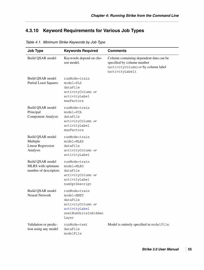
Chapter 4: Running Strike from the Command Line
4.3.10 Keyword Requirements for Various Job Types
Table 4.1. Minimum Strike Keywords by Job Type
Job Type Keywords Required Comments
Build QSAR model Keywords depend on cho-sen model.
Column containing dependent data can be specified by column number (activityColumn) or by column label(activityLabel).
Build QSAR modelPartial Least Squares
runMode=trainmodel=PLSdataFileactivityColumn or activityLabelmaxFactors
Build QSAR modelPrincipalComponent Analysis
runMode=trainmodel=PCAdataFileactivityColumn or activityLabelmaxFactors
Build QSAR modelMultiple Linear Regression Analysis
runMode=trainmodel=MLRSdataFileactivityColumn or activityLabel
Build QSAR modelMLRS with optimum number of descriptors
runMode=trainmodel=MLROdataFileactivityColumn or activityLabelnumOptDescript
Build QSAR modelNeural Network
runMode=trainmodel=NNETdataFileactivityColumn or activityLabelnnetNumUnitsInHiddenLayer
Validation or predic-tion using any model
runMode=testdataFilemodelFile
Model is entirely specified in modelFile.
Strike 3.0 User Manual 55

Chapter 4: Running Strike from the Command Line
56
Descriptor similarity calculation
runMode=simildataFileprobes(rowHeaderColumn or rowHeaderLabel)
One of the keywords in parentheses needed to specify probe molecules if probes not specified by molecule number.
Atom-pair similarity calculation.No weights
runMode=apsimilapActivesFileapActivesFormatapPredFileapPredFormat
Atom-pair similarity. Weights are generated and used in same command block
runMode=apsimilapActivesFileapActivesFormatapPredFileapPredFormatapInactivesFileapInactivesFormatinactivePercentgenWeights
Atom-pair similarity using weights that were generated previ-ously
runMode=apsimil apActivesFile apActivesFormat apPredFile apPredFormat readWeights apWeightsFile
PCA factor genera-tion
model=PCA runMode=factorGen facRedNumFactors facRedAuto=yes dataFile
Also generates reduced data set for the input.
Table 4.1. Minimum Strike Keywords by Job Type (Continued)
Job Type Keywords Required Comments
Schrödinger Software Release 2015-2

Chapter 4: Running Strike from the Command Line
PCA factor reduction model=PCA runMode=factorRed facRedNumFactors facRedAuto=yes dataFile modelFile
modelFile must be output of a factor genera-tion job. dataFile must contain the same descriptors as used in the factor generation, but need not contain data for the same structures.
PCA factor expansion model=PCA runMode=factorExp facRedNumFactors facRedAuto=yes dataFile modelFile
modelFile must be output of a factor genera-tion job. dataFile must be a file with reduced factors from a factor generation or reduction job.
Table 4.1. Minimum Strike Keywords by Job Type (Continued)
Job Type Keywords Required Comments
Strike 3.0 User Manual 57

58
Schrödinger Software Release 2015-2
Strike User Manual
Chapter 5
Chapter 5: Statistical Definitions and Methods
This chapter defines statistical quantities, algorithms, and regression methods used in Strike.
5.1 Univariate Statistics
This section defines some symbols, definitions, and equations relating to the statistics of asingle variable.
5.1.1 Symbols
N
Number of data points (observations) in a sample. There is no hard limit on sample size(number of molecules) in Strike, but for large samples (millions of molecules) practical issuessuch as system memory limitations may apply.
xi —value of data point i in a sample of variable x
x —mean of variable x
5.1.2 Mean, Median, and Mode
These statistics describe the “central tendency” of a variable.
Mean
The mean of variable x is defined by Equation (1).
(1)
Median
• For an even number of data points, the median is the mean of the middle-most two valuesin the ordered sample.
• For an odd number of data points, the median is the middle-most value in the orderedsample.
x xi N⁄i
N
=
Strike 3.0 User Manual 59

Chapter 5: Statistical Definitions and Methods
60
One-half of the ranked values for a variable will lie above and one-half below the value of themedian.
Mode
The mode is the value of a variable that occurs with the greatest frequency in a sample. If morethan one value shares the highest frequency of occurrence, the term “mode” is not applicable.
5.1.3 Variance and Deviation
The statistical quantities defined in this section are measures of the spread of values in asample about the mean.
Variance
The variance is defined as:
(2)
If x is known or if one is examining a complete population, the N–1 term reverts to N. Strikecalculates all variances assuming a sample, i.e. using N–1, which is suitable for the vastmajority of cases. The mean squared deviation, also defined in this section, reports the vari-ance for a population.
Standard Deviation
The standard deviation is the square root of the variance, defined in Equation (2).
If x is known or if one is examining a complete population, the N–1 term reverts to N. Strikecalculates all standard deviations assuming a sample, i.e. using N–1, which is suitable for thevast majority of cases. The root mean squared deviation, also defined in this section, reportsthe standard deviation for a population.
The standard deviation measures the spread of values about the mean. If the sample exhibits anormal distribution, then 68.3% of values will lie within 1σ from the mean, 95.4% of valueswill lie within 2σ of the mean, and 99.7% of values will lie within 3σ of the mean.
Mean Absolute Deviation
(3)
σ2 xi x–( )2 N 1–( )⁄
i
N
=
MAD xi x– N 1–( )⁄
i
N
=
Schrödinger Software Release 2015-2

Chapter 5: Statistical Definitions and Methods
Mean Squared Deviation
(4)
If x is known or if one is examining a complete population, the mean squared deviation reportsthe variance for the complete population.
Root Mean Squared Deviation
(5)
If x is known or if one is examining a complete population, the root mean squared deviationreports the standard deviation for the complete population.
5.1.4 Skewness and Kurtosis
These statistics are measures of the extent to which a sample differs from a normal distribution.Both have a value of zero for a normal distribution.
Skewness
(6)
Strike calculates the Fisher Skewness for a sample. Normal distributions have a skewness ofzero as they are perfectly symmetrical about the mean. A positive value of the skewness indi-cates, relative to a normal distribution, that the sample being examined is asymmetric andskews towards larger values, i.e. has a larger tail to the right. A negative value of the skewnessindicates, relative to a normal distribution, that the sample being examined skews towardsmaller values, i.e. has a larger tail to the left. A significant skewness value indicates that thesample does not have a normal distribution.
MSD xi x–( )2
i
N
N⁄=
RMSD xi x–( )2
i
N
N⁄=
μ
xi x–( )3
i
N
N⁄
RMSD3-----------------------------------=
Strike 3.0 User Manual 61

Chapter 5: Statistical Definitions and Methods
62
Kurtosis
(7)
Strike calculates the excess kurtosis using the formula of Snedecor and Cochran. The kurtosisfor a normal distribution is three. By subtracting three, Strike reports the excess kurtosis wherea normal distribution has a kurtosis of zero. A positive kurtosis indicates the distribution isstrongly peaked about the mean while a negative kurtosis indicates the distribution is flat. Asignificant kurtosis value indicates the sample does not have a normal distribution.
5.2 Bivariate Statistics: Covariance and Correlation
The statistics in this section describe the relationship between two variables in terms of covari-ance and correlation. These statistics are also applied to pairs of variables in models withmultiple independent variables.
Correlation coefficient
See Pearson r or r-squared
Correlation matrix
The correlation matrix generates the Pearson r values for the half matrix of all pairs of selectedvariables.
Covariance
(8)
The covariance measures the extent to which two variables vary together. A positive value ofthe covariance indicates that larger than average values of one variable tend to be paired withlarger than average values of the second variable. A negative value of the covariance indicatesthat larger than average values of one variable tend to be paired with smaller than averagevalues of the second variable. A zero covariance indicates the two variables vary independentlyfrom one another. The covariance is dependent on the magnitude of the variables involved andis most useful when the variables have the same magnitude.
kurtosis
xi x–( )4
i
N
N⁄
RMSD4----------------------------------- 3–=
cov x y,( )
xi x–( ) yi y–( )
i
N
N 1–
-------------------------------------------=
Schrödinger Software Release 2015-2

Chapter 5: Statistical Definitions and Methods
For a scatter plot of x and y the covariance measures how close the scatter is to a line. A nega-tive covariance indicates a downward sloping line to the right, a positive covariance indicatingan upward sloping line to the right, and a zero covariance indicating the best line lies along thehorizontal axis.
Pearson r
(9)
The Pearson r is a correlation coefficient that determines the extent that two variables areproportional to one another. In other words, the Pearson r provides a measure of linear associa-tion between variables. Calculated Pearson r values lie on a scale from -1.0 to +1.0 with nega-tive values indicating the best least-squares line between variables x and y is downward slopingto the right and positive values indicating the best line is upward sloping to the right. A value ofzero indicates no correlation between the two variables. The Pearson r is independent of themagnitude of variables (unlike the covariance). Note that R is sometimes used instead of r.
R-squared
In Strike, r-squared is the square of the Pearson r correlation coefficient. Its value ranges from0.0 to 1.0 with a value of zero indicating the two variables have no correlation and a value ofone indicating the variables are perfectly correlated. Like the Pearson r, the r-squared is inde-pendent of the magnitude of the two variables.
Spearman rho
The Spearman rho is a rank-order correlation coefficient. It measures the proportion of vari-ability accounted for between two variables using the ranking of the data rather than the datavalues themselves. The Spearman rho is interpreted in an identical fashion to the Pearson rstatistic.
Ties in ranking (data points with the same value) are given the mean rank of the tied observa-tions. i.e. if three points are identified as having equal values with ranks of 5, 6, 7, and 8 in thesample, the average rank assigned to all four would be 6.5. In the definitions below, rank(xi) isthe rank of the point xi, ties(xi) is the number of times the value xi occurs, and in ε(x) the sum isover the number of tied values.
(9a)
r cov x y,( )σxσy
---------------------=
D rank xi( ) rank yi( )–[ ]2
i
N
=
Strike 3.0 User Manual 63

Chapter 5: Statistical Definitions and Methods
64
(9b)
(9c)
Kendall tau
The Kendall tau is a rank-order correlation coefficient. It measures the proportion of variabilityaccounted for between two variables using the ranking of the data rather than the data valuesthemselves. The Kendall tau is interpreted in an identical fashion to the Pearson r statistic. It isdefined in Equation (10), where:
P is the number of concordant pairs of ranks
Q is the number of discordant pairs of ranks
Y0 is the number of ties in the ranks of two x’s
X0 is the number of ties in the ranks of two y’s
(10)
To calculate the Kendall tau the half matrix of data pairs is analyzed, i.e. (xi,yi) and (xj,yj) arecompared for all i and j pairs. Each pair that shows the same rank order between the two datasets is counted as concordant. Each pair that shows a different rank order between the two datasets is counted as discordant. The rank order can be determined by the following expression:
(11)
Ties are counted in the Y0 and X0 variables.
Predictive index
This index is a predictor of rank ordering [1], with values from +1 to –1. A value of +1 indi-cates perfect prediction of rank; a value of -1 indicates predictions that are completely wrong,and a value of 0 indicates random predictions.
ε x( ) ties xi( )3 ties xi( )–
i=
ρ 1 6D ε x( ) ε y( )+( ) 2⁄+[ ] N3 N–( )⁄–
1 ε x( ) N3 N–( )⁄– 1 ε y( ) N3 N–( )⁄–------------------------------------------------------------------------------------------------=
τbP Q–
P Q X0+ + P Q Y0+ +--------------------------------------------------------------=
rank xi( ) rank xj( )–( ) rank yi( ) rank yj( )–( ) 0>
0<0=
concordantdiscordanttie in x or y
Schrödinger Software Release 2015-2

Chapter 5: Statistical Definitions and Methods
(12)
where:
and Ei are the experimental values, Pi are the predictions.
5.3 Model-Building Methods
This section defines terms and methods used in building QSAR/QSPR models. It briefly intro-duces the three regression methods available for model-building in Strike: partial least squares,principal component analysis, and multiple linear regression.
5.3.1 Independent and Dependent Variables
Dependent variable
The dependent variable (or response variable) is the variable that is being fitted to in a regres-sion model. It is referred to as dependent as it is assumed that its values are dependent on thevalues of independent variables that will be used to generate the predictive model. In Strike,this variable is also referred to as the dependent descriptor or the activity property.
Independent variables
The independent variables are the variables that are being used to fit a regression to a depen-dent variable in partial least squares, principal component analysis, or multiple linear regres-sion. They are referred to as independent as their values are assumed not to depend on thevalues of the dependent variable. In Strike, the term independent descriptors is often used.
PI wijcijj i>
wijj i>
⁄=
wij abs Ei Ej–( )=
cij
1, Ei Ej–( ) Pi Pj–( )⁄ 0>
1,– Ei Ej–( ) Pi Pj–( )⁄ 0<
0, Pi Pj–( ) 0=
=
Strike 3.0 User Manual 65

Chapter 5: Statistical Definitions and Methods
66
5.3.2 Partial Least Squares
The partial least squares (PLS) method generates linear equations that describe the relation-ship between a number of factors derived from a set of independent descriptors and a depen-dent descriptor. The PLS procedure works by extracting successive linear combinations of thefactors (also called components or latent vectors), which explain independent and dependentvariations. In particular, the method of partial least squares balances these objectives, seekingfactors that explain both response variation and predictor variation.
Partial least squares is particularly valuable because it can be applied in cases where thenumber of independent descriptors is greater than the number of molecules.
Partial least squares is similar to principal component analysis, but the goals of the twomethods in extracting factors differ. In PLS one is concerned with the variance in both thedependent and independent descriptors, while in PCA one is trying to explain the maximumvariance possible in only the dependent descriptors.
While it is possible to use PLS to generate models to fit multiple dependent variables, Strike islimited to fitting a single dependent variable.
5.3.3 Principal Component Analysis
Principal component analysis (PCA) transforms a number of independent variables into anumber of uncorrelated factors that explain the variance of the dependent variable. The firstfactor accounts for as much of the variability in the data as possible, and each succeedingfactor accounts for as much of the remaining variability as possible. The eigenvalues of thecovariance matrix from PCA indicate the portion of the total variance accounted for by eachfactor, where the total variance is generally defined as equal to the number of independent vari-ables.
Principal component analysis can be applied in cases where the number of independentdescriptors is greater than the number of molecules.
Principal component analysis is similar to partial least squares, but it focuses on explaining themaximum variance possible in only the dependent descriptors, while PLS considers the vari-ance in both the dependent and independent descriptors.
While it is possible to use PCA to generate models to fit multiple dependent variables, Strike islimited to fitting a single dependent variable.
Schrödinger Software Release 2015-2
Chapter 5: Statistical Definitions and Methods
5.3.4 Multiple Linear Regression
Multiple linear regression (MLR) generates linear equations that describe the relationshipbetween a set of independent descriptors and a dependent descriptor. Strike may only be usedto fit a single dependent descriptor. As used in Strike, MLR fits a straight line to the dependentdescriptor using the following linear relationship:
(13)
In the above equation, Pj is the property or activity that is to be predicted for each molecule j,the ci values are the regression coefficients, χij is the ith independent property for molecule j,and c0 is a constant. Values of the coefficients and c0 are fitted to give Pj values that reproducethe dependent value for the jth molecule.
In general, when fitting data using MLR it is advisable to use a data set with at least five timesas many molecules as there are independent descriptors.
5.4 Model Analysis and Validation
The statistics in this section are used to analyze and validate QSAR/QSPR models built usingregression techniques.
Cross-validation or leave-n-out validation
Cross-validation tests how dependent a generated regression is on the samples used to generatethe regression. In leave-group-out (LGO) or leave-n-out cross-validation, the original set ofsamples is divided into k randomly chosen subsets, each consisting of n data points. Then kregressions are generated, each time omitting a different subset. Each of these regressions isthen used to predict the expected dependent values for the omitted subset. In k regressions allmolecules will have had their dependent value predicted, and the r-squared from comparing thepredicted dependent values against the true dependent values is referred to as the q-squared. Toreduce the dependence of cross-validation on the composition of the subsets, which arerandomly generated, the cycle is repeated c times. The mean of the c values of q-squared isreported by Strike. A q-squared value that deviates significantly from the r-squared for aregression generally indicates that the regression is overly dependent on the set of pointsincluded in the training set and may not have the desired predictive power.
By default, Strike uses a subset size (lgoPercent) of 5% of the sample, giving k = 20 for thenumber of subsets, and a number of cycles c (lgoCycles) = 10. When Strike is run from thecommand line, the lgoPercent and lgoCycles keywords can be used to specify non-defaultvalues. See Section 4.3.5 on page 52.
Pj ciχij c0+
i=
Strike 3.0 User Manual 67

Chapter 5: Statistical Definitions and Methods
68
F-statistic
The F-statistic is used in regression analysis to determine if the variances between the meansof two populations are significantly different. In other word, the F-statistic provides an indica-tion of the lack of fit of the data to the estimated values of the regression. A strong relationshipbetween two variables gives a high F-ratio.
Leave-n-out validation
See cross validation.
P-value
The p-value is the probability that the regression was obtained not from correlations betweenthe dependent and independent variables, but instead by chance. Generally p-values of < 0.05,which indicate a 1 in 20 probability that the regression was obtained by chance, are consideredstatistically significant.
Q-squared
The q-squared is the r-squared determined by comparing the dependent variable againstpredictions made using a model. See cross validation for details.
T-value
The t-value is the ratio of the coefficient of a variable to its standard error in the regression. Asmall t-value means that the variable’s contribution to the regression is not very significant: a t-value of 1 means that the value of the coefficient is equal to its error, and hence the coefficientis in the “noise” of the regression. The higher the t-value, the more significant is the contribu-tion of the variable to the regression.
5.5 Outlier Detection
Local Correlation Integral Outlier (LOCI) Detection
The LOCI outlier detection methodology uses a density-based approach to identifying outlierswithin a sample. It works by comparing the density of points surrounding a given point withthe densities of the surrounding neighbor points. Significant differences in densities lead to theidentification of outliers. It provides an automatic, data dictated cut-off to identify outlierswithout the need for user input. This method does not suffer from either the local densityproblem or the multi-granularity problem. It should be noted that our implementation of theLOCI algorithm does not scale well for larger sample sizes, and as such should only be used onsamples of less than about 500 members.
Schrödinger Software Release 2015-2
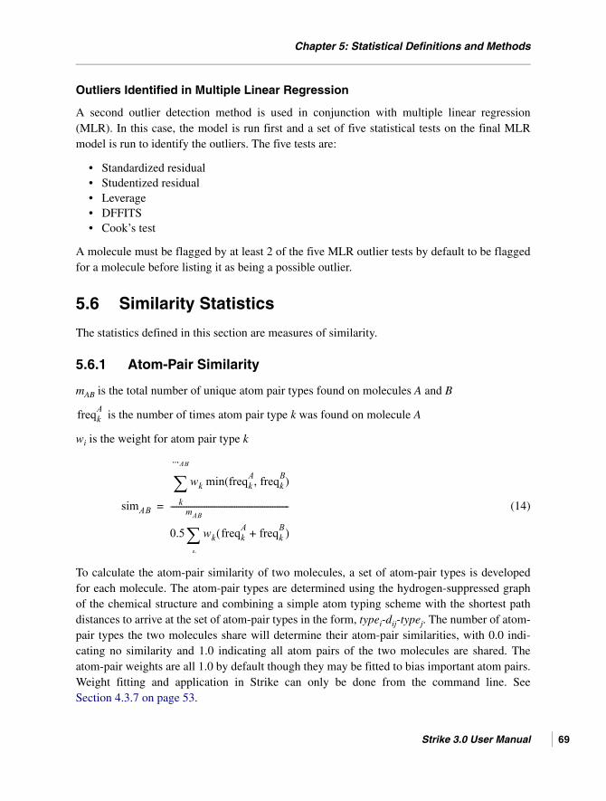
Chapter 5: Statistical Definitions and Methods
Outliers Identified in Multiple Linear Regression
A second outlier detection method is used in conjunction with multiple linear regression(MLR). In this case, the model is run first and a set of five statistical tests on the final MLRmodel is run to identify the outliers. The five tests are:
• Standardized residual• Studentized residual• Leverage• DFFITS• Cook’s test
A molecule must be flagged by at least 2 of the five MLR outlier tests by default to be flaggedfor a molecule before listing it as being a possible outlier.
5.6 Similarity Statistics
The statistics defined in this section are measures of similarity.
5.6.1 Atom-Pair Similarity
mAB is the total number of unique atom pair types found on molecules A and B
is the number of times atom pair type k was found on molecule A
wi is the weight for atom pair type k
(14)
To calculate the atom-pair similarity of two molecules, a set of atom-pair types is developedfor each molecule. The atom-pair types are determined using the hydrogen-suppressed graphof the chemical structure and combining a simple atom typing scheme with the shortest pathdistances to arrive at the set of atom-pair types in the form, typei-dij-typej. The number of atom-pair types the two molecules share will determine their atom-pair similarities, with 0.0 indi-cating no similarity and 1.0 indicating all atom pairs of the two molecules are shared. Theatom-pair weights are all 1.0 by default though they may be fitted to bias important atom pairs.Weight fitting and application in Strike can only be done from the command line. SeeSection 4.3.7 on page 53.
freqkA
simAB
wk min freqkA freqk
B,( )
k
mAB
0.5 wk freqkA freqk
B+( )
k
mAB
-----------------------------------------------------------=
Strike 3.0 User Manual 69

Chapter 5: Statistical Definitions and Methods
70
5.6.2 Similarity Measures in Descriptor Space
The four quantities defined here are measures of distance in descriptor space.
Manhattan Distance
(15)
The Manhattan distance metric, also known as the city-block distance, is a measure of the sumof geometric distances between points measured along axes at right angles. The distance beingmeasured is summed over all variables. Put another way, the distance is calculated between alldescriptors for a molecule and the probe value for each of those descriptors. For descriptorsimilarities, the probe value for each descriptor is the mean of the values of each probe mole-cule for that descriptor. Different weights for each descriptor, wi, may be included only incommand-line Strike calculations, otherwise all weights have the value of one. A value of zeroindicates the probe molecule and test molecules are identical.
Euclidian Squared Distance
(16)
The Euclidean squared distance metric is a measure of the sum of geometric distances betweenpoints. The distance being measured is summed over all variables. Put another way, thedistance is calculated between all descriptors for a molecule and the probe value for each ofthose descriptors. For descriptor similarities, the probe value for each descriptor is the mean ofthe values of each probe molecule for that descriptor. Different weights for each descriptor, wi,may be included only in backend Strike calculations, otherwise all weights have the value ofone. A value of zero indicates the probe molecule and test molecules are identical.
Euclidian Distance
The Euclidean distance is the square root of the expression in Equation (16).
Tanimoto Similarity
(17)
dist wi xi xiprobe–
i=
dist wi xi xiprobe–( )2
i=
dist
xixiprobe
i
xixii xiprobexiprobe
i xixiprobe
i–+
----------------------------------------------------------------------------------------=
Schrödinger Software Release 2015-2

Chapter 5: Statistical Definitions and Methods
The Tanimoto distance metric is a normalized measure of the similarity in descriptor spacebetween a test molecule and a probe molecule. Similarities lie between one and zero with avalue of one indicating identical molecules and a value of zero indicating completely dissimilarmolecules.
5.7 References
1. Pearlman, D. A.; Charifson, P. S. J. Med. Chem. 2001, 44, 3417. Note that the inequali-ties in eq. 5 should be inverted.
Strike 3.0 User Manual 71

72
Schrödinger Software Release 2015-2
Strike User Manual
Getting Help
Information about Schrödinger software is available in two main places:
• The docs folder (directory) of your software installation, which contains HTML andPDF documentation. Index pages are available in this folder.
• The Schrödinger web site, http://www.schrodinger.com/, In particular, you can use theKnowledge Base, http://www.schrodinger.com/kb, to find current information on a rangeof topics, and the Known Issues page, http://www.schrodinger.com/knownissues, to findinformation on software issues.
Finding Information in Maestro
Maestro provides access to nearly all the information available on Schrödinger software.
To get information:
• Pause the pointer over a GUI feature (button, menu item, menu, ...). In the main window,information is displayed in the Auto-Help text box, which is located at the foot of themain window, or in a tooltip. In other panels, information is displayed in a tooltip.
If the tooltip does not appear within a second, check that Show tooltips is selected underGeneral → Appearance in the Preferences panel, which you can open with CTRL+, (,).Not all features have tooltips.
• Click the Help button in the lower right corner of a panel or press F1, for informationabout a panel or the tab that is displayed in a panel. The help topic is displayed in the Help
panel. The button may have text or an icon:
• Choose Help → Online Help or press CTRL+H (H) to open the default help topic.
• When help is displayed in the Help panel, use the navigation links in the help topic orsearch the help.
• Choose Help → Documentation Index, to open a page that has links to all the documents.Click a link to open the document.
Strike 3.0 User Manual 73

Getting Help
74
• Choose Help → Search Manuals to search the manuals. The search tab in Adobe Readeropens, and you can search across all the PDF documents. You must have Adobe Readerinstalled to use this feature.
For information on:
• Problems and solutions: choose Help → Knowledge Base or Help → Known Issues →product.
• New software features: choose Help → New Features.
• Python scripting: choose Help → Python Module Overview.
• Utility programs: choose Help → About Utilities.
• Keyboard shortcuts: choose Help → Keyboard Shortcuts.
• Installation and licensing: see the Installation Guide.
• Running and managing jobs: see the Job Control Guide.
• Using Maestro: see the Maestro User Manual.
• Maestro commands: see the Maestro Command Reference Manual.
Contacting Technical Support
If you have questions that are not answered from any of the above sources, contact Schrödingerusing the information below.
Web: http://www.schrodinger.com/supportcenter E-mail: [email protected]: Schrödinger, 101 SW Main Street, Suite 1300, Portland, OR 97204Phone: +1 888 891-4701 (USA, 8am – 8pm Eastern Time)
+49 621 438-55173 (Europe, 9am – 5pm Central European Time)Fax: +1 503 299-4532 (USA, Portland office)FTP: ftp://ftp.schrodinger.com
Generally, using the web form is best because you can add machine output and upload files, ifnecessary. You will need to include the following information:
• All relevant user input and machine output• Strike purchaser (company, research institution, or individual)• Primary Strike user• Installation, licensing, and machine information as described below.
Schrödinger Software Release 2015-2

Getting Help
Gathering Information for Technical Support
The instructions below describe how to gather the required machine, licensing, and installationinformation, and any other job-related or failure-related information, to send to technicalsupport. Where the instructions depend on the profile used for Maestro, the profile is indicated.
For general enquiries or problems:
1. Open the Diagnostics panel.
• Maestro: Help → Diagnostics • Windows: Start → All Programs → Schrodinger-2015-2 → Diagnostics • Mac: Applications → Schrodinger2015-2 → Diagnostics • Command line: $SCHRODINGER/diagnostics
2. When the diagnostics have run, click Technical Support.
A dialog box opens, with instructions. You can highlight and copy the name of the file.
3. Upload the file specified in the dialog box to the support web form.
If you have already submitted a support request, use the upload link in the email responsefrom Schrödinger to upload the file. If you need to submit a new request, you can uploadthe file when you fill in the form.
If your job failed:
1. Open the Monitor panel, using the instructions for your profile as given below:
• Maestro/Jaguar/Elements: Tasks → Monitor Jobs• BioLuminate/MaterialsScience: Tasks → Job Monitor
2. Select the failed job in the table, and click Postmortem.
The Postmortem panel opens.
3. If your data is not sensitive and you can send it, select Include structures and deselectAutomatically obfuscate path names.
4. Click Create.
An archive file is created, and an information dialog box with the name and location ofthe file opens. You can highlight and copy the name of the file.
5. Upload the file specified in the dialog box to the support web form.
If you have already submitted a support request, use the upload link in the email responsefrom Schrödinger to upload the file. If you need to submit a new request, you can uploadthe file when you fill in the form.
Strike 3.0 User Manual 75

Getting Help
76
6. Copy and paste any log messages from the window used to start the interface or the jobinto the web form (or an e-mail message), or attach them as a file.
• Windows: Right-click in the window and choose Select All, then press ENTER tocopy the text.
• Mac: Start the Console application (Applications → Utilities), filter on the applica-tion that you used to start the job (Maestro, BioLuminate, Elements), copy the text.
If Maestro failed:
1. Open the Diagnostics panel.
• Windows: Start → All Programs → Schrodinger-2015-2 → Diagnostics • Mac: Applications → SchrodingerSuite2015-2 → Diagnostics • Linux/command line: $SCHRODINGER/diagnostics
2. When the diagnostics have run, click Technical Support.
A dialog box opens, with instructions. You can highlight and copy the name of the file.
3. Upload the file specified in the dialog box to the support web form.
If you have already submitted a support request, use the upload link in the email responsefrom Schrödinger to upload the file. If you need to submit a new request, you can uploadthe file when you fill in the form.
4. Upload the error files to the support web form.
The files should be in the following location:
• Windows: %LOCALAPPDATA%\Schrodinger\appcrash (Choose Start → Run and paste this location into the Open text box.)Attach maestro_error_pid.txt and maestro.exe_pid_timestamp.dmp.
• Mac: $HOME/Library/Logs/CrashReporter (Go → Home → Library → Logs → CrashReporter)Attach maestro_error_pid.txt and maestro_timestamp_machinename.crash.
• Linux: $HOME/.schrodinger/appcrash Attach maestro_error_pid.txt and crash_report_timestamp_pid.txt.
If a Maestro panel failed to open:
1. Copy the text in the dialog box that opens.
2. Paste the text into the support web form.
Schrödinger Software Release 2015-2

Index
Aactive ligands, extracting................................... 27activity property .......................................... 12, 65atom-pair connectivity .......................... 24, 45, 69atom-pair similarity........................................... 69
maximum.................................................... 27mean ........................................................... 27
atom-pair types ................................................. 69atom-pair weights ............................................. 69
Bbivariate statistics.................................. 19, 20, 62Build QSAR Model panel................................. 40
CCalculate Similarity panel................................. 45central tendency (of a variable)......................... 59city-block distance ............................................ 70conventions, document..................................... viicorrelation coefficient ....................................... 62correlation matrix.............................................. 62covariance ......................................................... 62cross validation ................................................. 67
Ddata reduction.................................................... 22database
for calculating similarities .......................... 26seeding........................................................ 26
dependent descriptor ......................................... 65dependent variable ...................................... 12, 65descriptor space........................................... 45, 70descriptors ........................................................... 8
from ligparse ............................................ 9from QikProp................................................ 9weight in similarity evaluation ................... 45
directoryinstallation .................................................... 1Maestro working........................................... 2
distanceEuclidean .................................................... 70in descriptor space ...................................... 70Manhattan ................................................... 70Tanimoto..................................................... 71
Eeigenvalue, PCA model .................................... 21environment variable
SCHRODINGER .............................................. 1Euclidean distance ............................................ 70Euclidean similarity .......................................... 29Euclidean squared distance............................... 70Euclidean squared similarity............................. 29extracting actives .............................................. 27
FFactor Analysis panel.................................. 46, 47Fisher skewness ................................................ 61F-statistic........................................................... 68
Iindependent descriptors .................................... 65independent variables ................................. 12, 65input file............................................................ 49installation........................................................... 5
KKendall tau........................................................ 64kurtosis.............................................................. 62
Lleave-group-out (LGO) validation .................... 67leave-n-out validation ....................................... 67lgoCycles .......................................................... 67lgoPercent ......................................................... 67ligparse utility................................................. 9loadings plot, factor analysis ............................ 46Local Correlation Integral Outlier (LOCI)
Detection........................................................ 68
MManhattan distance ........................................... 70Manhattan similarity ......................................... 29Max AP Similarity ............................................ 27maximum atom-pair similarity ................... 27, 28mean (of variable x) .......................................... 59mean absolute deviation.................................... 60Mean AP Similarity .......................................... 27mean atom-pair similarity................................. 28
Strike 3.0 User Manual 77
78
Index
mean squared deviation..................................... 61median............................................................... 59MLR—see multiple linear regression (MLR)mode.................................................................. 60molecular properties ........................................... 8
from QikProp................................................ 9multiple linear regression (MLR)
definition..................................................... 67keyword ...................................................... 52optimal subset............................................. 42selecting method......................................... 42tutorial example .......................................... 23
Nn-factor predictor ........................................ 14, 21normal distribution...................................... 61, 62number of data points ....................................... 59
Ooptimal set of descriptors ............................ 23, 42optimal subset ................................................... 23outlier detection ................................................ 68output file, model-building job ......................... 43
Ppartial least squares (PLS)
definition..................................................... 66keyword ...................................................... 52selecting method......................................... 41tutorial example .......................................... 11
PCA—see principal component analysis (PCA)Pearson r ........................................................... 63PLS—see partial least squares (PLS)Predict based on QSAR Model panel ............... 43Predicted Activity property............................... 13predicted property ............................................. 18predicted values ................................................ 18prediction, running............................................ 44predictive index................................................. 64predictor ............................................................ 13principal component analysis (PCA)
definition..................................................... 66eigenvalue ................................................... 21factor analysis ............................................. 45keyword ...................................................... 52
selecting method......................................... 41tutorial example.......................................... 21
product installation ........................................... 74Project Table ....................................................... 8properties ............................................................ 8
from ligparse ............................................ 9p-value .............................................................. 68
QQikProp............................................................... 9QSAR model
building................................................. 11, 33viewing results............................................ 16
q-squared..................................................... 67, 68
Rrandom selection................................................. 9regression methods ........................................... 65response variable............................................... 65results table ....................................................... 13root mean squared deviation ............................. 61rotatable bonds.................................................. 12r-squared ........................................................... 63
Sscatter plot......................................................... 63Schrödinger contact information ...................... 74scores plot, factor analysis ................................ 45seeding database ............................................... 26similarity
atom-pair ........................................ 24, 45, 69descriptor space .................................... 45, 70descriptor weights ...................................... 45maximum atom-pair ................................... 28mean atom-pair..................................... 27, 28tutorial example.......................................... 24
skewness ........................................................... 61Spearman rho .................................................... 63standard deviation ............................................. 60statistics
bivariate .......................................... 19, 48, 62univariate ........................................ 19, 48, 59
statistics script................................................... 19strike command............................................. 49Strike input file ................................................. 49
Schrödinger Software Release 2015-2

Index
TTanimoto distance ............................................. 71Tanimoto similarity ........................................... 29test set ................................................................. 9
creating ................................................. 17, 35total variance..................................................... 22training set........................................................... 9
Uunivariate statistics................................ 19, 20, 59
Vvalidation .................................................... 17, 35variance............................................................. 60
total............................................................. 22View QSAR Model dialog box......................... 16
Wweights, of descriptors in similarity evaluation 45
Strike 3.0 User Manual 79

80
Schrödinger Software Release 2015-2

120 West 45th Street 17th FloorNew York, NY 10036
101 SW Main StreetSuite 1300Portland, OR 97204
245 First StreetRiverview II, 18th FloorCambridge, MA 02142
8910 University Center LaneSuite 270San Diego, CA 92122
155 Gibbs StSuite 430Rockville, MD 20850-0353
Dynamostraße 13D-68165 MannheimGermany
Zeppelinstraße 73D-81669 MünchenGermany
Potsdamer Platz 11D-10785 BerlinGermany
Quatro HouseFrimley RoadCamberley GU16 7ERUnited Kingdom
8F Pacific Century Place1-11-1 MarunouchiChiyoda-ku, Tokyo 100-6208Japan
No. 102, 4th Block3rd Main Road, 3rd StageSharada ColonyBasaveshwaranagarBangalore 560079, India
SCHRÖDINGER ®