Available online at www.sciencedirect.com

www.elsevier.com/locate/solener

ScienceDirect

Solar Energy 108 (2014) 447–459

Streamline-based method for intra-day solar forecasting throughremote sensing

Lukas Nonnenmacher, Carlos F.M. Coimbra ⇑

Department of Mechanical and Aerospace Engineering, Jacobs School of Engineering, Center for Renewable Resource Integration and Center for

Energy Research, University of California, 9500 Gilman Drive, La Jolla, CA 92093, USA

Received 25 March 2014; received in revised form 30 July 2014; accepted 31 July 2014

Communicated by: Associate Editor Frank Vignola

Abstract

This work presents an enhanced deterministic solar irradiance forecasting approach that relies on satellite images and ground mea-surements as inputs. The proposed method is based on a ground-truth improved satellite-to-irradiance model for the prediction of globalhorizontal irradiance (GHI). This approach relies on cloud tracking and advection with an optical flow algorithm. The application of theoptical flow algorithm between two consecutive satellite image frames allows for the calculation of a vector field covering each pixel in thesatellite image. This cloud motion vector (CMV ) field determines the streamline passing through the location of interest. The estimatedcloud advection along the quasi-steady streamline to the location of interest is than computed, and this information is translated into anirradiance forecast for the location of interest. In order to reduce the error associated with a linear satellite-to-irradiance model, a novelapproach employing ground measurements is proposed. Additionally, decision heuristics are identified and implemented to issue a fore-cast based on CMV or persistence, depending on the current sky conditions. The overall method is tested for over 110 days of operational1-, 2- and 3-h ahead GHI forecasts, implemented and evaluated for San Diego, California. The continual forecasting skill of this methodfor the 110 days ranges between 8% and 19% over persistence, depending on the forecast horizon. While previously proposed methodsachieve similar skills, the completely deterministic approach combined with comparably low computation and implementation costsmakes the proposed method suitable for applications with limited availability of data.� 2014 Elsevier Ltd. All rights reserved.

Keywords: Solar forecasting; Remote sensing; Cloud tracking; Optical flow; Global horizontal irradiance

1. Introduction

Solar power is a virtually inexhaustible energy resourcethat is likely to play an increasing role in the future energysupply of most, if not all, societies. While technologicalimprovements enable more efficient and cost effective solarpower generation, the fluctuation of solar irradiance at thesurface of the Earth still constitutes a major obstacle forpower grid integration. Solar forecasting on multiple time

http://dx.doi.org/10.1016/j.solener.2014.07.026

0038-092X/� 2014 Elsevier Ltd. All rights reserved.

⇑ Corresponding author.E-mail address: ccoimbra@ucsd.edu (C.F.M. Coimbra).

horizons is an effective approach to mitigate the adverseeffects of variable solar power generation on the operationand management of the electric grid. A detailed review ofcurrent solar forecasting methods can be found in Inmanet al. (2013). While short term forecasts (intra-hour)became more sophisticated based on recent advances inground based sky-imagery and modeling techniques(Chow et al., 2011; Ghonima et al., 2012; Marquez andCoimbra, 2013a; Dong et al., 2013; Handa et al., 2014),intra-day methods still lack accuracy. Several previousstudies propose and evaluate methods for intra-day fore-casts (Mathiesen and Kleissl, 2011; Marquez et al., 2013).

Nomenclature

ANN artificial neural networkCDF cumulative distribution functionCMV cloud motion vectorCS clear skyDCA Difference Centroid AlgorithmDNI direct normal irradianceErr. Error calculated as Err: ¼ DGHI ¼ GHIGT�

GHIF

GHICS;GT global horizontal irradiance, indices: CS –clear sky, GT – ground truth

GHIM1;M2 global horizontal irradiance, M1, M2 –irradiance Models 1 and 2

GHIkt global horizontal irradiance modeled withkt-persistencedGHI ;GHIF global horizontal irradiance forecasted withthe proposed method

GOES Geostationary Operational EnvironmentalSatellite

Iðx; y; tÞ brightness of pixel at location x, y at time t

Im downloaded satellite imageL geometrical lengthMAE mean absolute errorMBE mean bias errorMFR-7 multi filter radiometerN number of binsNOAA National Oceanic and Atmospheric Admin-

istrationNWP numerical weather prediction

PIV Particle Image VelocimetryRMSE root mean squared errorRTM radiative transfer modelT thresholdUTC Coordinated Universal Time~V average velocity vector of streamlineX probability bina shift parameteri; j summation indiceskt clear-sky indexk; l geometric averaging parametersn linear cloud indexp; q number of pixels in the x- & y-directionpx pixels forecasting skillu velocity in x-direction (horizontal)v velocity in y-direction (vertical)xcor cross correlation�a average albedo imageb cloud fraction imageDt forecast horizond; � penalty function parameters~f streamline vectorg cloud index imagek regularization parameterq pixel intensity, max & min occurring in data

set.S;D spatial and data penalty functions

448 L. Nonnenmacher, C.F.M. Coimbra / Solar Energy 108 (2014) 447–459

However, especially the direct use of satellite images is cur-rently not very common due to difficulties concerning dataavailability, albedo correction, resolution, cloud segmenta-tion and tracking and real time processing of images. Pre-vious methodologies utilizing satellite images for solarforecasting have been proposed by Hammer et al. (1999,2003) and Marquez et al. (2013). This contribution seeksto take advantage of the online near real-time availabilityof processed satellite images derived from the visible chan-nel (0.55–0.75 lm) of the Geostationary Operational Envi-ronmental Satellites West and East (GOES-W andGOES-E) with a resolution of approximately 1 km, com-bined with a fast cloud segmentation algorithm. Two con-secutive frames of cloud index images (gs) are thefoundation for the application of an advanced optical flowalgorithm proposed by Sun et al. (2010), applied to derivecloud motion vectors (CMV ) between two consecutiveframes. This approach also enables the derivation of cloudvelocity. Optical flow was found the most suitableapproach for cloud tracking during this study, while othercloud tracking methods were the topic of several previouspublications (Endlich and Wolf, 1981; Guillot et al.,2012; Escrig et al., 2013). The CMV field and velocities

are utilized to calculate the streamline of the flow fieldreaching the location of interest. This streamline enablesthe identification of an area of pixels most likely to propelto the location of interest. All of these inputs are determin-istic and therefore provide a method that can be appliedwithout any training for every location covered by satelliteimages. This method is heavily based on the performanceof a satellite-to-irradiance model that translates the identi-fied region of cloud intensity values into forecast values ofGHI at the region of interest. In this context, a ground mea-surement enhanced semi-empirical satellite-to-irradiancemodel has been developed.

This work is divided into two main parts, the satellite-to-irradiance model and the forecasting model. Section 2gives an overview of previously proposed methods coveringthe same forecast horizons for GHI and highlights the pur-pose for this study. Section 3 focuses on the processing ofthe satellite images provided by National Oceanic andAtmospheric Administration (NOAA), the applied cloudsegmentation and the satellite-to-irradiance model. Section4 includes the selection of a cloud tracking method, cloudtracking with optical flow and the deterministic solarirradiance forecasting approach. Section 5 contains the

Fig. 1. Schematic of data processing for the satellite-to-irradiance modelbased solar forecasting system.

L. Nonnenmacher, C.F.M. Coimbra / Solar Energy 108 (2014) 447–459 449

evaluation metrics for the satellite-to-irradiance model andfor the forecasts. Results of the overall methodology forthe location of San Diego, California are discussed. Section6 includes conclusions, prospective applications and openresearch questions based on the results.

2. Background

The field of solar irradiance and photovoltaic poweroutput prediction increased rapidly within the last decade.Various previous studies covered (multiple) hour aheadGHI forecasts, based on several different methods. In gen-eral it can be distinguished between statistical, machinelearning, image based and numerical weather prediction(NWP) based methods. Satellite image based forecastsare among the most promising approaches for 1–3h aheadforecasts. An early approach in satellite based solar irradi-ance forecasting was proposed by Hammer et al. (1999)where clouds are segmented from images captured by theMeteosat satellite and tracked based on a statisticalalgorithm. The cloud motion is than extrapolated and pro-spectively advected cloud regions are translated into theforecast by the satellite-to-irradiance model. Lorenz et al.(2007) showed that the forecasting accuracy based onsatellite images outperforms NWP based predictions forforecast horizons up to 4h ahead. Perez et al. (2010) hlfol-lowed this general approach and applied it for images formthe GOES satellites. Based on a evaluation covering sevenlocations, Perez et al. (2010) found that the satellite basedmodel outperforms NWP derived forecasts for up to 5 hahead. Marquez et al. (2013) combined the CMV basedapproach with artificial neural networks (ANNs) tocreate a hybridized forecast. The performance of thehybrid approach is at par or improves previously obtainedresults.

Motivated by the results presented in Hammer et al.(1999), Lorenz et al. (2007) and Perez et al. (2010), this studyproposes an advanced implementation of the previouslyproposed deterministic satellite-based forecasting tech-niques with various crucial refinements that are necessaryto achieve good forecast performance in a highly variableand difficult to predict solar micro-climate. An unrefinedapplication of deterministic, linear cloud advection basedon precise cloud tracking and without the decision heuristicsleads to a negative forecasting skill for the test location inSan Diego. This is partially due to the impact of frequentlyforming inversion layers over the Pacific Ocean.

3. Data processing and satellite-to-irradiance model

Fig. 1 summarizes the data flow in the present work,including the derivation of cloud index images (g) fromsatellite images pre-processed by NOAA. The cloud indeximages are used for the satellite-to-irradiance model andthe forecast model. The forecast model includes cloudtracking based on optical flow to derive the cloud motionvectors (CMVs). The CMVs are used for streamline and

velocity calculations. Both are utilized to identify advectingcloud regions. The last step consists of the validation of themethodology by means of ground telemetry.

3.1. Ground based irradiance measurements

Ground measurements have been obtained at a solarobservatory equipped with a multi-filter radiometer(MFR-7) by the make Yankee Environmental Systems inSan Diego, California. A detailed description of thedeployed solar observatory and the climate characteristicsat the locations are available in Nonnenmacher et al.(2014). This data is considered to represent the groundtruth. Data sets were collected on a 1 min sample rateand averaged to provide 15 min values.

3.2. Satellite images

Relevant satellite images are accessed via NOAA every15 min during daylight times with an automated downloadscript. The time interval of 15 min is chosen since theground truth validation location (San Diego, California)lies in a narrow band where the recorded areas of theGOES-West and GOES-East satellites overlap. Therefore,images are usually available every 15 min. The most recentsatellite images are available online at http://sat.wrh.noaa.gov/satellite/1km/sandiego/vis1san.gif. The period ofstudy ranged from March 2013 to March 2014. The imagesare pre-processed by NOAA. This enables a clear distinc-tion between clouds and Earth surface without additionalcorrection for the changing sun elevation angle duringthe diurnal cycle. The images are downloaded as PortableNetwork Graphics including a superimposed land mask.The land mask lines are replaced by not-a-number valuesbased on their color. These images are used to derive cloud

450 L. Nonnenmacher, C.F.M. Coimbra / Solar Energy 108 (2014) 447–459

segmented images, also called cloud indexed images (gs).Cloud segmentation to derive gs is important for two pur-poses: (1) irradiance modeling at the Earth surface, and (2)computationally optimized cloud motion detection andcloud speed calculations. This step is crucial for the appli-cation of a satellite-to-irradiance model and the differencecentroid algorithm based cloud tracking. It additionallyreduces computation costs for cloud tracking based onoptical flow. The location of the ground based solar obser-vatory in the satellite image has been identified with trian-gulation based on distinct geographical features. Thisestimation has been optimized and verified by applyingthe satellite-to-irradiance model described below for allpixels in a 30 by 30 pixel area by identifying the one withthe best correlation to the ground data. The downloadedsatellite image is cut to a domain size of 200 by 200 pixelswith the location of interest in the center to reduce compu-tation costs. This domain size was chosen empirically basedon the observation that it is very unlikely that clouds fromoutside of this domain are propelled to the location ofinterest within the studied time horizons.

3.3. Cloud segmentation

While the general idea of cloud tracking goes back to thefirst imagery from satellites, cloud extraction by imagesegmentation as part of an automated weather forecastingsystem was introduced much later by Leung and Jordan(1995). To be able to translate a NOAA satellite imagesinto g, only the following two steps out of the originally 6steps mentioned by Leung and Jordan (1995) are necessary:

(1) Template matching to identify pixels showing theground with its region specific albedo. The templatehas been generated from about 150 manually selectedimages from clear days. The average albedo imagecan than be calculated with the equation:

�a ¼ 1

N

XN

i¼1

Imclear; ð1Þ

where �a indicates the derived average ground albedo mapand Imclear stands for the manually selected satellite imageswith no clouds (clear images). If certain regions over thePacific Ocean have not been free of clouds, the cloud cov-ered areas have been replaced with values of cloudlessregions over the ocean. A well known problem in irradi-ance modeling based on satellite images is caused by areaswith snow cover due to irradiance reflectivity similar toclouds. While this is a problem in certain areas and inter-feres with cloud detection, the error introduced by thiseffect is neglected since the areas of occurrence are not inproximity to the areas of interest of this study.

(2) Amplitude thresholding to separate clouds fromground pixels. To filter the noise introduced by themismatch of the average ground albedo template tothe background, the threshold filter can be setempirically:

gx;y ¼gx;y ¼ 0 if jðImx;y � �ax;yÞj 6 T ;

gx;y ¼ Imx;y if jðImx;y � �ax;yÞj > T ;

(ð2Þ

where g represents the derived cloud indexed image, Im

stands for the latest available satellite image pre-processedby NOAA and T is the applied threshold filter. For thisstudy, T ¼ 3 has been chosen. As mentioned above, �ax;y

indicates pixel intensity values from the average albedoimage at the x- and y-location.

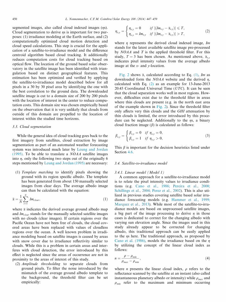
Fig. 2 shows �a, calculated according to Eq. (1), Im asdownloaded form the NOAA website and the derived g,calculated with Eq. (2) as an example for 13-June-201320:45 Coordinated Universal Time (UTC). It can be seenthat the cloud separation works well in most regions. How-ever, difficulties exist due to the threshold filter in areaswhere thin clouds are present (e.g. in the north east areaof the example shown in Fig. 2). Since the threshold filteronly affects very thin clouds and the GHI attenuation bythin clouds is limited, the error introduced by this proce-dure can be neglected. Additionally to the gs, a binarycloud fraction image (b) is calculated as follows:

bx;y ¼bx;y ¼ 0 if gx;y ¼ 0;

bx;y ¼ 1 if gx;y > 0;

(ð3Þ

This b is important for the decision heuristics listed underSection 4.6.

3.4. Satellite-to-irradiance model

3.4.1. Linear model (Model 1)

A common approach for a satellite-to-irradiance modelis to relate the pixel intensity values to irradiance condi-tions (e.g. Cano et al., 1986; Pereira et al., 2000;Schillings et al., 2004; Perez et al., 2002). This is also uti-lized in previous studies covering satellite based solar irra-diance forecasting models (e.g. Hammer et al., 1999;Marquez et al., 2013). While most of the satellite-to-irra-diance models are based on unprocessed satellite images,a big part of the image processing to derive g in thosecases is dedicated to correct for the changing albedo withvarying sun elevation angle. Since the images used in thisstudy already appear to be corrected for changingalbedo, this traditional approach can be easily appliedto the gs here. The traditional approach, as proposed byCano et al. (1986), models the irradiance based on the gby utilizing the concept of the linear cloud index asfollows:

n ¼ q� qmin

qmax � qmin

; ð4Þ

where n presents the linear cloud index, q refers to thereflectance scanned by the satellite at an instant (also calledinstantaneous planetary albedo or intensity) while qmax andqmin refer to the maximum and minimum occurring

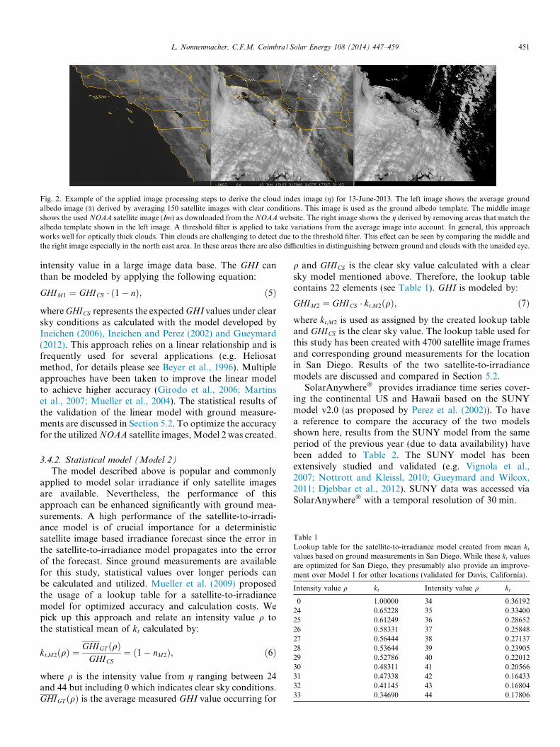
Fig. 2. Example of the applied image processing steps to derive the cloud index image (g) for 13-June-2013. The left image shows the average groundalbedo image (�a) derived by averaging 150 satellite images with clear conditions. This image is used as the ground albedo template. The middle imageshows the used NOAA satellite image (Im) as downloaded from the NOAA website. The right image shows the g derived by removing areas that match thealbedo template shown in the left image. A threshold filter is applied to take variations from the average image into account. In general, this approachworks well for optically thick clouds. Thin clouds are challenging to detect due to the threshold filter. This effect can be seen by comparing the middle andthe right image especially in the north east area. In these areas there are also difficulties in distinguishing between ground and clouds with the unaided eye.

L. Nonnenmacher, C.F.M. Coimbra / Solar Energy 108 (2014) 447–459 451

intensity value in a large image data base. The GHI canthan be modeled by applying the following equation:

GHIM1 ¼ GHICS � ð1� nÞ; ð5Þ

where GHICS represents the expected GHI values under clearsky conditions as calculated with the model developed byIneichen (2006), Ineichen and Perez (2002) and Gueymard(2012). This approach relies on a linear relationship and isfrequently used for several applications (e.g. Heliosatmethod, for details please see Beyer et al., 1996). Multipleapproaches have been taken to improve the linear modelto achieve higher accuracy (Girodo et al., 2006; Martinset al., 2007; Mueller et al., 2004). The statistical results ofthe validation of the linear model with ground measure-ments are discussed in Section 5.2. To optimize the accuracyfor the utilized NOAA satellite images, Model 2 was created.

Table 1Lookup table for the satellite-to-irradiance model created from mean kt

values based on ground measurements in San Diego. While these kt valuesare optimized for San Diego, they presumably also provide an improve-ment over Model 1 for other locations (validated for Davis, California).

Intensity value q kt Intensity value q kt

0 1.00000 34 0.3619224 0.65228 35 0.3340025 0.61249 36 0.2865226 0.58331 37 0.2584827 0.56444 38 0.2713728 0.53644 39 0.2390529 0.52786 40 0.2201230 0.48311 41 0.2056631 0.47338 42 0.1643332 0.41145 43 0.1680433 0.34690 44 0.17806

3.4.2. Statistical model (Model 2)

The model described above is popular and commonlyapplied to model solar irradiance if only satellite imagesare available. Nevertheless, the performance of thisapproach can be enhanced significantly with ground mea-surements. A high performance of the satellite-to-irradi-ance model is of crucial importance for a deterministicsatellite image based irradiance forecast since the error inthe satellite-to-irradiance model propagates into the errorof the forecast. Since ground measurements are availablefor this study, statistical values over longer periods canbe calculated and utilized. Mueller et al. (2009) proposedthe usage of a lookup table for a satellite-to-irradiancemodel for optimized accuracy and calculation costs. Wepick up this approach and relate an intensity value q tothe statistical mean of kt calculated by:

kt;M2ðqÞ ¼GHIGT ðqÞ

GHICS¼ ð1� nM2Þ; ð6Þ

where q is the intensity value from g ranging between 24and 44 but including 0 which indicates clear sky conditions.GHIGT ðqÞ is the average measured GHI value occurring for

q and GHICS is the clear sky value calculated with a clearsky model mentioned above. Therefore, the lookup tablecontains 22 elements (see Table 1). GHI is modeled by:

GHIM2 ¼ GHICS � kt;M2ðqÞ; ð7Þwhere kt;M2 is used as assigned by the created lookup tableand GHICS is the clear sky value. The lookup table used forthis study has been created with 4700 satellite image framesand corresponding ground measurements for the locationin San Diego. Results of the two satellite-to-irradiancemodels are discussed and compared in Section 5.2.

SolarAnywhere� provides irradiance time series cover-ing the continental US and Hawaii based on the SUNYmodel v2.0 (as proposed by Perez et al. (2002)). To havea reference to compare the accuracy of the two modelsshown here, results from the SUNY model from the sameperiod of the previous year (due to data availability) havebeen added to Table 2. The SUNY model has beenextensively studied and validated (e.g. Vignola et al.,2007; Nottrott and Kleissl, 2010; Gueymard and Wilcox,2011; Djebbar et al., 2012). SUNY data was accessed viaSolarAnywhere� with a temporal resolution of 30 min.

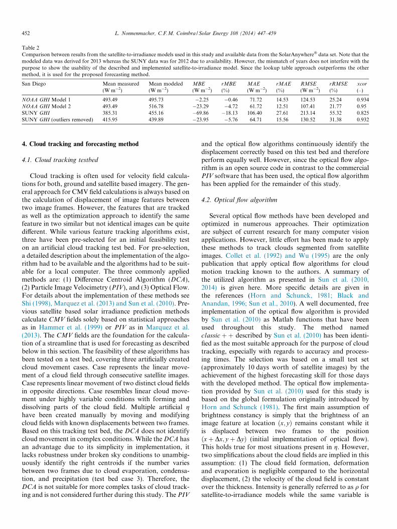
Table 2Comparison between results from the satellite-to-irradiance models used in this study and available data from the SolarAnywhere� data set. Note that themodeled data was derived for 2013 whereas the SUNY data was for 2012 due to availability. However, the mismatch of years does not interfere with thepurpose to show the usability of the described and implemented satellite-to-irradiance model. Since the lookup table approach outperforms the othermethod, it is used for the proposed forecasting method.

San Diego Mean measured(W m�2)

Mean modeled(W m�2)

MBE

(W m�2)rMBE

(%)MAE

(W m�2)rMAE

(%)RMSE

(W m�2)rRMSE

(%)xcor

(–)

NOAA GHI Model 1 493.49 495.73 �2.25 �0.46 71.72 14.53 124.53 25.24 0.934NOAA GHI Model 2 493.49 516.78 �23.29 �4.72 61.72 12.51 107.41 21.77 0.95SUNY GHI 385.31 455.16 �69.86 �18.13 106.40 27.61 213.14 55.32 0.825SUNY GHI (outliers removed) 415.95 439.89 �23.95 �5.76 64.71 15.56 130.52 31.38 0.932

452 L. Nonnenmacher, C.F.M. Coimbra / Solar Energy 108 (2014) 447–459

4. Cloud tracking and forecasting method

4.1. Cloud tracking testbed

Cloud tracking is often used for velocity field calcula-tions for both, ground and satellite based imagery. The gen-eral approach for CMV field calculations is always based onthe calculation of displacement of image features betweentwo image frames. However, the features that are trackedas well as the optimization approach to identify the samefeature in two similar but not identical images can be quitedifferent. While various feature tracking algorithms exist,three have been pre-selected for an initial feasibility teston an artificial cloud tracking test bed. For pre-selection,a detailed description about the implementation of the algo-rithm had to be available and the algorithms had to be suit-able for a local computer. The three commonly appliedmethods are: (1) Difference Centroid Algorithm (DCA),(2) Particle Image Velocimetry (PIV), and (3) Optical Flow.For details about the implementation of these methods seeShi (1998), Marquez et al. (2013) and Sun et al. (2010). Pre-vious satellite based solar irradiance prediction methodscalculate CMV fields solely based on statistical approachesas in Hammer et al. (1999) or PIV as in Marquez et al.(2013). The CMV fields are the foundation for the calcula-tion of a streamline that is used for forecasting as describedbelow in this section. The feasibility of these algorithms hasbeen tested on a test bed, covering three artificially createdcloud movement cases. Case represents the linear move-ment of a cloud field through consecutive satellite images.Case represents linear movement of two distinct cloud fieldsin opposite directions. Case resembles linear cloud move-ment under highly variable conditions with forming anddissolving parts of the cloud field. Multiple artificial ghave been created manually by moving and modifyingcloud fields with known displacements between two frames.Based on this tracking test bed, the DCA does not identifycloud movement in complex conditions. While the DCA hasan advantage due to its simplicity in implementation, itlacks robustness under broken sky conditions to unambig-uously identify the right centroids if the number variesbetween two frames due to cloud evaporation, condensa-tion, and precipitation (test bed case 3). Therefore, theDCA is not suitable for more complex tasks of cloud track-ing and is not considered further during this study. The PIV

and the optical flow algorithms continuously identify thedisplacement correctly based on this test bed and thereforeperform equally well. However, since the optical flow algo-rithm is an open source code in contrast to the commercialPIV software that has been used, the optical flow algorithmhas been applied for the remainder of this study.

4.2. Optical flow algorithm

Several optical flow methods have been developed andoptimized in numerous approaches. Their optimizationare subject of current research for many computer visionapplications. However, little effort has been made to applythese methods to track clouds segmented from satelliteimages. Collet et al. (1992) and Wu (1995) are the onlypublication that apply optical flow algorithms for cloudmotion tracking known to the authors. A summary ofthe utilized algorithm as presented in Sun et al. (2010,2014) is given here. More specific details are given inthe references (Horn and Schunck, 1981; Black andAnandan, 1996; Sun et al., 2010). A well documented, freeimplementation of the optical flow algorithm is providedby Sun et al. (2010) as Matlab functions that have beenused throughout this study. The method namedclassicþþ described by Sun et al. (2010) has been identi-fied as the most suitable approach for the purpose of cloudtracking, especially with regards to accuracy and process-ing times. The selection was based on a small test set(approximately 10 days worth of satellite images) by theachievement of the highest forecasting skill for those dayswith the developed method. The optical flow implementa-tion provided by Sun et al. (2010) used for this study isbased on the global formulation originally introduced byHorn and Schunck (1981). The first main assumption ofbrightness constancy is simply that the brightness of animage feature at location ðx; yÞ remains constant while itis displaced between two frames to the positionðxþ Dx; y þ DyÞ (initial implementation of optical flow).This holds true for most situations present in g. However,two simplifications about the cloud fields are implied in thisassumption: (1) The cloud field formation, deformationand evaporation is negligible compared to the horizontaldisplacement, (2) the velocity of the cloud field is constantover the thickness. Intensity is generally referred to as q forsatellite-to-irradiance models while the same variable is

L. Nonnenmacher, C.F.M. Coimbra / Solar Energy 108 (2014) 447–459 453

generally refereed to as brightness (I) in computer vision.To obey conventional nomenclature, we use I for thebrightness when referring to optical flow calculations. Wecan write the following equation:

Iðx; y; tÞ ¼ Iðxþ uDt; y þ vDt; t þ DtÞ; ð8Þ

where I indicates the brightness at the location ðx; yÞ at timet of the g. Dt is the time passing between two consecutivelyavailable gs. Intensity values will be referred to as I1 (firstimage) and I2 (consecutive image) from now on. This isthe basic equation defining the general approach to thedetection of optical flow. For this equation, a set of addi-tional constraints are needed to allow for solution. Theseadditional constraints can be derived via several ways,e.g. correlation methods, gradient methods or regressionmethods (Black and Anandan, 1996). According to Sunet al. (2010) the spatially discrete classical optical flowobjective function can be written as:

F ðu; vÞ ¼X

x;y

.DðI1ðx; yÞ � I2ðxþ ux;y ; y þ vx;yÞÞ�

þ k½.Sðux;y � uxþ1;yÞ þ .Sðux;y � ux;yþ1Þþ.Sðvx;y � vxþ1;yÞ þ .Sðvx;y � vx;yþ1Þ�

�; ð9Þ

where F refers to the calculated flow field with the u and v

velocities in the x- and y-direction. The variables .S and .D

refer to the spatial and data penalty functions. The penaltyfunction . combines the data term (subscript D) thatassumes constant image properties with the spatial term(subscript S) that models how flow is expected to varyacross the image. The combination of these terms is opti-mized with an objective function. k is the regularizationparameter. Based on the study of Sun et al. (2010), k ¼ 3was used based on the performance on the Middlebury test.As suggested in Bruhn et al. (2005), a Charbonnier penaltyfunction is used as:

.ðxÞ ¼ ðx2 þ �2Þ0:45; ð10Þ

for both, data and spatial penalty in the x-direction(y-direction similarly), � is the variation parameter. Basedon the used implementation � ¼ 0:001.

4.3. Streamline and velocity

A key part of the deterministic forecast is based on thecalculation of the streamline that passes through San Diegoin the CMV field. Streamlines in the 2-dimensional spaceare calculated by definition as:

dxu¼ dy

v; ð11Þ

where dx and dy are line elements of the streamline of arc

length. The local velocity in the x and y direction are indi-cated by u and v and given by the calculated CMV field.After this application, we obtain a streamline passingthrough the location of interest as a vector of the from~f ¼ ðx1; . . . ; xn; y1; . . . ; ynÞ. It is straight forward to only

use the upstream part of the streamline. After the stream-line has been obtained, the average velocity vector for thestreamline between two frames can be calculated by:

~V ¼ 1

N

XN

i¼1

ðui; viÞ ð12Þ

where u and v are indicating the x- and y-velocities of the

CMV field covered by the streamline ~f (i 2~f). This leavesus with a speed in vector form derived in the unit pixelper frame (px=frame). The magnitude of the velocity can

be obtained by taking j~V j rounded to the next integer.From here on, we know the directions of cloud flow as wellas the associated velocity.

4.4. Forecasting model

After the calculation of the streamline and the associ-ated average velocity, a forecast can be issued under theassumption that the identified CMV field between gt andgtþ1 will persist and that the velocity ~V can be extrapolatedto the time horizon of interest (frozen cloud assumption).Based on these parameters, the conditions likely to propelto the location of interest in the time horizon of interestcan be identified (see Fig. 3 for an example). The cloudconditions over this region can be translated to an irradi-ance forecast based on the satellite-to-irradiance modeldiscussed above. Therefore, the forecast can be issuedaccording to the following:

qt ¼ gð~fðxn; ynÞÞ; ð13Þwhere xn and yn are the vector elements of the streamlinethat are presumably propelling to the location of the fore-cast. This leaves us with an intensity value qt that canbe used for the satellite to irradiance model. To identifythe pixel on the streamline that is likely to be propelledto the location of interest, we have to define the shiftparameter a ¼ 1þ jvj � Dt. In this study, predicted values

will be superimposed with a �-symbol, e.g. dGHI . Since thepreviously mentioned assumptions are a simplification fora significantly more complex system, the forecasting skillcan be enhanced by taking surrounding pixels into account.The basic function for a spatial averaging filter for a regionof p � q pixels is given by Nakariyakul (2013) as:

gðx; yÞ ¼ 1

p � qX

k

Xl

f ðx� k; y � lÞ ð14Þ

where f ðx; yÞ is the input region and gðx; yÞ is the averagedoutput region, while k and l represent the size of the aver-aging window in the x- and y-direction, respectively. Theaveraging area was chosen to be square (k ¼ l) and wasoptimized with the development set. It has been found tobe k ¼ 8 pixels for the 1h-ahead forecast, k ¼ 10 pixelsfor the 2h ahead forecast and k ¼ 11 pixels for the 3h aheadforecast. This averaging over a larger area leads to theeffect that not only intensity values in the range 22–44can occur but also other values. For this purpose, a lookup

454 L. Nonnenmacher, C.F.M. Coimbra / Solar Energy 108 (2014) 447–459

table with this range as been created according to Eq. (6).Since in our study, the input region consists of an intensityimage g and the output region is supposed to be only oneaverage intensity value q, we can insert Eq. (13) in (14)to obtain Eq. (15)as follows:

�qt ¼1

N

XL

i¼�L

XL

j¼�L

gð~fðxaÞ þ i;~fðyaÞ þ jÞ: ð15Þ

The forecast can then be issued by applying:dGHI tþDt ¼ GHICS;tþDt � ktð �qtÞ: ð16Þ

Based on the results obtained above (see Table 2), Model 2is used as the satellite-to-irradiance model translating theobtained intensity g from Eq. (15) to ktð �qtÞ.

4.5. Persistence forecast

As a baseline forecast and an alternative when thestreamline based forecast cannot be issued (e.g. due to cor-rupt satellite images), the persistence forecast is defined as:dGHI kt;tþDt ¼ GHICS;tþDt � kt;t; ð17Þ

where GHICS;t refers to the GHI under clear conditions atthe time of the forecast and kt is the calculated clear-skyindex with the latest available values. This forecast willbe called kt-persistence in this study. This model is alsoused as a forecasting reference to evaluate the forecastingskill as discussed in Section 5.3.

4.6. Decision heuristics

An essential step for the operational applicability of aforecasting model is the pre-classification of days to allowan automatized switch into different cloud cover modes.The heuristics to guarantee that the applied method isapplicable for the existing and upcoming atmospheric con-ditions are implemented as follows:

4.6.1. Cloudless domain

In case that the domain of interest is free of clouds, itcan be assumed that the clearness persists until clouds startto form or advect into the domain. The domain is assumedas clear if the number of cloudy pixels in the area is lowerthan 5%. In this case, the model switches to kt-persistence.This threshold has been chosen empirically to allow fornoise in the cloud identification process. The size of theinput satellite image is a window of 200 by 200 pixels.Therefore, if

Px

Pyb < 2000, the issued forecast is solely

based on the clear sky model and the latest ground kt value(kt-persistence).

4.6.2. Negligible cloud movement speed

If the cloud movement is below 3 pixels per frame(j~V j < 3px=frame), the forecast algorithm also switches tokt-persistence by extrapolating the latest available kt valueto the forecast horizon of interest. This assumption can

be made since it is very unlikely that clouds will be pro-pelled in or out of the region of interest. These two assump-tions have been found highly reliable in the implementationof operational forecasts.

4.7. Short streamline

It can occur that a calculated streamline~f is shorter thanthe shift parameter (a) depending on the CMV field. In thatcase, the last available value of the streamline vector ~f istaken as the identified pixel. This is only an approximation,nevertheless it is useful to continuously issue a forecast.

4.8. Data quality control

Occasionally, satellite images were not online, notdownloaded correctly or the downloaded image was cor-rupt. Additionally, the stream of ground measurementscould be interrupted by instrument malfunction, connectiv-ity issues or maintenance work. If the issues with the inputdata could be detected, the forecasting system automati-cally switches to the kt-persistence model. In this way, aforecast is continuously issued while the achieved skill forthose days is zero. Approximately 10% of all days usedfor this study contained corrupt data of some sort andtherefore have been excluded from the evaluation of theforecasting capabilities.

5. Model evaluations

To evaluate the performance of the proposed satellite-to-irradiance and forecasting model, they have been imple-mented for San Diego, California (longitude: 32.88; lati-tude: �117.23). The satellite-to-irradiance model has beenevaluated for 100 days covering a time period from 20-March-2013 to 27-June-2013. The development of the fore-casting method, including the implementation of the men-tioned heuristics, has been done on a data set coveringimages and ground measurements from 13-October-201309:00 Pacific Daylight Time until 15-January-201415:45:00 for a total of 80 days in that period. This set isreferred to as the development set. The method derivedand implemented with the development set was thenapplied to a validation set covering the time period from21-March-2013 09:00 until 07-July-2013 15:45 containing110 days of data. The results obtained with both data setsfor 1h-, 2h- and 3h-ahead forecast horizons are discussedand analyzed in this section. A quantitative and qualitativeerror analysis, including a comparison to the results of pre-viously proposed methods, covering the same forecast hori-zons are presented. The evaluation of the model is based onthe metrics defined below.

5.1. Evaluation metrics

Current research efforts in the solar forecasting fieldhave led to numerous approaches to evaluate the applica-

L. Nonnenmacher, C.F.M. Coimbra / Solar Energy 108 (2014) 447–459 455

bility and compare different forecasting methods. To pro-vide an accurate representation of the capabilities of theforecasting methods proposed in this study, several metricsare used. For a more detailed description about commonways to describe the performance of solar forecasts, referto Marquez and Coimbra (2013b). The error metrics meanbias error (MBE), mean absolute error (MAE), root meansquare error (RMSE) and the cross-correlation (xcor) areused here:

MBE ¼ 1

N

XN

i¼1

ðGHIGT ;i � dGHI iÞ; ð18Þ

MAE ¼ 1

N

XN

i¼1

jGHIGT ;i � dGHI ij; ð19Þ

RMSE ¼ffiffiffiffiffiffiffiffiffiffiffiffiffiffiffiffiffiffiffiffiffiffiffiffiffiffiffiffiffiffiffiffiffiffiffiffiffiffiffiffiffiffiffiffiffiffiffiffiffiffiffiffiffiffi1

N

XN

i¼1ðGHIGT ;i � dGHI iÞ

2r

; ð20Þ

xcor ¼PN

i¼1 ðGHIGT ;i � GHIGT Þ � ðdGHI i � dGHI Þ� �

ffiffiffiffiffiffiffiffiffiffiffiffiffiffiffiffiffiffiffiffiffiffiffiffiffiffiffiffiffiffiffiffiffiffiffiffiffiffiffiffiffiffiffiffiffiffiffiffiffiffiffiffiffiffiffiffiffiffiffiffiffiffiffiffiffiffiffiffiffiffiffiffiffiffiffiffiffiffiffiffiffiffiffiffiffiffiffiffiffiffiffiffiffiffiffiPNi¼1ðGHIGT ;i � GHIGT Þ

2 �PN

i¼1ðdGHI i � dGHI Þ2

r ;

ð21Þ

these statistics are calculated and presented in Tables 2and 3. Additionally to the values calculated in W m�2, itis possible to calculate relative values of the forecast perfor-mance with the average ground truth value as a reference

(GHIGT ). These relative values of the error are indicatedwith a prefixed r. To provide an important evaluation cri-teria to measure the forecast quality and to make resultscomparable to other forecast approaches (e.g. Marquezand Coimbra, 2013b; Chu et al., 2013; Quesada-Ruizet al., 2014), the forecasting skill is calculated as:

s ¼ 1�RMSEcGHI

RMSEkt-pers:: ð22Þ

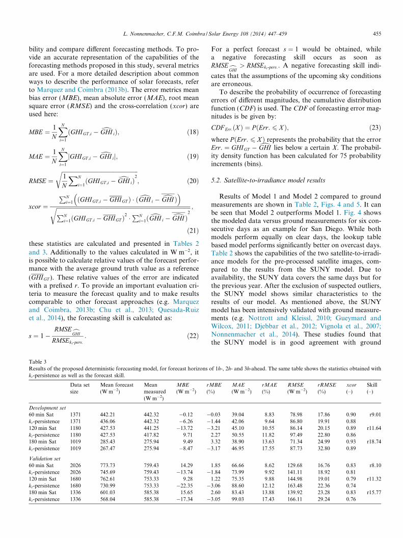
Table 3Results of the proposed deterministic forecasting model, for forecast horizons okt-persistence as well as the forecast skill.

Data setsize

Mean forecast(W m�2)

Meanmeasured(W m�2)

MBE

(W m�2)rM

(%

Development set

60 min Sat 1371 442.21 442.32 �0.12 �kt-persistence 1371 436.06 442.32 �6.26 �120 min Sat 1180 427.53 441.25 �13.72 �kt-persistence 1180 427.53 417.82 9.71180 min Sat 1019 285.43 275.94 9.49kt-persistence 1019 267.47 275.94 �8.47 �

Validation set

60 min Sat 2026 773.73 759.43 14.29kt-persistence 2026 745.69 759.43 �13.74 �120 min Sat 1680 762.61 753.33 9.28kt-persistence 1680 730.99 753.33 �22.35 �180 min Sat 1336 601.03 585.38 15.65kt-persistence 1336 568.04 585.38 �17.34 �

For a perfect forecast s ¼ 1 would be obtained, whilea negative forecasting skill occurs as soon asRMSEcGHI

> RMSEkt-pers:. A negative forecasting skill indi-

cates that the assumptions of the upcoming sky conditionsare erroneous.

To describe the probability of occurrence of forecastingerrors of different magnitudes, the cumulative distributionfunction (CDF) is used. The CDF of forecasting error mag-nitudes is be given by:

CDF Err:ðX Þ ¼ P ðErr: 6 X Þ; ð23Þwhere P ðErr: 6 X Þ represents the probability that the errorErr: ¼ GHIGT � dGHI lies below a certain X. The probabil-ity density function has been calculated for 75 probabilityincrements (bins).

5.2. Satellite-to-irradiance model results

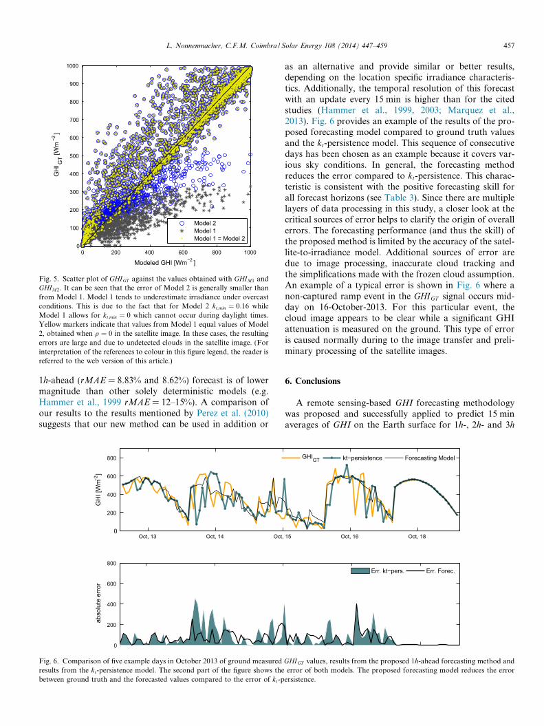
Results of Model 1 and Model 2 compared to groundmeasurements are shown in Table 2, Figs. 4 and 5. It canbe seen that Model 2 outperforms Model 1. Fig. 4 showsthe modeled data versus ground measurements for six con-secutive days as an example for San Diego. While bothmodels perform equally on clear days, the lookup tablebased model performs significantly better on overcast days.Table 2 shows the capabilities of the two satellite-to-irradi-ance models for the pre-processed satellite images, com-pared to the results from the SUNY model. Due toavailability, the SUNY data covers the same days but forthe previous year. After the exclusion of suspected outliers,the SUNY model shows similar characteristics to theresults of our model. As mentioned above, the SUNYmodel has been intensively validated with ground measure-ments (e.g. Nottrott and Kleissl, 2010; Gueymard andWilcox, 2011; Djebbar et al., 2012; Vignola et al., 2007;Nonnenmacher et al., 2014). These studies found thatthe SUNY model is in good agreement with ground

f 1h-, 2h- and 3h-ahead. The same table shows the statistics obtained with

BE

)MAE

(W m�2)rMAE

(%)RMSE

(W m�2)rRMSE

(%)xcor

(–)Skill(–)

0.03 39.04 8.83 78.98 17.86 0.90 r9.011.44 42.06 9.64 86.80 19.91 0.883.21 45.10 10.55 86.14 20.15 0.89 r11.642.27 50.55 11.82 97.49 22.80 0.863.32 38.90 13.63 71.34 24.99 0.93 r18.743.17 46.95 17.55 87.73 32.80 0.89

1.85 66.66 8.62 129.68 16.76 0.83 r8.101.84 73.99 9.92 141.11 18.92 0.811.22 75.35 9.88 144.98 19.01 0.79 r11.323.06 88.60 12.12 163.48 22.36 0.742.60 83.43 13.88 139.92 23.28 0.83 r15.773.05 99.03 17.43 166.11 29.24 0.76

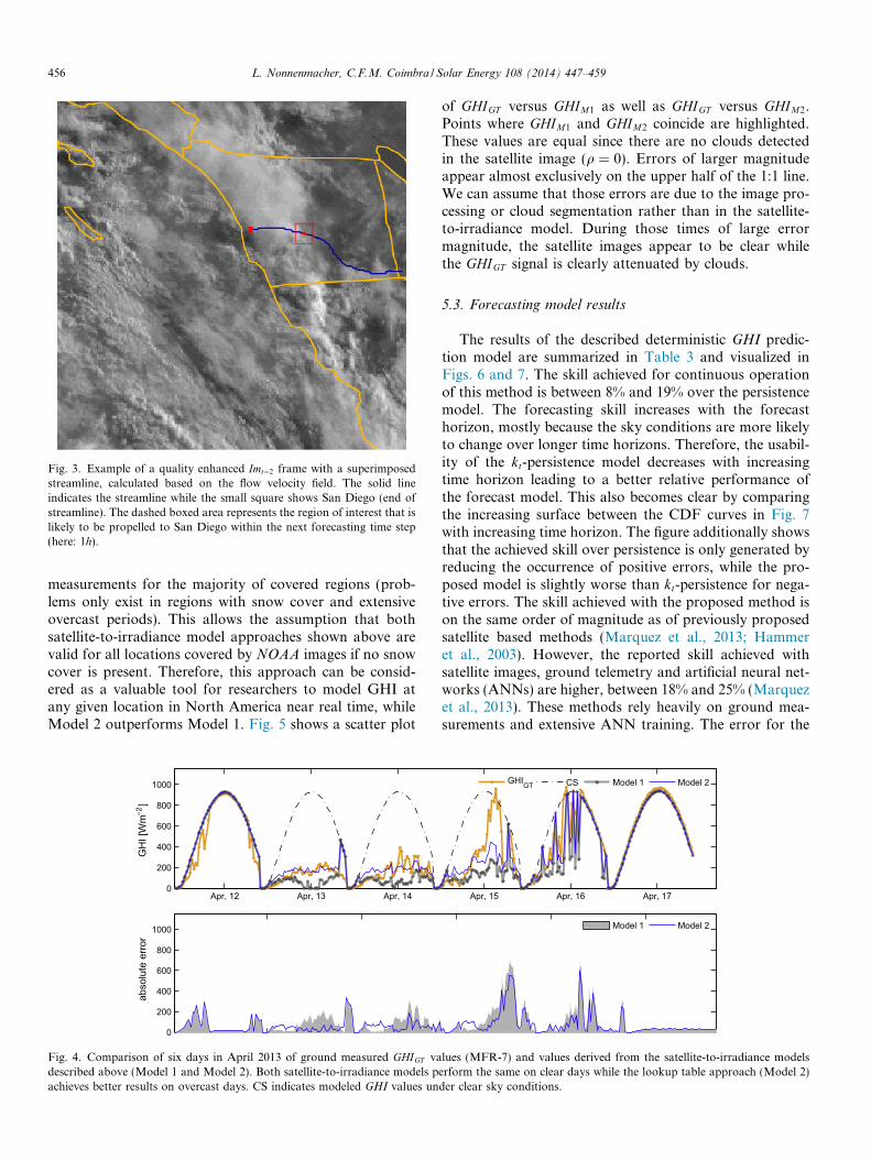
Fig. 3. Example of a quality enhanced Imt¼2 frame with a superimposedstreamline, calculated based on the flow velocity field. The solid lineindicates the streamline while the small square shows San Diego (end ofstreamline). The dashed boxed area represents the region of interest that islikely to be propelled to San Diego within the next forecasting time step(here: 1h).

456 L. Nonnenmacher, C.F.M. Coimbra / Solar Energy 108 (2014) 447–459

measurements for the majority of covered regions (prob-lems only exist in regions with snow cover and extensiveovercast periods). This allows the assumption that bothsatellite-to-irradiance model approaches shown above arevalid for all locations covered by NOAA images if no snowcover is present. Therefore, this approach can be consid-ered as a valuable tool for researchers to model GHI atany given location in North America near real time, whileModel 2 outperforms Model 1. Fig. 5 shows a scatter plot

Apr, 12 Apr, 13 Apr, 140

200

400

600

800

1000

GH

I [W

m−2

]

0

200

400

600

800

1000

abso

lute

err

or

Fig. 4. Comparison of six days in April 2013 of ground measured GHIGT vadescribed above (Model 1 and Model 2). Both satellite-to-irradiance models pachieves better results on overcast days. CS indicates modeled GHI values un

of GHIGT versus GHIM1 as well as GHIGT versus GHIM2.Points where GHIM1 and GHIM2 coincide are highlighted.These values are equal since there are no clouds detectedin the satellite image (q ¼ 0). Errors of larger magnitudeappear almost exclusively on the upper half of the 1:1 line.We can assume that those errors are due to the image pro-cessing or cloud segmentation rather than in the satellite-to-irradiance model. During those times of large errormagnitude, the satellite images appear to be clear whilethe GHIGT signal is clearly attenuated by clouds.

5.3. Forecasting model results

The results of the described deterministic GHI predic-tion model are summarized in Table 3 and visualized inFigs. 6 and 7. The skill achieved for continuous operationof this method is between 8% and 19% over the persistencemodel. The forecasting skill increases with the forecasthorizon, mostly because the sky conditions are more likelyto change over longer time horizons. Therefore, the usabil-ity of the kt-persistence model decreases with increasingtime horizon leading to a better relative performance ofthe forecast model. This also becomes clear by comparingthe increasing surface between the CDF curves in Fig. 7with increasing time horizon. The figure additionally showsthat the achieved skill over persistence is only generated byreducing the occurrence of positive errors, while the pro-posed model is slightly worse than kt-persistence for nega-tive errors. The skill achieved with the proposed method ison the same order of magnitude as of previously proposedsatellite based methods (Marquez et al., 2013; Hammeret al., 2003). However, the reported skill achieved withsatellite images, ground telemetry and artificial neural net-works (ANNs) are higher, between 18% and 25% (Marquezet al., 2013). These methods rely heavily on ground mea-surements and extensive ANN training. The error for the

Apr, 15 Apr, 16 Apr, 17

GHIGT CS Model 1 Model 2

Model 1 Model 2

lues (MFR-7) and values derived from the satellite-to-irradiance modelserform the same on clear days while the lookup table approach (Model 2)der clear sky conditions.

0 200 400 600 800 10000

100

200

300

400

500

600

700

800

900

1000

GH

I GT [W

m−2

]

Modeled GHI [Wm−2 ]

Model 2Model 1Model 1 = Model 2

Fig. 5. Scatter plot of GHIGT against the values obtained with GHIM1 andGHIM2. It can be seen that the error of Model 2 is generally smaller thanfrom Model 1. Model 1 tends to underestimate irradiance under overcastconditions. This is due to the fact that for Model 2 kt;min ¼ 0:16 whileModel 1 allows for kt;min ¼ 0 which cannot occur during daylight times.Yellow markers indicate that values from Model 1 equal values of Model2, obtained when q ¼ 0 in the satellite image. In these cases, the resultingerrors are large and due to undetected clouds in the satellite image. (Forinterpretation of the references to colour in this figure legend, the reader isreferred to the web version of this article.)

L. Nonnenmacher, C.F.M. Coimbra / Solar Energy 108 (2014) 447–459 457

1h-ahead (rMAE = 8.83% and 8.62%) forecast is of lowermagnitude than other solely deterministic models (e.g.Hammer et al., 1999 rMAE = 12–15%). A comparison ofour results to the results mentioned by Perez et al. (2010)suggests that our new method can be used in addition or

Oct, 13 Oct, 14 Oct,0

200

400

600

800

GH

I [W

m−2]

0

200

400

600

800

abso

lute

err

or

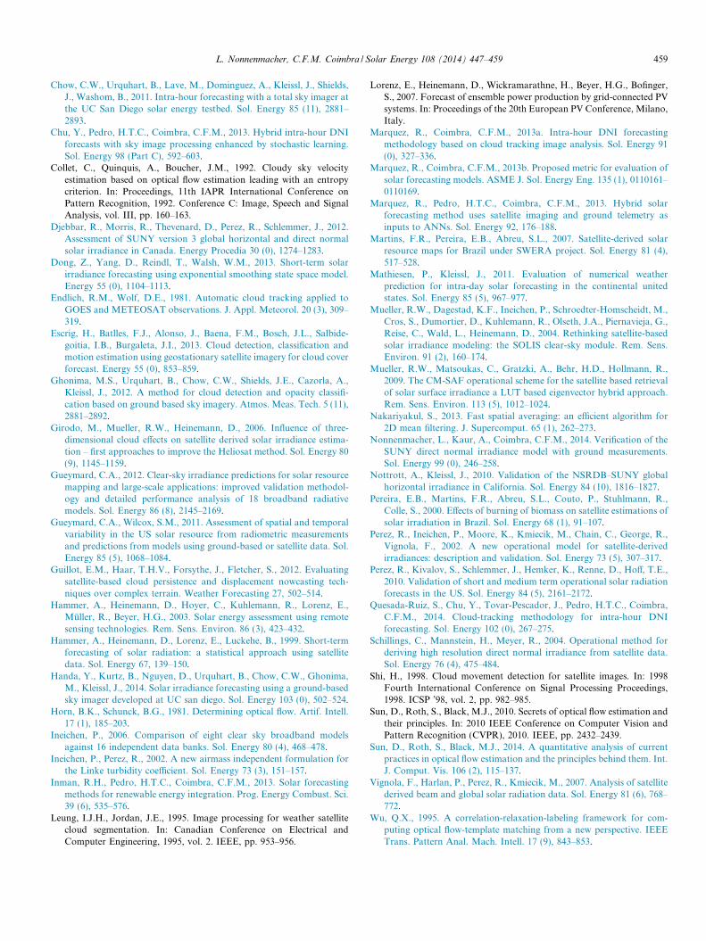
Fig. 6. Comparison of five example days in October 2013 of ground measuredresults from the kt-persistence model. The second part of the figure shows thebetween ground truth and the forecasted values compared to the error of kt-p

as an alternative and provide similar or better results,depending on the location specific irradiance characteris-tics. Additionally, the temporal resolution of this forecastwith an update every 15 min is higher than for the citedstudies (Hammer et al., 1999, 2003; Marquez et al.,2013). Fig. 6 provides an example of the results of the pro-posed forecasting model compared to ground truth valuesand the kt-persistence model. This sequence of consecutivedays has been chosen as an example because it covers var-ious sky conditions. In general, the forecasting methodreduces the error compared to kt-persistence. This charac-teristic is consistent with the positive forecasting skill forall forecast horizons (see Table 3). Since there are multiplelayers of data processing in this study, a closer look at thecritical sources of error helps to clarify the origin of overallerrors. The forecasting performance (and thus the skill) ofthe proposed method is limited by the accuracy of the satel-lite-to-irradiance model. Additional sources of error aredue to image processing, inaccurate cloud tracking andthe simplifications made with the frozen cloud assumption.An example of a typical error is shown in Fig. 6 where anon-captured ramp event in the GHIGT signal occurs mid-day on 16-October-2013. For this particular event, thecloud image appears to be clear while a significant GHIattenuation is measured on the ground. This type of erroris caused normally during to the image transfer and preli-minary processing of the satellite images.

6. Conclusions

A remote sensing-based GHI forecasting methodologywas proposed and successfully applied to predict 15 minaverages of GHI on the Earth surface for 1h-, 2h- and 3h

15 Oct, 16 Oct, 18

GHIGT kt−persistence Forecasting Model

Err. kt−pers. Err. Forec.

GHIGT values, results from the proposed 1h-ahead forecasting method anderror of both models. The proposed forecasting model reduces the error

ersistence.

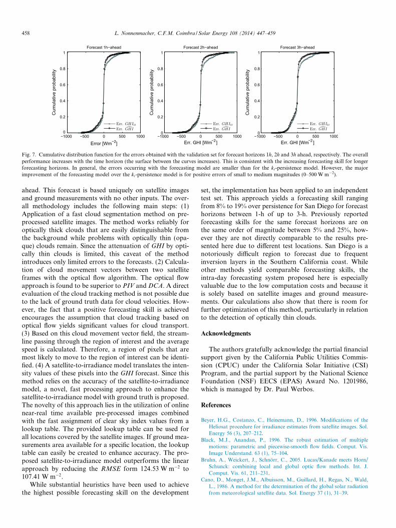
Fig. 7. Cumulative distribution function for the errors obtained with the validation set for forecast horizons 1h, 2h and 3h ahead, respectively. The overallperformance increases with the time horizon (the surface between the curves increases). This is consistent with the increasing forecasting skill for longerforecasting horizons. In general, the errors occurring with the forecasting model are smaller than for the kt-persistence model. However, the majorimprovement of the forecasting model over the kt-persistence model is for positive errors of small to medium magnitudes (0–500 W m�2).

458 L. Nonnenmacher, C.F.M. Coimbra / Solar Energy 108 (2014) 447–459

ahead. This forecast is based uniquely on satellite imagesand ground measurements with no other inputs. The over-all methodology includes the following main steps: (1)Application of a fast cloud segmentation method on pre-processed satellite images. The method works reliably foroptically thick clouds that are easily distinguishable fromthe background while problems with optically thin (opa-que) clouds remain. Since the attenuation of GHI by opti-cally thin clouds is limited, this caveat of the methodintroduces only limited errors to the forecasts. (2) Calcula-tion of cloud movement vectors between two satelliteframes with the optical flow algorithm. The optical flowapproach is found to be superior to PIV and DCA. A directevaluation of the cloud tracking method is not possible dueto the lack of ground truth data for cloud velocities. How-ever, the fact that a positive forecasting skill is achievedencourages the assumption that cloud tracking based onoptical flow yields significant values for cloud transport.(3) Based on this cloud movement vector field, the stream-line passing through the region of interest and the averagespeed is calculated. Therefore, a region of pixels that aremost likely to move to the region of interest can be identi-fied. (4) A satellite-to-irradiance model translates the inten-sity values of these pixels into the GHI forecast. Since thismethod relies on the accuracy of the satellite-to-irradiancemodel, a novel, fast processing approach to enhance thesatellite-to-irradiance model with ground truth is proposed.The novelty of this approach lies in the utilization of onlinenear-real time available pre-processed images combinedwith the fast assignment of clear sky index values from alookup table. The provided lookup table can be used forall locations covered by the satellite images. If ground mea-surements area available for a specific location, the lookuptable can easily be created to enhance accuracy. The pro-posed satellite-to-irradiance model outperforms the linearapproach by reducing the RMSE form 124:53 W m�2 to107:41 W m�2.

While substantial heuristics have been used to achievethe highest possible forecasting skill on the development

set, the implementation has been applied to an independenttest set. This approach yields a forecasting skill rangingfrom 8% to 19% over persistence for San Diego for forecasthorizons between 1-h of up to 3-h. Previously reportedforecasting skills for the same forecast horizons are onthe same order of magnitude between 5% and 25%, how-ever they are not directly comparable to the results pre-sented here due to different test locations. San Diego is anotoriously difficult region to forecast due to frequentinversion layers in the Southern California coast. Whileother methods yield comparable forecasting skills, theintra-day forecasting system proposed here is especiallyvaluable due to the low computation costs and because itis solely based on satellite images and ground measure-ments. Our calculations also show that there is room forfurther optimization of this method, particularly in relationto the detection of optically thin clouds.

Acknowledgments

The authors gratefully acknowledge the partial financialsupport given by the California Public Utilities Commis-sion (CPUC) under the California Solar Initiative (CSI)Program, and the partial support by the National ScienceFoundation (NSF) EECS (EPAS) Award No. 1201986,which is managed by Dr. Paul Werbos.

References

Beyer, H.G., Costanzo, C., Heinemann, D., 1996. Modifications of theHeliosat procedure for irradiance estimates from satellite images. Sol.Energy 56 (3), 207–212.

Black, M.J., Anandan, P., 1996. The robust estimation of multiplemotions: parametric and piecewise-smooth flow fields. Comput. Vis.Image Understand. 63 (1), 75–104.

Bruhn, A., Weickert, J., Schnorr, C., 2005. Lucas/Kanade meets Horn/Schunck: combining local and global optic flow methods. Int. J.Comput. Vis. 61, 211–231.

Cano, D., Monget, J.M., Albuisson, M., Guillard, H., Regas, N., Wald,L., 1986. A method for the determination of the global solar radiationfrom meteorological satellite data. Sol. Energy 37 (1), 31–39.

L. Nonnenmacher, C.F.M. Coimbra / Solar Energy 108 (2014) 447–459 459

Chow, C.W., Urquhart, B., Lave, M., Dominguez, A., Kleissl, J., Shields,J., Washom, B., 2011. Intra-hour forecasting with a total sky imager atthe UC San Diego solar energy testbed. Sol. Energy 85 (11), 2881–2893.

Chu, Y., Pedro, H.T.C., Coimbra, C.F.M., 2013. Hybrid intra-hour DNIforecasts with sky image processing enhanced by stochastic learning.Sol. Energy 98 (Part C), 592–603.

Collet, C., Quinquis, A., Boucher, J.M., 1992. Cloudy sky velocityestimation based on optical flow estimation leading with an entropycriterion. In: Proceedings, 11th IAPR International Conference onPattern Recognition, 1992. Conference C: Image, Speech and SignalAnalysis, vol. III, pp. 160–163.

Djebbar, R., Morris, R., Thevenard, D., Perez, R., Schlemmer, J., 2012.Assessment of SUNY version 3 global horizontal and direct normalsolar irradiance in Canada. Energy Procedia 30 (0), 1274–1283.

Dong, Z., Yang, D., Reindl, T., Walsh, W.M., 2013. Short-term solarirradiance forecasting using exponential smoothing state space model.Energy 55 (0), 1104–1113.

Endlich, R.M., Wolf, D.E., 1981. Automatic cloud tracking applied toGOES and METEOSAT observations. J. Appl. Meteorol. 20 (3), 309–319.

Escrig, H., Batlles, F.J., Alonso, J., Baena, F.M., Bosch, J.L., Salbide-goitia, I.B., Burgaleta, J.I., 2013. Cloud detection, classification andmotion estimation using geostationary satellite imagery for cloud coverforecast. Energy 55 (0), 853–859.

Ghonima, M.S., Urquhart, B., Chow, C.W., Shields, J.E., Cazorla, A.,Kleissl, J., 2012. A method for cloud detection and opacity classifi-cation based on ground based sky imagery. Atmos. Meas. Tech. 5 (11),2881–2892.

Girodo, M., Mueller, R.W., Heinemann, D., 2006. Influence of three-dimensional cloud effects on satellite derived solar irradiance estima-tion – first approaches to improve the Heliosat method. Sol. Energy 80(9), 1145–1159.

Gueymard, C.A., 2012. Clear-sky irradiance predictions for solar resourcemapping and large-scale applications: improved validation methodol-ogy and detailed performance analysis of 18 broadband radiativemodels. Sol. Energy 86 (8), 2145–2169.

Gueymard, C.A., Wilcox, S.M., 2011. Assessment of spatial and temporalvariability in the US solar resource from radiometric measurementsand predictions from models using ground-based or satellite data. Sol.Energy 85 (5), 1068–1084.

Guillot, E.M., Haar, T.H.V., Forsythe, J., Fletcher, S., 2012. Evaluatingsatellite-based cloud persistence and displacement nowcasting tech-niques over complex terrain. Weather Forecasting 27, 502–514.

Hammer, A., Heinemann, D., Hoyer, C., Kuhlemann, R., Lorenz, E.,Muller, R., Beyer, H.G., 2003. Solar energy assessment using remotesensing technologies. Rem. Sens. Environ. 86 (3), 423–432.

Hammer, A., Heinemann, D., Lorenz, E., Luckehe, B., 1999. Short-termforecasting of solar radiation: a statistical approach using satellitedata. Sol. Energy 67, 139–150.

Handa, Y., Kurtz, B., Nguyen, D., Urquhart, B., Chow, C.W., Ghonima,M., Kleissl, J., 2014. Solar irradiance forecasting using a ground-basedsky imager developed at UC san diego. Sol. Energy 103 (0), 502–524.

Horn, B.K., Schunck, B.G., 1981. Determining optical flow. Artif. Intell.17 (1), 185–203.

Ineichen, P., 2006. Comparison of eight clear sky broadband modelsagainst 16 independent data banks. Sol. Energy 80 (4), 468–478.

Ineichen, P., Perez, R., 2002. A new airmass independent formulation forthe Linke turbidity coefficient. Sol. Energy 73 (3), 151–157.

Inman, R.H., Pedro, H.T.C., Coimbra, C.F.M., 2013. Solar forecastingmethods for renewable energy integration. Prog. Energy Combust. Sci.39 (6), 535–576.

Leung, I.J.H., Jordan, J.E., 1995. Image processing for weather satellitecloud segmentation. In: Canadian Conference on Electrical andComputer Engineering, 1995, vol. 2. IEEE, pp. 953–956.

Lorenz, E., Heinemann, D., Wickramarathne, H., Beyer, H.G., Bofinger,S., 2007. Forecast of ensemble power production by grid-connected PVsystems. In: Proceedings of the 20th European PV Conference, Milano,Italy.

Marquez, R., Coimbra, C.F.M., 2013a. Intra-hour DNI forecastingmethodology based on cloud tracking image analysis. Sol. Energy 91(0), 327–336.

Marquez, R., Coimbra, C.F.M., 2013b. Proposed metric for evaluation ofsolar forecasting models. ASME J. Sol. Energy Eng. 135 (1), 0110161–0110169.

Marquez, R., Pedro, H.T.C., Coimbra, C.F.M., 2013. Hybrid solarforecasting method uses satellite imaging and ground telemetry asinputs to ANNs. Sol. Energy 92, 176–188.

Martins, F.R., Pereira, E.B., Abreu, S.L., 2007. Satellite-derived solarresource maps for Brazil under SWERA project. Sol. Energy 81 (4),517–528.

Mathiesen, P., Kleissl, J., 2011. Evaluation of numerical weatherprediction for intra-day solar forecasting in the continental unitedstates. Sol. Energy 85 (5), 967–977.

Mueller, R.W., Dagestad, K.F., Ineichen, P., Schroedter-Homscheidt, M.,Cros, S., Dumortier, D., Kuhlemann, R., Olseth, J.A., Piernavieja, G.,Reise, C., Wald, L., Heinemann, D., 2004. Rethinking satellite-basedsolar irradiance modeling: the SOLIS clear-sky module. Rem. Sens.Environ. 91 (2), 160–174.

Mueller, R.W., Matsoukas, C., Gratzki, A., Behr, H.D., Hollmann, R.,2009. The CM-SAF operational scheme for the satellite based retrievalof solar surface irradiance a LUT based eigenvector hybrid approach.Rem. Sens. Environ. 113 (5), 1012–1024.

Nakariyakul, S., 2013. Fast spatial averaging: an efficient algorithm for2D mean filtering. J. Supercomput. 65 (1), 262–273.

Nonnenmacher, L., Kaur, A., Coimbra, C.F.M., 2014. Verification of theSUNY direct normal irradiance model with ground measurements.Sol. Energy 99 (0), 246–258.

Nottrott, A., Kleissl, J., 2010. Validation of the NSRDB–SUNY globalhorizontal irradiance in California. Sol. Energy 84 (10), 1816–1827.

Pereira, E.B., Martins, F.R., Abreu, S.L., Couto, P., Stuhlmann, R.,Colle, S., 2000. Effects of burning of biomass on satellite estimations ofsolar irradiation in Brazil. Sol. Energy 68 (1), 91–107.

Perez, R., Ineichen, P., Moore, K., Kmiecik, M., Chain, C., George, R.,Vignola, F., 2002. A new operational model for satellite-derivedirradiances: description and validation. Sol. Energy 73 (5), 307–317.

Perez, R., Kivalov, S., Schlemmer, J., Hemker, K., Renne, D., Hoff, T.E.,2010. Validation of short and medium term operational solar radiationforecasts in the US. Sol. Energy 84 (5), 2161–2172.

Quesada-Ruiz, S., Chu, Y., Tovar-Pescador, J., Pedro, H.T.C., Coimbra,C.F.M., 2014. Cloud-tracking methodology for intra-hour DNIforecasting. Sol. Energy 102 (0), 267–275.

Schillings, C., Mannstein, H., Meyer, R., 2004. Operational method forderiving high resolution direct normal irradiance from satellite data.Sol. Energy 76 (4), 475–484.

Shi, H., 1998. Cloud movement detection for satellite images. In: 1998Fourth International Conference on Signal Processing Proceedings,1998. ICSP ’98, vol. 2, pp. 982–985.

Sun, D., Roth, S., Black, M.J., 2010. Secrets of optical flow estimation andtheir principles. In: 2010 IEEE Conference on Computer Vision andPattern Recognition (CVPR), 2010. IEEE, pp. 2432–2439.

Sun, D., Roth, S., Black, M.J., 2014. A quantitative analysis of currentpractices in optical flow estimation and the principles behind them. Int.J. Comput. Vis. 106 (2), 115–137.

Vignola, F., Harlan, P., Perez, R., Kmiecik, M., 2007. Analysis of satellitederived beam and global solar radiation data. Sol. Energy 81 (6), 768–772.

Wu, Q.X., 1995. A correlation-relaxation-labeling framework for com-puting optical flow-template matching from a new perspective. IEEETrans. Pattern Anal. Mach. Intell. 17 (9), 843–853.