stock market volatility: identifying major drivers and the...
TRANSCRIPT

Center for Quantitative Risk Analysis (CEQURA)Department of Statistics, University of Munich (LMU)
Max Planck Society (MPG)
Stock Market Volatility:Identifying Major Drivers and the Nature of Their
Impact
Stefan Mittnik (CEQURA, LMU)Nikolay Robinzonov (CEQURA)
Martin Spindler (CEQURA, MPG, visiting MIT)
Annual Meeting of the Austrian Statistical Society
September 10, 2014, Innsbruck

Outline
1 Introduction and Motivation
2 Econometric Model
3 Estimation
4 Illustration
5 Data Set
6 Empirical Results
Predictive Performance
Where does the improvement come from?
Driving Factors
1 / 27

Introduction and Motivation
Why volatility?
“Time-varying volatility is endemic in financial markets.”
Shephard and Andersen (2009, p. 233)
2 / 27
Introduction and Motivation
Motivation
• Importance of understanding, modeling and forecasting volatility:+ We quantify risk.
• Applications:+ Option valuation (dynamic volatility)+ Risk management (VaR, ES)+ Portfolio optimization and asset allocation
3 / 27
Introduction and Motivation Research Question
Research Question
Explain: Insights into the “anatomy” of volatility:
1 Identify small groups of influential drivers from manypotential factors for the stock market.
2 Identify volatility regimes of these drivers.3 Quantify regime dependence.4 Econometric challenge: large set of potential factors (model
selection)
Forecast: Can we use these factors to forecast volatility?
4 / 27
Introduction and Motivation Research Question
Linear model
x
y
−4
−2
0
2
4
6
0 1 2 3
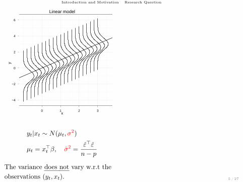
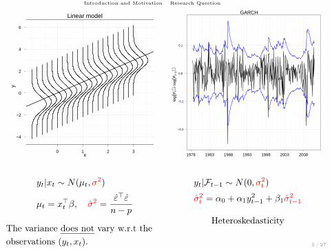
yt|xt ∼ N(µt, σ2)
µt = x>t β, σ2 =ε>ε
n− p
The variance does not vary w.r.t theobservations (yt, xt).
GARCH
log(
Pt)−
log(
Pt−
1)
−0.2
−0.1
0.0
0.1
1978 1983 1988 1993 1998 2003 2008
yt|Ft−1 ∼ N(0, σ2t )
σ2t = α0 + α1y
2t−1 + β1σ
2t−1
Heteroskedasticity
5 / 27
Introduction and Motivation Research Question
Linear model
x
y
−4
−2
0
2
4
6
0 1 2 3
yt|xt ∼ N(µt, σ2)
µt = x>t β, σ2 =ε>ε
n− p
The variance does not vary w.r.t theobservations (yt, xt).
GARCH
log(
Pt)−
log(
Pt−
1)
−0.2
−0.1
0.0
0.1
1978 1983 1988 1993 1998 2003 2008
yt|Ft−1 ∼ N(0, σ2t )
σ2t = α0 + α1y
2t−1 + β1σ
2t−1
Heteroskedasticity
5 / 27
Econometric Model
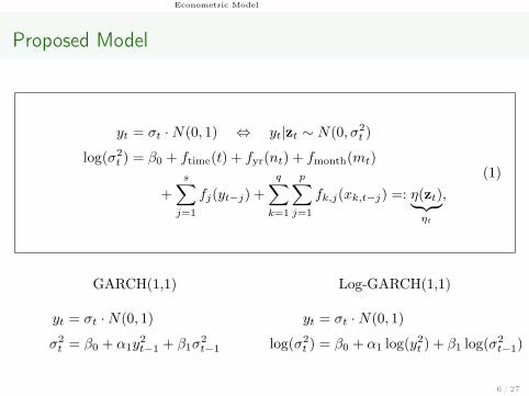
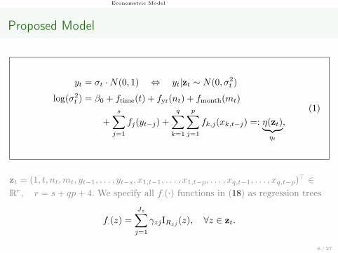
Proposed Model
yt = σt ·N(0, 1) ⇔ yt|zt ∼ N(0, σ2t )
log(σ2t ) = β0 + ftime(t) + fyr(nt) + fmonth(mt)
+
s∑j=1
fj(yt−j) +
q∑k=1
p∑j=1
fk,j(xk,t−j) =: η(zt)︸ ︷︷ ︸ηt
,
(1)
GARCH(1,1)
yt = σt ·N(0, 1)
σ2t = β0 + α1y
2t−1 + β1σ
2t−1
Log-GARCH(1,1)
yt = σt ·N(0, 1)
log(σ2t ) = β0 + α1 log(y2t ) + β1 log(σ2
t−1)
6 / 27
Econometric Model
Proposed Model
yt = σt ·N(0, 1) ⇔ yt|zt ∼ N(0, σ2t )
log(σ2t ) = β0 + ftime(t) + fyr(nt) + fmonth(mt)
+
s∑j=1
fj(yt−j) +
q∑k=1
p∑j=1
fk,j(xk,t−j) =: η(zt)︸ ︷︷ ︸ηt
,
(1)
zt = (1, t, nt,mt, yt−1, . . . , yt−s, x1,t−1, . . . , x1,t−p, . . . , xq,t−1, . . . , xq,t−p)> ∈
Rr, r = s+ qp+ 4. We specify all f·(·) functions in (18) as regression trees
f.(z) =
Jz∑j=1
γzjIRzj (z), ∀z ∈ zt.
6 / 27

Estimation

Estimation
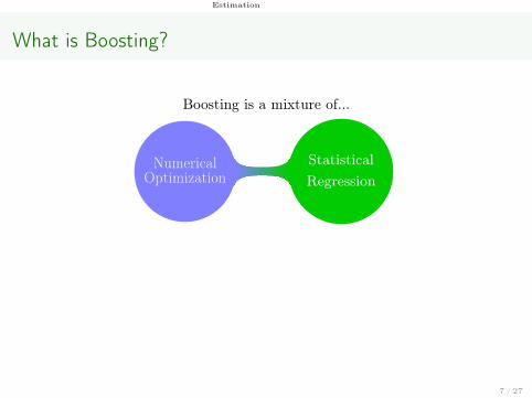
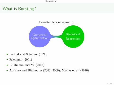
What is Boosting?
Boosting is a mixture of...
NumericalOptimization
StatisticalRegression
• Freund and Schapire (1996)
• Friedman (2001)
• Bühlmann and Yu (2003)
• Audrino and Bühlmann (2003, 2009), Matías et al. (2010)
7 / 27
Estimation
What is Boosting?
Boosting is a mixture of...
NumericalOptimization
StatisticalRegression
• Freund and Schapire (1996)
• Friedman (2001)
• Bühlmann and Yu (2003)
• Audrino and Bühlmann (2003, 2009), Matías et al. (2010)
7 / 27
Estimation
What is Boosting?
Boosting is a mixture of...
NumericalOptimization
StatisticalRegression
• Freund and Schapire (1996)
• Friedman (2001)
• Bühlmann and Yu (2003)
• Audrino and Bühlmann (2003, 2009), Matías et al. (2010)
7 / 27

Estimation
Estimation Problem
V (yt|zt) = σ2t =: eηt
• Objective: Obtain an estimate η∗
η∗ = arg minη
E [L(y, η)] (2)
⇒ Loss function: Lt =1
2
[lnσ2
t +y2tσ2t
]σ2t=e
ηt
=1
2
[ηt +
y2teηt
]
8 / 27

Estimation
Estimation Problem
V (yt|zt) = σ2t =: eηt
• Objective: Obtain an estimate η∗:
η∗ = arg minη
E [L(y, η)] (2)
• In practice, we minimize the empirical risk:
η∗ = η(z; β) = arg minη
1
T
T∑t=1
L(yt, η(zt;β)). (3)
9 / 27
Estimation
Steepest Descent
Y1
Y2
−2
−1
0
1
2
−2 −1 0 1 2
value
2
4
6
8
10
12
14
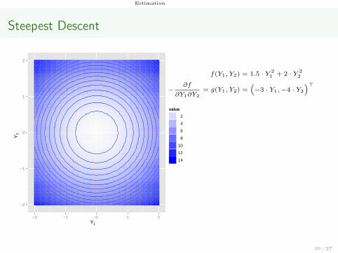
f(Y1, Y2) = 1.5 · Y 21 + 2 · Y 2
2
−∂f
∂Y1∂Y2
= g(Y1, Y2) =(−3 · Y1,−4 · Y2
)>
Y[0]
= (−1.5, 2)>
g(Y[0]
) = (4.5,−8)>
Y[1]
= Y[0]
+ 1/10︸︷︷︸ν
· g(Y [0])︸ ︷︷ ︸
update
= (−1.05, 1.2)>
...
Y[k]
= Y[k−1]
+ 1/10 · g(Y [k−1])
...
10 / 27
Estimation
Steepest Descent
Y1
Y2
−2
−1
0
1
2 ●
●
●
●
●
●
●
●
−2 −1 0 1 2
value
● 2
● 4
● 6
● 8
● 10
● 12
● 14
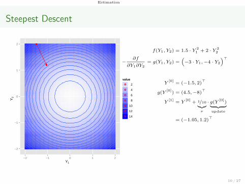
f(Y1, Y2) = 1.5 · Y 21 + 2 · Y 2
2
−∂f
∂Y1∂Y2
= g(Y1, Y2) =(−3 · Y1,−4 · Y2
)>
Y[0]
= (−1.5, 2)>
g(Y[0]
) = (4.5,−8)>
Y[1]
= Y[0]
+ 1/10︸︷︷︸ν
· g(Y [0])︸ ︷︷ ︸
update
= (−1.05, 1.2)>
...
Y[k]
= Y[k−1]
+ 1/10 · g(Y [k−1])
...
10 / 27
Estimation
Steepest Descent
Y1
Y2
−2
−1
0
1
2 ●
●
●
●
●
●
●
●
●
●
●
●
●
●●
●
−2 −1 0 1 2
value
●● 2
●● 4
●● 6
●● 8
●● 10
●● 12
●● 14
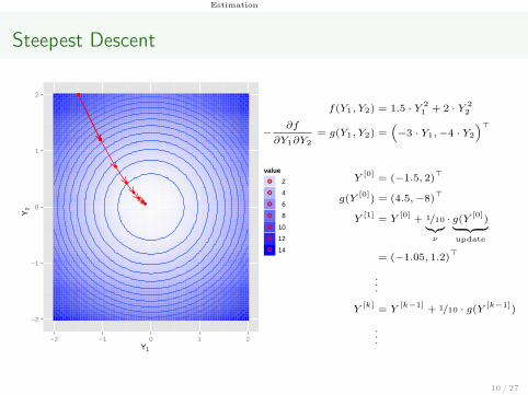
f(Y1, Y2) = 1.5 · Y 21 + 2 · Y 2
2
−∂f
∂Y1∂Y2
= g(Y1, Y2) =(−3 · Y1,−4 · Y2
)>
Y[0]
= (−1.5, 2)>
g(Y[0]
) = (4.5,−8)>
Y[1]
= Y[0]
+ 1/10︸︷︷︸ν
· g(Y [0])︸ ︷︷ ︸
update
= (−1.05, 1.2)>
...
Y[k]
= Y[k−1]
+ 1/10 · g(Y [k−1])
...
10 / 27

Estimation
Estimation Problem
η∗= η(z; β) = arg min
η
1
T
T∑t=1
L(yt, η(zt;β)) (3)
1 Given any approximation η[m−1]t = η(zt; β
[m−1]) the current negative gradient is
g[m]t := −
[∂
∂ηL(yt, η)
]η=η
[m−1]t
, t = 1, . . . , T
which gives the steepest-descent direction.
2 Then, we estimate the gradient:
• Estimate the negative gradient by each predictor separately
γ[m]j = arg min
γj
[fj(zj ;γj)→ g
[m]j
], j = 1 . . . , r
• sm = arg minj∈{1,...,r}
∑Tt=1
(g[m]t − fj(zjt; γ[m]
j ))2
3 Updateη(zt; β
[m]) = η(zt; β
[m−1]) + ν ·
���@@@
g[m]︸︷︷︸
steepestdescent
, t = 1, . . . , T.
11 / 27
Estimation
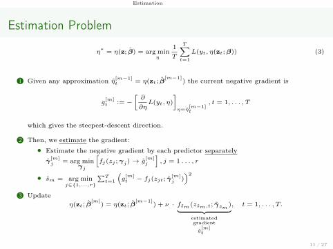
Estimation Problem
η∗= η(z; β) = arg min
η
1
T
T∑t=1
L(yt, η(zt;β)) (3)
1 Given any approximation η[m−1]t = η(zt; β
[m−1]) the current negative gradient is
g[m]t := −
[∂
∂ηL(yt, η)
]η=η
[m−1]t
, t = 1, . . . , T
which gives the steepest-descent direction.
2 Then, we estimate the gradient:
• Estimate the negative gradient by each predictor separately
γ[m]j = arg min
γj
[fj(zj ;γj)→ g
[m]j
], j = 1 . . . , r
• sm = arg minj∈{1,...,r}
∑Tt=1
(g[m]t − fj(zjt; γ[m]
j ))2
3 Updateη(zt; β
[m]) = η(zt; β
[m−1]) + ν · fsm (zsm,t; γsm )︸ ︷︷ ︸
estimatedgradient
g[m]t
, t = 1, . . . , T.
11 / 27

Illustration

Illustration
Simulation
Simulation:
yt = exp(ηt/2)εt
ηt = 0.1 + 2x1,t + 2I[0.1,0.5](x2,t)x2,t − 0.6I[−0.5,−0.2](x3,t)+
0x4,t + 0x5,t + 0x6,t,
with εtiid∼ N(0, 1) and xi,t being the t-th observation of Xi ∼ U [−0.5, 0.5],
i = 1, . . . , 6, t = 1, . . . , T , T = 400. The model:
ηt = β0 + β1x1,t +
J2∑j=1
γ2jIR2j (x2,t) +
J3∑j=1
γ3jIR3j (x3,t)+
β4x4,t + β5x5,t + β6x6,t,
where R2j and R3j represent the estimated partitions of the domains of X2
and X3.12 / 27
Illustration
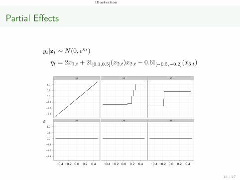
Partial Effects
yt|zt ∼ N(0, eηt)
ηt = 2x1,t + 2I[0.1,0.5](x2,t)x2,t − 0.6I[−0.5,−0.2](x3,t)
η t
−1.5
−1.0
−0.5
0.0
0.5
1.0
−1.5
−1.0
−0.5
0.0
0.5
1.0
X1
X4
−0.4 −0.2 0.0 0.2 0.4
X2
X5
−0.4 −0.2 0.0 0.2 0.4
X3
X6
−0.4 −0.2 0.0 0.2 0.4
13 / 27
Illustration
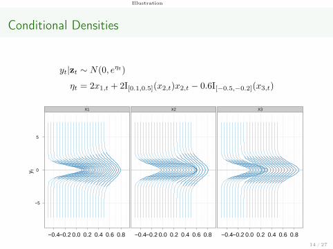
Conditional Densities
yt|zt ∼ N(0, eηt)
ηt = 2x1,t + 2I[0.1,0.5](x2,t)x2,t − 0.6I[−0.5,−0.2](x3,t)
y t
−5
0
5
X1
−0.4−0.2 0.0 0.2 0.4 0.6 0.8
X2
−0.4−0.2 0.0 0.2 0.4 0.6 0.8
X3
−0.4−0.2 0.0 0.2 0.4 0.6 0.8
14 / 27

Data Set
Data Set
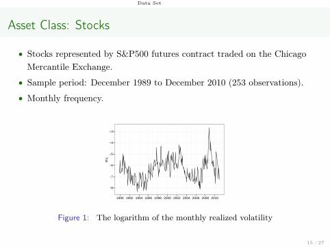
Asset Class: Stocks
• Stocks represented by S&P500 futures contract traded on the ChicagoMercantile Exchange.
• Sample period: December 1989 to December 2010 (253 observations).
• Monthly frequency.
−8
−7
−6
−5
−4
−3
1990 1992 1994 1996 1998 2000 2002 2004 2006 2008 2010
RV
t
Figure 1: The logarithm of the monthly realized volatility
15 / 27

Data Set
Macroeconomics and Financial Factors
Large set of macroeconomic and financial factors
• Equity Market Variables and Risk Factors
• Interest Rates, Spreads and Bond Market Factors
• FX Variables
• Liquidity and Risk Variables
• Macroeconomic Variables
16 / 27
Data Set
Forecasting Strategy
• Sample period: December 1989 to December 2010 (253 months)
• Estimation: 38 regressors with first and second lag (q = 38, p = 2) andfirst and second lag of realized volatility (s = 2) and changes of realizedvolatilityIn total: r = 84 predictors
• Rolling window scheme (window size: 153 months)
• Evaluation period: June 2002 to September 2010 (100 months)
• Direct forecasting approach; multi-period forecasts for one to six months
• Forecast evaluation by mean squared error. We will compare ex-post(realized volatility) estimations σ2
RV with ex-ante predictions exp(ηt).
17 / 27
Data Set
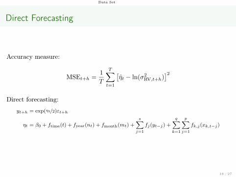
Direct Forecasting
Accuracy measure:
MSEt+h =1
T
T∑t=1
[ηt − ln(σ2
RV,t+h)]2
Direct forecasting:
yt+h = exp(ηt/2)εt+h
ηt = β0 + ftime(t) + fyear(nt) + fmonth(mt) +s∑j=1
fj(yt−j) +
q∑k=1
p∑j=1
fk,j(xk,t−j)
18 / 27

Empirical Results
Empirical Results Predictive Performance
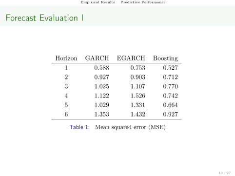
Forecast Evaluation I
Horizon GARCH EGARCH Boosting1 0.588 0.753 0.5272 0.927 0.903 0.7123 1.025 1.107 0.7704 1.122 1.526 0.7425 1.029 1.331 0.6646 1.353 1.432 0.927
Table 1: Mean squared error (MSE)
19 / 27
Empirical Results Predictive Performance
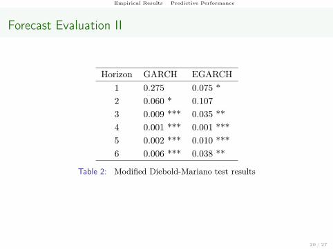
Forecast Evaluation II
Horizon GARCH EGARCH1 0.275 0.075 *2 0.060 * 0.1073 0.009 *** 0.035 **4 0.001 *** 0.001 ***5 0.002 *** 0.010 ***6 0.006 *** 0.038 **
Table 2: Modified Diebold-Mariano test results
20 / 27

Empirical Results Driving Factors
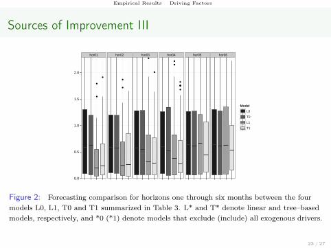
Sources of Improvement I
Forecasting accuracy is largely attributable to both the explanatory power ofthe drivers allowing drivers to affect volatility in a nonlinear fashion.
To disentangle these two sources of improvement, we adjust the model and uselinear instead of piecewise constant base learners by specifying
yt = exp(ηt/2)εt
ηt = β0 +
s∑j=1
βjyt−j +
q∑k=1
p∑j=1
γk,jxk,t−j =: η(zt),(4)
where the deterministic (seasonal) components are omitted.
21 / 27
Empirical Results Driving Factors
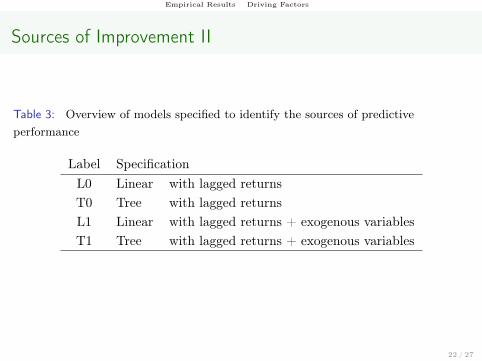
Sources of Improvement II
Table 3: Overview of models specified to identify the sources of predictiveperformance
Label SpecificationL0 Linear with lagged returnsT0 Tree with lagged returnsL1 Linear with lagged returns + exogenous variablesT1 Tree with lagged returns + exogenous variables
22 / 27
Empirical Results Driving Factors
Sources of Improvement III
hor01 hor02 hor03 hor04 hor05 hor06
●
●
●
●
●
●
●●
●
●
●
●
●
●●
●
●
●
●
●
●
●
0.0
0.5
1.0
1.5
2.0
Model
L0
T0
L1
T1
Figure 2: Forecasting comparison for horizons one through six months between the fourmodels L0, L1, T0 and T1 summarized in Table 3. L* and T* denote linear and tree–basedmodels, respectively, and *0 (*1) denote models that exclude (include) all exogenous drivers.
23 / 27
Empirical Results Driving Factors
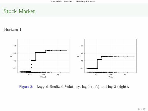
Stock Market
Horizon 1
●
●●
●●
●
●●●●●
●
●●
●
●
●
●
● ●●● ●
●
●
● ● ●●●
●
●
●
●
●
● ●
●
● ●
●
●
●
●
●
●
●
●
● ●●
●
●
●
●
●
●●
●
●●
●●●●
●
●
●●
● ●
●●
● ●
●
●
●
●
●
●
●
●
●●● ●●●
●● ●●
●
●●
●●●●
●
●
●
●
●●
●●●
●
● ● ●● ● ●●●●
●
●
●●●●● ●● ●●●
●
●
●
●
●
● ● ●
●●
●● ● ●●
●
●●● ● ●● ●
●●
●
●
●
●
●
●
●●●
●
●●
● ●●●● ●●
●
● ●●
● ●
●●
●●
● ●
●● ●●●●●●
●●
● ● ●
●●
●● ● ●●●●
●
●
●● ●●● ●●●
●
●● ●●●
●
● ●
●
● ●●
●●
●
●
●● ●● ●●
●●●
●
●●
●●●●
●●
●● ●
●
●
●
●● ●● ●
●
●●● ●●
●
● ● ●●●●
● ●●
● ●● ●● ●
●●
●●
●
● ●
●●
●● ●● ●●
●
● ●●
● ●●●●
●
●
●●● ●●
●
●
●
●
●●
●
●
●●●●
−0.2
0.0
0.2
0.4
−7 −5 −3RV.L1
η t ●●●
●
●●
●
●
●
●●●
●
●●
●
●
●
●
●
●
●●
●
●
●
● ●
●
●●
●●● ●
●
● ●
●
●
● ●
●
●● ●
●
●
●
● ●●
●
●
● ● ●●● ●●
●
●●●●●
● ●●
● ●
●●
●
● ●
●
●
●
●
● ●
●
●●● ●
●
●
●● ●●
●
●●●●●
●●
●
●
●
●●
●●●
●
● ●
●
● ● ●●●●
●●
●●●●● ●● ●●●
●● ●
●
●
● ● ●
●●
●● ● ●●
●
●●● ● ●● ●
●●
●
●●
●
●
●●
●●
●
●●
● ●●●● ●● ●● ●●
● ●
●●
●● ● ●●● ●●●●●●●
●
● ● ●
●●
●● ● ●●●●
●
● ●● ●●● ●●●
●
●● ●●●● ● ●● ● ●● ●●● ●●● ●● ●●●●●
● ●●
●●●●
●
●●
●
● ●
●
●
●● ●● ●
●
●●● ●●
●
● ● ●●●●
●
●
●
● ●● ●● ●
●
●
●●
● ● ●
●●
●● ●● ●●
●
● ●● ● ●●●●● ●●●● ●●● ●●
●
●●
●
● ●●●
−0.2
0.0
0.2
0.4
−7 −5 −3RV.L2
η t
Figure 3: Lagged Realized Volatility, lag 1 (left) and lag 2 (right).
24 / 27
Empirical Results Driving Factors
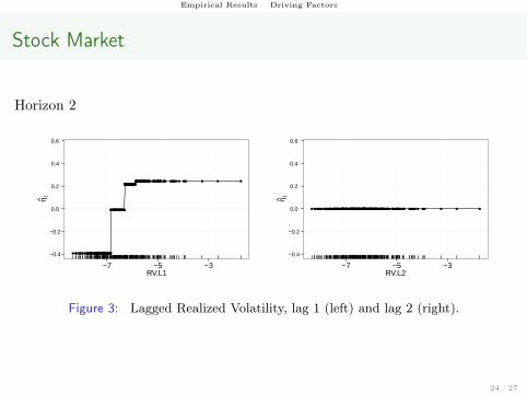
Stock Market
Horizon 2
●●
●
●●
●
●
●
●●●
●
●●
●
●
●
●
●
●
●●
●
●
●
● ●
●
●●
●●● ●
●
● ●
●
●
●●
●
●● ●
●
●
●
●●●
●
●
●● ●●● ●
●
●
●●●●
●
● ●●
● ●
●●
●
● ●
●
●
●
●
● ●
●
●●● ●
●
●
●●
●●
●
●●●●●
●●
●
●
●
●●
●●●
●
● ●
●
● ● ●●●●
●●
●●●●● ●● ●●●
●● ●
●
●
● ● ●
●●
●● ● ●●
●
●●● ● ●● ●
●●
●
●●
●
●
●●
●●
●
●●
● ●●●●
●● ●●
●●
● ●
●●
●●
● ●●●
●●●●●●●
●
●● ●
●●
●●
● ●●●●
●
●●● ●●● ●●
●
●
●●
●●●● ●
●● ●
●● ●●● ●●● ●●
●●●●●
● ●●
●●●●
●
●●
●
● ●
●
●
●● ●● ●
●
●●● ●●
●
● ● ●●●●
●
●
●
● ●● ●● ●
●
●
●●
● ●●
●●
●●
●●
●●
●
● ●● ● ●●●●● ●●●● ●●●
●●
●
●●
●
●●●●
−0.4
−0.2
0.0
0.2
0.4
0.6
−7 −5 −3RV.L1
η t
●●●● ●●●●●●●● ●●●● ●● ●● ●●● ●● ●● ● ●●● ●●● ● ●● ● ●● ● ●● ●● ●● ●● ● ●●●● ● ● ●●● ●●● ●●●●●● ●●● ● ●●● ● ●● ●● ●● ● ●●●● ●●● ●● ●●● ●●●●●●● ●● ● ●●●●● ●● ● ●● ● ●●●● ●●●●●●● ●● ●●● ●● ●● ●● ● ● ●●●● ● ●● ●●●● ● ●● ● ●● ●●●● ●●●●● ●●● ● ●●●● ●● ●● ●●● ● ●● ●● ● ●●● ●●●●●●●● ● ● ●●● ●● ● ●●●●● ● ●● ●●● ●●●● ●● ●●●● ● ●● ● ●● ●●● ●●● ●● ●●●●●● ●●●●●● ●●●● ● ●● ●●● ●● ● ●●●● ●● ●● ● ●●●● ● ●●● ●● ●● ● ●●●● ● ● ●●● ●● ●● ●●● ● ●● ● ●●●●● ●●●● ●●● ●●● ●●● ● ●●
−0.4
−0.2
0.0
0.2
0.4
0.6
−7 −5 −3RV.L2
η t
Figure 3: Lagged Realized Volatility, lag 1 (left) and lag 2 (right).
24 / 27
Empirical Results Driving Factors
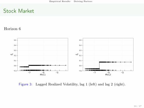
Stock Market
Horizon 6
●●● ●●●●●●●
●
●●●● ●● ●● ●●● ●
●
●
●
● ●●
●
●●● ● ●● ● ●● ● ●● ●● ●● ●● ● ●●●
●
● ● ●●● ●●● ●●●●●● ●●
●
● ●●
●
● ●● ●
●
●● ● ●●●● ●●● ●● ●●● ●●●●●●● ●
●
● ●●
●●●
●
● ●
●
●
● ●
●●●
●●●●
●●● ●● ●●●
●● ●
●
●
● ● ●
●●
●● ● ●●
●
●●● ● ●●
● ●● ●●●
●
●●●●● ●●● ● ●●●● ●● ●● ●●● ● ●● ●● ● ●●● ●●●●●●●● ● ● ●●● ●● ● ●●●●● ● ●● ●●● ●●●● ●● ●●●● ● ●● ● ●● ●●● ●●● ●● ●●●●●● ●●
●●
●
●
●●●
●
● ●
●
●
●● ●●
● ●
●●● ●●
●
● ●
●
●●●
● ●●
● ●● ●● ●
●●
●●
● ● ●●● ●● ●● ●●● ● ●● ● ●●●●● ●●●● ●●● ●●● ●●
●
−0.1
0.0
0.1
0.2
0.3
0.4
0.5
−7 −5 −3RV.L1
η t
●●●
●
●●
●●●●●●
●
●●●
●
●
●
●
●
●●
●
●
●
● ● ●●● ●●● ●
●
● ●
●
●
● ●
●
●● ●
●
●
●
● ●●
●● ●
● ●●● ●●
●
●●●●●
● ●●● ● ●●● ● ●● ●●
●
● ●
●
●●● ●
●
●
●● ●●
●
●●●●●
●●
●
● ●
●●
●●●
●
● ● ●● ● ●●●● ●●●●●●● ●● ●●● ●● ●● ●● ● ● ●●●● ● ●● ●●●● ● ●● ● ●●
●
●●●
●
●●●●
●
●●
● ●●●● ●● ●● ●●
● ● ●●
●● ● ●●● ●●●●●●●
●
● ● ●
●●
●● ● ●●●●
●
● ●● ●●● ●●●
●
●● ●●●● ● ●● ● ●● ●●● ●●● ●● ●●●
●
●
● ●●●●●●
●
●●● ● ●● ●●● ●● ● ●●●● ●●
●
● ● ●●●● ●
●
●● ●● ●● ●
●
●●●
● ● ●
●●
●● ●● ●●
●
● ●● ● ●●●●● ●●●● ●●● ●●
●
●●
−0.1
0.0
0.1
0.2
0.3
0.4
0.5
−7 −5 −3RV.L2
η t
Figure 3: Lagged Realized Volatility, lag 1 (left) and lag 2 (right).
24 / 27
Empirical Results Driving Factors
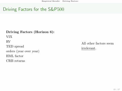
Driving Factors for the S&P500
Driving Factors (Horizon 6):VIXRVTED spreadorders (year over year)HML factorCRB returns
All other factors seemirrelevant.
25 / 27
Summary and Conclusion
• Boosting with regression trees identifies macro and financial factors thatdrive the volatility of the S&P500
• Insights into the “anatomy” of volatility:1 Identify small groups of influential drivers for stock market2 Identify volatility regimes of these drivers.3 Quantify regime dependence.
• The influence of the factors is highly nonlinear for horizon 3 and onwards.
• Forecasts for stock volatility significantly outperforms the GARCH(1,1)and EGARCH(1,1) model, especially for medium and long horizons.
26 / 27

Thank you for your attention!

References I
Audrino, F. and Bühlmann, P. (2003), “Volatility Estimation with Functional Gradient Descent forVery Highdimensional Financial Time Series,” Journal of Computational Finance, 6, 65–89.
— (2009), “Splines for Financial Volatility,” Journal of the Royal Statistical Society, Series B:Statistical Methodology, 71, 655–670.
Black, F. and Scholes, M. (1973), “The Pricing of Options and Corporate Liabilities,” Journal ofPolitical Economy, 81, 637–654.
Bühlmann, P. and Yu, B. (2003), “Boosting with the L2 Loss: Regression and Classification,”Journal of the American Statistical Association, 98, 324–339.
Freund, Y. and Schapire, R. (1996), “Experiments With a New Boosting Algorithm,” inProceedings of the Thirteenth International Conference on Machine Learning Theory, SanFrancisco: Morgan Kaufmann, pp. 148–156.
Friedman, J. H. (2001), “Greedy Function Approximation: A Gradient Boosting Machine,” TheAnnals of Statistics, 29, 1189–1232.
Lunde, A. and Hansen, P. R. (2005), “A Forecast Comparison of Volatility Models: Does AnythingBeat a GARCH(1,1)?” Journal of Applied Econometrics, 20, 873–889.
Matías, J. M., Febrero-Bande, M., González-Manteiga, W., and Reboredo, J. C. (2010), “BoostingGARCH and Neural Networks for the Prediction of Heteroskedastic Time Series,”Mathematical and Computer Modelling, 51, 256–271.
Shephard, N. and Andersen, T. G. (2009), “Stochastic Volatility: Origins and Overview,” inHandbook of Financial Time Series, eds. Mikosch, T., Kreiß, J.-P., Davis, R. A., andAndersen, T. G., Springer Berlin Heidelberg, pp. 233–254.
27 / 27