stochastic volatility and jumps in interest rates: an empirical analysis

Stochastic Volatility and Jumps in Interest Rates:An Empirical Analysis

Ren-Raw Chen* and Louis Scott**

August 2001Revised January 2002

* Rutgers University** Morgan Stanley & Co.


Abstract

Daily changes in interest rates display statistical properties that are similar to those observed inother financial time series. The distributions for changes in Eurocurrency interest rate futures areleptokurtic with fat tails and an unusually large percentage of observations concentrated at zero.The implied volatilities for at-the-money options on interest rate futures reveal evidence of sto-chastic volatility, as well as jumps in volatility. A stochastic volatility model with jumps in bothrates and volatility is fit to the daily data for futures interest rates in four major currencies and themodel provides a better fit for the empirical distributions. A method for incorporating stochasticvolatility and jumps in a complete model of the term structure is discussed.


1 Introduction

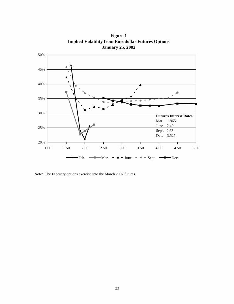
Models of the term structure of interest rates have many applications in financial man-agement. Banks that trade and make markets in interest rate derivatives use models to value andhedge their derivative portfolios. Models for the future evolution of multiple interest rates underthe risk-neutral distribution are calibrated daily for the purpose of valuation, and these models areused to implement hedging strategies. Models for changes in interest rates, under real world dis-tributions, are used to monitor market and credit risk in derivative positions. The joint distribu-tion for changes in interest rates, including the covariation across multiple maturities, is criticalfor all of these applications. A common perception in the market is that interest rates do not varymuch in the absence of economic news, but do move in response to the release of new numberson the state of the economy and to shocks in financial markets. One could argue that interest ratevolatility changes as markets react to the arrival of new information. In some cases, the swingsin interest rates, particularly short-term interest rates, have been sudden and dramatic. For exam-ple, on the day after the stock market crash of October of 1987, short-term interest rates in theU.S. dropped by more than 100 basis points as investors sought safe havens from the stock mar-ket: 3 month LIBOR dropped from 9.1875% to 8.25% and the December Eurodollar futuresprice increased from 90.64 to 91.80. In the British market, short-term interest rates dropped dra-matically during the exchange rate crisis of September 1992: on September 17, 1992, 3 monthLIBOR in pound sterling dropped from 10.062% to 9.623% after a drop of 50 basis points for theprevious day, and the December futures interest rate decreased from 10.80% to 8.72%. The mar-ket for interest rate options incorporates stochastic volatility and the potential for large interestrate moves in the form of a volatility smile, or skew. In Figure 1, we have plotted the impliedvolatility from Black’s model for the actively traded Eurodollar futures options. The variation inthe implied interest rate volatility is significant across the strikes for options with the same expi-ration date, and the slope of the skew is largest for the options with near term expirations.1 Thepurpose of this paper is to examine empirically the role of stochastic volatility and jumps inshort-term interest rates. In the last section of the paper, we use results from Duffie, Pan, andSingleton (2000) to construct a term structure model that is tractable and incorporates these em-pirical features of interest rate volatility.

1 The implied volatilities have been computed for the close on Jan. 25, 2002, and only those options with less than 1year to expiration and volumes of at least 1,000 contracts were used. The options trade at the Chicago MercantileExchange and the implied volatility is for the futures rate, not the futures price. The options are American and a lat-tice model was used to compute the American premium and the implied volatility. The early exercise premiums forthese options are small. The largest computed early exercise premium is 0.27 basis points, and the largest as a per-centage of the option value is 0.48%.

2

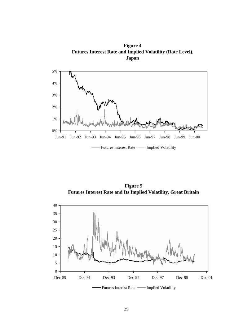
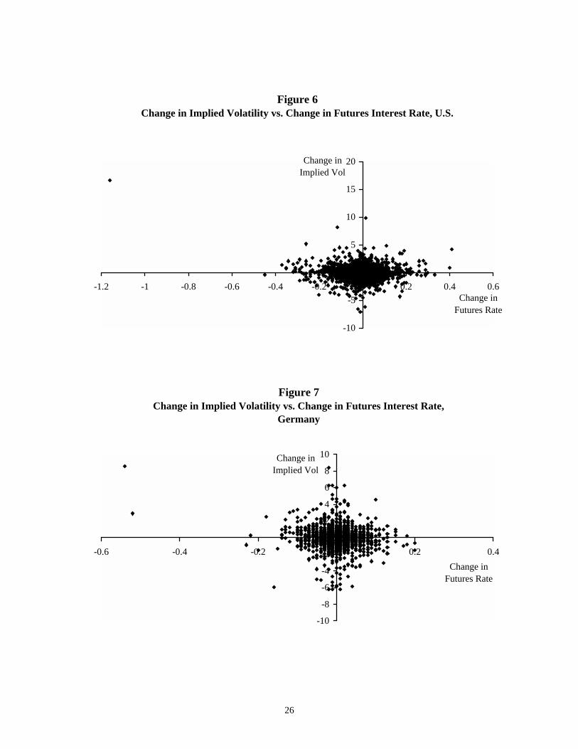
To motivate the role of stochastic volatility and jumps in interest rates, we begin with astatistical analysis of futures interest rates and implied volatilities from the markets for optionson interest rate futures. Figures 2-5 contain time series plots of the LIBOR futures interest ratesand the implied volatility for four major currencies.2 All of the contracts included here are thenear delivery futures contracts on 3 month LIBOR, or 3 month TIBOR for the Japanese yen mar-ket.3 To construct the time series, we roll to the next delivery in the quarterly cycle at the begin-ning of each delivery month. An inspection of these plots reveals that there have been days whenthere were large, sudden changes in both short-term interest rates and the implied volatility, but itshould be noted that some of the apparent jumps are associated with the roll between differentfutures contracts. Figures 6 to 9 contain scatter plots of changes in the implied volatility versuschanges in futures interest rates.4 The patterns in the scatter plots reveal some interesting fea-tures that are common across all four currencies: changes in the futures interest rates and the im-plied volatilities are randomly scattered around zero and there does not appear to be much, if any,correlation between the two variables. The plots also highlight the discrete nature of changes inthe futures rates. The tick size is one basis point for the interest rate futures in German marks(Euros), Japanese yen, and British pounds. The tick size for the U.S. dollar interest rate futureswas one basis point up until a few years ago when it was reduced to half of a basis point.

There are some extreme outliers, and it is unlikely that diffusion processes for interestrates and interest rate volatility could produce the time series in Figures 2-5 or the scatter plots inFigures 6-9. These scatter plots are also quite different from what is observed for major stockindexes. Figure 10 contains the scatter plot for changes in the CBOE volatility index (VIX) ver-sus changes in the log of the S&P 100 index. There is a strong negative correlation betweenstock price changes and changes in implied volatility, for both large changes as well as smallchanges. The correlation between price changes and volatility changes is -.67 for the S&P 100,and the rank correlation coefficient is -.63. The correlation between changes in interest rates andchanges in the implied volatility of interest rates is much smaller, and less significant: -.07 forthe U.S. rates, -.12 for Germany, .07 for Japan, and .09 for Great Britain. Several outliers associ-ated with financial shocks can be identified in the plots: the October 1987 crash for the U.S.market and the exchange rate shock in September 1992 for the pound sterling and the Europeancurrencies. If these outliers are removed, the correlation coefficients decrease significantly: .008for the U.S., -.06 for Germany, and .05 for Great Britain. The rank correlation coefficients for

2 The markets trade on futures prices with the final settlement based on 100 minus 3 month LIBOR on the deliverydate. The futures rate is 100 minus the futures price. The market convention is to quote the implied volatility as avolatility for the log of the futures interest rate.3 The data for futures rates and implied volatilities are from the exchanges: the CME for Eurodollars; LIFFE forEurosterling, Euromarks, and Euribor; TIFFE for the futures on TIBOR. The CME data are from the DRI database,the LIFFE data are from two sources, LIFFE End-of-Day Financial Products and DRI, and the TIFFE data are fromthe TIFFE web site.4 The changes for futures rates and implied volatility are computed by using the same delivery contract, and the de-livery month used for computing these changes is the nearest delivery, which is rolled to the next delivery contract atthe beginning of each delivery month.

3

changes in interest rates and changes in the implied volatility are also small: .01 for the U.S.rates, -.04 for Germany, .13 for Japan, and .01 for Great Britain. These observations suggest thatthere is little or no correlation between interest rate changes and volatility changes, and the directdependence between jumps in interest rates and jumps in volatility is also weak.

For completeness, we have included some summary statistics for the short-term interestrates of these four currencies in Tables 1-4. There are several common features across all fourcurrencies. The excess kurtosis statistics are large, and there are many days in the samples whenthe interest rates and the futures settlement rates do not change. For example, in the U.S. dollarmarket, from March 1985 to December 2000, 3 month LIBOR did not change for 36.5% of thedays and the near delivery Eurodollar futures did not change for 19.5% of the days. The autocor-relations for changes in futures rates are all close to zero, and the sample standard deviations forchanges in the futures rates are close to the sample standard deviations for changes in 3 monthLIBOR. The correlations across interest rate changes within a currency are also significant.

The distribution of interest rate changes is important for both option pricing and value-at-risk analysis. Figure 11 contains a plot of the empirical distribution for daily changes in theEurodollar futures interest rate, and Figure 12 contains the distribution for the change in the logof this rate. Both graphs include plots of normal distributions that have been fit to the data.5

Relative to the normal, the actual distributions have fatter tails and more observations closer tozero. The plots of the empirical distributions also highlight the large number of days when thereis no change and in Figure 11 the discrete nature of the rate changes, in basis points. The ex-changes compute implied volatilities for futures rates by using Black's model with at-the-moneyput and call options, and the numbers reflect the market's forward looking expectation of volatil-ity in the futures rate. If the futures rate is determined by a diffusion process with stochasticvolatility, the implied variance rate computed from at-the-money options should be a good proxyfor the expected variance over the remaining life of the option. We have also used the impliedvolatility from the previous day to compute a conditional standard deviation for daily changes inthe log of the futures rate as follows:

2501 )1Vol( Imp. )Dev( Std. ×= t-t .

Figure 13 contains a plot of the empirical distribution for the change in the log of the Eurodollarfutures rate divided by this proxy for the conditional standard deviation. The sample standarddeviation for this time series is .9820, which implies either a small upward bias in the impliedvolatility as a predictor of future volatility, or some error in the adjustment from the annualizedvolatility to a daily volatility. Figure 13 includes a plot of a normal distribution with a mean ofzero and a standard deviation of .9820, and this normal distribution does not fit the empirical

5 We have used a mean of zero and a standard deviation equal to the sample standard deviation for the observations.

4

distribution. This preliminary analysis of the data suggests that a diffusion process with stochas-tic volatility does not fit the distributions of changes in futures rates.

2 Estimating the Jump Parameters from Daily Changes in Futures Rates

The goal in this section is to fit models to the empirical distributions for the interest ratesin the four currencies described in section 1. Jump processes are rare events that are importantfor characterizing tail behavior, and the estimation of the jump parameters will require estimatorsthat incorporate the tails of the distribution over relatively short time intervals. In addition, itmay be difficult to find evidence of jumps in volatility by examining data on interest rates only.Jumps in volatility should be most apparent in option prices, measured relative to the underlyinginterest rate or futures rate. To estimate the jump parameters, we use daily changes in interestrates as well as daily changes in the option implied volatility.

One approach to this problem has been to specify a model, solve the option pricing func-tion, and develop a complex estimation strategy that utilizes data on both interest rates and optionprices. Bakshi, Cao, and Chen (1997) have taken this approach in estimating a model for theS&P 500 stock index and Bates (1996) has taken this approach in estimating models for foreignexchange rates. To apply this approach to the term structure of interest rates, one must apply themodel simultaneously to a number of interest rates and option prices. Our approach is to applysimpler econometric techniques to the daily data on futures rates and implied volatilities and testfor deviations from diffusion based models. In the final section, we describe a formal model ofthe term structure, which incorporates jumps in both rates and volatility.

We begin by specifying an ad hoc empirical model for the futures rate as follows:

22

11

)( dJdZvdtvdv

dJdZvbFRd

++−=

+=

σθκ

(1)

where v is the stochastic variance factor, 1dZ and 2dZ are Brownian motion increments, and 1dJand 2dJ are jump processes. The jump in the futures rate is a jump process with a random inten-sity parameter )(1 tJλ = )(tvdc + and a jump size distributed as a normal with zero mean and astandard deviation 1Jσ . A mean was initially included in the distribution for the jump magni-tude, but the estimates were found to be close to zero and insignificant. The estimates for c inthe random intensity parameter were also found to be close to zero and insignificant. The jumpin the stochastic variance factor is a Poisson process with intensity parameter 2Jλ and a jumpsize that is exponentially distributed with a mean 2Jµ .

5

Under the risk neutral distribution, the futures price, or the futures rate in this case, shouldbe a martingale, but these prices are not necessarily martingales under the actual or real worlddistribution. The autocorrelations for changes in futures rates reported in Tables 1-4 are all closeto zero. These results imply that past values of futures rates are not useful in the prediction ofchanges in the futures rates. One would need to examine other economic variables or determi-nistic functions of time in order to model a non-zero drift in the d FR process. Additional mod-eling of the drift for changes in the futures rate is not likely to add anything significant to the em-pirical model.

We have chosen to model the futures rate as a “normal” process with a stochastic volatil-ity, and we use the option implied volatility as a proxy for this stochastic volatility factor. If afutures price is determined by a diffusion process with fixed volatility, df = σ dZ, and the shortrate for discounting is constant, the solution for a call on the futures is

( )( )])(1[][exp])(1[2

21

2 TfK

TfKT

TfKrT NKNfeC

σσπσ

σ−−−− −−−+−= .

For an at-the-money call, f = K, and

πσ

2TeC rT−= .

The interest rate futures examined in this paper are all American, but the options traded at theLIFFE (Eurosterling, Euromarks, and the new Euribor and Eurilibor contracts) have futures stylemargining and it is not optimal to exercise these options early. For call options on futures withfutures style margining, the general option pricing solution has the following form:

[ ]( )KTfEC t −= )(,0maxˆ ,

where the expectation is taken under the risk neutral distribution, conditional on information attime t , Tt ≤ . The contracts traded in Chicago and Japan do have early exercise premiums, butthey are generally quite small for the near term expirations. We find that there is little differencebetween the implied volatilities from the European pricing model and the American pricingmodel. Black’s model applied to an at-the-money call has the following solution:

πσσσ2

])()([ 21

21 TFReTNTNFReC BrTrT −− ≈−−= .

As a result, the normal volatility for at-the-money options is approximately equal to the at-the-money implied volatility from Black’s model multiplied by the level of the futures rate. The var-

6

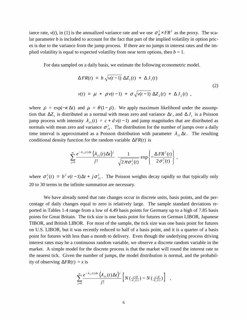
iance rate, v(t), in (1) is the annualized variance rate and we use 22 FRB ×σ as the proxy. The sca-lar parameter b is included to account for the fact that part of the implied volatility in option pric-es is due to the variance from the jump process. If there are no jumps in interest rates and the im-plied volatility is equal to expected volatility from near term options, then b = 1.

For data sampled on a daily basis, we estimate the following econometric model.

,)()()1()1()(

)()()1()(

22

11

tJtZtvtvtv

tJtZtvbtFR

∆+∆−+−+=

∆+∆−=∆

σρµ

(2)

where ρ = )exp( t∆−κ and µ = )1( ρθ − . We apply maximum likelihood under the assump-tion that 1Z∆ is distributed as a normal with mean zero and variance t∆ , and 1J∆ is a Poissonjump process with intensity )(1 tJλ = )1( −+ tvdc and jump magnitudes that are distributed asnormals with mean zero and variance 2

1Jσ . The distribution for the number of jumps over a dailytime interval is approximated as a Poisson distribution with parameter tJ ∆1λ . The resultingconditional density function for the random variable )(tFR∆ is

( )��

��

��

�� ∆−

∆�∞

=

∆−

)(2)(exp

)(21

!)(

2

2

02

1)(1

ttFR

tjtte

jj j

jJ

ttJ

σσπλλ

,

where 21

22 )1()( Jj jttvbt σσ +∆−= . The Poisson weights decay rapidly so that typically only

20 to 30 terms in the infinite summation are necessary.

We have already noted that rate changes occur in discrete units, basis points, and the per-centage of daily changes equal to zero is relatively large. The sample standard deviations re-ported in Tables 1-4 range from a low of 4.49 basis points for Germany up to a high of 7.85 basispoints for Great Britain. The tick size is one basis point for futures on German LIBOR, JapaneseTIBOR, and British LIBOR. For most of the sample, the tick size was one basis point for futureson U.S. LIBOR, but it was recently reduced to half of a basis point, and it is a quarter of a basispoint for futures with less than a month to delivery. Even though the underlying process drivinginterest rates may be a continuous random variable, we observe a discrete random variable in themarket. A simple model for the discrete process is that the market will round the interest rate tothe nearest tick. Given the number of jumps, the model distribution is normal, and the probabil-ity of observing )(tFR∆ = x is

( ) [ ]�∞

=

−+∆−

−∆

0)()(

1)(

)()(!

)(1

jt

xt

xj

Jtt

jj

J

NNj

tteσ

δσ

δλ λ

,

7

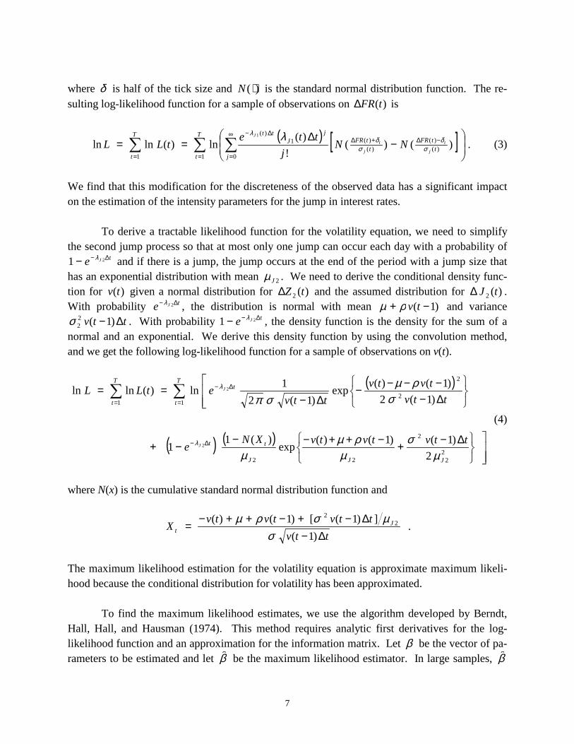
where δ is half of the tick size and )( ⋅N is the standard normal distribution function. The re-sulting log-likelihood function for a sample of observations on )(tFR∆ is

( ) [ ] .)()(!

)(ln)(lnln

1 0)(

)()(

)(1)(

1

1

� ��=

∞

=

−∆+∆∆−

=��

�

�

��

�

�−

∆==

T

t jt

tFRt

tFRj

JttT

tj

t

j

tJ

NNj

ttetLL σ

δσ

δλ λ

(3)

We find that this modification for the discreteness of the observed data has a significant impacton the estimation of the intensity parameters for the jump in interest rates.

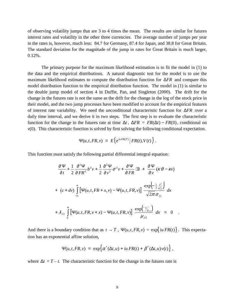
To derive a tractable likelihood function for the volatility equation, we need to simplifythe second jump process so that at most only one jump can occur each day with a probability of

tJe ∆−− 21 λ and if there is a jump, the jump occurs at the end of the period with a jump size thathas an exponential distribution with mean 2Jµ . We need to derive the conditional density func-tion for )(tv given a normal distribution for )(2 tZ∆ and the assumed distribution for )(2 tJ∆ .With probability tJe ∆− 2λ , the distribution is normal with mean )1( −+ tvρµ and variance

ttv ∆− )1(22σ . With probability tJe ∆−− 21 λ , the density function is the density for the sum of a

normal and an exponential. We derive this density function by using the convolution method,and we get the following log-likelihood function for a sample of observations on v(t).

( )

( ) ( )��

�

��

�� ∆−+−++−−

−+

��

��

∆−−−−−

�

�

∆−==

∆−

=

∆−

=��

22

2

22

2

2

11

2)1()1()(exp

)(11

)1(2)1()(exp

)1(21ln)(lnln

2

2

JJJ

tt

T

t

tT

t

ttvtvtvXNe

ttvtvtv

ttvetLL

J

J

µσ

µρµ

µ

σρµ

σπ

λ

λ

(4)

where N(x) is the cumulative standard normal distribution function and

ttvttvtvtvX J

t ∆−∆−+−++−

=)1(

])1([)1()( 22

σµσρµ

.

The maximum likelihood estimation for the volatility equation is approximate maximum likeli-hood because the conditional distribution for volatility has been approximated.

To find the maximum likelihood estimates, we use the algorithm developed by Berndt,Hall, Hall, and Hausman (1974). This method requires analytic first derivatives for the log-likelihood function and an approximation for the information matrix. Let β be the vector of pa-rameters to be estimated and let β̂ be the maximum likelihood estimator. In large samples, β̂

8

has a distribution that is approximately normal with mean β and a covariance matrix that is theinverse of the information matrix. The information matrix is estimated by computing

�=

′

��

��

�

∂∂

��

��

�

∂∂T

t

tLtL1

)(ln)(lnββ

,

and the inverse of the information matrix is used in the algorithm to find the maximum likeli-hood estimator. This approximation for the information matrix is based on the observation that

′

��

��

�

∂∂

��

��

�

∂∂=��

�

��

�

′∂∂∂−

ββββ)(ln)(ln)(ln2 tLtLEtLE .

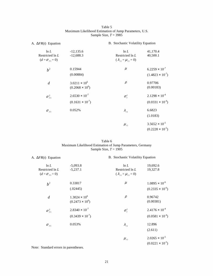
The results of the maximum likelihood estimation are summarized in Tables 5–8. All ofthe parameter estimates are large relative to their standard errors so that the parameter estimatesare statistically significant at conventional significance levels. The ρ parameters in the volatilityequations are also significantly different from one in all four samples: the t statistics for the nullhypothesis that ρ = 1 are -12.54 for volatility in U.S. rates, -8.55 for Germany, -12.94 for Japan,and -10.33 for Great Britain. These results are evidence supporting mean reversion in the im-plied volatility. The likelihood ratio statistics for testing the null hypotheses of no jumps in ratesand no jumps in volatility are all statistically significant. Each one of these statistics has an as-ymptotic distribution that is chi-squared with 2 degrees of freedom under the null hypothesis.The likelihood ratio statistics for no jumps in rates are 1,105.4 for the U.S., 286.6 for Germany,383.4 for Japan, and 450.6 for Great Britain. The likelihood ratio statistics for no jumps in vola-tility are 1,340.6 for the U.S., 729.6 for Germany, 1,166.0 for Japan, and 695.6 for Great Britain.We have also reported the estimated values for 1Jσ , the standard deviation for the magnitude ofthe interest rate jump when a jump occurs. For the U.S., the estimate of d implies an averagevalue of 206.0 for )(1 tJλ , which corresponds to an average of 206 jumps per year.6 The 1Jσ es-timate is 0.052%, or 5 basis points, for jumps in interest rates, which can be compared to thedaily standard deviation of 6.4 basis points. The estimate of 6.682 for 2Jλ implies an average of6 to 7 jumps per year in volatility. The value of 2Jµ is the expected jump size for the annualizedvariance of the change in the futures rate. The market quotes the implied volatility as an annual-ized standard deviation for FRFR∆ . For the U.S. results, if we use a futures rate of 5% and theestimated average variance level of 6.8198 ×10-5, the estimate of 3.5652×10-5 for 2Jµ implies anexpected increase of 3.86% in the annualized implied volatility when a jump in volatility is trig-gered. The exponential distribution is skewed to the right so that there is a reasonable probability

6 Here, and below, the mean for the stochastic variance process is computed from the estimates for the model in (1).The mean for the variance process includes the mean reverting level and the effect of the jump.

9

of observing volatility jumps that are 3 to 4 times the mean. The results are similar for futuresinterest rates and volatility in the other three currencies. The average number of jumps per yearin the rates is, however, much less: 84.7 for Germany, 87.4 for Japan, and 38.8 for Great Britain.The standard deviation for the magnitude of the jump in rates for Great Britain is much larger,0.12%.

The primary purpose for the maximum likelihood estimation is to fit the model in (1) tothe data and the empirical distributions. A natural diagnostic test for the model is to use themaximum likelihood estimates to compute the distribution function for FR∆ and compare thismodel distribution function to the empirical distribution function. The model in (1) is similar tothe double jump model of section 4 in Duffie, Pan, and Singleton (2000). The drift for thechange in the futures rate is not the same as the drift for the change in the log of the stock price intheir model, and the two jump processes have been modified to account for the empirical featuresof interest rate variability. We need the unconditional characteristic function for FR∆ over adaily time interval, and we derive it in two steps. The first step is to evaluate the characteristicfunction for the change in the futures rate at time t∆ , FR∆ = )0()( FRtFR −∆ , conditional onv(0). This characteristic function is solved by first solving the following conditional expectation.

( ))(),(),,,( )( tVtFReEvFRtu TFRiu=Ψ .

This function must satisfy the following partial differential integral equation:

)(021

21 2

2

22

2

2

vvFR

vv

vbFRt

κθκσ −∂Ψ∂+⋅

∂Ψ∂+

∂Ψ∂+

∂Ψ∂+

∂Ψ∂

[ ]( )

[ ] ( ).0

exp),,,(),,,(

2

exp),,,(),,,()(

0 22

1

21

2

21

2

=Ψ−+Ψ+

−Ψ−+Ψ++

�

�

∞ −

∞

∞−

dxvFRtuxvFRtu

dxvFRtuvxFRtudvc

J

x

J

J

x

J

J

µλ

σπ

µ

σ

And there is a boundary condition that as Tt → , ),,,( vFRtuΨ = { })(exp tFRiu . This expecta-tion has an exponential affine solution,

{ })(),()(),(exp),,,( ** tvuttFRiuutvFRtu ∆++∆=Ψ βα ,

where t∆ = T – t. The characteristic function for the change in the futures rate is

10

( )

{ })0(),(),(exp

),,0,()0(),0()(

**

)0()]0()([*

vutut

VFRuevFReEu iuFRFRtFRui

∆+∆=

Ψ==Φ −−∆

βα

with

)1()(2)1(),(*

t

t

eeaut ∆−

∆−

−−−−−=∆ γ

γ

κγγβ

( ) ( )

( ) ��

��

��

�

�−

−−−

+−−∆−

++∆++

∆−+��

��

��

�

�−−−+∆−−=∆

∆−

−∆−

tJ

J

J

JJ

ut

eaa

ata

t

tecetut J

γ

σγ

γµκγ

µκγµ

µκγκγλ

γκγ

σσκγκθα

12

1ln)(

2)(

112

1ln2),(

22

22

2

22

22*

2212

1

a22 σκγ += and )1(222

12122 uJeduba σ−−+= .

To get the unconditional characteristic function, we need to take the unconditional expectation of)(* uΦ :

][)]([)( )0(),(),(* ** vutut eEeuEu ∆∆=Φ=Φ βα .

This is done by evaluating first the conditional moment generating function for )( τ+tv , condi-tional on v(t) and then letting ∞→τ . This moment generating function,

])([),,( )(),(*

tveEvtuM tvut τβ +∆= ,

must satisfy the following partial differential integral equation:

[ ] { }0

exp),,(),,()(

0 222

22

21 2 =−++

∂∂+

∂∂−+

∂∂

�∞ −

dxvtuMxvtuMt

Mv

MvvMv

J

x

JJ

µλκκθσ µ .

The solution is an exponential affine function, )()()()( tveuM τβτα += , where

)1(),(2),(2)( 2*

*

κτ

κτ

σβκβκτβ −

−

−∆−∆=

eutute

11

.2),()1(),(2

)),(1(2ln

22

)1(),(22ln2)(

2*2*

*2

22

22

2*2

��

��

�

∆+−∆−∆−

−+

��

��

�

−∆−=

−−

−

J

J

J

JJ

uteeutut

eut

κµβσβκβµκ

κµσµλ

σβκκ

σκθτα

κτκτ

κτ

Let ∞→τ and the unconditional characteristic function is

( )

��

��

��

�

� −−−−

−−−∆−

++∆++�

�

��

� ∆−−

�

��

��

��

��

�

� −−−−∆−−==Φ

∆−

∆−∆

γµκγ

µκµσµλλ

µκγκγλ

κβσ

σκθ

γκγ

σκθ

σκγκθ

γ

γ

tJ

JJ

JJJ

JJ

tFRiu

eaa

t

atut

eteEu

12

1ln22

)(2

),(1ln2

12

1ln2)(exp)(

22

222

222

22

*2

2

22

.)1(),(2

),(22ln

22 22

121

*2

*2

22

22 tecut

ut uJ

J

JJ J ∆−+��

��

��

��

∆−∆−

−+ − σ

βσκβµκκ

κµσµλ

The distribution has a mean of zero and the density function is symmetric around zero. Applyingthese results, we compute the cumulative distribution function for the model by using Fourierinversion of the characteristic function. For x > 0,

�∞

∞−

− Φ−+= duiu

uexFiux )()1(

21

21)(

π ,

and for x < 0, F(x) = 1 – F(-x). The numerical integration is performed by applying the Poissonsummation formula.7

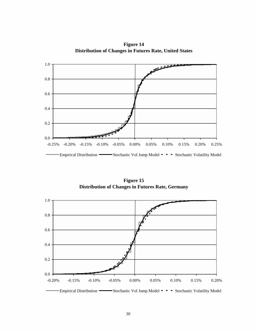
In Figures 14-17, we have plotted the empirical distribution functions with the modeldistribution functions for the stochastic volatility, jump model and the stochastic volatility modelwithout jumps. The stochastic volatility, jump model fits the empirical distribution for the inter-est rates in all four currencies. The stochastic volatility model without jumps provides a good fit

7 See Feller (1972, Chps. 15, 19) for a discussion of Fourier inversion formulas and the Poisson summation formula.An application of the Poisson summation formula in an option pricing model can be found in Chen and Scott (1995).

12

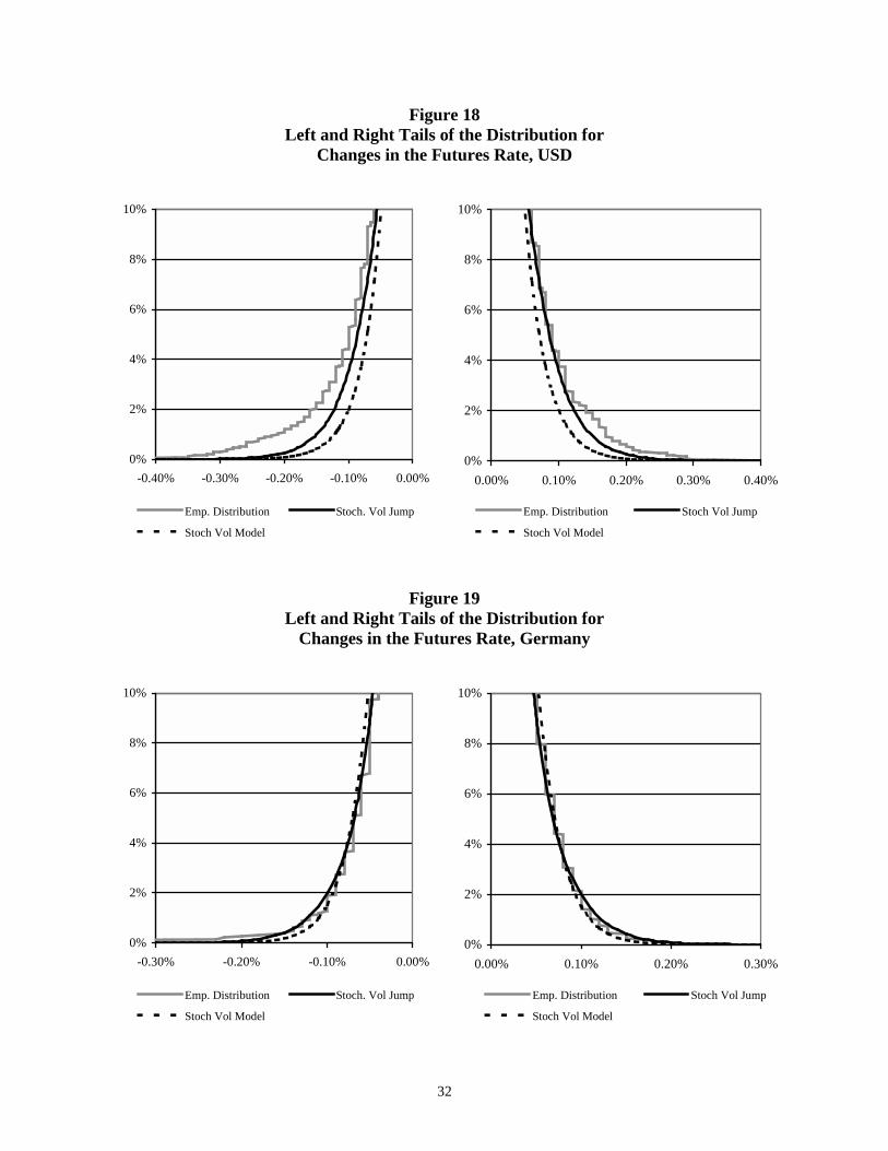
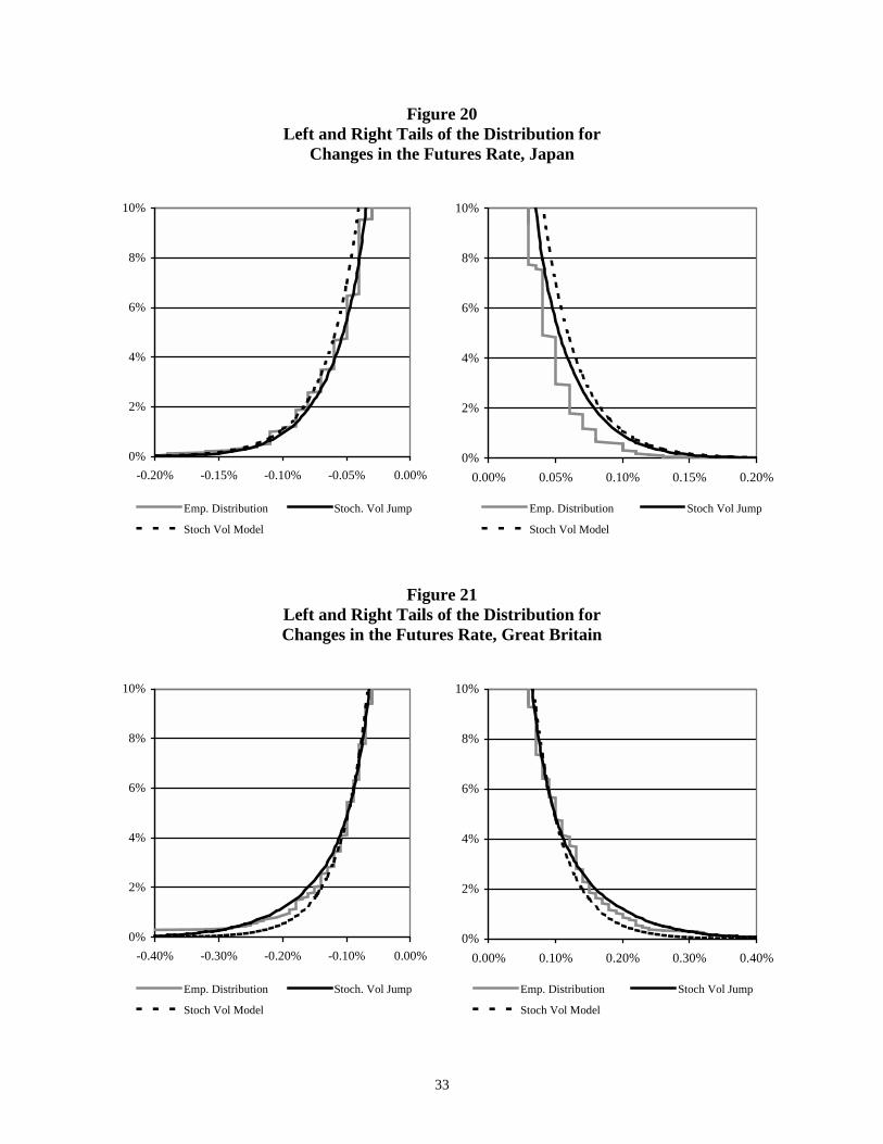
for most of the distributions, but there are noticeable deviations. The model without jumps doesnot fit the middle part of the distributions for the U.S., German, and Japanese interest rates. It is,however, difficult to distinguish the model without jumps from the stochastic volatility, jumpmodel in Figure 17 for British interest rates. There are, however, numerous extreme outliers, asshown in Figures 6-9. Figures 18-21 focus on the tails of the distribution, and here one can seethe differences between the two models, particularly in the cases of the U.S. and British interestrates. In every currency, the stochastic volatility model without jumps misses either the middlepart of the distribution or the tails of the distribution, and in some case, it misses both.

3 Summary and Extensions

The empirical analysis in section 2 highlights the importance of jumps in both interestrates and interest rate volatility. The empirical model for the analysis is an ad hoc empiricalmodel in which jump processes are added to the diffusion equations for futures interest rates. Acomplete model of the term structure of interest rates would be necessary for the management ofa portfolio of interest rate derivatives that includes options on multiple maturities. Duffie, Pan,and Singleton (2000) have recently shown how to extend exponential affine models to incorpo-rate multiple jumps, and they develop a model for valuing stock options with stochastic volatilityand simultaneous jumps in both the stock price and volatility. Their results can be used to devel-op a multi-factor model of the term structure with jumps in both interest rates and volatility. Anexample would be the following three factor model with a stochastic mean, 1y , and a stochasticvolatility, 2y :

[ ] 002010 dJdZydtrydr ++−= κκ

[ ] 11111111 dZydtydy σκθκ +−= (5)

[ ] 222222222 dJdZydtydy ++−= σκθκ

where )(tr is the instantaneous short-term interest rate.8 The two jump processes can have thesame structure as the jump processes used in the empirical model for futures rates. A model ofthis form has exponential affine solutions for discount bond prices and futures on simple interestrates such as LIBOR.9

8 See Anderson and Lund (1996) and Dai and Singleton (2000) for examples of three-factor models with stochasticmean and stochastic volatility, without the jumps.9 The solutions for a term structure model are developed in the Appendix.

13

Strategies for calibrating a model of this form are numerous. Because the bond pricingfunction and the model for futures rates are exponential affine, one can work with transforma-tions that are linear functions of the factors and develop estimators based on moments. There areanalytic solutions for the means, variances, covariances of linear combinations of the factors andone could fit the model to a set of sample moments estimated from discount rates and futuresrates. One could alternatively develop estimators based on the empirical characteristic function,as in Chacko (1999) and Singleton (2001). Another strategy would be to solve the option pricingfunctions and calibrate the model to an entire initial term structure of rates as well as optionprices for various maturities. The model could be calibrated to match an initial term structure ofinterest rates (discount rates, futures rates, and swap rates) by introducing a deterministic func-tion of time in the drift of the dr equation. To match the model to a term structure of impliedvolatilities, which is essentially a set of at-the-money option prices for different expirations, onecould make 1σ a deterministic function of time.10

Stochastic volatility and jumps are important empirical features for stock prices, foreignexchange rates, and interest rates. The empirical results presented in section 2 support the casefor stochastic volatility and jumps in interest rates, but there are some subtle, but important dif-ferences for interest rate models. There is no evidence of correlation between changes in interestrates and changes in interest rate volatility. Aside from one or two observations out of severalthousand, there is little or no evidence of correlation between large changes in interest rates andlarge changes in interest rate volatility. These results can be contrasted with the evidence ofstrong negative correlation between stock price changes and changes in stock market volatility,for both large changes and small changes.

10 In this case, the bond pricing function is still exponential affine and the deterministic function for the volatility ofthe stochastic mean factor is incorporated in the numerical solutions for the ODE’s.

14

References

Anderson, T.G., and J. Lund, “Stochastic Volatility and Mean Drift in the Short Term InterestRate Diffusion: Sources of Steepness, Level and Curvature in the Yield Curve,” North-western University, 1999.

Bakshi, G., C. Cao, and Z. Chen, “Empirical Performance of Alternative Option Pricing Mod-els,” Journal of Finance 52 (1997): 2003-49.

Bates, D., "Jumps in Stochastic Volatility: Exchange Rate Processes Implicit in Deutsche markOptions," Review of Financial Studies 9 (1996): 69-107.

Bates, D., "Post-’87 Crash Fears in S&P 500 Futures Options," Journal of Econometrics 94(2000): 181-238.

Berndt, E.K., B.H. Hall, R.E. Hall, and J.A. Hausman, “Estimation and Inference in NonlinearStructural Models,” Annals of Economic and Social Measurement 3 (1974): 653-65.

Black, F., “The Pricing of Commodity Contracts,” Journal of Financial Economics 3 (1976):167-79.

Chacko, G., “Multifactor Interest Rate Dynamics and Their Implications for Bond Pricing,” Har-vard Business School, January 1997.

_____, “Continuous-Time Estimation of Exponential Separable Term Structure Models: A Gen-eral Approach,” Harvard University, August 1999.

Chen, R.R., and L. Scott, “Pricing Interest Rate Options in a Two-Factor Cox-Ingersoll-RossModel of the Term Structure,” Review of Financial Studies 5 (1992): 613-36.

, “Interest Rate Options in Multi-Factor Cox-Ingersoll-Ross Models of the Term Struc-ture,” Journal of Derivatives 3 (Winter 1995): 53-72.

Cox, J.C., J.E. Ingersoll, and S.A. Ross, “The Relationship Between Forward and FuturesPrices,” Journal of Financial Economics 9 (December 1981): 321-46.

, “An Intertemporal General Equilibrium Model of Asset Prices,” Econometrica 53(March 1985a): 363-84.

15

, “A Theory of the Term Structure of Interest Rates,” Econometrica 53 (March 1985b):385-408.

Dai, Q., and K.J. Singleton, “Specification Analysis of Affine Term Structure Models,” (2000a),forthcoming Journal of Finance.

Dai, Q., and K.J. Singleton, “Expectation Puzzles, Time-varying Risk Premia, and DynamicModels of the Term Structure,” Stanford University, November 2000b.

Das, S., “Poisson-Gaussian Processes and the Bond Markets,” National Bureau of Economic Re-search, Working Paper 6631, July 1998.

Das, S., “Interest Rate Modeling with Jump-Diffusion Processes,” in Advanced Fixed-IncomeValuation Tools, edited by N. Jegadeesh and B. Tuckman, John Wiley & Sons, 2000.

Duffie, D., and R. Kan, “A Yield-Factor Model of Interest Rates,” Mathematical Finance 6(1996): 379-406.

Duffie, D., J. Pan, and K. Singleton “Transform Analysis and Asset Pricing for Affine Jump Dif-fusions,” Econometrica 68 (2000): 1343-76.

Embrechts, P., C. Kluppelberg, and T. Mikosch, Modeling Extremal Events for Insurance andFinance (Berlin: Springer, 1997).

Embrechts, P., A. McNeil, and D. Straumann, “Correlation and Dependence in Risk Manage-ment: Properties and Pitfalls,” to appear in Risk Management: Value at Risk and Be-yond, Cambridge University Press, 2001.

Feller, W., An Introduction to Probability Theory and Its Applications, Volume II (New York:John Wiley & Sons, 1971).

Pan, J., “The Jump-Risk Premia Implicit in Options: Evidence from an Integrated Time-SeriesStudy,” MIT Sloan School of Management, January 2001.

Scott, L., “Pricing Stock Options in a Jump-Diffusion Model with Stochastic Volatility and In-terest Rates: Applications of Fourier Inversion Methods,” Mathematical Finance 7(1997): 345-58.

Singleton, K.J., “Estimation of Affine Asset Pricing Models Using the Empirical CharacteristicFunction,” Journal of Econometrics 102 (2001): 111-141.

16

Appendix

The formal model, under the risk neutral distribution, is

[ ]

[ ]

[ ] 2222222222

111111111

00220010

)(

)(

dJdZydtydy

dZydtydy

dJdZydtyrydr

+++−=

++−=

++−−=

σλκθκ

σλκθκ

λκκ

(A1)

where )(tr is the instantaneous short-term interest rate, )(1 ty is a stochastic mean factor, and)(2 ty is a stochastic volatility factor. The jump in the short-term rate is a jump process with a

random intensity parameter )(0 tJλ ′ = )(2 tya′ and a jump size distributed as a normal with mean0Jµ′ and a standard deviation 0Jσ . The jump in the stochastic volatility factor is a Poisson proc-

ess with intensity parameter 2Jλ ′ and a jump size that is exponentially distributed with a mean2Jµ′ . The two jumps can be modeled as independent processes for interest rates, except that the

intensity of the interest rate jump is a function of 2y . The parameters with primes are jump pa-rameters that should be adjusted when moving from the real world distribution to the risk neutraldistribution.

The model in (A1) can be solved to produce a pricing function for discount bonds, as wellas futures on 3 month LIBOR. The discount bond pricing function is the solution to the follow-ing expectation under the risk-neutral distribution:

��

��

��

��−= � )(),(),()(expˆ);,,,( 2121 tytytrdssrETyyrtP

T

t .

This function must satisfy the following partial differential integral equation:

[ ]

[ ] [ ] PryyPy

yP

yryrPy

yPy

yPy

rP

tP

−+−∂∂++−

∂∂+

−−∂∂+

∂∂+

∂∂+

∂∂+

∂∂

222222

111111

2001022

22

2

21

12

21

2

21

22

2

21

)()( λκθκλκθκ

λκκσσ

17

[ ] ( ){ }

[ ] ( ).0

exp),,,(),,,(

2

exp),,,(),,,(

0 221212

0

2

21

21212

2

0

0

=′

−+′+

−−+′+

�

�

∞′

−

∞

∞−

′−

dxyyrtPxyyrtP

dxyyrtPyyxrtPya

J

x

J

J

x

J

J

J

µλ

σπ

µ

σµ

The solution for the bond pricing function is an exponential affine function of the state variables,

{ })()()()()()()(exp);,,,( 2211021 tyBtyBtrBATyyrtP ττττ −−−−= ,

where tT −=τ and the coefficients are solutions to the following system of ordinary differentialequations.

)(1 000 τκτ

BddB

−=

)()()()( 111002

1212

11 τλκτκτστ

BBBddB

+−+−=

{ }[ ]

��

��

�−

′+′−+=

−+′−′−

+−−−−=

1)(1

1)()(

1)()(exp

)()()()()(

222222111

20

202

100

22200202

122

222

12

τµλτθκτθκ

τ

στµτ

τλκτλττστ

BBB

ddA

BBa

BBBBddB

JJ

JJ

The boundary conditions are 0)0()0()0()0( 210 ==== BBBA . The first equation can be solvedanalytically:

00

01)(κ

ττκ−−= eB .

The other equations must be solved numerically.11 The continuously compounded yields for dis-count bonds, )(ln tTP −− , are linear functions of the state variables, which are useful for em-pirical analysis. 11 Standard ODE solvers, such as Runge-Kutta, produce extremely accurate solutions very quickly.

18

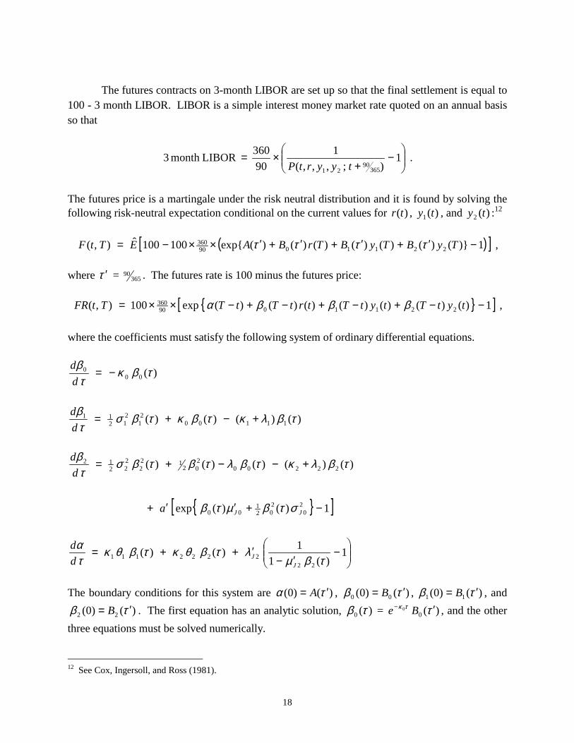
The futures contracts on 3-month LIBOR are set up so that the final settlement is equal to100 - 3 month LIBOR. LIBOR is a simple interest money market rate quoted on an annual basisso that

��

��

�−

+×= 1

);,,,(1

90360 LIBORmonth 3

36590

21 tyyrtP .

The futures price is a martingale under the risk neutral distribution and it is found by solving thefollowing risk-neutral expectation conditional on the current values for )(tr , )(1 ty , and )(2 ty :12

( )[ ]1)}()()()()()()(exp{100100ˆ),( 2211090360 −′+′+′+′××−= TyBTyBTrBAETtF ττττ ,

where τ ′ = 36590 . The futures rate is 100 minus the futures price:

{ }[ ]1)()()()()()()(exp100),( 2211090360 −−+−+−+−××= tytTtytTtrtTtTTtFR βββα ,

where the coefficients must satisfy the following system of ordinary differential equations.

)(000 τβκτβ

−=dd

)()()()( 111002

1212

11 τβλκτβκτβστβ

+−+=dd

{ }[ ]

��

��

�−

′−′++=

−+′′+

+−−+=

1)(1

1)()(

1)()(exp

)()()()()(

222222111

20

202

100

22200202

122

222

12

τβµλτβθκτβθκ

τα

στβµτβ

τβλκτβλτβτβστβ

JJ

JJ

dd

a

dd

The boundary conditions for this system are )()0( τα ′= A , )()0( 00 τβ ′= B , )()0( 11 τβ ′= B , and)()0( 22 τβ ′= B . The first equation has an analytic solution, )(0 τβ = )(0

0 ττκ ′− Be , and the otherthree equations must be solved numerically.

12 See Cox, Ingersoll, and Ross (1981).

19

Table 1Summary Statistics, U.S. LIBOR

Sample Period, March 1985 to December 2000, T = 3985

Changes in Interest RatesFutures Rate 3 Month LIBOR 6 Month LIBOR 12 Month LIBOR

Sample Mean -0.0027% -0.0010% -0.0010% -0.0012%Standard Deviation 0.0641% 0.0682% 0.0725% 0.0798%Excess Kurtosis 32.30 14.45 17.47 18.07% of Days, No Change 19.5% 36.5% 34.4% 30.5%

Autocorrelations:1 0.07 -0.09 -0.11 -0.092 0.02 0.02 0.04 0.033 -0.01 -0.02 -0.01 -0.014 -0.02 0.02 -0.01 0.00

Correlation Matrix1.00 0.38 0.41 0.430.38 1.00 0.70 0.610.41 0.70 1.00 0.720.43 0.61 0.72 1.00

Table 2Summary Statistics, German LIBOR

Sample Period, August 1990 to February 1998, T = 1898


Sample Mean 0.0000% -0.0026% -0.0027% -0.0028%Standard Deviation 0.0449% 0.0630% 0.0620% 0.0653%Excess Kurtosis 22.23 9.10 8.11 6.09% of Days, No Change 15.4% 30.5% 30.9% 30.5%

Autocorrelations:1 -0.01 -0.19 -0.24 -0.202 0.07 0.02 0.04 0.003 -0.05 -0.03 -0.03 0.004 0.03 -0.02 0.02 0.01


20

Table 3Summary Statistics, Japan TIBOR

Sample Period, July 1989 to December 2000, T = 2808


Sample Mean -0.0008% -0.0018% -0.0018% -0.0018%Standard Deviation 0.0371% 0.0353% 0.0358% 0.0357%Excess Kurtosis 9.30 15.10 11.20 10.95% of Days, No Change 21.4% 42.7% 38.9% 36.4%

Autocorrelations:1 0.08 0.14 0.12 0.162 -0.01 0.02 0.05 0.073 0.02 0.02 0.02 0.074 0.06 0.01 0.03 0.03


Table 4Summary Statistics, British LIBOR

Sample Period, August 1990 to December 2000, T = 2620


Sample Mean -0.0019% -0.0035% -0.0035% -0.0034%Standard Deviation 0.0785 0.0836% 0.0920% 0.0947%Excess Kurtosis 202.53 29.75 24.14 21.74% of Days, No Change 11.53% 28.9% 26.9% 28.0%

Autocorrelations:1 0.07 -0.23 -0.18 -0.182 -0.04 0.03 -0.02 0.013 0.09 -0.01 0.05 0.054 0.01 0.05 0.03 0.01


21

Table 5Maximum Likelihood Estimation of Jump Parameters, U.S.

Sample Size, T = 3985

A. ∆FR(t) Equation B. Stochastic Volatility Equation

ln L -12,135.6 ln L 41,170.4Restricted ln L -12,688.3 Restricted ln L 40,500.1(d = 1Jσ = 0) ( 2Jλ = 2Jµ = 0)

2b 0.15944 µ 6.2259 × 10-7

(0.00884) (1.4823 × 10-7)

d 3.0211 × 106 ρ 0.97706(0.2068 × 106) (0.00183)

21Jσ 2.6530 × 10-7 2

2σ 2.1298 × 10-4

(0.1631 × 10-7) (0.0331 × 10-4)

1Jσ 0.052%2Jλ 6.6823

(1.0183)

2Jµ 3.5652 × 10-5

(0.2228 × 10-5)

Table 6Maximum Likelihood Estimation of Jump Parameters, Germany




2b 0.33817 µ 1.0895 × 10-6

(.02445) (0.2335 × 10-6)

d 1.3024 × 106 ρ 0.96742(0.2473 × 106) (0.00381)

21Jσ 2.8340 × 10-7 2

2σ 2.4176 × 10-4

(0.3439 × 10-7) (0.0581 × 10-4)

1Jσ 0.053%2Jλ 12.896

(2.611)

2Jµ 2.0265 × 10-5

(0.0221 × 10-5)Note: Standard errors in parentheses.

22

Table 7Maximum Likelihood Estimation of Jump Parameters, Japan




2b 0.33198 µ 1.6495 × 10-6

(.02092) (0.2151 × 10-6)

D 2.7926 × 106 ρ 0.91281(0.4278 × 106) (0.00674)

21Jσ 1.7606 × 10-7 2

2σ 3.1403 × 10-4

(0.2317 × 10-7) (0.0547 × 10-4)

1Jσ 0.042%2Jλ 10.083

(1.604)

2Jµ 3.1957 × 10-5

(0.4506 × 10-5)

Table 8Maximum Likelihood Estimation of Jump Parameters, Great Britain




2b .54115 µ 1.5771 × 10-6

(.02167) (0.2996 × 10-6)

D 4.3279 × 105 ρ 0.96357(0.6178 × 105) (0.00314)

21Jσ 1.4210 × 10-6 2

2σ 3.7018 × 10-4

(0.1355 × 10-6) (0.0460 × 10-4)

1Jσ 0.119%2Jλ 5.6627

(1.0091)

2Jµ 7.5966 × 10-5

(0.8966 × 10-5)Note: Standard errors in parentheses.

23

Note: The February options exercise into the March 2002 futures.

Figure 1 Implied Volatility from Eurodollar Futures Options

January 25, 2002

20%

25%

30%

35%

40%

45%

50%

1.00 1.50 2.00 2.50 3.00 3.50 4.00 4.50 5.00

Feb. Mar. June Sept. Dec.

Futures Interest Rates:Mar. 1.965June 2.40Sept. 2.93Dec. 3.525

24

Figure 2Futures Interest Rate and Implied Volatility, United States

0

5

10

15

20

25

30

Dec-84 Dec-86 Dec-88 Dec-90 Dec-92 Dec-94 Dec-96 Dec-98 Dec-00

Futures Interest Rate Implied Volatility

Figure 3Futures Interest Rate and Its Implied Volatility, Germany

0

5

10

15

20

25

30

May-90 May-91 May-92 May-93 May-94 May-95 May-96 May-97 May-98 May-99


25

Figure 4Futures Interest Rate and Implied Volatility (Rate Level),

Japan

0%

1%

2%

3%

4%

5%

Jun-91 Jun-92 Jun-93 Jun-94 Jun-95 Jun-96 Jun-97 Jun-98 Jun-99 Jun-00


Figure 5Futures Interest Rate and Its Implied Volatility, Great Britain

0

5

10

15

20

25

30

35

40

Dec-89 Dec-91 Dec-93 Dec-95 Dec-97 Dec-99 Dec-01


26

Figure 6Change in Implied Volatility vs. Change in Futures Interest Rate, U.S.

-10

-5

0

5

10

15

20

-1.2 -1 -0.8 -0.6 -0.4 -0.2 0 0.2 0.4 0.6

Change in Implied Vol

Change inFutures Rate

Figure 7Change in Implied Volatility vs. Change in Futures Interest Rate,

Germany

-10

-8

-6

-4

-2

0

2

4

6

8

10

-0.6 -0.4 -0.2 0 0.2 0.4

Change inImplied Vol


27

Figure 8Change in Implied Volatility (Levels) vs. Change in Futures Interest Rate,

Japan

-1.40%

-0.90%

-0.40%

0.10%

0.60%

1.10%

-0.25% -0.15% -0.05% 0.05% 0.15% 0.25% 0.35%

Change in Implied Vol

Level


Figure 9Change in Implied Volatility vs. Change in Futures Interest Rate,

Great Britain

-15

-10

-5

0

5

10

-3 -2.5 -2 -1.5 -1 -0.5 0 0.5 1

Change inImplied Vol


28

Figure 10Change in VIX vs. Change in Log of S&P100 Index

-80

-60

-40

-20

0

20

40

60

80

100

120

-0.25 -0.2 -0.15 -0.1 -0.05 0 0.05 0.1

Change inVIX

Change inS&P100

Figure 11Distribution of Changes in Futures Rate, United States

0.0

0.2

0.4

0.6

0.8

1.0

-0.004 -0.003 -0.002 -0.001 0 0.001 0.002 0.003 0.004

Empirical Distribution Normal Model

29

Figure 12Distribution of Changes in Log of Futures Rate, United States

0.0

0.2

0.4

0.6

0.8

1.0

-0.06 -0.04 -0.02 0 0.02 0.04 0.06


Figure 13Distribution of Changes in Log of Futures Rate Scaled by Implied

Volatility, United States

0.0

0.2

0.4

0.6

0.8

1.0

-6 -4 -2 0 2 4 6


30

Figure 14Distribution of Changes in Futures Rate, United States

0.0

0.2

0.4

0.6

0.8

1.0

-0.25% -0.20% -0.15% -0.10% -0.05% 0.00% 0.05% 0.10% 0.15% 0.20% 0.25%

Empirical Distribution Stochastic Vol Jump Model Stochastic Volatility Model

Figure 15Distribution of Changes in Futures Rate, Germany

0.0

0.2

0.4

0.6

0.8

1.0

-0.20% -0.15% -0.10% -0.05% 0.00% 0.05% 0.10% 0.15% 0.20%


31

Figure 16Distribution of Changes in Futures Rate, Japan

0.0

0.2

0.4

0.6

0.8

1.0

-0.15% -0.10% -0.05% 0.00% 0.05% 0.10% 0.15%


Figure 17Distribution of Changes in Futures Rate, Great Britain

0.0

0.2

0.4

0.6

0.8

1.0

-0.30% -0.20% -0.10% 0.00% 0.10% 0.20% 0.30%


32

Figure 18Left and Right Tails of the Distribution for

Changes in the Futures Rate, USD


Changes in the Futures Rate, Germany

0%

2%

4%

6%

8%

10%

-0.40% -0.30% -0.20% -0.10% 0.00%

Emp. Distribution Stoch. Vol Jump

Stoch Vol Model

0%

2%

4%

6%

8%

10%

0.00% 0.10% 0.20% 0.30% 0.40%

Emp. Distribution Stoch Vol Jump

Stoch Vol Model

0%

2%

4%

6%

8%

10%

-0.30% -0.20% -0.10% 0.00%


Stoch Vol Model

0%

2%

4%

6%

8%

10%

0.00% 0.10% 0.20% 0.30%


Stoch Vol Model

33


Changes in the Futures Rate, Japan

Figure 21Left and Right Tails of the Distribution forChanges in the Futures Rate, Great Britain

0%

2%

4%

6%

8%

10%

-0.20% -0.15% -0.10% -0.05% 0.00%


Stoch Vol Model

0%

2%

4%

6%

8%

10%

0.00% 0.05% 0.10% 0.15% 0.20%


Stoch Vol Model

0%

2%

4%

6%

8%

10%

-0.40% -0.30% -0.20% -0.10% 0.00%


Stoch Vol Model

0%

2%

4%

6%

8%

10%

0.00% 0.10% 0.20% 0.30% 0.40%


Stoch Vol Model

stochastic volatility and jumps in interest rates: an empirical analysis

Documents