stochastic security-constrained unit commitment

800 IEEE TRANSACTIONS ON POWER SYSTEMS, VOL. 22, NO. 2, MAY 2007

Stochastic Security-Constrained Unit CommitmentLei Wu, Mohammad Shahidehpour, Fellow, IEEE, and Tao Li, Member, IEEE

Abstract—This paper presents a stochastic model for the long-term solution of security-constrained unit commitment (SCUC).The proposed approach could be used by vertically integrated utili-ties as well as the ISOs in electricity markets. In this model, randomdisturbances, such as outages of generation units and transmissionlines as well as load forecasting inaccuracies, are modeled as sce-nario trees using the Monte Carlo simulation method. For dual op-timization, coupling constraints among scenarios are relaxed andthe optimization problem is decomposed into deterministic long-term SCUC subproblems. For each deterministic long-term SCUC,resource constraints represent fuel and emission constraints (inthe case of vertically integrated utilities) and energy constraints(in the case of electricity markets). Lagrangian relaxation is usedto decompose subproblems with long-term SCUC into tractableshort-term MIP-based SCUC subproblems without resource con-straints. Accordingly, penalty prices (Lagrangian multipliers) aresignals to coordinate the master problem and small-scale subprob-lems. Computational requirements for solving scenario-based op-timization models depend on the number of scenarios in which theobjective is to minimize the weighted-average generation cost overthe entire scenario tree. In large scale applications, the scenario re-duction method is introduced for enhancing a tradeoff between cal-culation speed and accuracy of long-term SCUC solution. Numer-ical simulations indicate the effectiveness of the proposed approachfor solving the stochastic security-constrained unit commitment.

Index Terms—Lagrangian relaxation, mixed integer program,Monte Carlo simulation, random power outages, scenario aggrega-tion, security-constrained unit commitment, subgradient method,uncertainty.

NOMENCLATURE:

Ramp-down rate limit of unit .

Emission function of unit (type ).

Upper limit of unit ’s emission (type ).

Upper limit of group ’s emission (type).

Production cost function of unit at timeweekly interval .

Fuel consumption function of unit .

Lower fuel consumption limit of unit .

Upper fuel consumption limit of unit .

Lower fuel consumption limit of unit group.

Manuscript received June 6, 2006; revised October 1, 2006. Paper no.TPWRS-00345–2006.

The authors are with the Electrical and Computer Engineering Department,Illinois Institute of Technology, Chicago, IL 60616 USA (e-mail: [email protected]; [email protected]; [email protected]).

Digital Object Identifier 10.1109/TPWRS.2007.894843

Upper fuel consumption limit of unit group.

Index of unit.

Commitment state of unit at weeklyinterval in scenario .

Index of transmission line.

Index of unit fuel group.

Index of unit emission group.

Number of units.

Number of fuel groups.

Number of emission groups.

Number of weeks under study (52 weeks).

Number of hours at each weekly interval(168 h).

Index of weekly interval.

Weight of scenario .

Real power generation of unit at time atweekly interval in scenario .

System demand at time at weekly intervalin scenario .

Upper limit of real generation of unit .

Lower limit of real generation of unit .

Maximum capacity of line .

Power flow of line at time at weeklyinterval in scenario .

Number of scenarios.

Startup cost of unit at time at weeklyinterval in scenario .

Shutdown cost of unit at time at weeklyinterval in scenario .

Startup fuel consumption of unit at timeat weekly interval in scenario .

Shutdown fuel consumption of unit attime at weekly interval in scenario .

Startup emission of unit at time atweekly interval in scenario .

Shutdown emission of unit at time atweekly interval in scenario .

Index of time in one week.

0885-8950/$25.00 © 2007 IEEE

WU et al.: STOCHASTIC SECURITY-CONSTRAINED UNIT COMMITMENT 801

Minimum Down time of unit .

Minimum Up time of unit .

Ramp-up rate limit of unit .

On time of unit at time at weekly intervalin scenario .

On time of unit at time at weekly intervalin scenario .

Real generation vector at time at weeklyinterval in scenario .

Phase shifter angle vector at time atweekly interval in scenario .

Upper limit of phase shifter angle vector.

Lower limit of phase shifter angle vector.

I. INTRODUCTION

WITH legislative and regulatory mandates for managingelectricity restructuring, significant changes are occur-

ring in the electric power industry. Also, the electric powerbusiness is rapidly becoming market driven which is based onnodal variations of electricity prices. Meanwhile, the impact ofmarket on energy, environment, and economy requires more ef-ficient, less pollutant, and less costly means of power genera-tion by better managing resource (energy, fuel, and emission)constraints. Accordingly, long-term SCUC could be a propertool for representing interactions among resource constraintsand market objectives [1].

Our proposed stochastic model could be applied to a tra-ditional vertically integrated utility and a centralized energymarket (with ISOs). It is quite natural to model long-term fueland emission constraints for a utility as presented in this paper.In several ISOs such as PJM, MISO, and ISO-NE, SCUC is uti-lized as a market clearing tool in the day-ahead energy marketin which GENCO’s energy constraints are modeled. That is,GENCOs submit energy limits which indicate that the sum ofdaily generation for individual units, or the entire GENCO,would not exceed a prescribed level. The energy constraint isusually a linear function of GENCO’s power that is generatedby a group of units. In our proposed model, a combination offuel and emission constraints, which is a quadratic function ofpower generation by a group of units, represents the energyconstraint for a GENCO. In essence, the quadratic model thatwe are considering is more general than the existing practice ofa linear model for representing the energy limit. In this paper,we emphasize the solution of the resource based SCUC modelfor a vertically integrated utility. However, the same modelwith an energy constraint could apply to an energy market case.

The solution of long-term SCUC could become cumbersomeas we further include system uncertainties such as forced out-ages of system components and load forecasting inaccuracies.References [2], [3] used a network flow algorithm to solve thefuel dispatch problem and apply a heuristic method for unitcommitment. However, as generation constraints become morecomplicated, such a heuristic method could fail.

Decomposition is a practical method for analyzing unbun-dled electric power systems as it divides long-term SCUC into amaster problem and several tractable subproblems similar to theway the market is set up. A strategy is required to coordinate themaster problem with subproblems. Resource allocation targetsare used as linking signals to coordinate the mater problem andsubproblems for primal approaches and pseudo resource dis-patch prices for a dual approach [4]. In the primal method, themaster problem allocates long-term fuel consumption, which isdirectly used by short-term operation scheduling subproblems.The short-term solution would feed back adjustment signals forthe reallocation of long-term fuel resource constraints. Refer-ences [5], [6] used reserve capacity as a coordination indicatorbetween long-term fuel consumption allocation and short-termoptimal operation. If the available reserve capacity at any plan-ning interval was less than requested, the long-term solution wasupdated according to this violation.

Due to operating dynamics of power systems such as theoutages of generators and transmission components and uncer-tainty of system demand, the security of power systems washandled traditionally by providing spinning and operating re-serves considering the peak demand case or worst outage case.This is a conservative approach which could lead to a very highcost of operating the power system. Furthermore, outages ofmultiple components may not be considered in calculating theoperating reserve which could also lead to an insecure opera-tion of power systems. Instead of the traditional formulation ofsystem security, we propose a stochastic model in which outagesof generators and transmission components as well as uncer-tainty of system load are simulated as different scenarios. Eachscenario would represent a possible system state which wouldinclude outages of system components and a possible systemdemand. The emphasis of this paper is to simulate the impactof uncertainty and the allocation of fuel resources and emissionallowance when solving the long term stochastic security- con-strained unit commitment problem. The issue of stochastic se-curity will be explored further in our subsequent publications inwhich probabilistic indexes, such as LOLP (loss of load proba-bility) and ELNS (expected energy not served), will be used formeasuring the long-term security of power systems.

[7], [8] used a stochastic model to solve the unit commitmentproblem without considering transmission security constraints,or fuel and emission limits. [7] used fully and partially randomtrees to simulate generator failures and [8] created scenarios tosimulate generator failures and load forecasting inaccuracies.[8] modeled generator failures by creating scenarios which haddemand increases equal to the unavailable generator’s capacity;these demand increases were given by approximating the gener-ating capacity loss over a certain period of time. The advantageof the technique was its independence from individual genera-tors, but the approximation neglected the failure in geographicalinformation, and demand increases could even cause the infeasi-bility of power flows. Furthermore outages of transmission linesshould be taken into consideration.

In this paper, we model forced outages of generating unitsand transmission lines as independent Markov processes, andload forecasting uncertainties as uniform random variables. Dif-ferent scenarios are generated when stochastic conditions are


taken into account. [9] represented an efficient decompositionmethod for the solution of long-term SCUC. For each scenario,a deterministic long-term SCUC problem is solved and penaltyprice signals are used to optimize the allocation of fuel con-sumption and emission allowance based on a hybrid subgra-dient and Dantzig-Wolfe method. Lagrangian relaxation algo-rithm is adopted to deal with coupling constraints and to dividethe original problem into several tractable subproblems, i.e.,short-term SCUC based on mixed-integer program (MIP). Com-putational requirements for solving scenario-based optimizationmodels depend on the number of scenarios in which the objec-tive is to minimize the weighted-average generation cost overthe entire scenario tree. Scenario reduction is adopted in thispaper as a tradeoff between computation time and solution ac-curacy. LMPs calculated from different scenarios reflect the im-pact of uncertainties. LMPs are strongly influenced by uncer-tainties which are generally not considered in commercial soft-ware packages of SCUC. However, Fig. 9 shows that stochasticLMPs combined with their boundaries provide more accurateeconomic signals for planning and investment decisions.

The rest of the paper is organized as follows. Section II pro-vides the stochastic formulation of the uncertainty of genera-tion components (units and transmission lines) and the inac-curacy of load forecasting, discusses the scenario aggregationand scenario reduction methods. Section III presents the solu-tion methodology of the stochastic long-term SCUC. Section IVpresents and discusses two systems, a 6-bus system and a mod-ified IEEE 118-bus system with 54 units and 91 loads. The con-clusion is drawn in Section V.

II. STOCHASTIC FORMULATION

We consider a set of possible scenarios based on the MonteCarlo simulation method for modeling uncertainties in the long-term SCUC problem. Using the Monte Carlo simulation methodwe assign a weight to each scenario that reflects the possi-bility of its occurrence. The Monte Carlo simulation method,scenario aggregation, and scenario reduction technique are pre-sented in Sections II-A–C.

A. Monte Carlo Simulation Method

One of the advantages of the Monte Carlo simulation methodis the required number of samples for a given accuracy level is in-dependent of system size which makes it suitable for large scalesimulations. We use the Monte Carlo simulation method to sim-ulate the frequency and duration of generator and transmissionline outages based on forced outage rates and rates to repair.

Assume the steady state availability of the th generating unitis and its unavailability is . Using and , werepresent the th component’s repair and failure rates in the pe-riod respectively, and apply a two-state continuous-time Markovmodel for representing the th component. The associated con-ditional probabilities for component are defined as follows [6],[11]:

Fig. 1. Flowchart of a unit’s state simulation with Monte Carlo method.

We usein the Monte Carlo simulation method to simulate componentavailabilities in which indicates that the th componentis available at time t and scheduling period p while in-dicates otherwise. Fig. 1 depicts the generating unit simulationwhile a similar procedure can be devised for transmission out-ages.

A low-discrepancy Monte Carlo simulation method (lattice)is adopted with the possibility of accelerating the convergencerate from associated with ordinary Monte Carlo tonearly where is the number of sample points gener-ated. Figs. 2 and 3 represent two random number series. Pointsin Fig. 2 are generated by the ordinary Monte Carlo simulationmethod and those in Fig. 3 are generated by a rank-1 lattice rule.Accordingly, the random numbers by lattice method would bemore evenly distributed. An -point lattice rule of rank indimension is defined as follow:

where are linearly independent -vector of integers.If we draw independent samples according to the MonteCarlo simulation method, the iteration ends when the relativestandard deviation is less than a predefined value (95% relativestandard deviation is given as where is thestandard deviation and is number of simulation). Usuallyexceeds several thousands for a relatively small standard devi-ation. If the low-discrepancy method is used, convergence will


Fig. 2. Random number by Ordinary MC.

Fig. 3. Random number by Lattice.

be accelerated from to nearly and we canuse a relatively smaller number of samples to reach the sameconvergence [10].

Numerical methods have been adopted for short-term loadforecasting. However, forecasting results may be inaccurate dueto unusual changes in periodic load demands. Input data for thesimulation of outages of generators and transmission lines areforced outage rates and rates to repair, which are independentof representative days/hours in each season. For the load uncer-tainty simulation, we divide the entire scheduling horizon intoseveral time intervals. For each time interval we create a fewscenarios, based on historical data, which are different from theforecasted one. Scenarios in each time interval reflect the repre-sentative days/hours chosen for each week/season.

Here again we create multiple scenarios in which probabili-ties are assigned to occurrences. We divide the entire schedulingperiod into time units (e.g., four periods based on seasonsor several months into several weekly periods). For each timeunit we create a few scenarios (say m), based on historical data,that are different from the forecasted one. Then the scenario treewill have scenarios, each with a weight ofas shown in Fig. 4. For each scenario we solve a determin-istic long-term SCUC problem which is weighted and the finaloutcome will be an average solution for the long-term SCUC.We further combine simulation samples representing load fore-casting inaccuracies with those of component outages in a singleMonte Carlo scenario.

B. Scenario Aggregation

The idea of stochastic long-term SCUC is to construct orsample possible options for uncertain circumstances, solve thedeterministic long-term SCUC problem for the possible options,and select a good combination of outcomes to represent the sto-chastic solution.

Fig. 4. Scenario tree for the inaccurate load forecasting.

Suppose we have time periods and is a vector de-scribing time , then is a possible scenario.We create a set of scenarios S using the Monte Carlo simulationmethod where is the possibility of occurrence of . So themathematical formulation of the problem for each scenario is

S.t. system and unit constraints. Here , , and representstate variables, decision variables, and scenarios respec-tively. Accordingly, we have a number of optimal solutions

where is the number of sce-narios and the possible outcome could be the average solutionfor each time . However, averaging mayresult in a suboptimal or even infeasible solution for the originalstochastic problem [12].

Alternatively, the scenario aggregation method is formulatedas follows:

S.t.1) Original system and unit constraints for the deterministic

problem.2) Bundle constraint: if two scenarios and are indistin-

guishable from the beginning to time on the basis of in-formation available at time , then the decision renderedfor the two scenarios must be identical from the beginningto time . If represents a part of scenario s from thebeginning to time , then the bundle constraint is given as

This problem with coupling constraints for scenarios issolved using the Lagrangian relaxation method, as discussednext, with an implementable decision value defined as

C. Scenario Reduction

Computational requirements for solving scenario-based op-timization models depend on the number of scenarios. So aneffective scenario reduction method could be very essential for


solving large scale systems. The reduction technique is a sce-nario-based approximation with a smaller number of scenariosand a reasonably good approximation of original system. So wedetermine a subset of scenarios and a probability measure basedon this subset that is the closest to the initial probability distri-bution in terms of probability metrics. Our scenario reductiontechnique would control the goodness-of-fit of approximationby measuring a distance of probability distributions as a prob-ability metric. Efficient algorithms based on backward and fastforward methods are developed that determine optimal reducedmeasures. Simultaneous backward and fast forward reductionmethods are briefly introduced here as follows [14], [15]. Let

denote different scenarios, each with aprobability of , and be the distance of scenario pair

. The simultaneous backward reduction includes the fol-lowing steps:Step 1: Set is the initial set of scenarios; is the sce-

narios to be deleted. The initial are null.Compute the distances of all scenario pairs:

, ;Step 2: For each scenario , ,

and , is the scenario index that has theminimum distance with scenario .

Step 3: Compute , . Chooseso that , .

Step 4: , ; .Step 5: Repeat steps 2–4 until the number to be deleted meets

the request.The fast forward reduction method is described as follows.Step 1: Set is the set of all initial scenarios; is the

scenarios to be deleted. The initial are null.Compute the distances of all scenario pairs:

, .Step 2: Compute ,

; Choose so that ,.

Step 3: , ; ;Step 4: Repeat steps 2 to 4 until the number of scenarios to

be deleted meets the target.The General Algebraic Modeling System (GAMS) is used in

this study. GAMS provides a tool called SCENRED for sce-nario reduction and modeling random data processes. The back-ward reduction, fast forward reduction, and other methods forlarge scenario reductions are included in the SCENRED library.These scenario reduction algorithms provided by SCENREDdetermine a scenario subset (of prescribed cardinality or accu-racy) and assign optimal probabilities to the preserved scenarios[15]. The computational time for the reduction process from 100scenarios with 241 dimensions in each scenario to 12 scenariosis about five minutes. The numerical tests are executed on a 3.1GHz personal computer.

III. STOCHASTIC LONG-TERM SCUC PROBLEM

A. Stochastic Long-Term SCUC

The formulation of stochastic SCUC problem differs fromthat of deterministic since spinning and operating reserveconstraints are relaxed in the latter case. A specific amount of

spinning and operating reserves are considered in the determin-istic SCUC problem in order to maintain the security of powersystem operation when outages occur or actual hourly demandsincrease unexpectedly. In the stochastic SCUC problem, eachpossible system state is represented by a scenario in whichequipment outages and possible load increases are representedin the SCUC solution and reserve constraints are relaxed ac-cordingly. It was shown in [7] and [8] that the reserve constraintcould be relaxed because of the specific consideration of eachpotential contingency in the stochastic model. That is, a specificcommitment schedule is determined in each scenario for eachpotential contingency. In our stochastic model, we do notenforce the reserve constraint explicitly. However, it does notmean that there is no reserve in the system; reserve is implicitlydetermined by a specific commitment schedule correspondingto each potential contingency.

The Monte Carlo simulation method is adapted to simulaterandom characteristics of power systems and scenario aggrega-tion technology is used to solve the stochastic long-term SCUCproblem. A major advantage of scenario aggregation techniqueis that individual scenario problems become simple to interpret,and with aggregation technique the underlying problem struc-ture is preserved.

The objective of stochastic long-term SCUC problem is de-scribed as follows:

(1)

The objective function (1) is composed of production cost aswell as startup and shutdown costs of individual units at all pe-riods. The concept of utilizing scenarios adds another dimen-sion to the SCUC solution that is different from the determin-istic long-term SCUC solution. The generation constraints, fueland emission constraints, network security constraints, and cou-pling bundle constraints for different scenarios are presented asfollows [9], [16], [17].

Generation constraints include the system power balance

(2)

Ramping up and down constraints

(3)

Minimum up and down time constraints

(4)


Real power generation limits

(5)

Fuel constraints for individual and groups of units in aGENCO

(6)

(7)

Emission constraints for individual and groups of units in aGENCO

(8)

(9)

In a vertically integrated utility, resource (fuel consumptionand emission allowance) constraints are formulated as (8) and(9). Since the proposed method can also be applied to energymarkets (ISOs), the ISO’s energy constraint which is submittedby GENCOs will be a special case of (8) plus (9) as discussedin the introduction.

DC network security constraints (10) and phase shifter angleslimits (11)

(10)

(11)

Coupling constraints for scenarios

(12)

In (12), represents a decision part of scenario sfrom the beginning to time in the th period. Constraint (12)indicates that if two scenarios s and are indistinguishable fromthe beginning to time in the th period on the basis of infor-mation available at time , then the decision made for scenario

(here decision includes the units commitment status) must bethe same as that of scenario from the beginning to time inthe th period.

Accordingly, the objective function (1) combined with a setof constraints (2)–(12) constitutes a stochastic long-term SCUCproblem. We find that (2)–(11) are constraints that are relatedto individual scenarios and only (12) is the coupling constraintconnecting different scenarios. We solve the stochastic SCUCproblem with Lagrangian relaxation method. A Lagrangian

multiplier is associated with constraints on each .The corresponding penalty term is added tothe objective function to relax the constraint (12). Then theoriginal problem is separated into disjoint problems eachcorresponding to a scenario for deterministic long-term SCUCproblem (13) with constraints (2)–(11).

(13)

The advantages of is that it is implementable, assumedto be the weighted average of the decision made, and repre-sents an optimal solution [12]. The value of which meets

, is the same for all scenarios and givenas

The initial scenario solutions are expected to be differentbefore Lagrangian multipliers are adjusted properly. Fi-nally, scenario solutions and implementable solutionswill converge. However, since the problem is not convex, thereis no guarantee that the sequence generated by the scenario ag-gregation method would entirely converge, i.e., all scenario so-lutions and implementable solutions will be equal. Thusapproximate scenario solutions are calculated for a fast conver-gence while maintaining a relatively high accuracy as seen inthe case studies.

Starting with initial penalty multiplier , deterministiclong-term SCUC problems are solved. If the results satisfy con-straint (12), the solution is feasible and we stop. Otherwise,penalty multipliers are updated by the subgradient method andthe process is repeated as shown in Fig. 5. As discussed ear-lier, constraint (12) is not expected to be entirely satisfied. Thusbundle constraint (12) must satisfy the stopping criterion whichis stated as the weighted total violation of bundle constraints tobe below a certain threshold.

B. Deterministic Long-Term SCUC

The Lagrangian relaxation method is used for the solution ofdeterministic long-term SCUC (13) with constraints (2)–(11).Coupling constraints (6)–(9) are relaxed and dualized into theobjective function (13) with non-negative Lagrangian multi-pliers.

The relaxed coupling constraints transform the originalproblem into easier-to-solve subproblems, each of which isa traditional short-term SCUC problem at a certain periodwithout fuel and emission allowance constraints. The La-grangian relaxation problem is formulated as (14) subject toconstraints (2)–(5) and (10)–(11).

For given values of multipliers, the Lagrangian function (14)is decomposed into NP weekly short-term subproblems subject


Fig. 5. Flowchart of stochastic long-term SUCU problem.

to constraints (2)–(5) and (10)–(11). Here, we consider thelinkage of successive weekly intervals for constraints (3) and(4). Accordingly, the short-term SCUC for the first week issolved by a MIP-based method which provides the initial statusfor the short-term SCUC in the second week, and so on. See(14) at the bottom of the page.

Various methods could be applied to solve the Lagrangiandual problem. [9] presents an efficient hybrid method basedon subgradient and Dantzig-Wolfe decomposition for the so-lution of deterministic long-term SCUC problem. The hybrid

method is adopted to achieve the tradeoff between calculationspeed and exact solution. It divides the original problem into amaster problem and several subproblems. Long-term fuel andemission constraints are considered in the master problem ascoupling constraints over a schedule horizon, pseudo penaltyprice signals for fuel and emission are calculated and used di-rectly by sub-problems. The sub-problem solutions would feedback adjustment signals for the reallocation of long-term fueland emission constraints. The numerical examples presented inSection IV will show that an appropriate and near-optimal so-lution is achieved based on our proposed simulation method forthe long-term power system operation.

IV. NUMERICAL EXAMPLES

A 6-bus system, the IEEE 118-bus system, and an 1168-bussystem are considered in this section to demonstrate the pro-posed approach for solving the stochastic long-term SCUC withmultiple fuel and emission constraints in which the impact ofequipment outages and load uncertainties are included.

A. The 6-Bus System

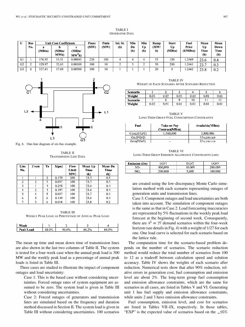
The 6-bus system in Fig. 6 is used to illustrate the proposedmethod. The system has three units and seven transmission linesas shown in Tables I and II. Unit 1 is coal-fired while unit 2 and3 are oil-fired and gas-fired, respectively. The last two columnsin Table I give the mean up time and mean down time of threeunits, which show that the larger the generating capacity, themore frequent is the generating unit’s outage.

The forced outage rate of a generation unit is calculatedas .

(14)


TABLE IGENERATOR DATA

Fig. 6. One-line diagram of six-bus example.

TABLE IITRANSMISSION LINE DATA

TABLE IIIWEEKLY PEAK LOAD AS PERCENTAGE OF ANNUAL PEAK LOAD

The mean up time and mean down time of transmission linesare also shown in the last two columns of Table II. The systemis tested for a four-week case when the annual peak load is 300MW and the weekly peak load as a percentage of annual peakloads is listed in Table III.

Three cases are studied to illustrate the impact of componentoutages and load uncertainty:

Case 1: This is the based case without considering uncer-tainties. Forced outage rates of system equipment are as-sumed to be zero. The system load is given in Table IIIwithout considering uncertainties.Case 2: Forced outages of generators and transmissionlines are simulated based on the frequency and durationmethod discussed in Section II. The system load is given inTable III without considering uncertainties. 100 scenarios

TABLE IVWEIGHT OF EACH SCENARIO AFTER SCENARIO REDUCTION

TABLE VLONG-TERM GROUP FUEL CONSUMPTION CONSTRAINTS

TABLE VILONG-TERM GROUP EMISSION ALLOWANCE CONSTRAINTS (LBS)

are created using the low-discrepancy Monte Carlo simu-lation method with each scenario representing outages ofgeneration units and transmission lines.Case 3: Component outages and load uncertainties are bothtaken into account. The simulation of component outagesis the same as that in Case 2. Load forecasting inaccuraciesare represented by 5% fluctuations in the weekly peak loadforecast at the beginning of second week. Consequently,there are demand scenarios within the four-weekhorizon (see details in Fig. 4) with a weight of 1/27 for eachone. One load curve is selected for each scenario based onthe lattice rule.

The computation time for the scenario-based problem de-pends on the number of scenarios. The scenario reductionmethod would reduce the total number of scenarios from 100to 12 as a tradeoff between calculation speed and solutionaccuracy. Table IV shows the weights of each scenario afterreduction. Numerical tests show that after 90% reduction, rel-ative errors in generation cost, fuel consumption and emissionlevel are about 2%. The long-term group fuel consumptionand emission allowance constraints, which are the same forscenarios in all cases, are listed in Tables V and VI. Generatingunit 1 has fuel supply and emission allowance constraints,while units 2 and 3 have emission allowance constraints.

Fuel consumption, emission level, and cost for scenariosare listed in Tables VII–IX, respectively. In those tables,“EXP” is the expected value of scenarios based on the


TABLE VIIRESULTS OF BASE CASE (CASE 1)

TABLE VIIIFUEL CONSUMPTION FOR EACH SCENARIO OF CASE 2

TABLE IXEMISSION LEVEL OF CASE 2

confidence interval. The “Relative Error” is calculated as.

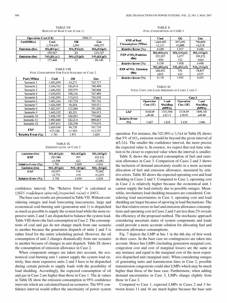
The base case results are presented in Table VII. Without con-sidering outages and load forecasting inaccuracies, large andeconomical coal-burning unit (generation unit 1) is dispatchedas much as possible to supply the system load while the more ex-pensive units 2 and 3 are dispatched to balance the system load.Table VIII shows the fuel consumption in Case 2. The consump-tions of coal and gas do not change much from one scenarioto another because the generation dispatch of units 1 and 3 israther fixed for the entire scheduling period. However, the oilconsumption of unit 2 changes dramatically from one scenarioto another because of changes in unit dispatch. Table IX showsthe consumption of emission allowance in Case 2.

When component outages are taken into account, the eco-nomical coal-burning unit 1 cannot supply the system load en-tirely, thus more expensive units 2 and 3 have to be dispatchedduring certain periods to supply loads with the possibility ofload shedding. Accordingly, the expected consumption of oiland gas in Case 2 are higher than those in Case 1. The valuesin Table IX show the emission consumption in 95% confidenceintervals which are calculated based on scenarios. The 95% con-fidence interval would reflect the uncertainty of power system

TABLE XFUEL CONSUMPTION OF CASE 3

TABLE XITOTAL COST AND LOAD SHEDDING IN CASES 2 AND 3

operation. For instance, the in Table IX showsthat 5% of emission would be beyond the given interval of

. The smaller the confidence interval, the more precisethe expected value is. In essence, we expect that real time solu-tion to be closer to expected value when the interval is smaller.

Table X shows the expected consumption of fuel and emis-sion allowance in Case 3. Comparison of Cases 2 and 3 showsthe inclusion of demand uncertainty results in a more accurateallocation of fuel and emission allowance, measured by rela-tive errors. Table XI shows the expected operating cost and loadshedding in Cases 2 and 3. Compared to Case 1, operating costin Case 2 is relatively higher because the economical unit 1cannot supply the load entirely due to possible outages. Mean-while, involuntary load shedding measures are considered. Con-sidering load uncertainties in Case 3, operating cost and loadshedding are larger because of upswing in load fluctuations. Thefact that relative errors in fuel and emission allowance consump-tions and operating cost in Cases 2 and 3 are less than 2% revealsthe efficiency of the proposed method. The stochastic approachconsidering uncertain states of system components and loadscould provide a more accurate solution for allocating fuel andemission allowance consumptions.

Fig. 7 depicts the LMP at bus 1 in the 6th day of first weekin three cases. In the base case no contingencies are taken intoaccount. Hence bus LMPs (including generation marginal cost,congestion cost and cost of marginal losses) are the same atany instance and equal to the marginal cost of the most expen-sive dispatched unit (marginal unit). When considering outagesof generating units and transmission lines in Case 2, possibletransmission congestions could alter LMPs which may be muchhigher than those of the base case. Furthermore, when addingdemand uncertainties in Case 3, LMPs change slightly fromthose in Case 2.

Compared to Case 1, expected LMPs in Cases 2 and 3 be-tween hours 11 and 16 are much higher because the base unit


Fig. 7. LMPs of bus 1 in the 6th day of the first week.

(coal-fired unit 1 with a minimum off time of 4 h) is not availableat hour 12 and will remain off until hour 16, and transmissionlines 1–2 and 2–4 are on outage at hours 15 and 16. The conges-tion is incurred at line 1–4, so the LMPs are much higher thanthose of the base case during hour 11 to 16. In spite of high loadshedding cost (set at around $1000 which are much higher thanthe generating dispatch cost), load shedding will be necessaryfor managing the security. This example is the tradeoff betweensecurity and economics as we take stochastic characteristics ofpower systems into consideration.

In each scenario, a deterministic long-term SCUC problem issolved in ten iterations for managing long-term fuel and emis-sion allowance constraints. The outer iteration is repeated fivetimes to meet the scenario bundle constraints. The CPU timeconsumed for the total twelve scenarios is about 3.6 h on a3.1-HGz personal computer. However, parallel computing usedfor each scenario, could reduce the CPU time to that of solvinga single deterministic long-term problem. If outer iterations forscenario bundle constraints are taken into account, the requiredCPU time is that of solving one deterministic long-term problemmultiplied by the outer iteration number.

B. 118-Bus System

A modified IEEE 118-bus system in Fig. 8 is used in thiscase. The test data for the 118-bus system are given at http://motor.ece.iit.edu/data/ltscuc. The system is tested in an eight-week case study to demonstrate the stochastic long-term SCUCsolution with multiple fuel and emission constraints.

The annual peak load of the system is 6,000 MW and theweekly peak load is listed in Table XII as a percentage of annualpeak load. The fuel and emission groups are listed in Table XIII.Generating units, which are burning coal, oil and gas, are rep-resented as fuel group (FGroup) 1, 2, and 3 respectively, andgenerating units with emission constraints are listed in emissiongroups (EGroup) 1, 2 and 3. The coal fuel group has upper andlower fuel supply constraints, while the oil fuel group has theupper limit fuel constraint, and the gas fuel group has the lowerlimit fuel constraint. The entire fuel consumption and emissionallowance constraints over eight weeks, which are the same fordifferent scenarios, are listed in Tables XIV and XV.

The low-discrepancy Monte Carlo simulation method is usedto create 100 scenarios, each representing possible componentoutages and load forecasting inaccuracies. The simulation ofcomponent outages is based on the frequency and duration

Fig. 8. One-line diagram of IEEE 118-bus system.

TABLE XIIWEEKLY PEAK LOAD AS PERCENTAGE OF ANNUAL PEAK LOAD

TABLE XIIIFUEL AND EMISSION GROUPS

TABLE XIVLONG-TERM GROUP FUEL CONSUMPTION CONSTRAINTS

TABLE XVLONG-TERM GROUP EMISSION ALLOWANCE CONSTRAINTS

method given in Section II. Load forecasting inaccuracies arerepresented by 5% fluctuations in weekly peak load forecastat the beginning of second week. Consequently, there are

demand scenarios within the eight-week horizon(see details in Fig. 4). Each has a weight of 1/2187. For eachscenario one load curve is selected based on the lattice rule.


TABLE XVIWEIGHTS OF EACH SCENARIO AFTER SCENARIO REDUCTION

TABLE XVIIEMISSION LEVEL

TABLE XVIIIFUEL CONSUMPTION

TABLE XIXWEEKLY PEAK LOAD

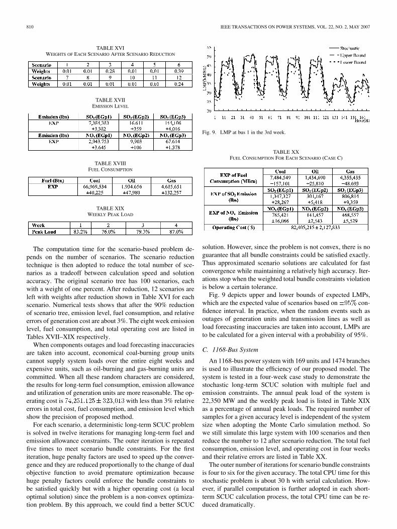
The computation time for the scenario-based problem de-pends on the number of scenarios. The scenario reductiontechnique is then adopted to reduce the total number of sce-narios as a tradeoff between calculation speed and solutionaccuracy. The original scenario tree has 100 scenarios, eachwith a weight of one percent. After reduction, 12 scenarios areleft with weights after reduction shown in Table XVI for eachscenario. Numerical tests shows that after the 90% reductionof scenario tree, emission level, fuel consumption, and relativeerrors of generation cost are about 3%. The eight week emissionlevel, fuel consumption, and total operating cost are listed inTables XVII–XIX respectively.

When components outages and load forecasting inaccuraciesare taken into account, economical coal-burning group unitscannot supply system loads over the entire eight weeks andexpensive units, such as oil-burning and gas-burning units arecommitted. When all these random characters are considered,the results for long-term fuel consumption, emission allowanceand utilization of generation units are more reasonable. The op-erating cost is with less than 3% relativeerrors in total cost, fuel consumption, and emission level whichshow the precision of proposed method.

For each scenario, a deterministic long-term SCUC problemis solved in twelve iterations for managing long-term fuel andemission allowance constraints. The outer iteration is repeatedfive times to meet scenario bundle constraints. For the firstiteration, huge penalty factors are used to speed up the conver-gence and they are reduced proportionally to the change of dualobjective function to avoid premature optimization becausehuge penalty factors could enforce the bundle constraints tobe satisfied quickly but with a higher operating cost (a localoptimal solution) since the problem is a non-convex optimiza-tion problem. By this approach, we could find a better SCUC

Fig. 9. LMP at bus 1 in the 3rd week.

TABLE XXFUEL CONSUMPTION FOR EACH SCENARIO (CASE C)

solution. However, since the problem is not convex, there is noguarantee that all bundle constraints could be satisfied exactly.Thus approximated scenario solutions are calculated for fastconvergence while maintaining a relatively high accuracy. Iter-ations stop when the weighted total bundle constraints violationis below a certain tolerance.

Fig. 9 depicts upper and lower bounds of expected LMPs,which are the expected value of scenarios based on con-fidence interval. In practice, when the random events such asoutages of generation units and transmission lines as well asload forecasting inaccuracies are taken into account, LMPs areto be calculated for a given interval with a probability of 95%.

C. 1168-Bus System

An 1168-bus power system with 169 units and 1474 branchesis used to illustrate the efficiency of our proposed model. Thesystem is tested in a four-week case study to demonstrate thestochastic long-term SCUC solution with multiple fuel andemission constraints. The annual peak load of the system is22,350 MW and the weekly peak load is listed in Table XIXas a percentage of annual peak loads. The required number ofsamples for a given accuracy level is independent of the systemsize when adopting the Monte Carlo simulation method. Sowe still simulate this large system with 100 scenarios and thenreduce the number to 12 after scenario reduction. The total fuelconsumption, emission level, and operating cost in four weeksand their relative errors are listed in Table XX.

The outer number of iterations for scenario bundle constraintsis four to six for the given accuracy. The total CPU time for thisstochastic problem is about 30 h with serial calculation. How-ever, if parallel computation is further adopted in each short-term SCUC calculation process, the total CPU time can be re-duced dramatically.


V. CONCLUSIONS

In this paper, we proposed a stochastic long-term SCUC for-mulation for representing uncertainties in the availability of gen-eration units and transmission lines, and inaccuracies in loadforecasting. The component outages are simulated by the MonteCarlo simulation. Lagrangian relaxation is applied to decom-pose the stochastic problem into many deterministic long-termSCUC sub-problems which are solved by a hybrid method. Nu-merical results show that the efficiency of the proposed solu-tion approach and the impact of outages of system componentsand demand uncertainties on system operating costs and alloca-tions of energy allocation, fuel consumption, and emission al-lowance. The merits of proposed temporal model are featuredby the simulation of uncertainties in the solution of stochasticlong-term SCUC. The stochastic solution provides more reliabledecisions on energy allocation, fuel consumption, emission al-lowance, and long-term utilization of generating units.

REFERENCES

[1] M. Shahidehpour, Y. Fu, and T. Wiedman, “Impact of natural gasinfrastructure on electric power systems,” Proc. IEEE, vol. 93, pp.1042–1056, May 2005.

[2] A. B. R. Kumar, S. Vemuri, L. A. Gibs, D. F. Hackett, and J. T. Eisen-hauer, “Fuel resource scheduling, part III, the short-term problem,”Power App. Syst., vol. PAS-103, no. 7, pp. 1556–1561, Jul. 1984.

[3] A. B. R. Kumar, S. Vemuri, L. P. Ebrahimzadeh, and N. Farah-bakhshian, “Fuel resource scheduling, the long-term problem,” IEEETrans. Power Syst., vol. PWRS-1, pp. 145–151, Nov. 1986.

[4] J. Gardner, W. Hobbs, F. N. Lee, E. Leslie, D. Streiffert, and D. Todd,“Summary of the panel session ’Coordination between short-term oper-ation scheduling and annual resource allocations’,” IEEE Trans. PowerSyst., vol. 10, pp. 1879–1889, Nov. 1995.

[5] M. Shahidehpour and M. Marwali, Maintenance Scheduling in Re-structured Power Systems. Norwell, MA: Kluwer, 2000.

[6] M. K. C. Marwali and M. Shahidehpour, “Coordination between long-term and short-term generation scheduling with network constraints,”IEEE Trans. Power Syst., vol. 15, pp. 1161–1167, Aug. 2000.

[7] P. Carpentier, G. Cohen, J. C. Culioli, and A. Renaud, “Stochastic op-timization of unit commitment: A New decomposition framework,”IEEE Trans. Power Syst., vol. 11, pp. 1067–1073, May 1996.

[8] S. Takriti, J. R. Birge, and E. Long, “A stochastic model for theunit commitment problem,” IEEE Trans. Power Syst., vol. 11, pp.1497–1508, Aug. 1996.

[9] Y. Fu, M. Shahidehpour, and Z. Li, “Long-term security constrainedunit commitment: Hybrid Dantzig-Wolfe decomposition and subgra-dient approach,” IEEE Trans. Power Syst., vol. 20, pp. 2093–2106, Nov.2005.

[10] P. Glasserman, Monte Carlo Simulation Method in Financial Engi-neering. New York: Springer, 2003.

[11] J. lenzuela and M. Mazumdar, “Monte Carlo computation of powergeneration production costs under operating constraints,” IEEE Trans.Power Syst., vol. 16, pp. 671–677, Nov. 2001.

[12] P. Kall and S. W. Wallace, Stochastic Programming. New York:Wiley, 1994.

[13] R. T. Rockafellar and R. J.-B. Wets, “Scenarios and policy aggregationin optimization under uncertainty,” Math. Oper. Res., vol. 16, no. 1, pp.119–147, 1991.

[14] J. Dupacová, N. Gröwe-Kuska, and W. Römisch, “Scenario reductionin stochastic programming: An approach using probability metrics,”Math. Programm., vol. A 95, pp. 493–511, 2003.

[15] GAMS/SCENRED Documentation [Online]. Available: www.gams.com/docs/document.htm

[16] Z. Li and M. Shahidehpour, “Generation scheduling with thermal stressconstraints,” IEEE Trans. Power Syst., vol. 18, pp. 1402–1409, Nov.2003.

[17] M. Shahidehpour, H. Yamin, and Z. Y. Li, Market Operations in Elec-tric Power Systems. New York: Wiley, 2002.

Lei Wu received the B.S. and M.S. degrees in electrical engineering from Xi’anJiaotong University, China, in 2001 and 2004, respectively. He is pursuing thePh.D. degree at Illinois Institute of Technology, Chicago.

His research interests include power systems restructuring and reliability.

Mohammad Shahidehpour (F’01) is with the Computer Engineering Depart-ment, Illinois Institute of Technology (IIT), Chicago. He is the author of 300technical papers and four books on electric power systems planning, operation,and control. His books include Maintenance Scheduling in Restructured PowerSystems (Norwell, MA: Kluwer, 2000), Restructured Electrical Power Systems(New York: Marcel Dekker, 2001), Market Operations in Electric Power Sys-tems (New York: Wiley, 2002), and Communication and Control of ElectricPower Systems (New York: Wiley, 2003).

Dr. Shahidehpour is the recipient of the 2004 IEEE Power System OperationCommittee’s Best Paper Award, 2005 IEEE/PES Best Paper Award, theEdison Electric Institute’s Outstanding Faculty Award, HKN’s OutstandingYoung Electrical Engineering Award, Sigma Xi’s Outstanding ResearcherAward, IIT’s Outstanding Faculty Award, and the University of Michigan’sOutstanding Teaching Award.

Tao Li (M’06) received the B.S. and M.S. degrees in electrical engineering fromShanghai Jiaotong University, Shanghai, China, and the Ph.D. degree from theIllinois Institute of Technology, Chicago, in 1999, 2002, and 2006, respectively.

He is currently a Senior Research Associate in the Electric Power and PowerElectronics Center, Electrical and Computer Engineering Department, IllinoisInstitute of Technology. His research interests include power system economicsand optimization.

stochastic security-constrained unit commitment

Documents