stochastic processes: learning the languageandrewc/papers/fass.pdf · stochastic processes:...
TRANSCRIPT

1
STOCHASTIC PROCESSES: LEARNING THE LANGUAGE
By A. J. G. Cairns, D. C. M. Dickson, A. S. Macdonald,
H. R. Waters and M. Willder
abstract
Stochastic processes are becoming more important to actuaries: they underlie much of mod-ern finance, mortality analysis and general insurance; and they are reappearing in the actuarialsyllabus. They are immensely useful, not because they lead to more advanced mathematics(though they can do that) but because they form the common language of workers in manyareas that overlap actuarial science. It is precisely because most financial and insurance risksinvolve events unfolding as time passes that models based on processes turn out to be mostnatural. This paper is an introduction to the language of stochastic processes. We do not giverigorous definitions or derivations; our purpose is to introduce the vocabulary, and then surveysome applications in life insurance, finance and general insurance.
keywords
Financial Mathematics; General Insurance Mathematics; Life Insurance Mathematics; Stochas-tic Processes
authors’ addresses
A. J. G. Cairns, M.A., Ph.D., F.F.A., Department of Actuarial Mathematics and Statistics,Heriot-Watt University, Edinburgh EH14 4AS, U.K. Tel: +44(0)131-451-3245; Fax: +44(0)131-451-3249; E-mail: [email protected]. C. M. Dickson, B.Sc., Ph.D., F.F.A., F.I.A.A., Centre for Actuarial Studies, The University ofMelbourne, Parkville, Victoria 3052, Australia. Tel: +61(0)3-9344-4727; Fax: +61-3-9344-6899;E-mail: [email protected]. S. Macdonald, B.Sc., Ph.D., F.F.A., Department of Actuarial Mathematics and Statistics,Heriot-Watt University, Edinburgh EH14 4AS, U.K. Tel: +44(0)131-451-3209; Fax: +44(0)131-451-3249; E-mail: [email protected]. R. Waters, M.A., D.Phil., F.I.A., F.F.A., Department of Actuarial Mathematics and Statis-tics, Heriot-Watt University, Edinburgh EH14 4AS, U.K. Tel: +44(0)131-451-3211; Fax: +44(0)131-451-3249; E-mail: [email protected]. Willder, B.A., F.I.A., Department of Actuarial Mathematics and Statistics, Heriot-WattUniversity, Edinburgh EH14 4AS, U.K. Tel: +44(0)131-451-3204; Fax: +44(0)131-451-3249;E-mail: [email protected]
1. Introduction
In Sections 2 and 3 of this paper we introduce some of the main concepts in stochasticmodelling, now included in the actuarial examination syllabus as Subject 103. In Sections4, 5 and 6 we illustrate the application of these concepts to life insurance mathematics(Subjects 104 and 105), finance (Subject 109) and risk theory (Subject 106). Subject 103includes material not previously included in the UK actuarial examinations. Hence, wehope this paper will be of interest not only to students preparing to take Subject 103, butalso to students and actuaries who will not be required to take this Subject.
It is assumed that the reader is familiar with probability and statistics up to the levelof Subject 101.
Stochastic Processes: Learning the Language 2
2. Familiar Territory
Consider two simple experiments:(a) spinning a fair coin; or(b) rolling an ordinary six sided die.
Each of these experiments has a number of possible outcomes:(a) the possible outcomes are H (heads) and T (tails); and(b) the possible outcomes are 1, 2, 3, 4, 5 and 6.
Each of these outcomes has a probability associated with it:(a) P[H] = 0.5 = P[T]; and(b) P[1] = 1
6= . . . = P[6].
The set of possible outcomes from experiment (a) is rather limited compared to thatfrom experiment (b). For experiment (b) we can consider more complicated events, eachof which is just a subset of the set of all possible outcomes. For example, we could considerthe event even number, which is equivalent to 2, 4, 6, or the event less than or equalto 4, which is equivalent to 1, 2, 3, 4. Probabilities for these events are calculated bysumming the probabilities of the corresponding individual outcomes, so that:
P[even number] = P[2] + P[4] + P[6] = 3× 1
6=
1
2
A real valued random variable is a function which associates a real number witheach possible outcome from an experiment. For example, for the coin spinning experimentwe could define the random variable X to be 1 if the outcome is H and 0 if the outcomeis T.
Now suppose our experiment is to spin our coin 100 times. We now have 2100 possibleoutcomes. We can define events such as the first spin gives Heads and the second spingives Heads and, using the presumed independence of the results of different spins, wecan calculate the probability of this event as 1
2× 1
2= 1
4.
Consider the random variable Xn, for n = 1, 2, . . . , 100 which is defined to be thenumber of Heads in the first n spins of the coin. Probabilities for Xn come from thebinomial distribution, so that:
P[Xn = m] =
(n
m
)×
(1
2
)m
×(
1
2
)n−m
for m = 0, 1, . . . , n.
We can also consider conditional probabilities for Xn+k given the value of Xn. Forexample:
P[X37 = 20 | X36 = 19] =1
2
P[X37 = 19 | X36 = 19] =1
2P[X37 = m | X36 = 19] = 0 if m 6= 19, 20.

Stochastic Processes: Learning the Language 3
From these probabilities we can calculate the conditional expectation of X37 giventhat X36 = 19. This is written E[X37 | X36 = 19] and its value is 19.5. If we had notspecified the value of X36, then we could still say that E[X37 | X36] = X36 + 1
2. There are
two points to note here:(a) E[X37 | X36] denotes the expected value of X37 given some information about what
happened in the first 36 spins of the coin; and(b) E[X37 | X36] is itself a random variable whose value is determined by the value taken
by X36. In other words, E[X37 | X36] is a function of X36.
The language of elementary probability theory has been adequate for describing theideas introduced in this section. However, when we consider more complex situations, wewill need a more precise language.
3. Further Concepts
3.1 Probability TriplesConsider any experiment with uncertain outcomes, for example spinning a coin 100
times. The mathematical shorthand (Ω,F , P) is known as a probability triple. Thethree parts of (Ω,F , P) are the answers to three very important questions relating to theexperiment, namely:(a) What are the possible outcomes of the experiment?(b) What information do we have about the outcome of the experiment?(c) What is the underlying probability of each outcome occurring?
We start by explaining the use and meaning of the terminology (Ω,F , P).
3.2 Sample SpacesThe sample space Ω is the set of all the possible outcomes, ω, of the experiment.
We call each outcome a sample point. In an example of rolling a 6 sided die the samplespace is simply:
Ω = 1, 2, 3, 4, 5, 6
In this case there are 6 sample points. We express the outcome of a 4 being rolled asω = 4.
An event is a subset of the sample space. In our example the event of an odd numberbeing rolled is the subset 1, 3, 5.
3.3 σ-algebrasWe denote by F the set of all events in which we could possibly be interested.
To make the mathematics work, we insist that F contains the empty set ∅, the wholesample space Ω, and all unions, intersections and complements of its members. Withthese conditions, F is called a σ-algebra of events1.
1To be more precise, the number of unions and intersections should be finite or countably infinite.
Stochastic Processes: Learning the Language 4
A sub-σ-algebra of F is a subset G ⊆ F which satisfies the same conditions asF ; that is, G contains ∅, the whole sample space Ω, and all unions, intersections andcomplements of its members. For example, for the die-rolling experiment, we can take Fto be the set of all subsets of Ω = 1, 2, 3, 4, 5, 6; then:
G1 = ∅, Ω, 1, 2, 3, 4, 5, 6
is a sub-σ-algebra, but:
G2 = ∅, Ω, 1, 2, 3, 4, 6
is not, since the complement of the set 6 does not belong to G2.
3.4 Probability MeasureWe now come to our third question — what is the underlying probability of an
outcome occurring? To answer this we extend our usual understanding of probabilitydistribution to the concept of probability measure. A probability measure, P , has thefollowing properties:(a) P is a mapping from F to the interval [0, 1]; that is, each element of F is assigned a
non-negative real number between 0 and 1.(b) The probability of a union of disjoint members of F is the sum of the individual
probabilities of each element; that is:
P (∪∞i=1Ai) =∞∑i=1
P(Ai) for Ai ∈ F and Ai ∩ Aj = ∅, for all i 6= j
(c) P(Ω) = 1; that is, with probability 1 one of the outcomes in Ω occurs.
The three axioms above are consistent with our usual understanding of probability.For the die rolling experiment on the pair (Ω,F), we could have a very simple measurewhich assigns a probability of 1
6to each of the outcomes 1, 2, 3, 4, 5, and 6.
Now consider a biased die where the probability of an odd number is twice that of aneven number. We now need a new measure P∗ where P∗(1) = P∗(3) = P∗(5) = 2
9
and P∗(2) = P∗(4) = P∗(6) = 19. This new measure P∗ still satisfies the axioms
above, but note that the sample space Ω and the σ-algebra F are unchanged. This showsthat it is possible to define two different probability measures on the same sample spaceand σ-algebra, namely (Ω,F , P) and (Ω,F , P∗).
3.5 Random VariablesA real-valued random variable, X, is a real-valued function defined on the sample
space Ω.
3.6 Stochastic ProcessesA stochastic process is a collection of random variables indexed by time; Xn∞n=1
is a discrete time stochastic process, and Xtt≥0 is a continuous time stochasticprocess. Stochastic processes are useful for modelling situations where, at any given time,the value of some quantity is uncertain, for example the price of a share, and we want
Stochastic Processes: Learning the Language 5
to study the development of this quantity over time. An example of a stochastic processXn∞n=1 was given in Section 2, where Xn was the number of heads in the first n spinsof a coin.
A sample path for a stochastic process Xt, t ∈ T ordered by some time set T , isthe realised set of random variables Xt(ω), t ∈ T for an outcome ω ∈ Ω. For example,for the experiment where we spin a coin 5 times and count the number of heads, thesample path 0, 0, 1, 2, 2 corresponds to the outcome ω = T,T,H,H,T.
3.7 InformationConsider the coin spinning experiment introduced in Section 2 and the associated
stochastic process Xn100n=1 . As discussed in Section 2, the conditional expectation
E[Xn+m|Xn] is a random variable which depends on the value taken by Xn. Becauseof the nature of this particular stochastic process, the value of E[Xn+m|Xn] is the sameas E[Xn+m|Xkn
k=1]. Let Fn be the sub-σ-algebra created from all the possible events,together with their possible unions, intersections and complements, that could have hap-pened in the first n spins of the coin. Then Fn represents the information we haveafter n spins from knowing the values of X1, X2, . . . , Xn. In this case, we describe Fn asthe sub-σ-algebra generated by X1, X2, . . . , Xn, and write Fn = σ(X1, X2, . . . , Xn). Theconditional expectation E[Xn+m|Xkn
k=1] can be written E[Xn+m|Fn].More generally, our information at time t is a σ-algebra Ft containing those events
which, at time t, we would know either have happened or have not happened.
3.8 FiltrationsA filtration is any set of σ-algebras Ft where Ft ⊆ Fs for all t < s . So we have
a sequence of increasing amounts of information where each member Ft contains all theinformation in prior members.
Usually Ft contains all the information revealed up to time t, that is, we do notdelete any of our old information. Then at a later time, s, we have more information,Fs, because we add to the original information the information we have obtained betweentimes t and s. In this case Ft can be regarded as the history of the process up to andincluding time t.
For our coin spinning experiment, the information provided by the filtration Ft shouldallow us to reconstruct the result of all the spins up to and including time t, but not aftertime t. If Ft recorded the results of the last four spins only, it would not be a filtrationsince Ft would tell us nothing about the (t− 4)th spin.
3.9 Markov ChainsA Markov chain is a stochastic process Xt where
P(Xt = x | Fs) = P(Xt = x |Xs) for all s ≤ t
We are interested in the probability that a stochastic process will have a certain valuein the future. We may be given information as to the values of the stochastic process atcertain times in the past, and this information may affect the probability of the futureoutcome. However, for a Markov Chain the only relevant information is the most recentknown value of the stochastic process. Any additional information prior to the most recent
Stochastic Processes: Learning the Language 6
value will not change the probability. A consequence of this property is that if Xn∞n=1
is a Markov Chain and Fn = σ(X1, X2, . . . , Xn), then:
E[Xn+m | Fn] = E[Xn+m | X1, . . . , Xn]
= E[Xn+m | Xn]
For example, consider a die rolling experiment where Nr is the number of sixes inthe first r rolls. Given N2 = 1, the probability that N4 = 3 is 1
36using a fair die. This
probability is not altered if we also know that N1 = 1.Now consider the coin spinning experiment where Xn is the number of heads in the
first n spins. The argument used in the previous paragraph can be used in this case toshow that Xn∞n=1 is a Markov Chain.
3.10 The Tower Law of Conditional ExpectationsLet Ftt∈T be a filtration for a process Xt. The Tower Law of conditional
expectations says that for k ≤ m ≤ n:
E[E[Xn|Fm]|Fk] = E[Xn|Fk].
In words, suppose that at time k we want to compute E[Xn|Fk]. We could do so directly(as on the right side above) or indirectly, by conditioning on the history of the process upto some future time m (as on the left side above). The Tower Law says that we get thesame answer. To illustrate the Tower Law, consider again the coin spinning experimentwhere Xn represents the number of heads in the first n spins. It was shown in Section 2that:
E[X37 | X36] = X36 +1
2
Using the same argument, it can be shown that:
E[X38 | X37] = X37 +1
2E[X38 | X36] = X36 + 1
Since Xn∞n=1 is a Markov Chain, we can write:
E[X38 | F36] = E[X38 | X36]
= X36 + 1
= E[X37 | X36] +1
2
= E[X37 +1
2| X36]
= E[E[X38 | X37] | X36]
3.11 Stopping TimesA random variable T is a stopping time for a stochastic process if it is a rule for
stopping this process such that the decision to stop at, say, time t can be taken only onthe basis of information available at time t. For example, let Xt represent the price of aparticular share at time t and consider the following two definitions:
Stochastic Processes: Learning the Language 7
(a) T is the first time the process Xt reaches the value 120; or(b) T is the time when the process Xt reaches its maximum value.
Definition (a) defines a stopping time for the process because the decision to set T =t means that the process reaches the value 120 for the first time at time t, and thisinformation should be known at time t. Definition (b) does not define a stopping time forthe process because setting T = t requires knowledge of the values of the process beforeand after time t.
More formally, the random variable T mapping Ω to the time index set T is a stoppingtime if:
ω : T (ω) = t ∈ Ft for all t ∈ T .
3.12 MartingalesLet Ftt∈T be a filtration. A martingale with respect to Ftt≥0 is a stochastic
process Xt with the properties that:(a) E(|Xt|) < ∞ for all t;(b) E(Xt|Fs) = Xs for all s < t.
A consequence of (b) is that:
E[Xt] = E[Xs] for any t and s.
A very useful property of well-behaved martingales is that the expectation is un-changed if we replace t by a stopping time T for the process, so that:
E[XT ] = E[Xs] for any s.
This is the so-called Optional Stopping Theorem.Martingales are related to the concept of fair games. For example, let Xt be a gam-
bler’s funds at time t. Given the information Ft−1, we know the size of the gambler’sfunds at time t − 1 are Xt−1. For a fair game (zero expected profit), the expected valueof funds after a further round of the game at time t would equal Xt−1.
The study of martingales is a large and important field in probability. Many resultsof interest in actuarial science can be proved quickly by constructing a martingale andthen applying an appropriate martingale theorem.
3.13 Further ReadingOccasionally in this section have sacrificed mathematical rigour for the sake of clarity.
Many textbooks cover the theory of stochastic processes. Two of the best are Grimmet &Stirzaker (1992), which starts with the basics of probability and builds up to ideas such asmarkov chains and martingales, and Williams (1991), which is a book specifically aboutmartingales, but does give a very rigorous treatment of the (Ω,F , P) terminology.

Stochastic Processes: Learning the Language 8
-0 = able 1 = deadµx
Figure 1: A two state model of mortality
4. Life Insurance Mathematics
4.1 IntroductionThe aim of this section is to formulate life insurance mathematics in terms of stochas-
tic processes. The motivation for this is the observation that life and related insurancesdepend on life events (death, illness and so on) that, in sequence, form an individual’s lifehistory. It is this life history that we regard as the sample path of a suitable stochasticprocess. The simplest such life event is death, and precisely because of its simplicity itcan be modelled successfully without resorting to stochastic processes (for example, byregarding the remaining lifetime as a random variable). Other life events are not so sim-ple, so it is more important to have regard to the life history when we try to formulatemodels. Hence stochastic processes form a natural starting point.
To keep matters clear, we will develop the simplest possible example, represented inan intuitive way by the two-state (or single decrement) model in Figure 1. Of course, thisprocess — death as a single decrement — is very familiar, so at first it seems that all wedo is express familiar results in not-so-familiar language. Of itself this offers nothing new,but, we emphasise, the payoff comes when we must model more complicated life histories.(a) All the tools developed in the case of this simple process carry over to more compli-
cated processes, such as are often needed to model illness or long term care.(b) The useful tools turn out to be exactly those that are also needed in modern financial
mathematics. In particular, stochastic integrals and conditional expectationare key ideas. So, instead of acquiring two different toolkits, one will do for both.
The main difference between financial mathematics and life insurance mathematicsis that the former is based on processes with continuous paths, while the latter is basedon processes with jumps2. The fundamental objects in life insurance mathematics arestochastic processes called ‘counting processes’.
As will be obvious from the references, this section is based on the work of ProfessorRagnar Norberg.
4.2 Counting ProcessesFigure 1 represents a two-state Markov process, with transition intensity (‘force of
mortality’) µx depending on age x. For convenience, we assign the number 0 to the able
2It might be more accurate to say that, in financial mathematics, the easy examples are provided bycontinuous-path processes, and discontinuities make the mathematics much harder, while in life insurancemathematics it is the other way round. However, Norberg (1995b) suggests an interesting alternativepoint of view.
Stochastic Processes: Learning the Language 9
Age
0 20 40 60 80 100
0.0
0.5
1.0
1.5
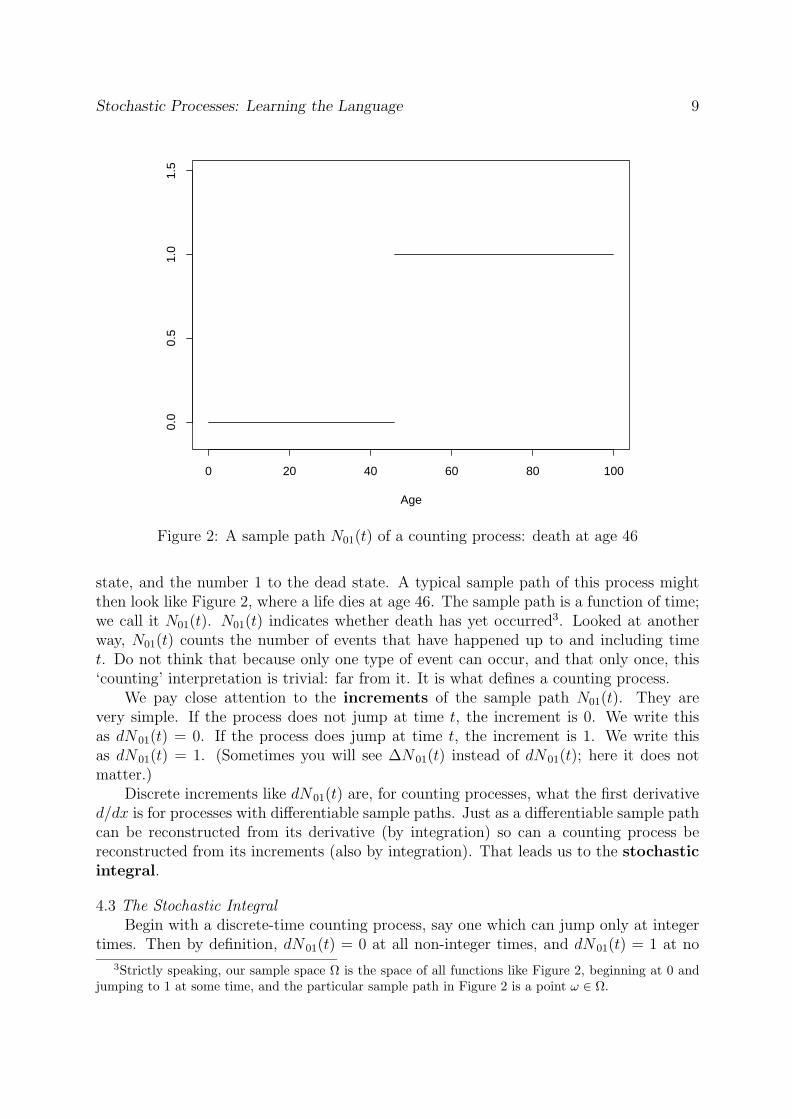
Figure 2: A sample path N01(t) of a counting process: death at age 46
state, and the number 1 to the dead state. A typical sample path of this process mightthen look like Figure 2, where a life dies at age 46. The sample path is a function of time;we call it N01(t). N01(t) indicates whether death has yet occurred3. Looked at anotherway, N01(t) counts the number of events that have happened up to and including timet. Do not think that because only one type of event can occur, and that only once, this‘counting’ interpretation is trivial: far from it. It is what defines a counting process.
We pay close attention to the increments of the sample path N01(t). They arevery simple. If the process does not jump at time t, the increment is 0. We write thisas dN01(t) = 0. If the process does jump at time t, the increment is 1. We write thisas dN01(t) = 1. (Sometimes you will see ∆N01(t) instead of dN01(t); here it does notmatter.)
Discrete increments like dN01(t) are, for counting processes, what the first derivatived/dx is for processes with differentiable sample paths. Just as a differentiable sample pathcan be reconstructed from its derivative (by integration) so can a counting process bereconstructed from its increments (also by integration). That leads us to the stochasticintegral.
4.3 The Stochastic IntegralBegin with a discrete-time counting process, say one which can jump only at integer
times. Then by definition, dN01(t) = 0 at all non-integer times, and dN01(t) = 1 at no
3Strictly speaking, our sample space Ω is the space of all functions like Figure 2, beginning at 0 andjumping to 1 at some time, and the particular sample path in Figure 2 is a point ω ∈ Ω.
Stochastic Processes: Learning the Language 10
more than one integer time. Can we reconstruct N01(t) from its increments dN01(t)? Tobe specific, can we find N01(T )? (T need not be an integer). Let J(T ) be the set of allpossible jump times up to and including T (that is, all integers ≤ T ). Then:
N01(T ) =∑
t∈J(T )
dN01(t). (1)
Suppose N01(t) is still discrete-time, but can jump at more points: for example at theend of each month. Again, define J(T ) as the set of all possible jump times up to andincluding T , and equation (1) remains valid. This works for any discrete set of possiblejump times, no matter how refined it is (years, months, days, minutes, nanoseconds . . .).What happens in the limit?(a) the counting process becomes the continuous-time version with which we started;(b) the set of possible jump times J(T ) becomes the interval (0, T ]; and(c) the sum for N01(T ) becomes an integral:
N01(T ) =∫
t∈J(T )
dN01(t) =
T∫0
dN01(t). (2)
The integral in equation (2) is a stochastic integral. Regarded as a function of T , it isa stochastic process4. This idea is very useful; it lets us write down values of assurancesand annuities.
4.4 Assurances and AnnuitiesConsider a whole life assurance paying £1 at the moment of death. What is its
present value at age x (call it X)? In Subjects A2 and 104, one way of writing this downis introduced: define Tx as the time until death of a life aged x (a random variable) andthen the present value of the assurance is X = vTx = e−δTx (in the usual notation).
We can also write this as a stochastic integral. The present value of £1 paid at timet is vt. If the life does not die at time t, the increment of the counting process N isdN01(t) = 0, and the present value of the payment is vtdN01(t) = 0. If the life does dieat time t, the increment of N is dN01(t) = 1, and the present value of the payment isvtdN01(t) = vt. Adding up (integrating) we get:
X =
∞∫0
vtdN01(t). (3)
Annuities can also be written down as stochastic integrals, with a little more notation.Consider a life annuity of 1 per annum payable continuously, and let Y be its present value.Define a stochastic process I0(t) as follows: I0(t) = 1 if the life is alive at time t, andI0(t) = 0 otherwise. This is an indicator process; it takes the value 1 or 0 dependingon whether or not a given status is fulfilled. Then:
4The stochastic integrals in this section are stochastic just because sample paths of the stochasticprocess N01(t) are involved in their definitions. Given the sample path of N01(t), these integrals areconstructed in the same way as their deterministic counterparts. The stochastic integrals needed infinancial mathematics, called Ito integrals, are a bit different.
Stochastic Processes: Learning the Language 11
Y =
∞∫0
vtI0(t)dt. (4)
Given the sample path, this is a perfectly ordinary integral, but since the sample pathis random, so is Y . Defining X(T ) and Y (T ) as the present value of payments up to timeT , we can write down the stochastic processes:
X(T ) =
T∫0
vtdN01(t) and Y (T ) =
T∫0
vtI0(t)dt. (5)
4.5 The Elements of Life Insurance MathematicsGuided by these examples, we can now write down the elements of life insurance
mathematics in terms of counting processes. This was first done surprisingly recently(Hoem & Aalen, 1978; Ramlau-Hansen 1988; Norberg 1990, 1991). We start with paymentfunctions:(a) if N = 0 at time t (the life is alive), an annuity is payable continuously at rate a0(t)
per annum; and(b) if N jumps from 0 to 1 at time t (the life dies), a sum assured of A01(t) is paid.
Noting the obvious, premiums can be treated as a negative annuity, and these definitionscan be extended to any multiple state model. Also without difficulty, discrete annuityor pure endowment payments can also be accommodated, but we leave them out forsimplicity.
The quantities a0(t) and A01(t) are functions of time, but need not be stochasticprocesses. They define payments that will be made, depending on events, but they do notrepresent the events themselves. In the case of a non-profit assurance, for example, theywill be deterministic functions of age. The payments actually made can be expressed asa rate, dL(t):
dL(t) = A01(t)dN01(t) + a0(t)I0(t)dt. (6)
This gives the net rate of payment, ‘during’ the time interval t to t + dt, depending onevents. We suppose that no payments are made after time T (T could be ∞). Thecumulative payment is then:
L =
T∫0
dL(t) =
T∫0
A01(t)dN01(t) +
T∫0
a0(t)I0(t)dt (7)
and the value of the cumulative payment at time 0, denoted V (0), is:
V (0) =
T∫0
vtdL(t) =
T∫0
vtA01(t)dN01(t) +
T∫0
vta0(t)I0(t)dt (8)
This quantity is the main target of study. Compare it with equation (5); it simply allowsfor more general payments. It is a stochastic process, as a function of T , since it now
Stochastic Processes: Learning the Language 12
represents the payments made depending on the particular life history (that is, the samplepath of N01(t)).
We also make use of the accumulated/discounted value of the payments at any times, denoted V (s):
V (s) =1
vs
T∫0
vtdL(t) =1
vs
T∫0
vtA01(t)dN01(t) +1
vs
T∫0
vta0(t)I0(t)dt. (9)
4.6 Stochastic Interest RatesAlthough we have written the discount function as vt, implicitly assuming a constant,
deterministic interest rate, this is not necessary at this stage. We could just as wellassume that the discount function was a function of time, or even a stochastic process.For simplicity, we will not pursue this, but see Norberg (1991) and Møller (1998).
4.7 Bases and Expected Present ValuesIn terms of probability models, all we have defined so far are the elements of the
sample space Ω (the sample paths N01(t)) and some related functions such as L and V (s).We have not introduced any σ-algebras, filtrations or probability measures, nor have wecarried out any probabilistic calculation, such as taking expectations. We now considerthese:(a) Our filtration is the ‘natural’ filtration generated by the process N01(t), which is easily
described. At time t, the past values N01(s) (s ≤ t) are all known, and the futurevalues N01(s) (s > t) are unknown (unless N01(t) = 1, in which case nothing morecan happen). This information is summed up by the σ-algebra Ft.To picture this filtration, cover Figure 2 with your hand, and then slowly reveal thelife history. Before age 46, all possible future life histories are hidden by your hand;the information Ft is the combination of the revealed life history and all these hiddenpossibilities.
(b) Our ‘overall’ σ-algebra F is the union of all the Ft.(c) The probability measure corresponds to the mortality basis. As is well known,
the actuary will choose a different mortality basis for different purposes, and wesuppose that nature chooses the ‘real’ mortality basis. In other words, the samplespace and the filtration do not determine the choice of probability measure; nor is thechoice of probability measure always an attempt to find nature’s ‘real’ probabilities(that is the estimation problem). This point is of even greater importance in financialmathematics, where it is often misunderstood.
All concrete calculations depend on the choice of probability measure (mortality ba-sis). We will illustrate this using expected present values. Suppose the actuary has chosena probability measure P (equivalent to life table probabilities tpx). Taking as an examplethe whole life assurance benefit, for a life aged x, say, EP [X] is:
EP
∞∫
0
vtdN01(t)
=
∞∫0
vtEP [dN01(t)] =
∞∫0
vtP[dN01(t) = 1] =
∞∫0
vttpxµx+tdt (10)

Stochastic Processes: Learning the Language 13
-¾
SS
SS
SSw
¶¶
¶¶
¶¶/
0 = able 1 = ill
2 = dead
µ01x
µ10x
µ02x µ12
x
Figure 3: An illness-death model
which should be familiar5. If the actuary chooses a different measure P ∗, say (equivalentto different life table probabilities tp
∗x), we get a different expected value:
EP ∗ [X] =
∞∫0
vttp∗xµ∗x+tdt. (11)
Expected values of annuities are also easily written:
EP [Y ] =
∞∫0
vttpxdt. (12)
4.8 More Examples of Counting ProcessesFigure 3 shows the well-known illness-death model. A precise formulation begins with
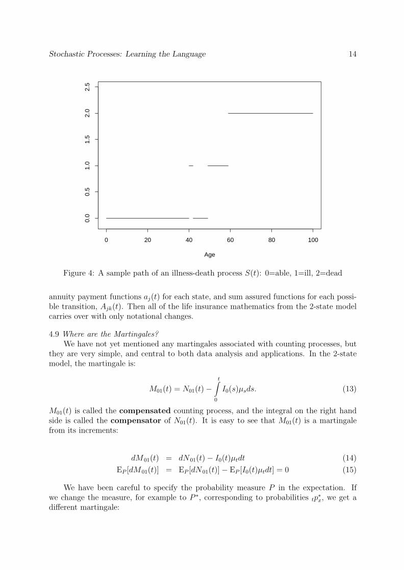
the state S(t) occupied at time t; a stochastic process.Figure 4 shows a single sample path from S(t): a life who has a short illness at age
40, recovers at age 42, then has a longer, ultimately fatal illness starting at age 49. Inthe 2-state mortality model, the stochastic process S(t), representing the state occupied,coincided with the counting process N01(t) representing the number of events6: here it isnot so. In fact we can define 4 counting processes, one for each transition, for example:
N01(t) = No. of transitions able to ill
N02(t) = No. of transitions able to dead
N10(t) = No. of transitions ill to able
N12(t) = No. of transitions ill to dead
or, regarding them as one object, we have a multivariate counting process with 4 com-ponents. We can also define stochastic processes indicating presence in each state, Ij(t),
5The last step in equation (10) follows because the event dN01(t) = 1 is just the event ‘survives tojust before age x + t, then dies in the next instant’, which has the probability tpxµx+tdt.
6We did not introduce S(t) for the 2-state model: we do so now, it is the same as N01(t).
Stochastic Processes: Learning the Language 14
Age
0 20 40 60 80 100
0.0
0.5
1.0
1.5
2.0
2.5
Figure 4: A sample path of an illness-death process S(t): 0=able, 1=ill, 2=dead
annuity payment functions aj(t) for each state, and sum assured functions for each possi-ble transition, Ajk(t). Then all of the life insurance mathematics from the 2-state modelcarries over with only notational changes.
4.9 Where are the Martingales?We have not yet mentioned any martingales associated with counting processes, but
they are very simple, and central to both data analysis and applications. In the 2-statemodel, the martingale is:
M01(t) = N01(t)−t∫
0
I0(s)µsds. (13)
M01(t) is called the compensated counting process, and the integral on the right handside is called the compensator of N01(t). It is easy to see that M01(t) is a martingalefrom its increments:
dM01(t) = dN01(t)− I0(t)µtdt (14)
EP [dM01(t)] = EP [dN01(t)]− EP [I0(t)µtdt] = 0 (15)
We have been careful to specify the probability measure P in the expectation. Ifwe change the measure, for example to P ∗, corresponding to probabilities tp
∗x, we get a
different martingale:

Stochastic Processes: Learning the Language 15
M∗01(t) = N01(t)−
t∫0
I0(s)µ∗sds (16)
and EP ∗ [dM∗01(t)] = 0. Alternatively, given a force of mortality µ∗t , we can find a probabil-
ity measure P ∗ such that M∗01(t) is a P ∗-martingale; P ∗ is simply given by the probabilities
tp∗x = exp(− ∫ t
0 µ∗sds). This is true of any (well-behaved) force of mortality, not just na-ture’s chosen ‘true’ force of mortality7.
An idea of the usefulness of M01(t) can be gained from equation (13). If we con-sider an age interval short enough that a constant transition intensity µ is a reasonableapproximation, this becomes:
M01(t) = N01(t)− µ
t∫0
I0(s)ds. (17)
But the two random quantities on the right are just the number of deaths N01(t), and thetotal time spent at risk
∫ t0 I0(s)ds, better known as the central exposed to risk. All the
properties of the maximum likelihood estimate of µ, based on these two statistics (summedover many independent lives) are consequences of the fact that M01(t) is a martingale (seeMacdonald (1996a, 1996b)).
For more complicated models, we get a set of martingales, one for each possibletransition (from state j to state k) of the form:
Mjk(t) = Njk(t)−t∫
0
Ij(s)µjks ds (18)
which have all the same properties.
4.10 Prospective and Retrospective ReservesWe now return to equation (9): V (s) = v−s
∫ T0 vtdL(t). Recall that the premium is
part of the payment function a0(t); setting the premium according to the equivalenceprinciple simply means setting EP [V (0)] = 0 and solving for a0(t), where P is theprobability measure corresponding to the premium basis.
For convenience, we will use the same basis (measure) for premiums and reserves, asis common in other European countries.
Reserves follow when we consider the evolution of the value function V over time, asinformation emerges. We start from the conditional expectation; for s < T :
EP [V (s)|Fs] = EP
1
vs
T∫0
vtdL(t)
∣∣∣∣∣ Fs
(19)
7This is exactly analogous to the ‘equivalent martingale measure’ of financial mathematics, in whichwe are given the drift of a geometric Brownian motion (coincidentally, also often denoted µt) and thenfind a probability measure under which the discounted process is a martingale.

Stochastic Processes: Learning the Language 16
= EP
1
vs
s∫0
vtdL(t)
∣∣∣∣∣ Fs
+ EP
1
vs
T∫s
vtdL(t)
∣∣∣∣∣ Fs
(20)
The second term on the right is the prospective reserve at time s. If the informationFs is the complete life history up to time s, it is the same as the usual prospectivereserve. However, this definition is more general; for example, under a joint-life second-death assurance, the first death might not be reported, so that Fs represents incompleteinformation. Also, it does not depend on the probabilistic nature of the process generatingthe life history; it is not necessary to suppose that the process is Markov, for example.If the process is Markov (as we often suppose) then conditioning on Fs simply meansconditioning on the state occupied at time s, which is very convenient in practice.
The first term on the right is minus the retrospective reserve. This definition of theretrospective reserve is new (Norberg, 1991) and is not equivalent to ‘classical’ definitions.This is a striking achievement of the stochastic process approach: for convenience we alsolist some of the notions of retrospective reserve that have preceded it:(a) The ‘classical’ retrospective reserve (for example, Neill (1977)) depends on a deter-
ministic cohort of lives, who share out a fund among survivors at the end of theterm. However, this just exposes the weaknesses of the deterministic model: givena whole number of lives at outset, lx say, the number of survivors some time later,lxtpx is usually not an integer. Viewed prospectively this can be excused as being aconvenient way of thinking about expected values, but viewed retrospectively thereis no such excuse.
(b) Hoem (1969) allowed both the number of survivors, and the fund shared amongsurvivors, to be random, and showed that the classical retrospective reserve wasobtained in the limit, as the number of lives increased to infinity.
(c) Perhaps surprisingly, the ‘classical’ notion of retrospective reserve does not lead to aunique specification of what the reserve should be in each state of a general Markovmodel, leading to several alternative definitions (Hoem, 1988; Wolthius & Hoem, 1990;Wolthius, 1992) in which the retrospective and prospective reserves in the initial statewere equated by definition.
(d) Finally, Norberg (1991) pointed out that the ‘classical’ retrospective reserve is “. . .rather a retrospective formula for the prospective reserve . . .”, and introduced the def-inition in equation (20). This is properly defined for individual lives, and depends onknown information Fs. If Fs is the complete life history, the conditional expectationdisappears and:
Retrospective reserve =−1
vs
s∫0
vtdL(t) (21)
which is more akin to an asset share on an individual policy basis. If Fs representscoarser information, for example aggregate data in respect of a cohort of policies, theretrospective reserve is akin to an asset share with pooling of mortality costs.
We have spent some time on retrospective reserves, because it is an example of thegreater clarity obtained from a careful mathematical formulation of the process beingmodelled, in this case the life history.
Stochastic Processes: Learning the Language 17
4.11 Differential EquationsThe chief computational tools associated with multiple-state models are ordinary
differential equations (ODEs). We mention three useful systems of ODEs:(a) The Kolmogorov forward equations can be found in any textbook on Markov
processes (for example, Kulkarni (1995)) and have been in the actuarial syllabus forsome time. They allow us to calculate transition probabilities in a Markov process,given the transition intensities, which is exactly what we need since transition inten-sities are the quantities most easily estimated from data. We give just one example,the simplest of all from the 2-state model:
∂
∂ttpx = −tpxµx+t. (22)
(b) Theile’s equation governs the development of the prospective reserve. For example,if tV x is the reserve under a whole life assurance for £1, Theile’s equation is:
d
dttV x = δtV x + P x − (1− tV x)µx+t (23)
which has a very intuitive interpretation. In fact, it is the continuous-time equivalentof the recursive formula for reserves well-known to British actuaries. It was extendedto any Markov model by Hoem (1969).
(c) Norberg (1995b) extended Theile’s equations for prospective policy values (that is,first moments of present values) to second and higher moments. We do not showthese equations, as that would need too much new notation, but we note that theywere obtained from the properties of counting process martingales.
Most systems of ODEs do not admit closed-form solutions, and have to be solved nu-merically, but many methods of solution are quite simple8, and well within the capabilityof a modern PC. So, while closed-form solutions are nice, they are not too important,and it is better to seek ODEs that are relevant to the problem, rather than explicitlysoluble. We would remind actuaries of a venerable example of a numerical solution to anintractable ODE, namely the life table.
4.12 Advantages of the Counting Process Approach(a) First and foremost, counting processes represent complete life histories. In practice,
not all this information might be available or useable, but it is best to start with amodel that represents the underlying process, and then to make whatever approxi-mations might be needed to meet the circumstances (for example, data grouped intoyears).
(b) The mathematics of counting processes and multiple-state models is easily introducedin terms of the 2-state mortality model, but carries over to any more complicatedmodel, thus solving problems that defeat life-table methods. This is increasinglyimportant in practice, as new insurances are introduced.
(c) Completely new results have been obtained, such as an operational definition of ret-rospective reserves, and Norberg’s differential equations.
8Numerical solution of ODEs is one of the most basic tasks in numerical analysis.
Stochastic Processes: Learning the Language 18
(d) The tools we use are exactly those that are essential in modern financial mathematics,in particular stochastic integrals and conditional expectations. For a remarkable syn-thesis of these two fields, see Møller (1998). An alternative approach, in which ratesof return as well as lifetimes are modelled by Markov processes, has been developed(Norberg, 1995b) extending greatly the scope of the material discussed here.
(e) We have not discussed data analysis, but mortality studies are increasingly turningtowards counting process tools, for exactly the same reason as in (a). It will often behelpful for actuaries at least to understand the language.
5. Finance
5.1 IntroductionIn this section we are going to illustrate how stochastic processes can be used to price
financial derivatives.A financial derivative is a contract which derives its value from some underlying
security. For example, a European call option on a share gives the holder the right, butnot the obligation, to buy the share at the exercise date T at the strike price of K. If theshare price at time T , ST , is less than K then the option will not be exercised and it willexpire without any value. If ST is greater than K then the holder will exercise the optionand a profit of ST −K will be made. The profit at T is, therefore, maxST −K, 0.
5.2 Models of Asset PricesMuch of financial mathematics must be based on explicit models of asset prices,
and the results we get depend on the models we decide to use. In this section we willlook at two models for share prices: a simple binomial model which will bring out themain points; and geometric Brownian motion. Throughout we make the following generalassumptions9.(a) We will use St to represent the price of a non-dividend-paying stock at time t (t =
0, 1, 2, . . .). For t > 0, St is random.(b) Besides the stock we can also invest in a bond or a cash account which has value Bt
at time t per unit invested at time 0. This account is assumed to be risk free and wewill assume that it earns interest at the constant risk-free continuously compoundingrate of r per annum. Thus Bt = exp(rt). (In discrete time, risk free means that weknow at time t − 1 what the value of the risk-free investment will be at time t. Inthis more simple case, the value of the risk-free investment at any time t is known attime 0.)
(c) At any point in time we can hold arbitrarily large amounts (positive or negative) ofstock or cash.
5.3 The No-Arbitrage PrincipleBefore we progress it is necessary to discuss arbitrage.
9These assumptions can be relaxed considerably with more work.
Stochastic Processes: Learning the Language 19
Suppose that we have a set of assets in which we can invest (with holdings which canbe positive or negative). Consider a particular portfolio which starts off with value zeroat time 0 (so we have some positive holdings and some negative). With this portfolio,it is known that there is some time T in the future when its value will be non-negativewith certainty and strictly positive with probability greater than zero. This is called anarbitrage opportunity. To exploit it we could multiply up all amounts by one thousandor one million and make huge profits without any cost or risk.
In financial mathematics and derivative pricing we make the fundamental assumptionthat arbitrage opportunities like this do not exist (or at least that if they do exist, theydisappear too quickly to be exploited).
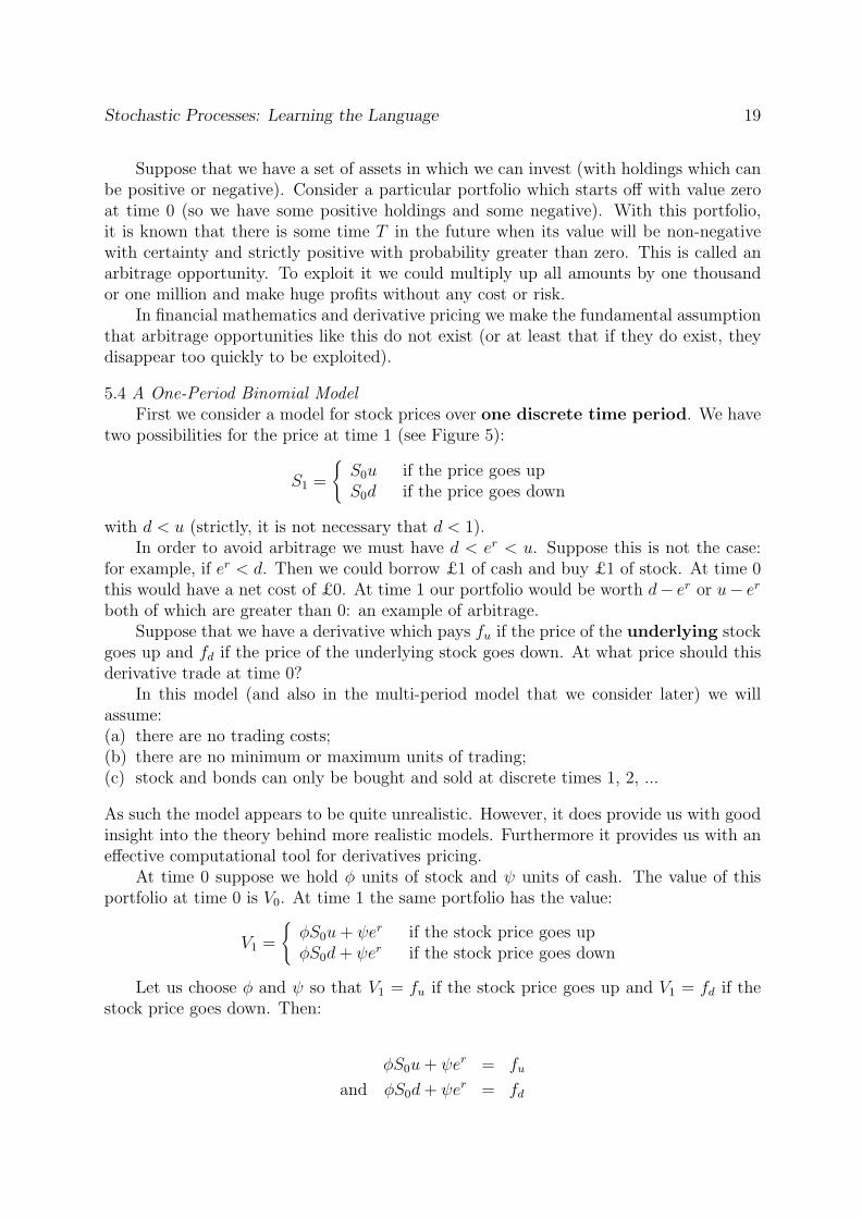
5.4 A One-Period Binomial ModelFirst we consider a model for stock prices over one discrete time period. We have
two possibilities for the price at time 1 (see Figure 5):
S1 =
S0u if the price goes upS0d if the price goes down
with d < u (strictly, it is not necessary that d < 1).In order to avoid arbitrage we must have d < er < u. Suppose this is not the case:
for example, if er < d. Then we could borrow £1 of cash and buy £1 of stock. At time 0this would have a net cost of £0. At time 1 our portfolio would be worth d− er or u− er
both of which are greater than 0: an example of arbitrage.Suppose that we have a derivative which pays fu if the price of the underlying stock
goes up and fd if the price of the underlying stock goes down. At what price should thisderivative trade at time 0?
In this model (and also in the multi-period model that we consider later) we willassume:(a) there are no trading costs;(b) there are no minimum or maximum units of trading;(c) stock and bonds can only be bought and sold at discrete times 1, 2, ...
As such the model appears to be quite unrealistic. However, it does provide us with goodinsight into the theory behind more realistic models. Furthermore it provides us with aneffective computational tool for derivatives pricing.
At time 0 suppose we hold φ units of stock and ψ units of cash. The value of thisportfolio at time 0 is V0. At time 1 the same portfolio has the value:
V1 =
φS0u + ψer if the stock price goes upφS0d + ψer if the stock price goes down
Let us choose φ and ψ so that V1 = fu if the stock price goes up and V1 = fd if thestock price goes down. Then:
φS0u + ψer = fu
and φS0d + ψer = fd

Stochastic Processes: Learning the Language 20
©©©©©©*
HHHHHHj
uu
uS0
S0u
S0d
Figure 5: One-period binomial model for stock prices
Thus we have two linear equations in two unknowns, φ and ψ. We solve this system ofequations and find that:
φ =fu − fd
S0(u− d)
ψ = e−r(fu − φS0u)
= e−r
(fu −
(fu − fd)u
u− d
)
= e−r
(fdu− fud
u− d
)
⇒ V0 = φS0 + ψ
=(fu − fd)
u− d+ e−r (fdu− fud)
u− d
= fu
(1− de−r
u− d
)+ fd
(−1 + ue−r
u− d
)
= e−r (qfu + (1− q)fd)
where q =er − d
u− d
1− q =u− er
u− d= 1− er − d
u− d
Note that the no-arbitrage condition d < er < u ensures that 0 < q < 1.If we denote the payoff of the derivative at t = 1 by the random variable f(S1), we
can write:
V0 = e−rEQ(f(S1))
where Q is a probability measure which gives probability q to an upward move in pricesand 1 − q to a downward move. We can see that q depends only upon u, d and r andnot upon the potential derivative prices. In particular, Q does not depend on the type ofderivative; it is the same for all derivatives on the same stock.
Stochastic Processes: Learning the Language 21
The portfolio (φ, ψ) is called a replicating portfolio because it replicates, precisely,the payoff at time 1 on the derivative without any risk. It is also a simple example of ahedging strategy: that is, an investment strategy which reduces the amount of risk carriedby the issuer of the contract. In this respect not all hedging strategies are replicatingstrategies.
Up until now we have not mentioned the real-world probabilities of up and downmoves in prices. Let these be p and 1−p where 0 < p < 1, defining a probability measureP .
Other than by total coincidence, p will not be equal to q.Let us consider the expected stock price at time 1. Under P this is:
S0(pu + (1− p)d) = EP (S1)
and under Q it is:
EQ(S1) = S0(qu + (1− q)d) = S0
(u(er − d)
u− d+
d(u− er)
u− d
)= S0e
r.
Under Q we see that the expected return on the risky stock is the same as that ona risk-free investment in cash. In other words under the probability measure Q investorsare neutral with regard to risk: they require no additional returns for taking on more risk.This is why Q is sometimes referred to as a risk-neutral probability measure.
Under the real-world measure P the expected return on the stock will not normallybe equal to the return on risk-free cash. Under normal circumstances investors demandhigher expected returns in return for accepting the risk in the stock price. Thus we wouldnormally find that p > q. However, this makes no difference to our analysis.
5.5 Comparison of Actuarial and Financial Economic ApproachesThe actuarial approach to the pricing of this contract would give:
V a0 = e−δEP [f(S1)] = e−δ(pfu + (1− p)fd)
where δ is the actuarial, risk-discount rate. Compare this with the price calculated usingthe principles of financial economics above:
V0 = e−rEQ(f(S1)) = e−r(qfu + (1− q)fd).
If forwards are trading at V a0 , where V a
0 > V0, then we can sell one derivative at theactuarial price, and use an amount V0 to set up the replicating portfolio (φ, ψ) at time0. The replicating portfolio ensures that we have the right amount of money at t = 1 topay off the holder of the derivative contract. The difference between V a
0 and V0 is thenguaranteed profit with no risk.
Similarly if V a0 < V0 we can also make arbitrage profits.
(In fact neither of these situations could persist for any length of time because demandfor such contracts trading at V a
0 would push the price back towards V0 very quickly. This isa fundamental principle of financial economics: that is, prices should not admit arbitrage
Stochastic Processes: Learning the Language 22
opportunities. If they did exist then the market would spot any opportunities very quicklyand the resulting excess supply or demand would remove the arbitrage opportunity beforeany substantial profits could be made. In other words, arbitrage opportunities mightexist for very short periods of time in practice, while the market is free from arbitragefor the great majority of time and certainly at any points in time where large financialtransactions are concerned. Of course, we would have no problem in buying such acontract if we were to offer a price of V a
0 to the seller if this was greater than V0 but wewould not be able to sell at that price. Similarly we could easily sell such a contract ifV a
0 < V0 but not buy at that price. In both cases we would be left in a position where wewould have to maintain a risky portfolio in order to give ourselves a chance of a profit,since hedging would result in a guaranteed loss.)
For V a0 to make reasonable sense, then, we must set δ in such a way that V a
0 equalsV0. In other words, the subjective choice of δ in actuarial work equates to the objectiveselection of the risk-neutral probability measure Q. Choosing δ to equate V a
0 and V0
is not what happens in practice and, although δ is set with regard to the level of riskunder the derivative contract, the subjective element in this choice means that there isno guarantee that V a
0 will equal V0. In general, therefore, the actuarial approach, onits own, is not appropriate for use in derivative pricing. Where models are generalisedand assumptions weakened to such an extent that it is not possible to construct hedgingstrategies which replicate derivative payoffs then there is a role for a combination of thefinancial economic and actuarial approaches. However, this is beyond the scope of thispaper.
5.6 Binomial LatticesNow let us look at how we might price a derivative contract in a multiperiod model
with n time periods. Let f(x) be the payoff on the derivative if the share has a price of x atthe expiry date n. For example, for a European call option we have f(x) = maxx−K, 0,where K is the strike price.
Suppose now that over each time period the share price can rise by a factor of u orfall by a factor of d = 1/u: that is, for all t, St+1 is equal to Stu or Std. This meansthat the effect of successive ‘up and down’ moves is the same as successive ‘down and up’moves. Furthermore the risk-free rate of interest is constant and equal to r, with, still,d < er < u. Then we have:
St = S0uNtdt−Nt
where Nt is the number of up-steps10 between time 0 and time t. This means that wehave n+1 possible states at time n. We can see that the value of the stock price at time tdepends only upon the number of up and down steps and not on the order in which theyoccurred. Because of this property the model is called a recombining binomial treeor a binomial lattice (see Figure 6).
The sample space for this model, Ω, is the set of all sample paths from time 0 to timen. This is widely known as the random walk model.There are 2n such sample paths sincethere are two pssible outcomes in each time period. The information F is the σ-algebra
10In this sense, Nt can also be regarded as a discrete-time counting process; see Section 4.

Stochastic Processes: Learning the Language 23
uS0©©©©©©*
HHHHHHj
u S0u©©©©©©*
HHHHHHj
u S0d©©©©©©*
HHHHHHj
u S0u2©©©©©©*
HHHHHHj
u S0ud©©©©©©*
HHHHHHj
u S0d2©©©©©©*
HHHHHHj
u S0u3©©©©©©*
HHHHHHj
u S0u2d©©©©©©*
HHHHHHj
u S0ud2©©©©©©*
HHHHHHj
u S0d3©©©©©©*
HHHHHHj
u S0u4
u S0u3d
u S0u2d2
u S0ud3
u S0d4
Figure 6: Recombining binomial tree or binomial lattice
generated by all sample paths from time 0 to n while the filtrations Ft are generated byall sample paths up to time t. (Given the sample space Ω, each sample path up to time tis equivalent to 2n−t elements of the sample space, each element being the same over theperiod 0 to t. Nt and St are random variables which are functions of the sample space.)
Under this model all periods have the same probability of an up step and steps ineach time period are independent of one another. Thus the number of up steps up totime t, Nt, has under Q a binomial distribution with parameters t and q. Furthermore,for 0 < t < n, Nt is independent of Nn−Nt and Nn−Nt has a binomial distribution withparameters n− t and q.
Let us extend our notation a little bit. Let Vt(j) be the fair value of the derivativeat time t given Nt = j for j = 0, . . . , t. Also let Vn(j) = f (S0u
jdn−j). Finally we writeVt = Vt(Nt) to be the random value at some future time t.
In order for us to calculate the value at time 0, V0(0), we must work backwards oneperiod at a time from time n making use of the one-period binomial model as we go.
First let us consider the time period n − 1 to n. Suppose that Nn−1 = j. Then, byanalogy with the one-period model we have:
Stochastic Processes: Learning the Language 24
Vn−1(j) = e−r [qVn(j + 1) + (1− q)Vn(j)]
= e−rEQ [Vn | Fn−1]
= e−rEQ [f(Sn) | Nn−1 = j]
= e−rEQ [f(Sn) | Fn−1]
where q =er − d
u− d.
Equivalently we can write this as Vn−1 = e−rEQ[f(Sn) | Fn−1].As we work backwards we have:
Vt−1 = e−rEQ[Vt | Ft−1]
= e−rEQ
[e−rEQ (Vt+1 | Ft) | Ft−1
]= e−2rEQ [Vt+1 | Ft−1] (using the Tower Law)...
......
= e−(n−t+1)rEQ [Vn | Ft−1]
= e−(n−t+1)rEQ [f(Sn) | Ft−1] .
Finally we get to:
V0 = e−nrEQ [f(Sn) | F0] = e−nrEQ [f(Sn) | S0] .
The price at time t of the path-dependent derivative is thus:
Vt = e−r(n−t)EQ
[f
(Stu
Nn−Ntd(n−t)−(Nn−Nt))| Nt
]
= e−r(n−t)n−t∑k=0
f(Stu
kdn−t−k) (n− t)!
k!(n− t− k)!qk(1− q)n−t−k.
We have noted before that EQ(S1) = S0er giving rise to the use of the name risk-
neutral measure for Q. Similarly in the n-period model we have (putting f(s) = s):
EQ[St|F0] = S0ert.
So the use of the expression risk-neutral measure for Q is still valid. Alternatively wecan write:
EQ
[e−rT ST | Ft
]= e−rtSt.
In other words, the discounted asset value process Dt = e−rtSt is a martingale under Q.This gives rise to another name for Q: equivalent martingale measure.
Stochastic Processes: Learning the Language 25
In fact we normally use this result the other way round, as we will see in the nextsection. That is, the first thing we do is to find the equivalent martingale measure Q, andthen use it immediately to price derivatives.
5.7 A Continuous Time ModelLet us now work in continuous time. Let St be the price of the non-dividend-paying
share for 0 ≤ t ≤ T . Suppose that a derivative pays f(s) at time T if the share price attime T is equal to s.
The particular model we are going to look at for St is called geometric Brownianmotion: that is, St = S0 exp[(µ− 1
2σ2)t + σZt] where Zt is a standard Brownian motion
under the real-world measure P . (For the properties of Brownian motion see AppendixA.) This means that St has a log-normal distribution with mean S0 exp(µt) and varianceexp(2µt). [exp(σ2t)− 1]. By application of Ito’s lemma (see Appendix B) we can writedown the stochastic differential equation (SDE) for St as follows:
dSt = µStdt + σStdZt.
By analogy with the binomial model there is another probability measure Q (therisk-neutral measure or equivalent martingale measure) under which:(a) e−rtSt is a martingale
(b) St can be written as the geometric Brownian motion S0 exp[(
r − 12σ2
)t + σZt
]where
Z(t) is a standard Brownian motion under Q
By continuing the analogy with the binomial model (for example, see Baxter & Rennie(1996)) we can also say that the value at time t of the derivative is:
Vt = e−r(T−t)EQ [f(ST ) | Ft] = e−r(T−t)EQ [f(ST ) | St] .
With a bit more work we can also see that, under this model, if we invest Vt in theright way (that is, with a suitable hedging strategy), then we can replicate the payoff atT without the need for extra cash.
Suppose that we consider a European call option, so that f(s) = maxs−K, 0. Thenwe can exploit a well known property of the log-normal distribution to get the celebratedBlack-Scholes formula:
Vt = StΦ(d1)−Ke−r(T−t)Φ(d2)
where d1 =log St
K+
(r + 1
2σ2
)(T − t)
σ√
T − t
and d2 = d1 − σ√
T − t.
A more detailed development of pricing and hedging of derivatives in continuous timecan be found in Baxter & Rennie (1996).

Stochastic Processes: Learning the Language 26
5.8 Guaranteed annuity contracts: a cautionary taleA more complex example, where stochastic processes (randomness is perhaps more
important than the time element) must be used is the problem of guaranteed annuitycontracts. We can state the problem quite simply. A contract of this type will convert thepolicyholder’s fund at maturity, F (T ), into an annuity at the lower of the market rate,a(T ) (which takes into account current market rates of interest and mortality rates), and aminimum guarantee, amin. The value at maturity is maxF (T )/a(T ), F (T )/amin. Moresimply we can write this as maxX,Y where X = F (T )/a(T ) and Y = F (T )/amin aredependent random variables. Ignoring the time value of this contract the expected valueof this contract is E[maxX,Y ]. This is greater than maxE[X], E[Y ] by a simpleapplication of Jensen’s inequality. By implication this in turn exceeds E[X] and E[Y ].Twenty years ago actuaries took E[X] as the value of this contract assuming that interestrates would never fall far enough for the guarantee to lock in. Now that interest rateshave fallen, many actuaries are taking the value as maxE[X], E[Y ]. It is important tounderstand the distinction between this and E[ maxX,Y ]. When you see this then youwill see why an understanding of the underlying randomness is essential to the accuratepricing of this type of contract.
6. Risk Theory
6.1 IntroductionIn this section we show how stochastic processes can be used to gain insight into the
pricing of general insurance policies. In particular, we will make use of the notion of amartingale, Brownian motion and also the optional stopping theorem.
Suppose we have a general insurance risk, for example comprehensive insurance fora fleet of cars or professional indemnity insurance for a software supplier, for which coveris required on an annual basis. We want to answer the question: “In an ideal world,how should we calculate the annual premium for this cover?” Let us denote by Pn thepremium to be charged for cover in year n, where the coming year is year 1.
The starting point is to consider the claims which will arise each year. Since theaggregate amount of claims is uncertain, we model these amounts as random variables.Let Sn be a random variable denoting the aggregate claims arising from the risk in year n.We might also take into consideration, particularly for a large risk, the amount of capitalwith which we are prepared to back this risk. We denote this initial capital, or ‘initialsurplus’, U . In practice, we would also take into consideration many other factors, forexample, expenses and the premium rates charged by our competitors. However, to keepthings simple, we will ignore these other factors.
Throughout this section we will assume that the random variables Sn∞n=1 are inde-pendent of each other, but we will not assume they are identically distributed. To be ableto calculate Pn we need to be able to calculate, or at least estimate, the distribution ofSn. If we have information about the distributions of claim numbers and claim amountsin year n, we may be able to use Panjer’s celebrated recursion formula to calculate thedistribution of Sn. See, for example, Klugman et al (1997). In some circumstances, forexample when Sn is the sum of a large number of independent claim amounts, it may be

Stochastic Processes: Learning the Language 27
reasonable to assume that Sn has, approximately, a normal distribution. In what followswe will occasionally make the following assumption:
Sn ∼ N(µn, σ2n) (24)
for some parameters µn and σn.
6.2 The Standard Deviation PrincipleSuppose we decide that each year Pn should be set at a level such that the probability
that aggregate claims exceed the premium in that year should be suitably small, say 1−p.Formally, this criterion can be expressed as follows:
P[Sn < Pn] = p. (25)
Making the additional assumption that Sn is normally distributed, that is, assumption(24), it is easy to see that:
Pn = µn + γpσn (26)
where γp is such that:
Φ(γp) = p
and Φ(.) is the cumulative distribution function of the N(0, 1) distribution.Formula (26) says that in year n, Pn should be calculated as the mean of the aggregate
claims for that year plus a loading proportional to the standard deviation of the aggregateclaims. Notice that the proportionality factor, γp, does not depend on n. In the actuarialliterature, formula (26) is known as the standard deviation principle for the calculationof premiums, and γp is referred to as the loading factor. See Goovaerts, De Vylder, &Haezendonck (1984).
6.3 Utility Functions and the Variance PrincipleNow suppose that our attitude to money is summarised by a utility function, u(x).
Intuitively, u(x) is a real-valued function which expresses ‘how much we like an amountof money x’. Mathematically, we require the following two conditions to hold:
d
dxu(x) > 0 and
d2
dx2u(x) < 0.
The first of these conditions says that “we always prefer more money”. The secondcondition says that “an extra pound is worth less, the wealthier we are”. See Bowers etal. (1997) for more details.
We can use this utility function to calculate Pn from the following formula:
u(W ) = E[u(W + Pn − Sn)] (27)
where W is our wealth at the start of the n-th year. The rationale behind this formulais as follows: if we do not insure this risk, the utility of our wealth is u(W ); if we do
Stochastic Processes: Learning the Language 28
insure the risk, our expected utility of wealth at the end of the year is E[u(W +Pn−Sn)].Formula (27) says that for a premium of Pn we are indifferent between insuring the riskand not insuring it. In this sense the premium Pn is ‘fair’. See, for example, Bowers etal. (1997) for details.
Now assume that u(x) is an exponential utility function with parameter α > 0,so that:
u(x) = 1− e−αx. (28)
Using (28) in (27) and solving for Pn, we have:
Pn = α−1 log (MSn(α)) (29)
where the notation MZ(.) denotes the moment generating function of a random variableZ, so that MZ(α) = E[eαZ ]. Notice that in this special case Pn does not depend on W ,our wealth at the start of the n-th year.
Finally, let us assume that Sn has a normal distribution, as in (24). Then:
MSn(α) = expµnα +1
2α2σ2
n
and so (29) becomes:
Pn = µn +1
2ασ2
n. (30)
Thus, Pn is calculated according to the variance principle.
6.4 Multi-period Analysis — Discrete TimeFormulae (26) and (30) provide two alternative ways of calculating Pn in an ideal
world. They have some features in common:(a) in each case Pn is the sum of the expected value of Sn and a positive loading; and(b) in each case we arrived at a formula for Pn by considering the n-th year in isolation
from any other years.
A major difference in the development so far is that for (26) the loading factor γp has anintuitive meaning, whereas in (30), or (29), the parameter α is not so easily understoodor quantified. To fill in this gap, we need to consider our surplus at the end of each yearin the future.
Let Un denote the surplus at the end of the n-th year, so that:
Un = U +n∑
k=1
(Pk − Sk)
for n = 1, 2, 3, . . ., with U0 defined to be U . Now define:
ψ(U) = P[Un ≤ 0 for some n, n = 1, 2, 3, . . .]
Stochastic Processes: Learning the Language 29
to be the probability that at some time in the future we will need more capital to backthis risk, that is, in more emotive language, the probability of ultimate ruin in discretetime for our surplus process. Let us assume that Pn is calculated using (29).
Consider the process Yn∞n=0, where Yn = exp−αUn for n = 0, 1, 2, ... . ThenYn∞n=0 is a martingale with respect to Sn∞n=1. To prove this, note that:
Un+1 = Un + Pn+1 − Sn+1
implies that:
E [Yn+1|S1, . . . , Sn]
= E [exp−α (Un + Pn+1 − Sn+1) |S1, . . . , Sn]= E [exp−α(Pn+1 − Sn+1)|S1, . . . , Sn] exp−αUn.
Since Sn∞n=1 is a sequence of independent random variables it follows that:
E [exp−α(Pn+1 − Sn+1)|S1, . . . , Sn]
= E[exp−α(Pn+1 − Sn+1)]= exp−αPn+1E [expαSn+1]= 1
where the final step follows from (29). Hence:
E [Yn+1|S1, ..., Sn] = exp−αUn = Yn,
and so the proof is complete.We can now use this fact to find a bound for ψ(U). To do so, let us introduce the
positive constant b > U , and define the stopping time T by:
T = min(n: Un ≤ 0 or Un ≥ b) :
Thus, the process stops when the first of two events occurs: (i) ruin; or, (ii) the surplusreaches at least level b. The optional stopping theorem tells us that:
E [exp−αUT] = exp−αU.
Let pb denote the probability that ruin occurs without the surplus ever having beenat level b or above. Then, conditioning on the two events described above:
E [exp−αUT] = E [exp−αUT|UT ≤ 0] pb
+E [exp−αUT|UT ≥ b] (1− pb) (31)
= exp−αU.
Stochastic Processes: Learning the Language 30
Now let b →∞. Then pb → ψ(u), the first expectation on the right hand side of (31)is at least 1 since it is the moment generating function of the deficit at ruin, evaluated atα, and the second expectation goes to 0 since it is bounded above by exp−αb. Thus:
exp−αU = ψ(U)E [exp−αUT|UT ≤ 0]
giving:
ψ(U) =exp−αU
E [exp−αUT|UT ≤ 0]≤ exp−αU. (32)
This gives us a simple bound on the probability of ultimate ruin. It also suggests anappropriate value for the parameter α in formula (29). For example, if the initial surplusis 10, and we require that the probability of ultimate ruin is to be no more than 1%, thenwe require α such that exp−10α = 0.01, giving α = 0.461.
Let us consider the special case when Sn∞n=1 is a sequence of independent and iden-tically distributed random variables, each distributed as compound Poisson with Poissonparameter λ. Then Pn is independent of n, say Pn = P , and:
P = α−1 log E [expαSn]= α−1 log [expλ (MX(α)− 1)]
where MX(.) is the moment generating function of the distribution of a single claimamount, giving:
λ + Pα = λMX(α). (33)
This is the equation for the adjustment coefficient for this model (see, for exam-ple, Gerber (1979)). Thus, in this particular case, the parameter α is the adjustmentcoefficient, and equation (32) is simply Lundberg’s inequality.
6.5 Multi-period Analysis — Continuous TimeFormula (32) shows that when the annual premium is calculated according to formula
(29), the probability of ultimate ruin in discrete time for our surplus process is boundedabove by exp−αU. If, in addition, the distribution of aggregate claims each year is nor-mal (assumption (24)) then formula (29) implies that the premium loading is proportionalto the variance of the aggregate claims.
We can gain a little more insight, particularly into formula (32), by moving froma discrete time model to a continuous time model. In this section we assume that theaggregate claims in the time interval [0, t] are a random variable µt + σB(t), where thestochastic process B(t)t≥0 is standard Brownian motion (see Appendix A). This meansthat in any year, the aggregate claims are distributed as N(µ, σ2), and are independent ofthe claims in any other year. This is the continuous time version of assumption (24), butnote that we are now assuming that the mean and variance of the annual aggregate claimsdo not change over time. Brownian motion has stationary and independent incrementsso for any 0 ≤ s < t:
Stochastic Processes: Learning the Language 31
B(t)−B(s) ∼ N((t− s)µ, (t− s)σ2
). (34)
We assume that premiums are received continuously at constant rate P per annum,where:
P = µ +1
2ασ2 (35)
which is equivalent to formula (30). The surplus at time t is denoted U(t), where:
U(t) = U + Pt− (µt + σB(t)). (36)
Now let:
ψc(U) = P[U(t) ≤ 0 for some t, t > 0]
so that ψc(U) is the probability of ultimate ruin in continuous time for our surplus process.We will apply the martingale argument of the previous subsection to find ψc(U). Firstnote that:
E[exp−α((P − µ)t− σB(t))] = 1. (37)
This follows from formulae (34) and (35) and the formula for the moment generatingfunction of the normal distribution.
Next, let Y (t) = E[exp−αU(t)]. Then the process Y (t)t≥0 is a martingale withrespect to11 B(t)t≥0. (Since U(t)t≥0 is a continuous time stochastic process, Y (t)t≥0
is a martingale in continuous time.) This follows since for t > s:
E[Y (t)|B(u), 0 ≤ u ≤ s]
= E[exp−αU(t)|B(u), 0 ≤ u ≤ s]
= E[exp−α(U(t)− U(s)) exp−αU(s)|B(u), 0 ≤ u ≤ s].
Hence:
E[Y (t)|B(u), 0 ≤ u ≤ s]
= E[exp−α(U(t)− U(s))|B(u), 0 ≤ u ≤ s]E[exp−αU(s)|B(u), 0 ≤ u ≤ s]
= E[exp−α(U(t)− U(s))] exp−αU(s).
Now:
U(t)− U(s) = (P − µ) (t− s)− σ (B(t)−B(s)) .
We can then use the fact that the process B(t)t≥0 has stationary increments to say thatB(t)−B(s) is equivalent in distribution to B(t− s), and hence U(t)−U(s) is equivalent
11Recall that a martingale is defined with respect to a filtration: here we mean that the relevantfiltration is that generated by the process B(t)t≥0.
Stochastic Processes: Learning the Language 32
in distribution to U(t − s) − U . (All that stationarity implies is that the distribution ofthe increment of a process over a given time interval depends only on the length of thattime interval, and not on its location. In our context, we are simply interested in theincrement of the process B(t)t≥0 in a time interval of length t− s.) Hence:
E[exp−α(U(t)− U(s))]= E[exp−α (U(t− s)− U)]= E [exp−α ((P − µ) (t− s) + σB(t− s))]= 1
where the final step follows from (37). Hence:
E[Y (t)|B(u), 0 ≤ u ≤ s] = exp−αU(s) = Y (s)
and so Y (t)t≥0 is a martingale with respect to B(t)t≥0.The optional stopping theorem also applies to martingales in continuous time, so we
can use the same argument as in the previous subsection. We define:
Tc = inft: U(t) ≤ 0 or U(t) ≥ b)
where b > U . From the optional stopping theorem we have:
E [exp−αU(Tc)] = exp−αU.
Once again defining pb to be the probability that ruin occurs without the surplus processever having been at level b or above, we have:
E [exp−αU(Tc)] = E [exp−αU(Tc)|U(Tc) ≤ 0] pb
+E [exp−αU(Tc)|U(Tc) ≥ b] (1− pb)
= exp−αU.
If the surplus level attains b without ruin occurring, then U(Tc) = b since the samplepaths of Brownian motion are continuous, i.e. the process cannot jump from below b toabove b without passing through b. The situation is the same if ruin occurs. Hence:
E [exp−αU(Tc)|U(Tc) ≥ b] = exp−αb
and:
E [exp−αU(Tc)|U(Tc) ≤ 0] = 1.
Thus:
pb + exp−αb(1− pb) = exp−αU
Stochastic Processes: Learning the Language 33
and if we let b →∞, then pb → ψc(U), and hence:
ψc(U) = exp−αU. (38)
Formula (38) is Lundberg’s inequality for our continuous time surplus process, butthis is now an equality. Going back to formula (32), this shows that the upper bound forthe probability of ruin in discrete time, in the special case where the mean and varianceof claims do not change over time, is just the exact probability of ruin in continuous time.
Stochastic Processes: Learning the Language 34
References
Baxter, M., & Rennie, A. (1996). Financial calculus. Cambridge University Press.Bowers, N.L., Gerber, H.U., Hickman, J.C., Jones, D.A. & Nesbitt, C.J. (1997).
Actuarial mathematics (2nd edition). Society of Actuaries, Schaumburg, IL.Gerber, H.U. (1979). An introduction to mathematical risk Ttheory. S.S. Heubner Foundation
Monograph Series No. 8. Distributed by R. Irwin, Homewood, IL.Goovaerts, M.J., De Vylder, F. & Haezendonck, J. (1984). Insurance premiums. North-
Holland, Amsterdam.Grimmett, G.R., Stirzaker, D.R. (1992). Probability and random processes. Oxford Uni-
versity Press.Hoem, J.M. (1969). Markov chain models in life insurance. Blatter der Deutschen Gesellschaft
fur Versicherungsmathematik 9, 91–107.Hoem, J.M. (1988). The versatility of the Markov chain as a tool in the mathematics of
life insurance. Transactions of the 23rd International Congress of Actuaries, Helsinki S,171–202.
Hoem, J.M. & Aalen, O.O. (1978). Actuarial values of payment streams. ScandinavianActuarial Journal 1978, 38–47.
Klugman, S.A., Panjer, H.H. & Willmot, G.E. (1997). Loss models — from data todecisions. John Wiley & Sons, New York.
Kulkarni, V.G. (1995). Modeling and analysis of stochastic systems. Chapman & Hall,London.
Macdonald, A.S. (1996a). An actuarial survey of statistical models for decrement and tran-sition data I: Multiple state, Poisson and Binomial models. British Actuarial Journal 2,129–155.
Macdonald, A.S. (1996b). An actuarial survey of statistical models for decrement and tran-sition data III: Counting process models. British Actuarial Journal 2, 703–726.
Møller, T. (1998). Risk-minimising hedging strategies for unit-linked life insurance contracts.ASTIN Bulletin 28, 17–47.
Neill, A. (1977). Life contingencies. Heinemann, London.Norberg, R. (1990). Payment measures, interest and discounting. Scandinavian Actuarial
Journal 1990, 14–33.Norberg, R. (1991). Reserves in life and pension insurance. Scandinavian Actuarial Journal
1991, 3–24.Norberg, R. (1992). Hattendorff’s theorem and Theile’s differential equation generalized.
Scandinavian Actuarial Journal 1992, 2–14.Norberg, R. (1993a). Addendum to Hattendorff’s theorem and Theile’s differential equation
generalized, SAJ 1992, 2–14. Scandinavian Actuarial Journal 1993, 50–53.Norberg, R. (1993b). Identities for life insurance benefits. Scandinavian Actuarial Journal
1993, 100–106.Norberg, R. (1995a). Differential equations for moments of present values in life insurance.
Insurance: Mathematics & Economics 17, 171–180.Norberg, R. (1995b). Stochastic calculus in actuarial science. University of Copenhagen
Working Paper 135, 23 pp.

Stochastic Processes: Learning the Language 35
Øksendal, B. (1998). Stochastic Differential Equations, 5th Edition. Springer-Verlag.BerlinRamlau-Hansen, H. (1988). Hattendorff’s theorem: A Markov chain and counting process
approach. Scandinavian Actuarial Journal 1988, 143–156.Williams, D. (1991). Probability with martingales. Cambridge University Press.Wolthuis, H. (1992). Prospective and retrospective premium reserves. Blatter der Deutschen
Gesellschaft fur Versicherungsmathematik 20, 317–327.Wolthuis, H., & Hoem, J.M. (1990). The retrospective premium reserve. Insurance: Math-
ematics & Economics 9, 229–234.
Stochastic Processes: Learning the Language 36
APPENDIX A
Brownian Motion
Suppose that Zt is a standard Brownian motion under a measure P . Then we havethe following properties of Zt:(a) Zt has continuous sample paths which are nowhere differentiable(b) Z0 = 0(c) Zt is normally distributed with mean 0 and variance t(d) For 0 < s < t, Zt − Zs is normally distributed with mean 0 and variance t − s and
it is independent of Zs
(e) Zt can be written as the stochastic integral∫ t0 dZs where dZs can be taken as the
increment in Zt over the small interval (s, s + ds], is normally distributed with mean0 and variance ds and is independent of Zs
APPENDIX B
Stochastic Differential Equations
A diffusion process, Xt, is a stochastic process which, locally, looks like a scaledBrownian motion with drift. Its dynamics are determined by a stochastic differentialequation:
dXt = m(t,Xt)dt + s(t,Xt)dZt
and we can write down the solution to this as:
Xt = X0 +∫ t
0m(u,Xu)du +
∫ t
0s(u,Xu)dZu.
With traditional calculus we have no problem in dealing with the first integral. How-ever in the second integral the usual Riemann-Stieltjes approach fails because Zu is justtoo volatile a function. (This is related to the fact that Zt is not differentiable.) In factthe second integral is dealt with using Ito integration. A good treatment of this can befound in Øksendal (1998).
Writing down the stochastic integral is not really very informative and it is useful tohave, if possible, a closed expression for Xt. An important result which allows us to dothis in many cases is Ito’s Lemma: suppose that Xt and Yt are diffusion processes withdXt = m(t,Xt)dt + s(t,Xt)dZt and Yt = f(t,Xt) for some function f(t, x). Then:
dYt =∂f
∂t(t,Xt)dt +
∂f
∂x(t,Xt)dXt +
1
2
∂2f
∂x2(t,Xt)s(t,Xt)
2dt
For example suppose that Xt = Zt and Yt = exp[at + bXt] = f(t,Xt). Then:
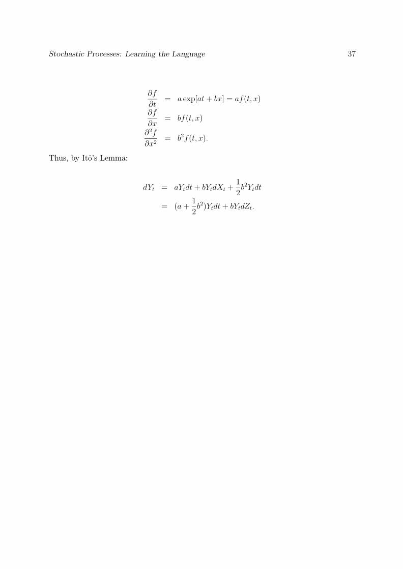
Stochastic Processes: Learning the Language 37
∂f
∂t= a exp[at + bx] = af(t, x)
∂f
∂x= bf(t, x)
∂2f
∂x2= b2f(t, x).
Thus, by Ito’s Lemma:
dYt = aYtdt + bYtdXt +1
2b2Ytdt
= (a +1
2b2)Ytdt + bYtdZt.