stochastic modeling of molecular reaction networks

Stochastic modeling of molecular reaction networks

Daniel Forger

University of Michigan

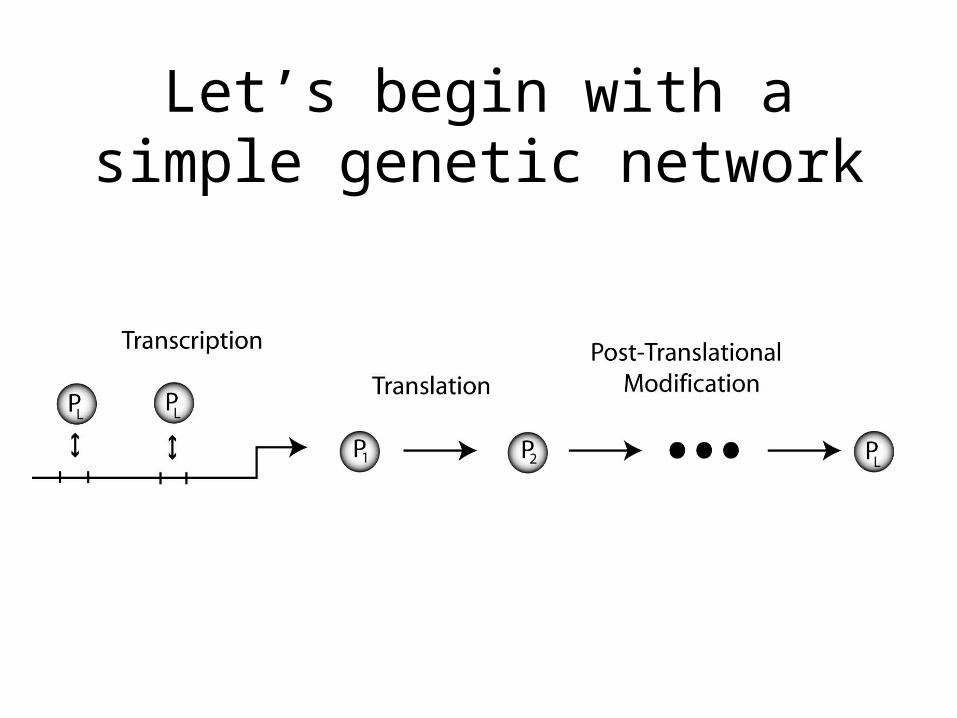
Let’s begin with a simple genetic network

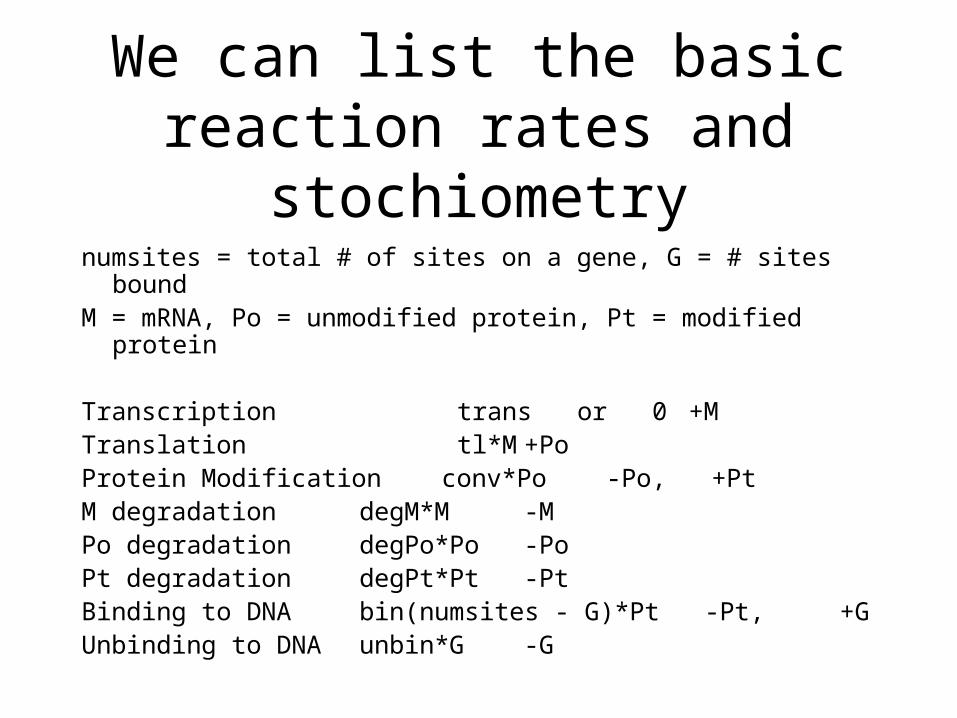
We can list the basic reaction rates and stochiometry

numsites = total # of sites on a gene, G = # sites bound M = mRNA, Po = unmodified protein, Pt = modified protein

Transcription trans or 0 +MTranslation tl*M +PoProtein Modification conv*Po -Po, +PtM degradation degM*M -MPo degradation degPo*Po -PoPt degradation degPt*Pt -PtBinding to DNA bin(numsites - G)*Pt -Pt, +GUnbinding to DNA unbin*G -G

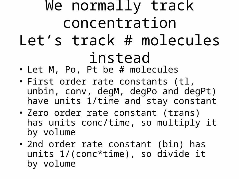
We normally track concentrationLet’s track # molecules instead

• Let M, Po, Pt be # molecules• First order rate constants (tl, unbin, conv,

degM, degPo and degPt) have units 1/time and stay constant

• Zero order rate constant (trans) has units conc/time, so multiply it by volume

• 2nd order rate constant (bin) has units 1/(conc*time), so divide it by volume

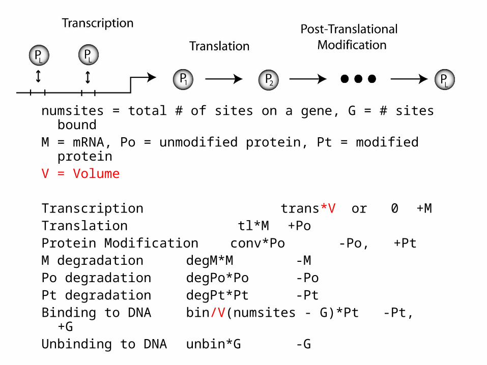
numsites = total # of sites on a gene, G = # sites bound M = mRNA, Po = unmodified protein, Pt = modified proteinV = Volume

Transcription trans*V or 0 +MTranslation tl*M +PoProtein Modification conv*Po -Po, +PtM degradation degM*M -MPo degradation degPo*Po -PoPt degradation degPt*Pt -PtBinding to DNA bin/V(numsites - G)*Pt -Pt, +GUnbinding to DNA unbin*G -G

How would you simulate this?

• Choose which reaction happens next– Find next reaction– Update species by stochiometry of next

reaction– Find time to this next reaction

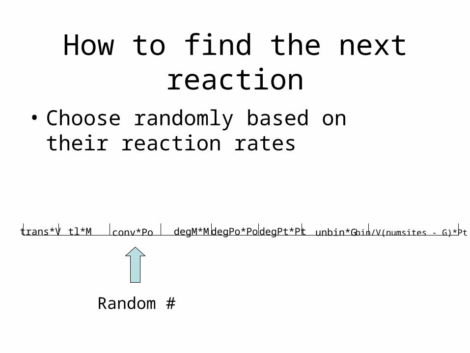
How to find the next reaction

• Choose randomly based on their reaction rates

trans*V tl*M conv*Po degM*M degPo*Po degPt*Pt bin/V(numsites - G)*Ptunbin*G

Random #

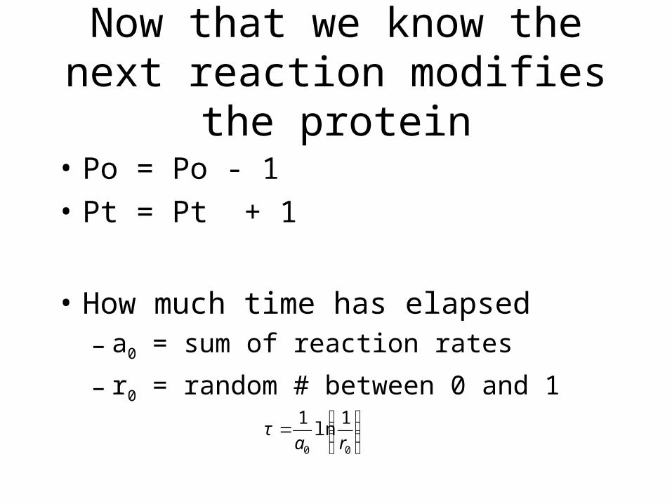
Now that we know the next reaction modifies the protein

• Po = Po - 1

• Pt = Pt + 1

• How much time has elapsed– a0 = sum of reaction rates

– r0 = random # between 0 and 1

⎟⎟⎠

⎞⎜⎜⎝

⎛=

00

1ln

1

raτ

This method goes by many names

• Computational Biologists typically call this the Gillespie Method– Gillespie also has another method

• Material Scientists typically call this Kinetic Monte Carlo

Myth 1:“Mass Action Formulations do not account for Stochasticity”

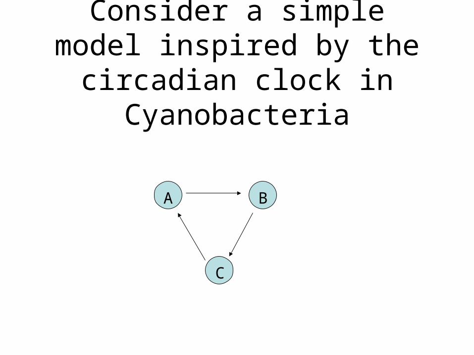
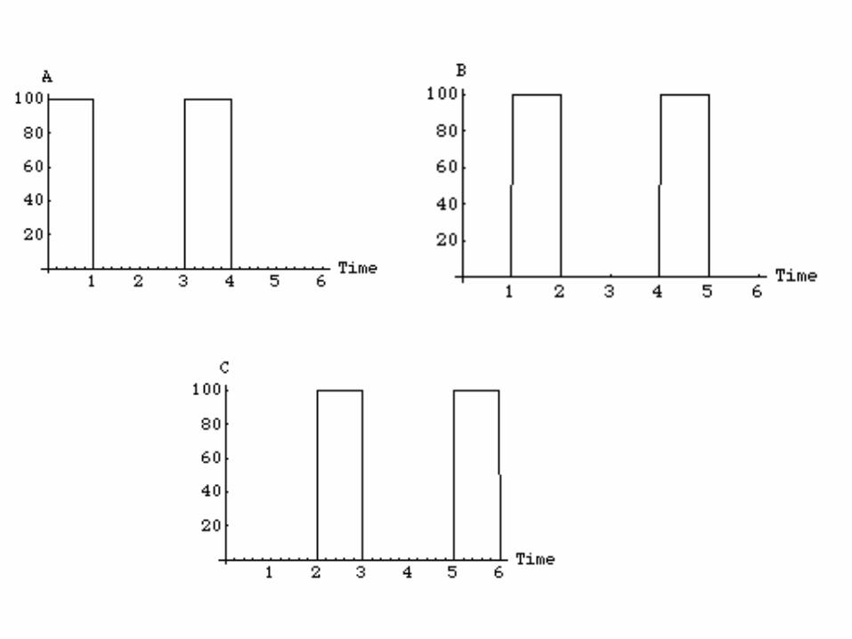
Consider a simple model inspired by the circadian clock

in Cyanobacteria

A B

C

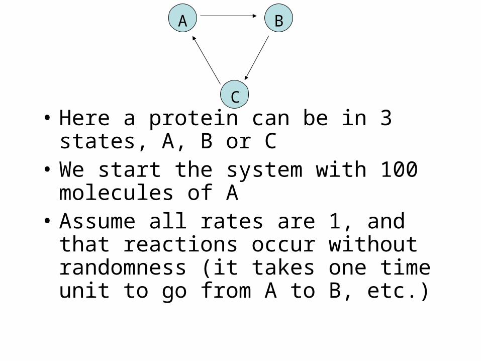
• Here a protein can be in 3 states, A, B or C

• We start the system with 100 molecules of A

• Assume all rates are 1, and that reactions occur without randomness (it takes one time unit to go from A to B, etc.)

A B

C

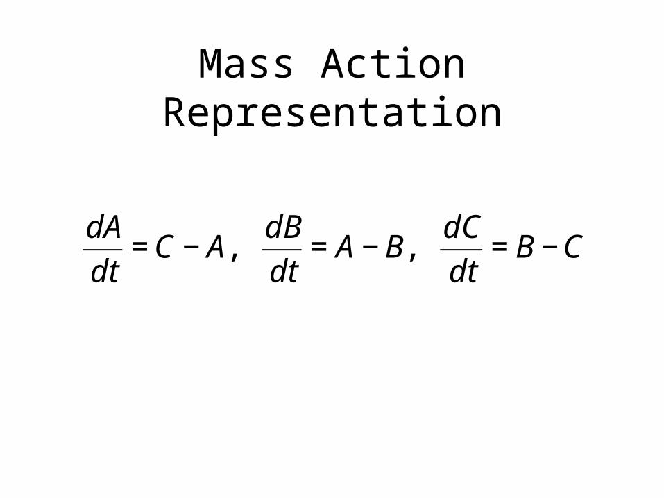
Mass Action Representation

€

dA

dt= C − A,

dB

dt= A − B,

dC

dt= B − C

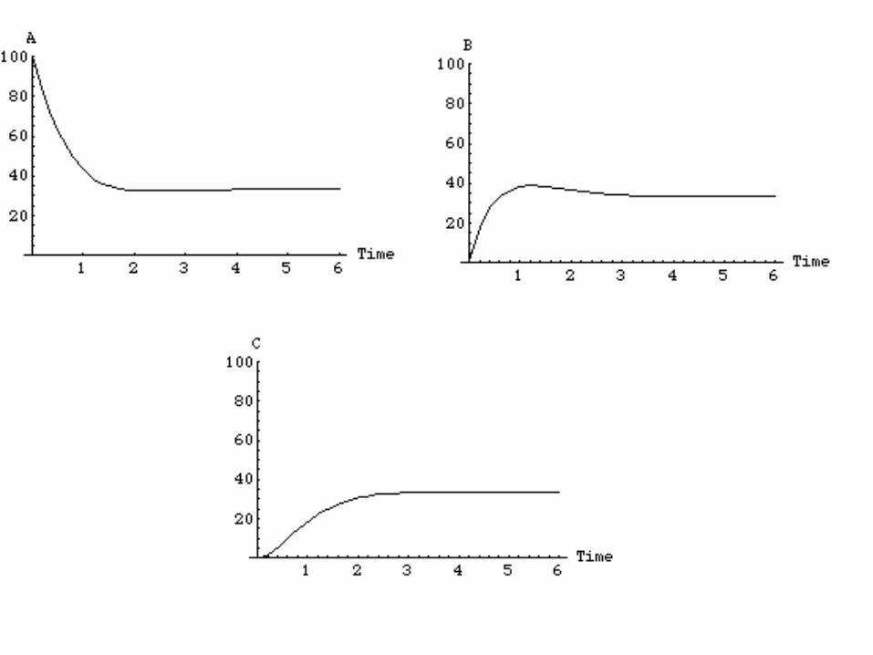
Matlab simulation

Mass Action represents a limiting case of Stochastics

• Mass action and stochastic simulations should agree when certain “limits” are obtained

• Mass action typically represents the expected concentrations of chemical species (more later)

Myth 2:Stochastic and Mass Action

Approaches agree only if there are enough molecules

What matters is the number of reactions

• This is particularly important for reversible reactions

• By the central limit theorem, fluctuations dissapear like n-1/2

• There are almost always a very limited number of genes, – Ok if fast binding and unbinding

There are several representations in between Mass Action and Gillespie

• Chemical Langevin Equations

• Master Equations

• Fokker-Planck

• Moment descriptions

We will illustrate this with an exampleKepler and Elston Biophysical Journal 81:3116

QuickTime™ and aTIFF (Uncompressed) decompressor

are needed to see this picture.

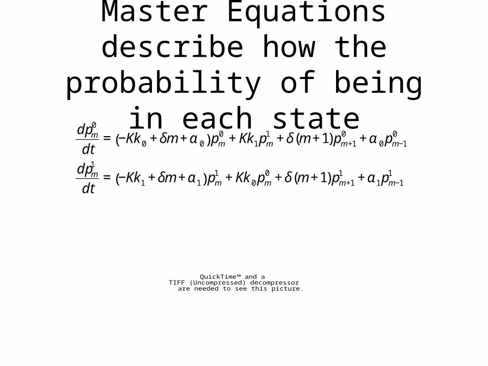
Master Equations describe how the probability of being in

each state

€

dpm0

dt= −Kk0 + δm + α 0( ) pm

0 + Kk1pm1 + δ(m +1)pm +1

0 + α 0 pm−10

dpm1

dt= −Kk1 + δm + α 1( ) pm

1 + Kk0 pm0 + δ(m +1)pm +1

1 + α 1pm−11



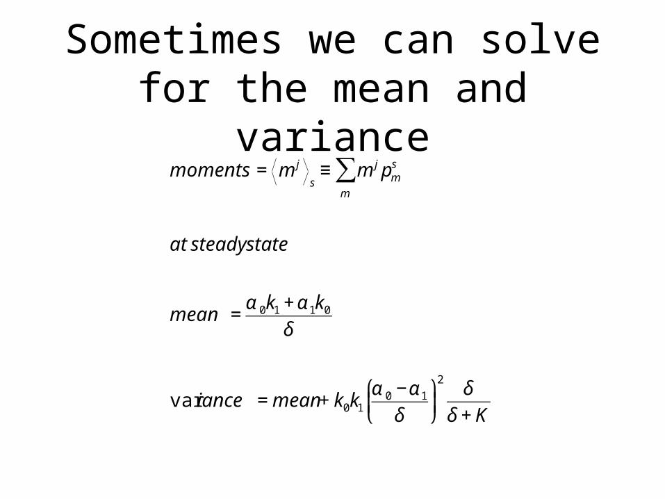
Sometimes we can solve for the mean and variance

€

moments = m j

s≡ m j pm

s

m

∑

at steady state

mean =α 0k1 + α 1k0

δ

var iance = mean + k0k1

α 0 −α 1

δ

⎛

⎝ ⎜

⎞

⎠ ⎟2

δ

δ + K

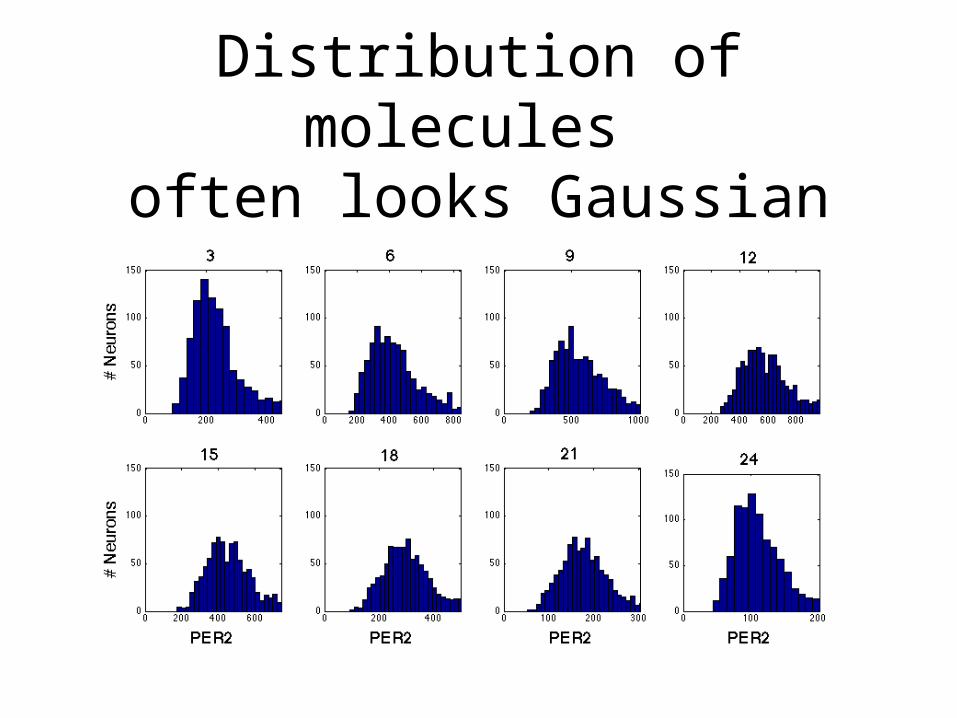
Distribution of molecules often looks Gaussian

Moment Descriptions

• Gaussian Random Variables are fully characterized by their mean and standard deviation

• We can write down odes for the mean and standard deviation of each variable

• However, for bimolecular reactions, we need to know the correlations between variables (potentially N2)

Towards Fokker Planck

• Let’s divide the master equation by the mean m*.

• Although this equation described many states, we can smooth the states to make a probability distribution function

€

pms (t) ≡ dxps(x, t)

(m−1/ 2)/ m*

(m +1/ 2)/ m*

∫

Note

€

ps x +1

m*

⎛

⎝ ⎜

⎞

⎠ ⎟=

1

j!∂x( )

jps(x)

1

m*

⎛

⎝ ⎜

⎞

⎠ ⎟j

= e1

m*∂ x

ps(x)j

∑

If 1/m* is small, we can then derive a simplifedVersion of the Master equations

€

∂t ps(x) = −∂x

α s

m*−δx

⎛

⎝ ⎜

⎞

⎠ ⎟ps(x)

⎡

⎣ ⎢

⎤

⎦ ⎥+

1

2m*∂x

2 α s

m*+ δx

⎛

⎝ ⎜

⎞

⎠ ⎟ps(x)

⎡

⎣ ⎢

⎤

⎦ ⎥+ K[k ˆ s pˆ s (x) − ks ps(x)]

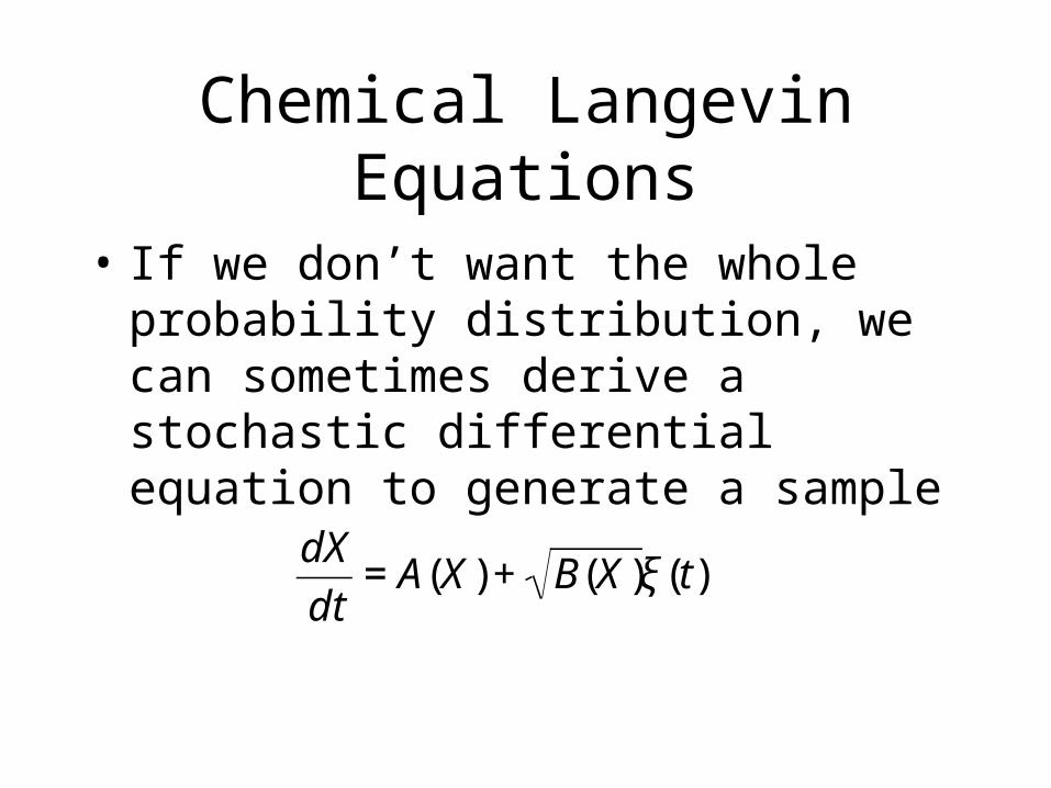
Chemical Langevin Equations

• If we don’t want the whole probability distribution, we can sometimes derive a stochastic differential equation to generate a sample

€

dX

dt= A(X) + B(X)ξ (t)

Adalsteinsson et al. BMC Bioinformatics 5:24



Examples

• Transcription Control

• Lac Operon

• Oscillations

• Accounting for diffusion

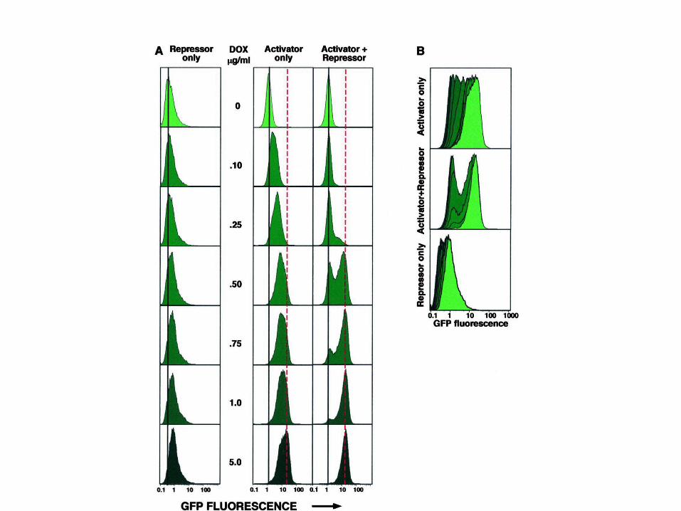
Rossi et al. Molecular Cell



Ozbudak et al. Nature 427:737



Guantes and Poyatos PLoS Computational Biology 2:e30



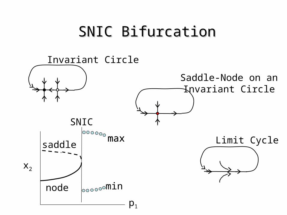
SNIC BifurcationSNIC Bifurcation

Invariant Circle

Limit Cycle

x2

p1

node

saddle

Saddle-Node on anInvariant Circle

max

min

max

SNIC

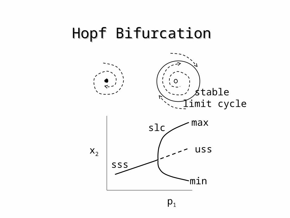
Hopf BifurcationHopf Bifurcation

x2

p1

stable limit cycle

sss

uss

slc max

min

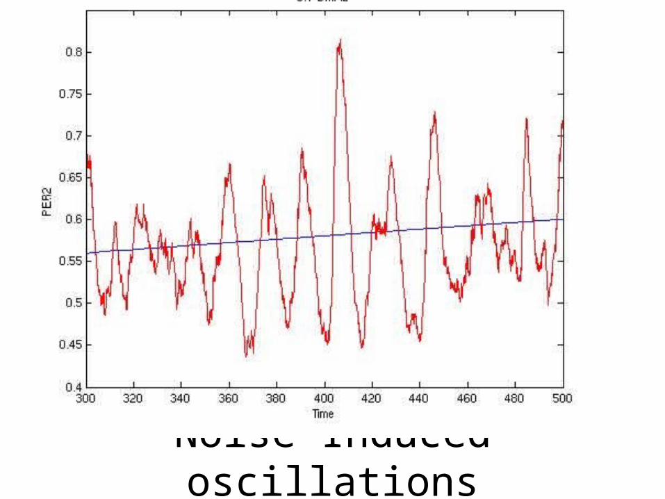
Noise Induced oscillations

Liu et al. Cell 129:605



3-D Gillespie

http://www.math.utah.edu/~isaacson/3dmodel.html

stochastic modeling of molecular reaction networks

Documents