stochastic modeling of carcinogenesis - mathematicsmillerpd/docs/501_fall12/rafaelmezaaim... ·...

Stochastic modeling of carcinogenesis

Rafael Meza Department of Epidemiology

University of Michigan SPH-II 5533

[email protected] http://www.sph.umich.edu/faculty/rmeza.html

Outline

•  Multistage carcinogenesis models

•  Examples

•  Potential projects

Multistage Carcinogenesis Models

Multistage Carcinogenesis

•  Cancer is the consequence of the accumulation of genetic transformations in a single cell (or its descendants)

•  Mueller (1951) & Nordling (1953) (before DNA structure discovery!)

•  Armitage-Doll Model (1954); TSCE Model (1979)

•  Mechanistic models (biologically based) –  Cancer epidemiology –  Laboratory experiments

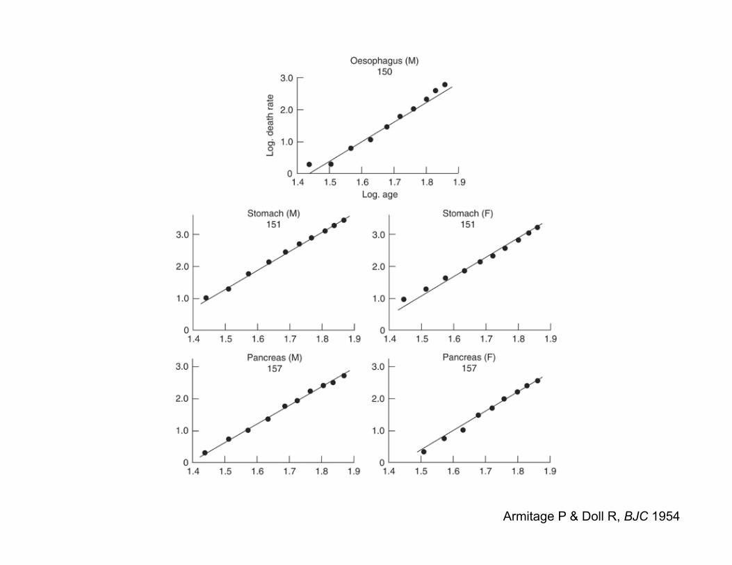
Armitage P & Doll R, BJC 1954

Armitage-Doll Model (1954)

Exponential waiting time

E0 E1 E2 En λ0 λ1 λ2 λn-1

Normal Stem Cell

Malignant Cell


€

Let pk (a) be the probability that the cell is at stage kat age a

)()(

)()()(

)()(

11

11001

000

apdaadp

apapdaadp

apdaadp

nnn

−−=

−=

−=

λ

λλ

λ


( )Nn apaSaP

N

)(1)(] ageby cancer No[

:cells stem esusceptibl are thereAssume

−==

Cancer hazard (age-specific cancer risk):

h(a) = −d ln S(a)[ ]

da≈Nλ0λ1λn−1a

n−1

(n−1)!

Armitage-Doll Model (1954) Age-Specific Incidence

)log()1()!1(

log))(log( 110 ann

Nah n −+⎟⎟⎠

⎞⎜⎜⎝

⎛

−≈ −λλλ …

Armitage P & Doll R, BJC 1954

Hazard or Incidence Function (Measure of Cancer Risk)

•  The hazard is a theoretical representation of the observed incidence or mortality of cancer in the population (# of cases(a) / population(a))

•  Mathematically it measures the instantaneous probability of getting (dying from) cancer

•  Carcinogenesis model à Derive hazard/survival à Estimate model parameters by fitting to cancer incidence/mortality dataà …

TSCE Model (1979)

•  Knudson’s hypothesis (early 70’s): –  Two hits are needed for the retinoblastoma “gene”

to cause a tumor, with this occurring at the somatic level in the sporadic form while one hit is inherited in the familial form

–  Retinoblastoma gene identified in 1987

•  Two Stage Clonal Expansion Model –  Mathematical expression of Knudson’s hypothesis –  Incorporates clonal expansion of pre-malignant

cells –  Follows initiation-promotion-progression paradigm

TSCE Model

β(t)

Moolgavkar & Venzon (Math. Biosc, 1979); Moolgavkar & Knudson (JNCI, 1981)

Non-homogeneous Poisson Process

Birth-Death-Mutation Process

with initial condition Ψ(y,z,0)=1

,,

( , , ) ( ) j kj k

j ky z t P t y zΨ ≡∑

Let,

TSCE Model

€

∂Ψ(y,z,t)dt

= (y −1)ν(t)X(t)Ψ(y,z,t)

+ µ(t)z +α(t)y − (α(t)+ β(t)+ µ(t))[ ]y + β(t){ }∂Ψ(y,z,t)dy

As a continuous time Markov Process

Forward-Kolmogorov equation

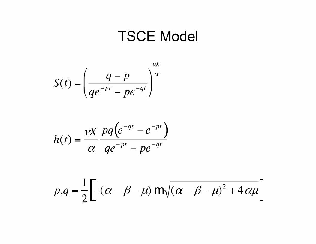
TSCE Model

€

S(t) =q − p

qe− pt − pe−qt⎛

⎝ ⎜

⎞

⎠ ⎟

νXα

h(t) =νXα

pq e−qt − e−pt( )qe− pt − pe−qt

p,q =12−(α − β − µ)m (α − β − µ)2 + 4αµ[ ]

•  Analysis of population level data: –  Closed form expressions for the hazard and survival

functions in case of constant and piecewise constant parameters. Heidenreich et al. (Risk Analysis, 1997)

–  Numerical solution in case of general age-dependent parameters

•  Analysis of experimental data: –  Number and size distribution of premalignant and

malignant lesions

TSCE Model

Generalizations •  Luebeck-Moolgavkar (2002)

•  Tan (1986), Little (1996)

β

Normal X Gatek+/- Gatek-/-

Premalig. Cancer

α

µ0 µ1 µ2

A simple 3-stage Model

Premalignant lesion Onset sojourn time s

€

τ

Φ1(u;a) Φ3(u;a) Φ2(u;a) Ψ(u;a)

3-stage Model

I1 I2 I3 X

Normal X Gatek+/- Gatek-/-

Premalig. Cancer

α

µ0 µ1 µ2

β

As a continuous time branching process

Probability Generating Functions

€

ψ(y1,y2,y3,u;a) = E[y1I1 (a )y2

I 2 (a )y3I 3 (a ) | I1(u) = 0,I2(u) = 0,I3(u) = 0]

Φ1(y1,y2,y3,u;a) = E[y1I1 (a )y2

I 2 (a )y3I 3 (a ) | I1(u) =1,I2(u) = 0,I3(u) = 0]

Φ2(y1,y2,y3,u;a) = E[y1I1 (a )y2

I 2 (a )y3I 3 (a ) | I1(u) = 0,I2(u) =1,I3(u) = 0]

Φ3(y1,y2,y3,u;a) = E[y1I1 (a )y2

I 2 (a )y3I 3 (a ) | I1(u) = 0,I2(u) = 0,I3(u) =1]

Backward Kolmogorov Eqns.

€

∂Ψ u;a( )∂u

= µ0 a − u( )X a − u( )Ψ u;a( ) Φ1 u;a( )−1[ ]

∂Φ1 u;a( )∂u

= µ1 a − u( )Φ1 u;a( ) Φ2 u;a( )−1[ ]

∂Φ2 u;a( )∂u

= β a − u( )+α a − u( )Φ22(u;a)

− α a − u( )+β a − u( )+µ2 a − u( )(1−Φ3(u;a))[ ]Φ2(u;a)

∂Φ3 u;a( )∂u

= 0

€

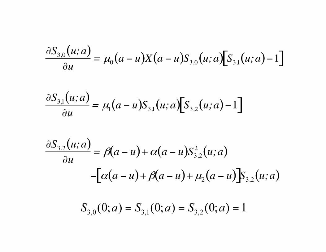
∂S3,0 u;a( )∂u

= µ0 a − u( )X a − u( )S3,0 u;a( ) S3,1 u;a( )−1[ ]

∂S3,1 u;a( )∂u

= µ1 a − u( )S3,1 u;a( ) S3,2 u;a( )−1[ ]

∂S3,2 u;a( )∂u

= β a − u( )+α a − u( )S3,22 u;a( )

− α a − u( )+β a − u( )+µ2 a − u( )[ ]S3,2 u;a( )

1);0();0();0( 2,31,30,3 === aSaSaS

€

S3 a( )= S3,0 a;a( )

= exp µ00

t

∫ Xq − p

qe−p a−u( ) − pe−q a−u( )

⎛

⎝ ⎜

⎞

⎠ ⎟

µ1 /α−1

⎡

⎣

⎢ ⎢

⎤

⎦

⎥ ⎥ du

⎧

⎨ ⎪

⎩ ⎪

⎫

⎬ ⎪

⎭ ⎪

p,q= 12− α − β − µ2( )m α − β − µ2( )2 +4αµ2⎡ ⎣ ⎢

⎤ ⎦ ⎥

€

h3 a( )= −d ln(S3(a))

da

= µ0X 1−q − p

qe− pa − pe−qa⎛

⎝ ⎜

⎞

⎠ ⎟

µ1 /α⎡

⎣

⎢ ⎢

⎤

⎦

⎥ ⎥

3-stage Model Hazard

We can say more with some asymptotic analysis

age-specific cancer incidence

Age (a)

Can

cer I

ncid

ence

€

µ0Xasymptotic value

age-specific cancer incidence - explained

Age (a)

Can

cer I

ncid

ence

€

µ0Xµ1p∞ a −Ts( )Premalignant lesion incidence

Ts


mean sojourn time

Age (a)

Can

cer I

ncid

ence

asymptotic value

€

exp α − β( )a{ }

Prem. lesion growth


Age (a)

Can

cer I

ncid

ence


power law

€

12

µ0Xµ1µ2a2

Age (a)

Can

cer I

ncid

ence

€

µ0Xasymptotic value

€

µ0Xµ1p∞ a −Ts( )Premalignant lesion incidence

Ts €

exp α − β( )a{ }

Prem. lesion growth


power law

€

12

µ0Xµ1µ2a2

mean sojourn time

Age (a)

Can

cer I

ncid

ence

Meza R et al, PNAS 2008

Age Age

Slope=3.9

Slope=2.8

Ts=52.9 Ts=56.3

Age

-spe

cific

Inci

denc

e pe

r 100

K

Males Females

30 40 50 60 70 80 30 40 50 60 70 80

0

20

4

0

60

8

0

100

12

0 Pancreatic Cancer

(“adjusted” incidence)


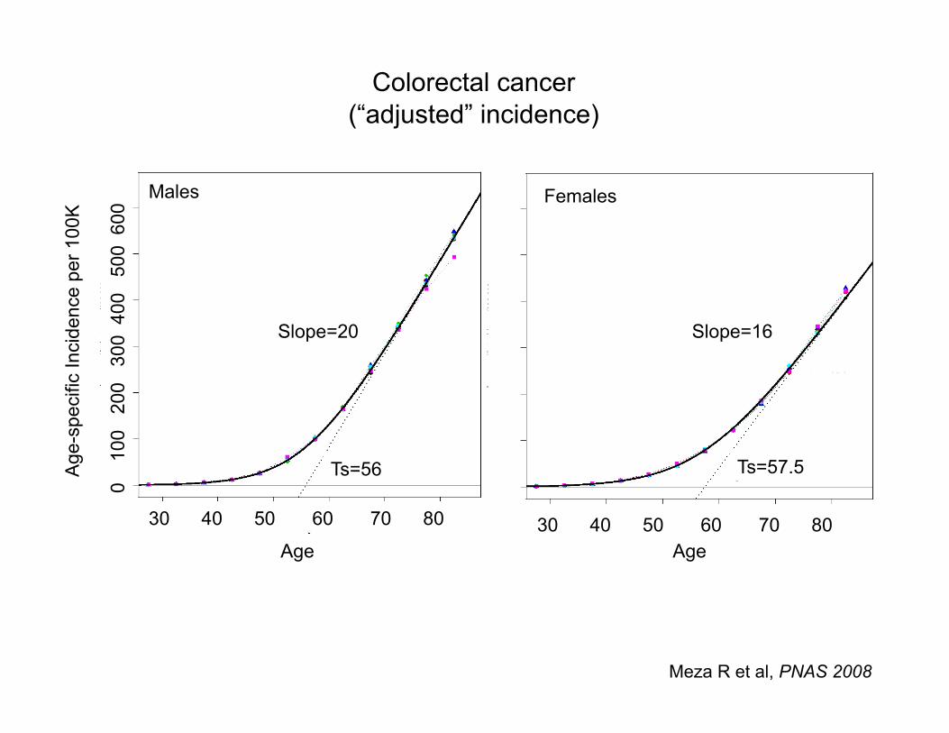
Age Age

Slope=20 Slope=16

Ts=56 Ts=57.5 Age

-spe

cific

Inci

denc

e pe

r 100

K Males Females

30 40 50 60 70 80 30 40 50 60 70 80

0

100

20

0 3

00 4

00

500

600

Colorectal cancer (“adjusted” incidence)


CURRENT PROJECTS

Lung cancer screening

•  Does LC screening among ‘heavy smokers’ reduce LC mortality – Yes, with low dose CT screening – One big –expensive -trial has shown

•  Extrapolate results of the trial – Model relationship of smoking and LC – Effects of screening –  Impact of radiation dose

Preclinical

Normal X Preini.ated Pre

malignant

αpm βpm

µ0 µ1 Preclinical

αpc βpc

µpm

IA1 IA2 IB II IIIA IIIB IV

Clinical Detec.on

λIA1 λIA2 λIB λII λIIIA λIIIB

δIA1 δIA2 δIB δII δIIIA δIIIB δIV

Michigan/FHCRC Lung Cancer screening model. By gender and histology (SC,AC,SQ,ONSCLC)

37

Infec.ous agents and cancer

•  Two disease processes with very different scales – Popula.on vs individual

– Days vs years

– Persons vs cells/genes

38

S E I R βSI/N νE γI

b

d d

A. Population level (SEIR Model)

B. Individual level (Multistage Carcinogenesis Model)

Normal X Gatek+/- Gatek-/- Cancer

α β

µ0 µ1 µ2

INFECTIOUS AGENT

INFECTIOUS AGENT

increase cell division

reduce apoptosis

increase mutation rates

d d

Cancer evolution

•  Use new genetic data to infer the natural history and the dynamics of carcinogenesis

•  Constrained by what’s known at the population level

Conclusions

•  Multistage carcinogenesis models - powerful framework for cancer risk analysis

•  Complement to traditional statistical and epidemiological approaches – mechanistic models

•  Allows “direct” interpretation of results in terms of potential biological mechanisms

•  Nice applied math area : stochastic modeling, dynamical systems, PDEs, ODEs, numerical analysis, statistics

Conclusions •  Other applications:

–  Radiation risk assessment

–  Toxicology

–  Developmental mutations and cancer risk

–  Public health policy

Conclusions

•  Second cancers after radio- and chemo-therapy

•  Cancers with infectious disease etiology

•  Genomic, epigenomic and proteomic data

•  Link between biological complexity and “simplicity” observed in public level data –  multi-scale modeling –  integrative cancer biology

•  Armitage P & Doll R. The age distribution of cancer and multistage theory of carcinogenesis. British J. Cancer 8:1-12, 1954

•  Whittemore A & Keller JB. Quantitative theories of carcinogenesis. SIAM Review 20, 1978.

•  Moolgavkar SH & Venzon DJ. Two-event models for carcinogenesis: incidence curves for childhood and adult tumors. Mathematical Biosciences 47:55-77, 1979

•  Moolgavkar SH & Knudson A. Mutation and cancer: a model for human carcinogenesis. J Natl Cancer Inst. 66:1037-52, 1981

•  Kopp-Schneider A. Carcinogenesis models for risk assessment. Stat. Methods Med. Res. 6: 317-340, 1997

•  Luebeck EG & Moolgavkar SH. Multistage carcinogenesis and the incidence of colorectal cancer. PNAS 99:15095-15100, 2002

•  Meza R, Luebeck EG & Moolgavkar SH. Gestational mutations and carcinogenesis. Mathematical Biosciences 197:188-210, 2005.

•  Meza R, Jeon J, Moolgavkar SH & Luebeck EG. Age-specific incidence of cancer: Phases,

transitions, and biological implications. PNAS 105:16284-9, 2008 •  Meza R, Jeon J, Renehan AG, Luebeck EG (Jul 2010) Colorectal Cancer Incidence Trends in

the United States and United Kingdom: Evidence of Right- to Left-Sided Biological Gradients with Implications for Screening., Cancer research, 70 (13), 5419-5429

stochastic modeling of carcinogenesis - mathematicsmillerpd/docs/501_fall12/rafaelmezaaim... ·...

Documents