stochastic lot-sizing problem: a joint chance-constrained ...jfro/journeesprecedentes/... ·...
TRANSCRIPT

Stochastic lot-sizing problem: a joint chance-constrainedprogramming approach
Celine Gicquel 1, Jianqiang Cheng 1
1Laboratoire de Recherche en InformatiqueUniversite Paris Sud
JFRO - Nov. 2014
C. Gicquel, LRI, Universite Paris Sud Stochastic lot-sizing JFRO - Nov. 2014 1 / 35
Plan
1 Deterministic lot-sizing problem
2 Stochastic lot-sizing problem
3 Sample approximation approach
4 Partial sample approximation approach
5 Preliminary computational results
6 Conclusion and perspectives
C. Gicquel, LRI, Universite Paris Sud Stochastic lot-sizing JFRO - Nov. 2014 2 / 35
Deterministic lot-sizing problem
Plan
1 Deterministic lot-sizing problem
2 Stochastic lot-sizing problem
3 Sample approximation approach
4 Partial sample approximation approach
5 Preliminary computational results
6 Conclusion and perspectives
C. Gicquel, LRI, Universite Paris Sud Stochastic lot-sizing JFRO - Nov. 2014 3 / 35

Deterministic lot-sizing problem
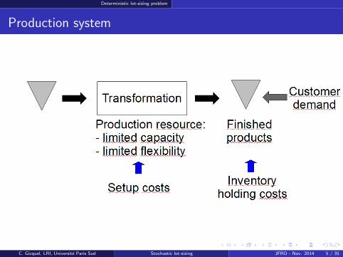
Production system
C. Gicquel, LRI, Universite Paris Sud Stochastic lot-sizing JFRO - Nov. 2014 4 / 35
Deterministic lot-sizing problem
Production system
C. Gicquel, LRI, Universite Paris Sud Stochastic lot-sizing JFRO - Nov. 2014 5 / 35

Deterministic lot-sizing problem
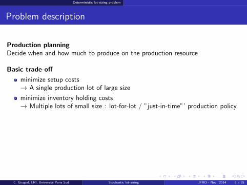
Problem description
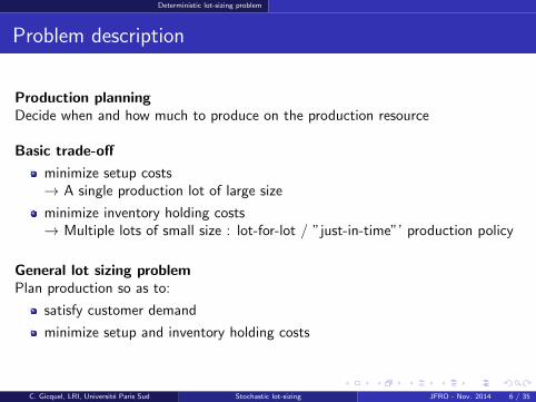
Production planningDecide when and how much to produce on the production resource
Basic trade-off
minimize setup costs→ A single production lot of large size
minimize inventory holding costs→ Multiple lots of small size : lot-for-lot / ”just-in-time”’ production policy
General lot sizing problemPlan production so as to:
satisfy customer demand
minimize setup and inventory holding costs
C. Gicquel, LRI, Universite Paris Sud Stochastic lot-sizing JFRO - Nov. 2014 6 / 35
Deterministic lot-sizing problem
Problem description
Production planningDecide when and how much to produce on the production resource
Basic trade-off
minimize setup costs→ A single production lot of large size
minimize inventory holding costs→ Multiple lots of small size : lot-for-lot / ”just-in-time”’ production policy
General lot sizing problemPlan production so as to:
satisfy customer demand
minimize setup and inventory holding costs
C. Gicquel, LRI, Universite Paris Sud Stochastic lot-sizing JFRO - Nov. 2014 6 / 35
Deterministic lot-sizing problem
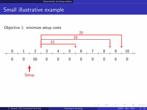
Small illustrative example
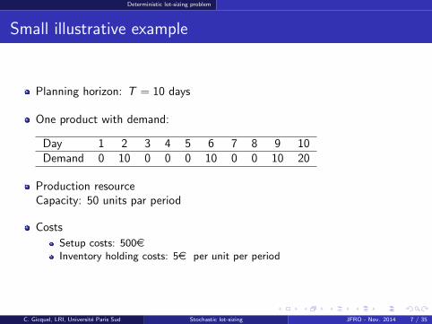
Planning horizon: T = 10 days
One product with demand:
Day 1 2 3 4 5 6 7 8 9 10Demand 0 10 0 0 0 10 0 0 10 20
Production resourceCapacity: 50 units par period
Costs
Setup costs: 500eInventory holding costs: 5e per unit per period
C. Gicquel, LRI, Universite Paris Sud Stochastic lot-sizing JFRO - Nov. 2014 7 / 35
Deterministic lot-sizing problem
Small illustrative example
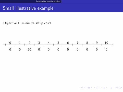
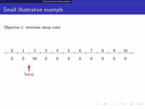
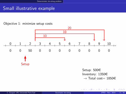
Objective 1: minimize setup costs
0 1 2 3 4 5 6 7 8 9 10
0 0 50 0 0 0 0 0 0 0 0
Setup
1010
20
Setup: 500eInventory: 1350e→ Total cost= 1850e
C. Gicquel, LRI, Universite Paris Sud Stochastic lot-sizing JFRO - Nov. 2014 8 / 35
Deterministic lot-sizing problem
Small illustrative example
Objective 1: minimize setup costs
0 1 2 3 4 5 6 7 8 9 10
0 0 50 0 0 0 0 0 0 0 0
Setup
1010
20
Setup: 500eInventory: 1350e→ Total cost= 1850e
C. Gicquel, LRI, Universite Paris Sud Stochastic lot-sizing JFRO - Nov. 2014 8 / 35
Deterministic lot-sizing problem
Small illustrative example
Objective 1: minimize setup costs
0 1 2 3 4 5 6 7 8 9 10
0 0 50 0 0 0 0 0 0 0 0
Setup
1010
20
Setup: 500eInventory: 1350e→ Total cost= 1850e
C. Gicquel, LRI, Universite Paris Sud Stochastic lot-sizing JFRO - Nov. 2014 8 / 35
Deterministic lot-sizing problem
Small illustrative example
Objective 1: minimize setup costs
0 1 2 3 4 5 6 7 8 9 10
0 0 50 0 0 0 0 0 0 0 0
Setup
1010
20
Setup: 500eInventory: 1350e→ Total cost= 1850e
C. Gicquel, LRI, Universite Paris Sud Stochastic lot-sizing JFRO - Nov. 2014 8 / 35
Deterministic lot-sizing problem
Small illustrative example
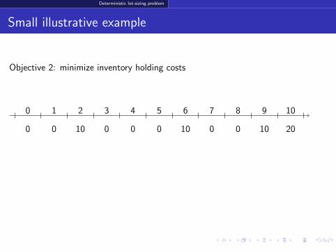
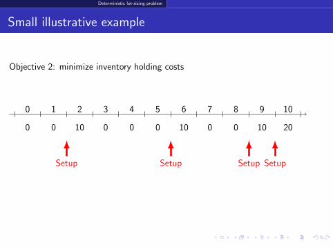
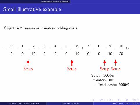
Objective 2: minimize inventory holding costs
0 1 2 3 4 5 6 7 8 9 10
0 0 10 0 0 0 10 0 0 10 20
Setup Setup Setup Setup
Setup: 2000eInventory: 0e→ Total cost= 2000e
C. Gicquel, LRI, Universite Paris Sud Stochastic lot-sizing JFRO - Nov. 2014 9 / 35
Deterministic lot-sizing problem
Small illustrative example
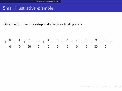
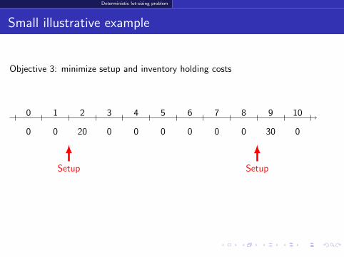
Objective 3: minimize setup and inventory holding costs
0 1 2 3 4 5 6 7 8 9 10
0 0 20 0 0 0 0 0 0 30 0
Setup Setup
10 20
Setup: 1000eInventory: 250e→ Total cost= 1250 e
C. Gicquel, LRI, Universite Paris Sud Stochastic lot-sizing JFRO - Nov. 2014 10 / 35
Deterministic lot-sizing problem
Small illustrative example
Objective 3: minimize setup and inventory holding costs
0 1 2 3 4 5 6 7 8 9 10
0 0 20 0 0 0 0 0 0 30 0
Setup Setup
10 20
Setup: 1000eInventory: 250e→ Total cost= 1250 e
C. Gicquel, LRI, Universite Paris Sud Stochastic lot-sizing JFRO - Nov. 2014 10 / 35
Deterministic lot-sizing problem
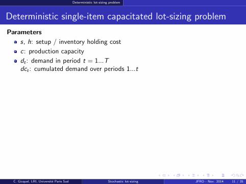
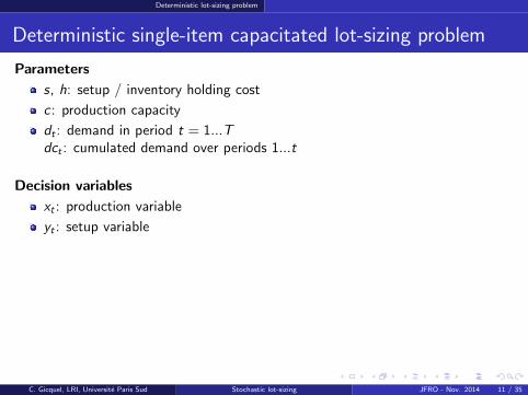
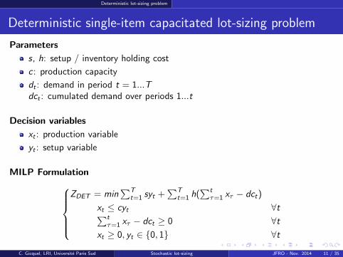
Deterministic single-item capacitated lot-sizing problem
Parameters
s, h: setup / inventory holding cost
c : production capacity
dt : demand in period t = 1...Tdct : cumulated demand over periods 1...t
Decision variables
xt : production variable
yt : setup variable
MILP FormulationZDET = min
∑Tt=1 syt +
∑Tt=1 h(
∑tτ=1 xτ − dct)
xt ≤ cyt ∀t∑tτ=1 xτ − dct ≥ 0 ∀t
xt ≥ 0, yt ∈ {0, 1} ∀t
C. Gicquel, LRI, Universite Paris Sud Stochastic lot-sizing JFRO - Nov. 2014 11 / 35
Deterministic lot-sizing problem
Deterministic single-item capacitated lot-sizing problem
Parameters
s, h: setup / inventory holding cost
c : production capacity
dt : demand in period t = 1...Tdct : cumulated demand over periods 1...t
Decision variables
xt : production variable
yt : setup variable
MILP FormulationZDET = min
∑Tt=1 syt +
∑Tt=1 h(
∑tτ=1 xτ − dct)
xt ≤ cyt ∀t∑tτ=1 xτ − dct ≥ 0 ∀t
xt ≥ 0, yt ∈ {0, 1} ∀t
C. Gicquel, LRI, Universite Paris Sud Stochastic lot-sizing JFRO - Nov. 2014 11 / 35
Stochastic lot-sizing problem
Plan
1 Deterministic lot-sizing problem
2 Stochastic lot-sizing problem
3 Sample approximation approach
4 Partial sample approximation approach
5 Preliminary computational results
6 Conclusion and perspectives
C. Gicquel, LRI, Universite Paris Sud Stochastic lot-sizing JFRO - Nov. 2014 12 / 35
Stochastic lot-sizing problem
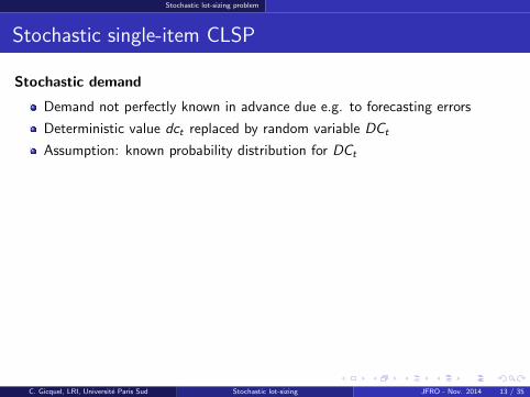
Stochastic single-item CLSP
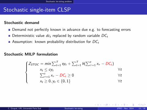
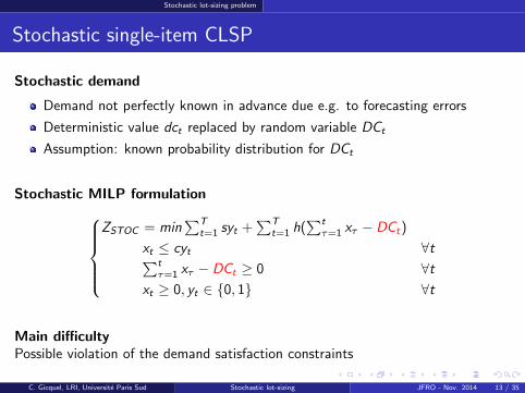
Stochastic demand
Demand not perfectly known in advance due e.g. to forecasting errors
Deterministic value dct replaced by random variable DCt
Assumption: known probability distribution for DCt
Stochastic MILP formulationZSTOC = min
∑Tt=1 syt +
∑Tt=1 h(
∑tτ=1 xτ − DCt)
xt ≤ cyt ∀t∑tτ=1 xτ − DCt ≥ 0 ∀t
xt ≥ 0, yt ∈ {0, 1} ∀t
Main difficultyPossible violation of the demand satisfaction constraints
C. Gicquel, LRI, Universite Paris Sud Stochastic lot-sizing JFRO - Nov. 2014 13 / 35
Stochastic lot-sizing problem
Stochastic single-item CLSP
Stochastic demand
Demand not perfectly known in advance due e.g. to forecasting errors
Deterministic value dct replaced by random variable DCt
Assumption: known probability distribution for DCt
Stochastic MILP formulationZSTOC = min
∑Tt=1 syt +
∑Tt=1 h(
∑tτ=1 xτ − DCt)
xt ≤ cyt ∀t∑tτ=1 xτ − DCt ≥ 0 ∀t
xt ≥ 0, yt ∈ {0, 1} ∀t
Main difficultyPossible violation of the demand satisfaction constraints
C. Gicquel, LRI, Universite Paris Sud Stochastic lot-sizing JFRO - Nov. 2014 13 / 35
Stochastic lot-sizing problem
Modeling alternatives: stockout risk management
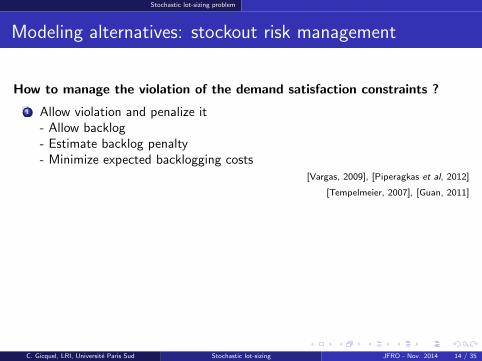
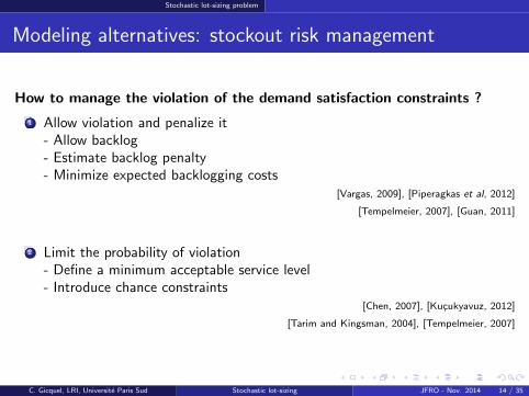
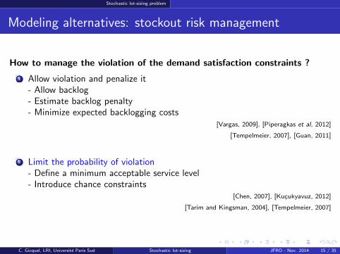
How to manage the violation of the demand satisfaction constraints ?
1 Allow violation and penalize it- Allow backlog- Estimate backlog penalty- Minimize expected backlogging costs
[Vargas, 2009], [Piperagkas et al, 2012]
[Tempelmeier, 2007], [Guan, 2011]
2 Limit the probability of violation- Define a minimum acceptable service level- Introduce chance constraints
[Chen, 2007], [Kucukyavuz, 2012]
[Tarim and Kingsman, 2004], [Tempelmeier, 2007]
C. Gicquel, LRI, Universite Paris Sud Stochastic lot-sizing JFRO - Nov. 2014 14 / 35
Stochastic lot-sizing problem
Modeling alternatives: stockout risk management
How to manage the violation of the demand satisfaction constraints ?
1 Allow violation and penalize it- Allow backlog- Estimate backlog penalty- Minimize expected backlogging costs
[Vargas, 2009], [Piperagkas et al, 2012]
[Tempelmeier, 2007], [Guan, 2011]
2 Limit the probability of violation- Define a minimum acceptable service level- Introduce chance constraints
[Chen, 2007], [Kucukyavuz, 2012]
[Tarim and Kingsman, 2004], [Tempelmeier, 2007]
C. Gicquel, LRI, Universite Paris Sud Stochastic lot-sizing JFRO - Nov. 2014 15 / 35
Stochastic lot-sizing problem
Individual chance constraints
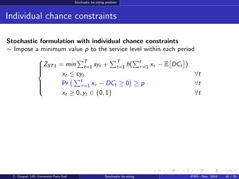
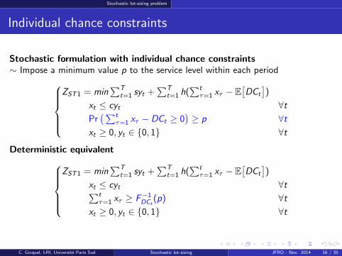
Stochastic formulation with individual chance constraints∼ Impose a minimum value p to the service level within each period
ZST1 = min∑T
t=1 syt +∑T
t=1 h(∑t
τ=1 xτ − E[DCt
])
xt ≤ cyt ∀tPr(∑t
τ=1 xτ − DCt ≥ 0)≥ p ∀t
xt ≥ 0, yt ∈ {0, 1} ∀t
Deterministic equivalentZST1 = min
∑Tt=1 syt +
∑Tt=1 h(
∑tτ=1 xτ − E
[DCt
])
xt ≤ cyt ∀t∑tτ=1 xτ ≥ F−1
DCt(p) ∀t
xt ≥ 0, yt ∈ {0, 1} ∀t
C. Gicquel, LRI, Universite Paris Sud Stochastic lot-sizing JFRO - Nov. 2014 16 / 35
Stochastic lot-sizing problem
Individual chance constraints
Stochastic formulation with individual chance constraints∼ Impose a minimum value p to the service level within each period
ZST1 = min∑T
t=1 syt +∑T
t=1 h(∑t
τ=1 xτ − E[DCt
])
xt ≤ cyt ∀tPr(∑t
τ=1 xτ − DCt ≥ 0)≥ p ∀t
xt ≥ 0, yt ∈ {0, 1} ∀t
Deterministic equivalentZST1 = min
∑Tt=1 syt +
∑Tt=1 h(
∑tτ=1 xτ − E
[DCt
])
xt ≤ cyt ∀t∑tτ=1 xτ ≥ F−1
DCt(p) ∀t
xt ≥ 0, yt ∈ {0, 1} ∀t
C. Gicquel, LRI, Universite Paris Sud Stochastic lot-sizing JFRO - Nov. 2014 16 / 35
Stochastic lot-sizing problem
Joint chance constraints
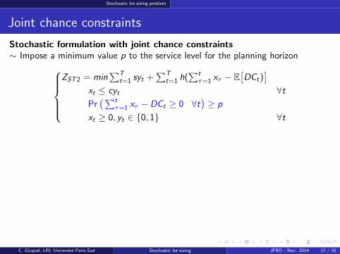
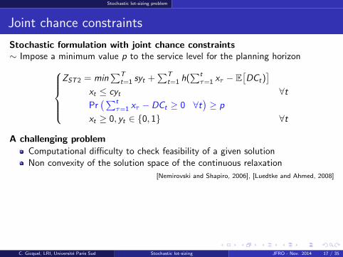
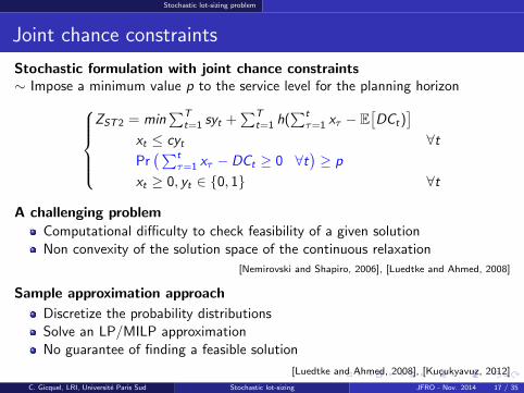
Stochastic formulation with joint chance constraints∼ Impose a minimum value p to the service level for the planning horizon
ZST2 = min∑T
t=1 syt +∑T
t=1 h(∑t
τ=1 xτ − E[DCt)
]xt ≤ cyt ∀tPr(∑t
τ=1 xτ − DCt ≥ 0 ∀t)≥ p
xt ≥ 0, yt ∈ {0, 1} ∀t
A challenging problem
Computational difficulty to check feasibility of a given solutionNon convexity of the solution space of the continuous relaxation
[Nemirovski and Shapiro, 2006], [Luedtke and Ahmed, 2008]
Sample approximation approach
Discretize the probability distributionsSolve an LP/MILP approximationNo guarantee of finding a feasible solution
[Luedtke and Ahmed, 2008], [Kucukyavuz, 2012]
C. Gicquel, LRI, Universite Paris Sud Stochastic lot-sizing JFRO - Nov. 2014 17 / 35
Stochastic lot-sizing problem
Joint chance constraints
Stochastic formulation with joint chance constraints∼ Impose a minimum value p to the service level for the planning horizon
ZST2 = min∑T
t=1 syt +∑T
t=1 h(∑t
τ=1 xτ − E[DCt)
]xt ≤ cyt ∀tPr(∑t
τ=1 xτ − DCt ≥ 0 ∀t)≥ p
xt ≥ 0, yt ∈ {0, 1} ∀t
A challenging problem
Computational difficulty to check feasibility of a given solutionNon convexity of the solution space of the continuous relaxation
[Nemirovski and Shapiro, 2006], [Luedtke and Ahmed, 2008]
Sample approximation approach
Discretize the probability distributionsSolve an LP/MILP approximationNo guarantee of finding a feasible solution
[Luedtke and Ahmed, 2008], [Kucukyavuz, 2012]
C. Gicquel, LRI, Universite Paris Sud Stochastic lot-sizing JFRO - Nov. 2014 17 / 35
Sample approximation approach
Plan
1 Deterministic lot-sizing problem
2 Stochastic lot-sizing problem
3 Sample approximation approach
4 Partial sample approximation approach
5 Preliminary computational results
6 Conclusion and perspectives
C. Gicquel, LRI, Universite Paris Sud Stochastic lot-sizing JFRO - Nov. 2014 18 / 35
Sample approximation approach
Sample approximation for lot-sizing
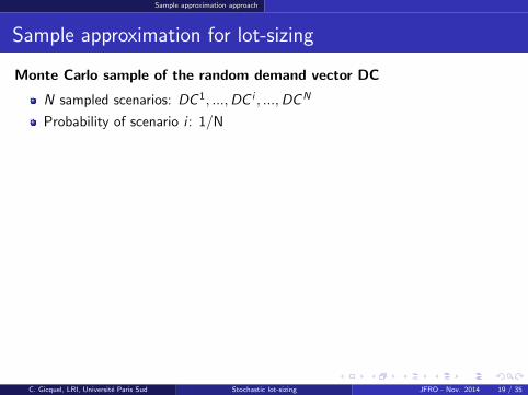
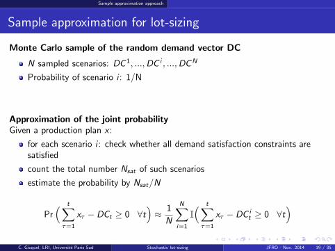
Monte Carlo sample of the random demand vector DC
N sampled scenarios: DC 1, ...,DC i , ...,DCN
Probability of scenario i : 1/N
Approximation of the joint probabilityGiven a production plan x :
for each scenario i : check whether all demand satisfaction constraints aresatisfied
count the total number Nsat of such scenarios
estimate the probability by Nsat/N
Pr( t∑
τ=1
xτ − DCt ≥ 0 ∀t)≈ 1
N
N∑i=1
I( t∑
τ=1
xτ − DC it ≥ 0 ∀t
)
C. Gicquel, LRI, Universite Paris Sud Stochastic lot-sizing JFRO - Nov. 2014 19 / 35
Sample approximation approach
Sample approximation for lot-sizing
Monte Carlo sample of the random demand vector DC
N sampled scenarios: DC 1, ...,DC i , ...,DCN
Probability of scenario i : 1/N
Approximation of the joint probabilityGiven a production plan x :
for each scenario i : check whether all demand satisfaction constraints aresatisfied
count the total number Nsat of such scenarios
estimate the probability by Nsat/N
Pr( t∑
τ=1
xτ − DCt ≥ 0 ∀t)≈ 1
N
N∑i=1
I( t∑
τ=1
xτ − DC it ≥ 0 ∀t
)C. Gicquel, LRI, Universite Paris Sud Stochastic lot-sizing JFRO - Nov. 2014 19 / 35
Sample approximation approach
Sample approximation for lot-sizing
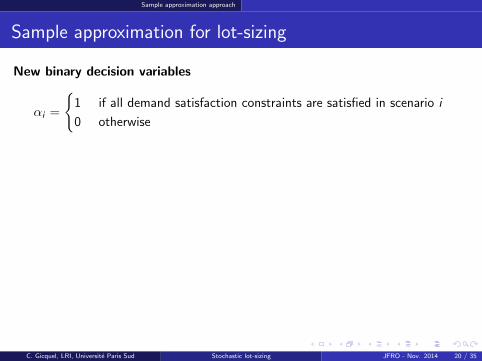
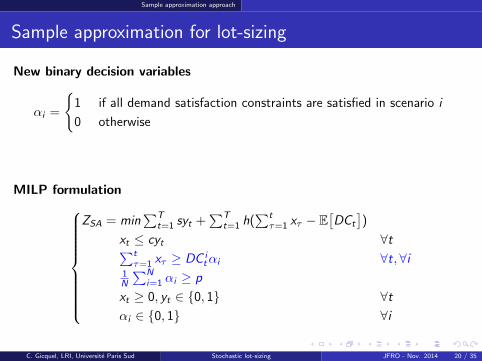
New binary decision variables
αi =
{1 if all demand satisfaction constraints are satisfied in scenario i
0 otherwise
MILP formulation
ZSA = min∑T
t=1 syt +∑T
t=1 h(∑t
τ=1 xτ − E[DCt
])
xt ≤ cyt ∀t∑tτ=1 xτ ≥ DC i
tαi ∀t,∀i1N
∑Ni=1 αi ≥ p
xt ≥ 0, yt ∈ {0, 1} ∀tαi ∈ {0, 1} ∀i
C. Gicquel, LRI, Universite Paris Sud Stochastic lot-sizing JFRO - Nov. 2014 20 / 35
Sample approximation approach
Sample approximation for lot-sizing
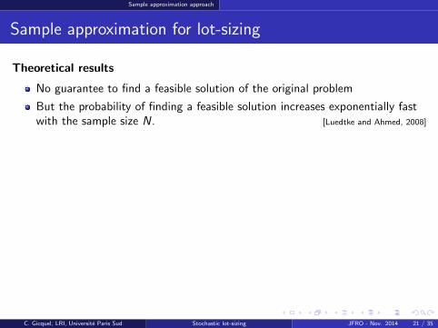
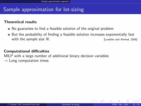
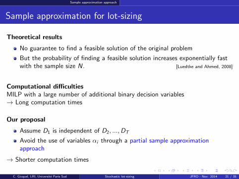
Theoretical results
No guarantee to find a feasible solution of the original problem
But the probability of finding a feasible solution increases exponentially fastwith the sample size N. [Luedtke and Ahmed, 2008]
Computational difficultiesMILP with a large number of additional binary decision variables→ Long computation times
Our proposal
Assume D1 is independent of D2, ...,DT
Avoid the use of variables αi through a partial sample approximationapproach
→ Shorter computation times
C. Gicquel, LRI, Universite Paris Sud Stochastic lot-sizing JFRO - Nov. 2014 21 / 35
Sample approximation approach
Sample approximation for lot-sizing
Theoretical results
No guarantee to find a feasible solution of the original problem
But the probability of finding a feasible solution increases exponentially fastwith the sample size N. [Luedtke and Ahmed, 2008]
Computational difficultiesMILP with a large number of additional binary decision variables→ Long computation times
Our proposal
Assume D1 is independent of D2, ...,DT
Avoid the use of variables αi through a partial sample approximationapproach
→ Shorter computation times
C. Gicquel, LRI, Universite Paris Sud Stochastic lot-sizing JFRO - Nov. 2014 21 / 35
Partial sample approximation approach
Plan
1 Deterministic lot-sizing problem
2 Stochastic lot-sizing problem
3 Sample approximation approach
4 Partial sample approximation approach
5 Preliminary computational results
6 Conclusion and perspectives
C. Gicquel, LRI, Universite Paris Sud Stochastic lot-sizing JFRO - Nov. 2014 22 / 35
Partial sample approximation approach
Partial sample approximation for lot-sizing
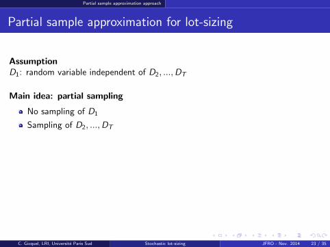
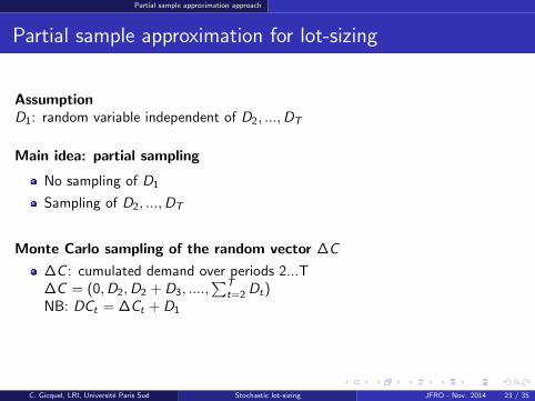
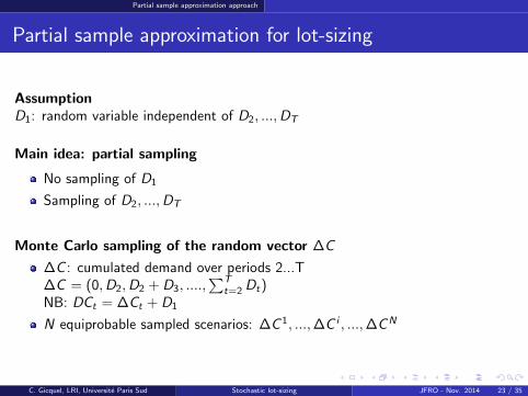
AssumptionD1: random variable independent of D2, ...,DT
Main idea: partial sampling
No sampling of D1
Sampling of D2, ...,DT
Monte Carlo sampling of the random vector ∆C
∆C : cumulated demand over periods 2...T∆C = (0,D2,D2 + D3, ....,
∑Tt=2 Dt)
NB: DCt = ∆Ct + D1
N equiprobable sampled scenarios: ∆C 1, ...,∆C i , ...,∆CN
C. Gicquel, LRI, Universite Paris Sud Stochastic lot-sizing JFRO - Nov. 2014 23 / 35
Partial sample approximation approach
Partial sample approximation for lot-sizing
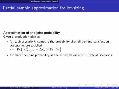
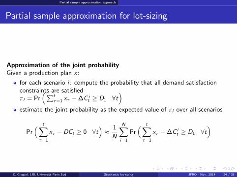
Approximation of the joint probabilityGiven a production plan x :
for each scenario i : compute the probability that all demand satisfactionconstraints are satisfiedπi = Pr
(∑tτ=1 xτ −∆C i
t ≥ D1 ∀t)
estimate the joint probability as the expected value of πi over all scenarios
Pr( t∑
τ=1
xτ − DCt ≥ 0 ∀t)≈ 1
N
N∑i=1
Pr( t∑
τ=1
xτ −∆C it ≥ D1 ∀t
)
C. Gicquel, LRI, Universite Paris Sud Stochastic lot-sizing JFRO - Nov. 2014 24 / 35
Partial sample approximation approach
Partial sample approximation for lot-sizing
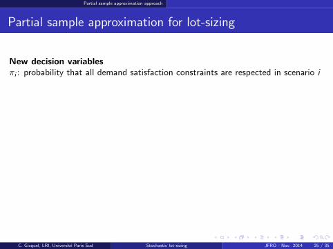
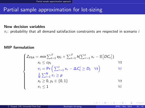
New decision variablesπi : probability that all demand satisfaction constraints are respected in scenario i
MIP formulation
ZPSA = min∑T
t=1 syt +∑T
t=1 h(∑t
τ=1 xτ − E[DCt
])
xt ≤ cyt ∀tπi = Pr
(∑tτ=1 xτ −∆C i
t ≥ D1 ∀t)
∀i1N
∑Ni=1 πi ≥ p
xt ≥ 0, yt ∈ {0, 1} ∀tπi ≤ 1 ∀i
C. Gicquel, LRI, Universite Paris Sud Stochastic lot-sizing JFRO - Nov. 2014 25 / 35
Partial sample approximation approach
Partial sample approximation for lot-sizing
New decision variablesπi : probability that all demand satisfaction constraints are respected in scenario i
MIP formulation
ZPSA = min∑T
t=1 syt +∑T
t=1 h(∑t
τ=1 xτ − E[DCt
])
xt ≤ cyt ∀tπi = Pr
(∑tτ=1 xτ −∆C i
t ≥ D1 ∀t)
∀i1N
∑Ni=1 πi ≥ p
xt ≥ 0, yt ∈ {0, 1} ∀tπi ≤ 1 ∀i
C. Gicquel, LRI, Universite Paris Sud Stochastic lot-sizing JFRO - Nov. 2014 25 / 35
Partial sample approximation approach
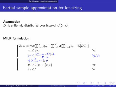
Partial sample approximation for lot-sizing
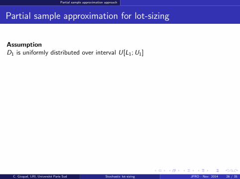
AssumptionD1 is uniformly distributed over interval U[L1;U1]
MILP formulation
ZPSA = min∑T
t=1 syt +∑T
t=1 h(∑t
τ=1 xτ − E[DCt
])
xt ≤ cyt ∀tπi ≤
∑tτ=1 xτ−∆C i
t−L1
U1−L1∀i ,∀t
1N
∑Ni=1 πi ≥ p
xt ≥ 0, yt ∈ {0, 1} ∀tπi ≤ 1 ∀i
C. Gicquel, LRI, Universite Paris Sud Stochastic lot-sizing JFRO - Nov. 2014 26 / 35
Partial sample approximation approach
Partial sample approximation for lot-sizing
AssumptionD1 is uniformly distributed over interval U[L1;U1]
MILP formulation
ZPSA = min∑T
t=1 syt +∑T
t=1 h(∑t
τ=1 xτ − E[DCt
])
xt ≤ cyt ∀tπi ≤
∑tτ=1 xτ−∆C i
t−L1
U1−L1∀i ,∀t
1N
∑Ni=1 πi ≥ p
xt ≥ 0, yt ∈ {0, 1} ∀tπi ≤ 1 ∀i
C. Gicquel, LRI, Universite Paris Sud Stochastic lot-sizing JFRO - Nov. 2014 26 / 35
Preliminary computational results
Plan
1 Deterministic lot-sizing problem
2 Stochastic lot-sizing problem
3 Sample approximation approach
4 Partial sample approximation approach
5 Preliminary computational results
6 Conclusion and perspectives
C. Gicquel, LRI, Universite Paris Sud Stochastic lot-sizing JFRO - Nov. 2014 27 / 35
Preliminary computational results
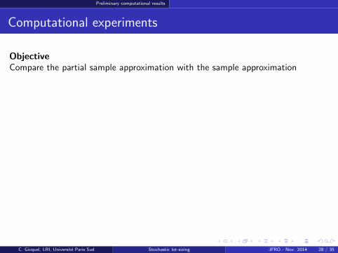
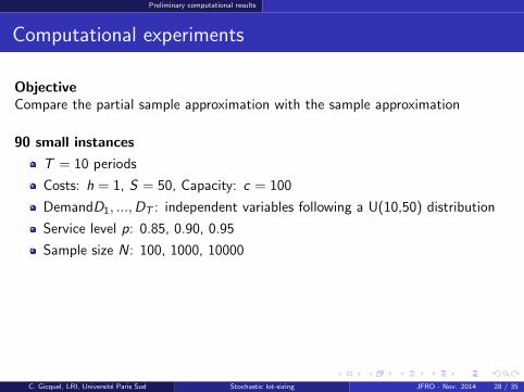
Computational experiments
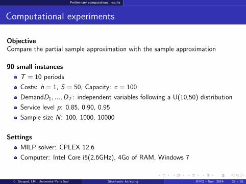
ObjectiveCompare the partial sample approximation with the sample approximation
90 small instances
T = 10 periods
Costs: h = 1, S = 50, Capacity: c = 100
DemandD1, ...,DT : independent variables following a U(10,50) distribution
Service level p: 0.85, 0.90, 0.95
Sample size N: 100, 1000, 10000
Settings
MILP solver: CPLEX 12.6
Computer: Intel Core i5(2.6GHz), 4Go of RAM, Windows 7
C. Gicquel, LRI, Universite Paris Sud Stochastic lot-sizing JFRO - Nov. 2014 28 / 35
Preliminary computational results
Computational experiments
ObjectiveCompare the partial sample approximation with the sample approximation
90 small instances
T = 10 periods
Costs: h = 1, S = 50, Capacity: c = 100
DemandD1, ...,DT : independent variables following a U(10,50) distribution
Service level p: 0.85, 0.90, 0.95
Sample size N: 100, 1000, 10000
Settings
MILP solver: CPLEX 12.6
Computer: Intel Core i5(2.6GHz), 4Go of RAM, Windows 7
C. Gicquel, LRI, Universite Paris Sud Stochastic lot-sizing JFRO - Nov. 2014 28 / 35

Preliminary computational results
Computational experiments
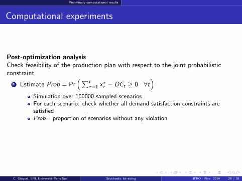
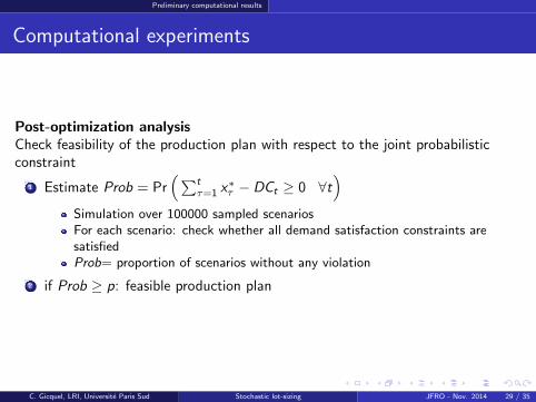
Post-optimization analysisCheck feasibility of the production plan with respect to the joint probabilisticconstraint
1 Estimate Prob = Pr(∑t
τ=1 x∗τ − DCt ≥ 0 ∀t
)Simulation over 100000 sampled scenariosFor each scenario: check whether all demand satisfaction constraints aresatisfiedProb= proportion of scenarios without any violation
2 if Prob ≥ p: feasible production plan
C. Gicquel, LRI, Universite Paris Sud Stochastic lot-sizing JFRO - Nov. 2014 29 / 35
Preliminary computational results
Computational experiments
Post-optimization analysisCheck feasibility of the production plan with respect to the joint probabilisticconstraint
1 Estimate Prob = Pr(∑t
τ=1 x∗τ − DCt ≥ 0 ∀t
)Simulation over 100000 sampled scenariosFor each scenario: check whether all demand satisfaction constraints aresatisfiedProb= proportion of scenarios without any violation
2 if Prob ≥ p: feasible production plan
C. Gicquel, LRI, Universite Paris Sud Stochastic lot-sizing JFRO - Nov. 2014 29 / 35
Preliminary computational results
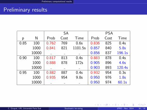
Preliminary results
SA PSAp N Prob Cost Time Prob Cost Time
0.85 100 0.762 769 0.6s 0.836 825 0.4s1000 0.841 821 1101.5s 0.857 840 5.8s
10000 0.856 837 196.1s0.90 100 0.817 813 0.4s 0.883 878 0.4s
1000 0.888 878 172s 0.905 896 4.6s10000 0.903 893 120.4s
0.95 100 0.882 887 0.4s 0.932 954 0.3s1000 0.935 954 9.8s 0.950 976 1.8s
10000 0.950 974 60.1s
C. Gicquel, LRI, Universite Paris Sud Stochastic lot-sizing JFRO - Nov. 2014 30 / 35
Conclusion and perspectives
Plan
1 Deterministic lot-sizing problem
2 Stochastic lot-sizing problem
3 Sample approximation approach
4 Partial sample approximation approach
5 Preliminary computational results
6 Conclusion and perspectives
C. Gicquel, LRI, Universite Paris Sud Stochastic lot-sizing JFRO - Nov. 2014 31 / 35

Conclusion and perspectives
Conclusion and perspectives
Conclusion
Single-item capacitated lot-sizing with stochastic demand
Joint chance-constrained programming formulation
New solution approach: partial sample approximation
Feasible solutions within reduced computation times
Perspectives
Confirm results on a larger set of instances
Extend to normally distributed demands
C. Gicquel, LRI, Universite Paris Sud Stochastic lot-sizing JFRO - Nov. 2014 32 / 35
Conclusion and perspectives
Conclusion and perspectives
Conclusion
Single-item capacitated lot-sizing with stochastic demand
Joint chance-constrained programming formulation
New solution approach: partial sample approximation
Feasible solutions within reduced computation times
Perspectives
Confirm results on a larger set of instances
Extend to normally distributed demands
C. Gicquel, LRI, Universite Paris Sud Stochastic lot-sizing JFRO - Nov. 2014 32 / 35
Conclusion and perspectives
Thank you for your attention !
C. Gicquel, LRI, Universite Paris Sud Stochastic lot-sizing JFRO - Nov. 2014 33 / 35