Step By Step Instructions for 2D NMR Experiments on the Bruker 300 MHz Spectrometer

(1) Use the drop down menu to create a new experiment/dataset for acquiring the 1D proton

spectra. The name of this data set should be used for the rest of the experiments. Be sure to

set the experiment number to 1.

(2) Go through the normal steps for acquiring the 1D proton spectra and acquire this spectra

(3) Ensure that the shims are sufficient for the resolution you would like in your 2D spectra.

If you are unhappy with the shims you can either manually shim or go through another auto-

shim process.

(4) Reference your proton spectra and then write down the value for the SR parameter.

Referencing can be done by clicking on the calibrate spectrum option in the NMR step by

step drop down menu. The SR parameter can be found in the ProcPars tab or by simply

typing SR in the command line and pressing enter.

(5) Examine your referenced spectra to determine the required sweep width (SW). By default

the proton SW is much larger than required and you will want to make sure that you use the

smallest possible SW in your 2D acquisition. Remember that the SW must contain all peaks

in the spectra in order to avoid folding. Make sure that you write down the value for the

SW as you will need this value later when setting up the 2D experiment.

(6) Center the rf transmitter in the middle of the required sweep width. MAKE SURE that you

are doing this after referencing your spectra. The rf transmitter can be centered by typing o1p

into the command line and pressing enter.This will cause a box to appear and you can enter

the frequency of the transmitter, in ppm, directly into this box. This value should be the

middle of your spectra. Make sure that you write down the value for 01p as this will be used

later when setting up the 2D experiment.

(7) If you are carrying out a hetero-nuclear 2D experiment, such as HSQC or HMBC, you must

repeat steps 1-6 for the carbon nucleus. Be sure to use the same name for your data set but

enter the experiment number as 2. You will also need to write down the sweep width (SW),

o1p, and SR values for the carbon experiment.

(8) Create a new data set using the NMR step by step drop down menu. Again, use the same

name for the experiment as you did in the previous steps but use a different experiment

number (ex. 3 or 4 or 5).

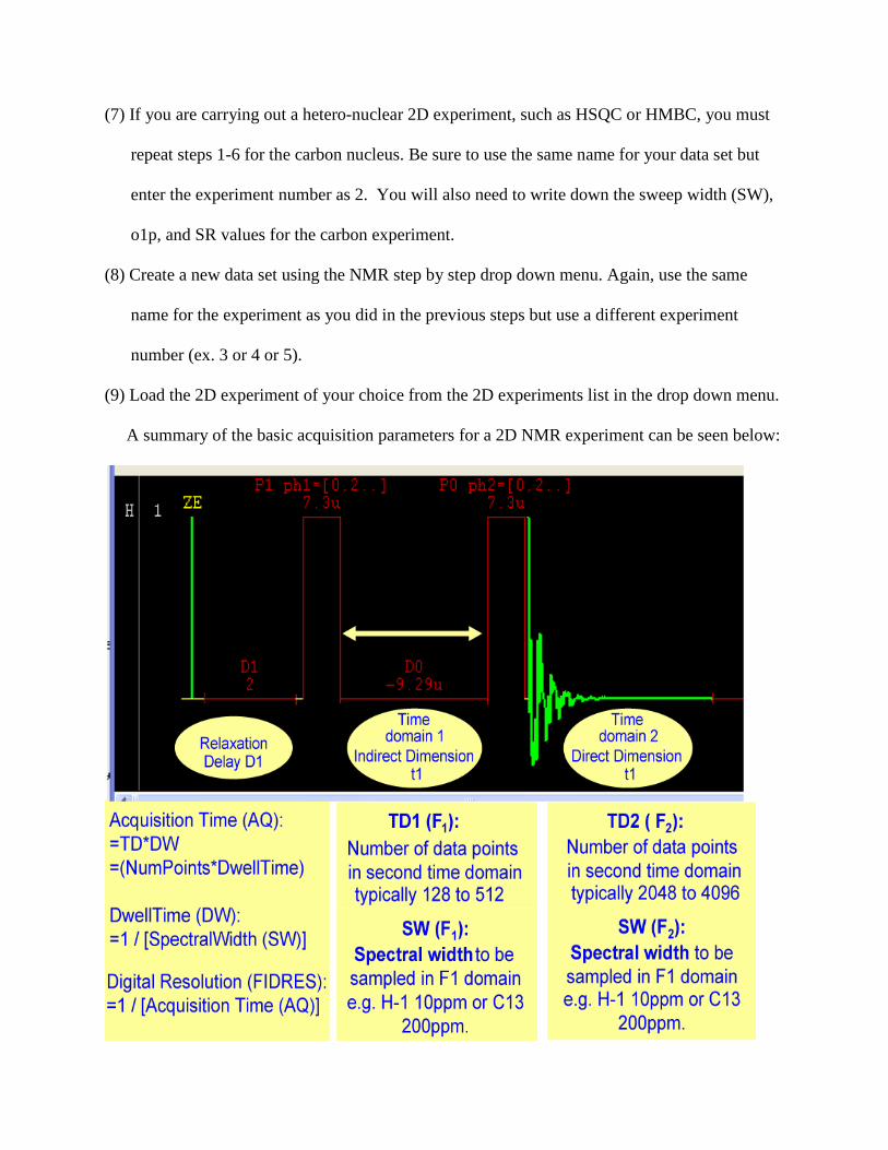
(9) Load the 2D experiment of your choice from the 2D experiments list in the drop down menu.

A summary of the basic acquisition parameters for a 2D NMR experiment can be seen below:

(10) Enter the sweep width for each dimension.

This can be done by clicking on the AcquPars tab and entering the SW for each nucleus into

the F2 and F1 columns. If you are carrying out a COSY experiment then the values for SW

in F1 and F2 should be equal to the SW value from your 1D proton experiment. If you are

carrying out an HSQC or HMBC then the value for SW in F2 and F1 should correspond to

the SW value you recorded earlier for the 1D proton and 1D carbon experiments,

respectively (see figure below).

(11) Center the RF transmitter in the middle of your sweep width for both dimensions. This can

be done by typing o1p into the command line and hitting enter. A box will appear and you

can enter the value for o1p recorded earlier. Repeat this step for o2p by typing o2p into the

command line and hitting enter. Note if you are running a COSY then the value of o1p and

o2p will be the same. If you are running a HSQC or HMBC then the value of o1p and o2p

correspond to the o1p value from the 1D proton and 1D carbon experiments, respectively

(see figure below).

(12) Optimize the digital resolution of your direct and indirect dimensions/FID.

Remember that the digital resolutions (FIDRES) is equal to 1/[acquisition time (AQ)] and a

smaller number for the digital resolution corresponds to better resolution. This corresponds

to increasing the acquisition time (AQ). Recall that the acquisition time is equal to the

number of points (TD) multiplied by the dwell time (DW). Since the dwell time is equal to

1/[sweep width (SW)], and the SW value has been determined, the only way to enhance the

digital resolution is to increase the number of points (TD). NOTE: The number or points

(TD) in the indirect dimension (F1) is more commonly referred to as the number of

Increments (see figure below).

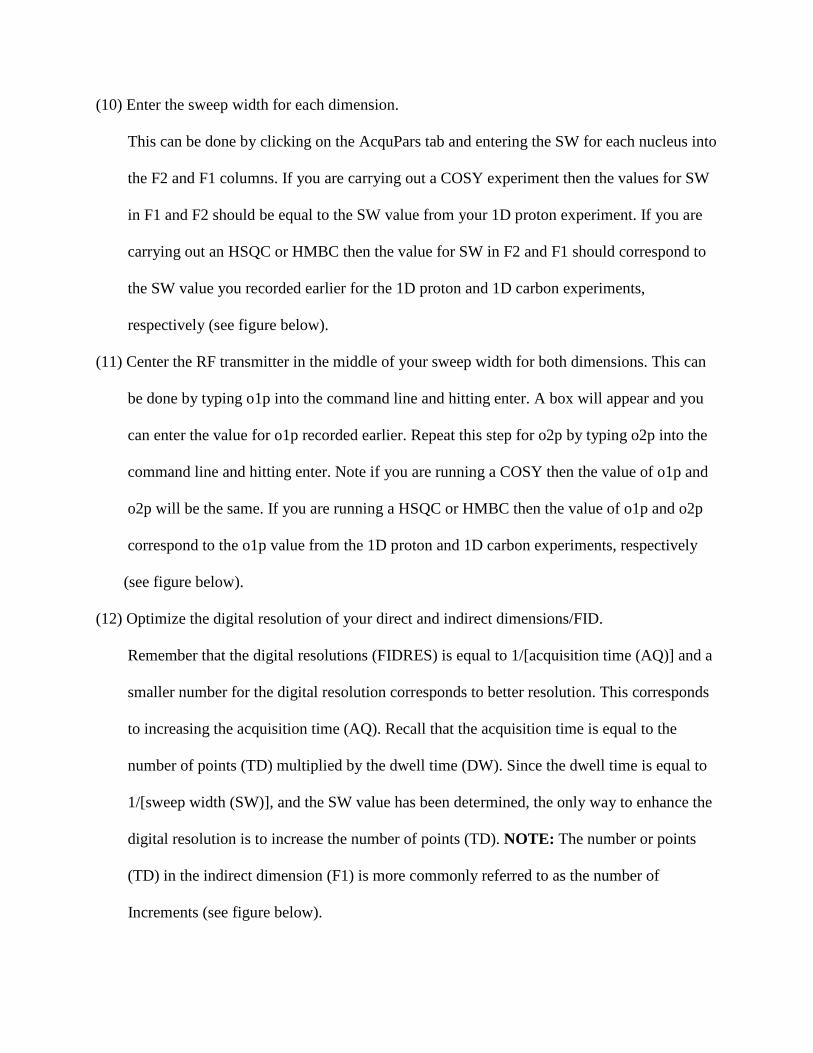
(13) Set the number or scans (NS) to be carried out.

In the step 12 you optimized the digital resolution based on the acquisition parameters. In

this step you will vary the number of scans (NS) for each increment in order to

increase/optimize the signal to noise ratio for the experiment. Remember that a high quality

HSQC and HMBC will have a balance of both good digital resolution and a high signal to

noise ratio (see figure below).

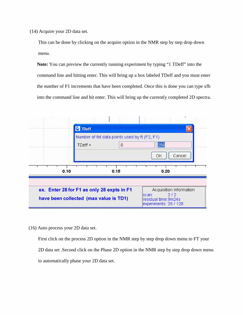
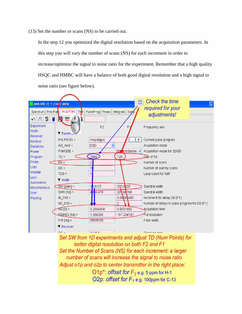
(14) Acquire your 2D data set.

This can be done by clicking on the acquire option in the NMR step by step drop down

menu.

Note: You can preview the currently running experiment by typing “1 TDeff” into the

command line and hitting enter. This will bring up a box labeled TDeff and you must enter

the number of F1 increments that have been completed. Once this is done you can type xfb

into the command line and hit enter. This will bring up the currently completed 2D spectra.

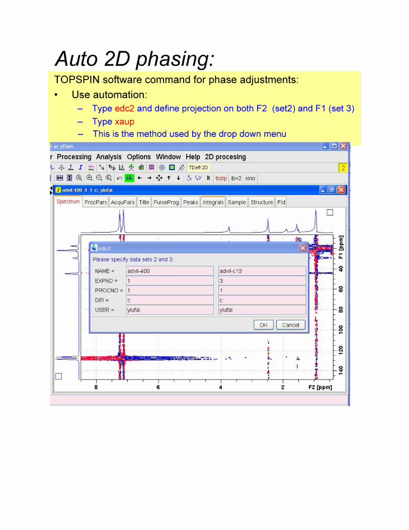
(16) Auto process your 2D data set.

First click on the process 2D option in the NMR step by step drop down menu to FT your

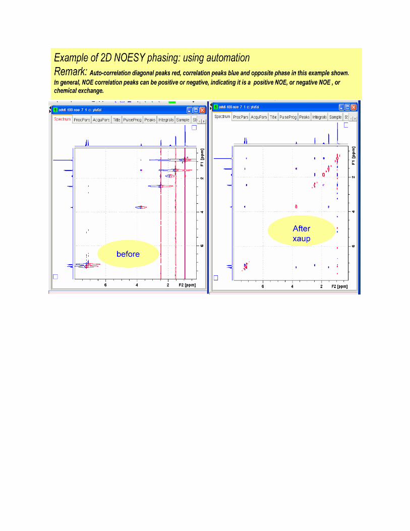
2D data set .Second click on the Phase 2D option in the NMR step by step drop down menu

to automatically phase your 2D data set.

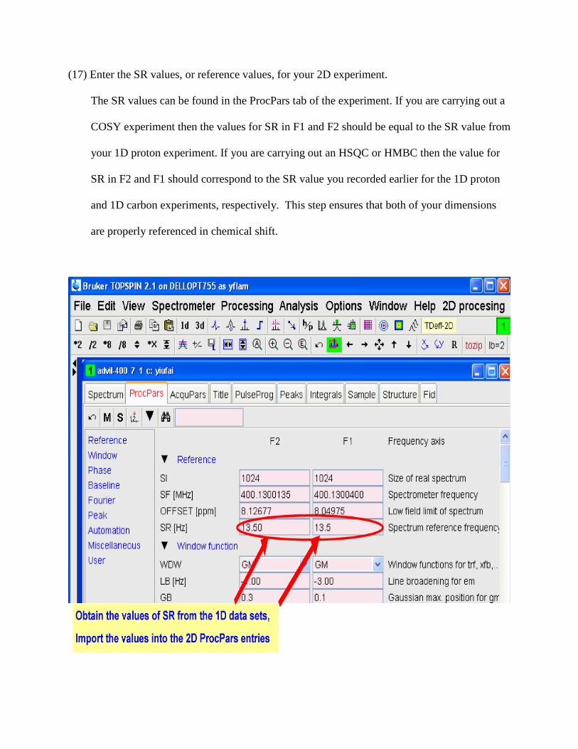
(17) Enter the SR values, or reference values, for your 2D experiment.

The SR values can be found in the ProcPars tab of the experiment. If you are carrying out a

COSY experiment then the values for SR in F1 and F2 should be equal to the SR value from

your 1D proton experiment. If you are carrying out an HSQC or HMBC then the value for

SR in F2 and F1 should correspond to the SR value you recorded earlier for the 1D proton

and 1D carbon experiments, respectively. This step ensures that both of your dimensions

are properly referenced in chemical shift.

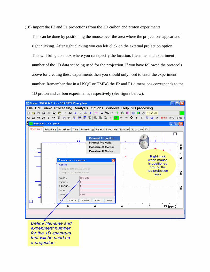
(18) Import the F2 and F1 projections from the 1D carbon and proton experiments.

This can be done by positioning the mouse over the area where the projections appear and

right clicking. After right clicking you can left click on the external projection option.

This will bring up a box where you can specify the location, filename, and experiment

number of the 1D data set being used for the projection. If you have followed the protocols

above for creating these experiments then you should only need to enter the experiment

number. Remember that in a HSQC or HMBC the F2 and F1 dimensions corresponds to the

1D proton and carbon experiments, respectively (See figure below).

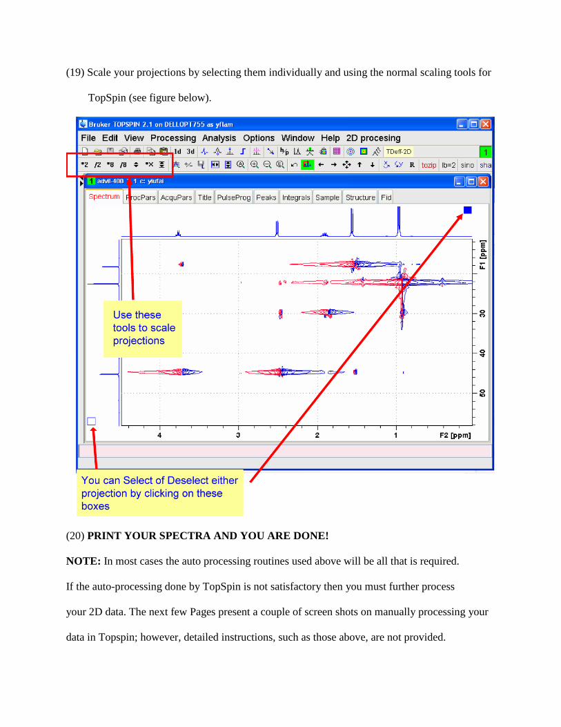
(19) Scale your projections by selecting them individually and using the normal scaling tools for

TopSpin (see figure below).

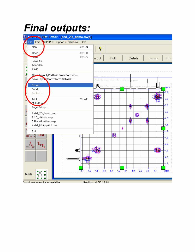
(20) PRINT YOUR SPECTRA AND YOU ARE DONE!

NOTE: In most cases the auto processing routines used above will be all that is required.

If the auto-processing done by TopSpin is not satisfactory then you must further process

your 2D data. The next few Pages present a couple of screen shots on manually processing your

data in Topspin; however, detailed instructions, such as those above, are not provided.

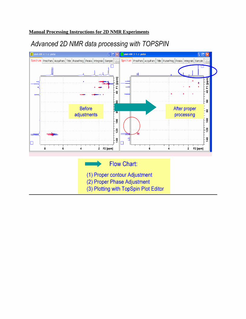
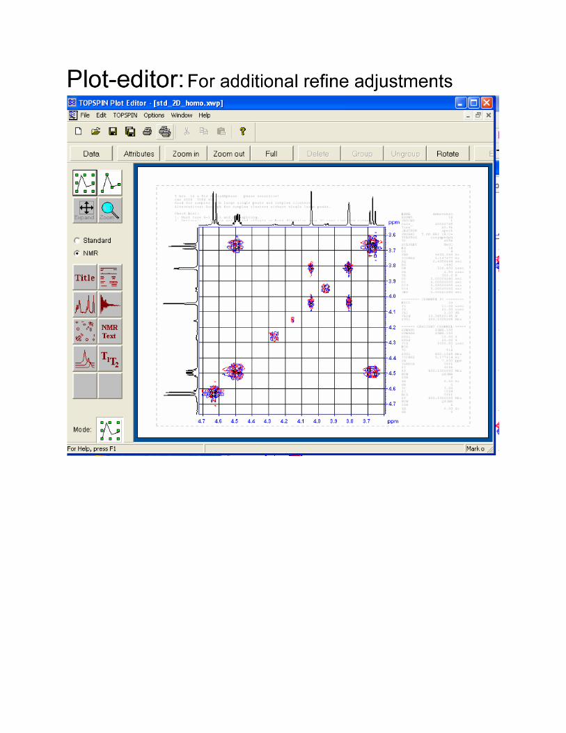
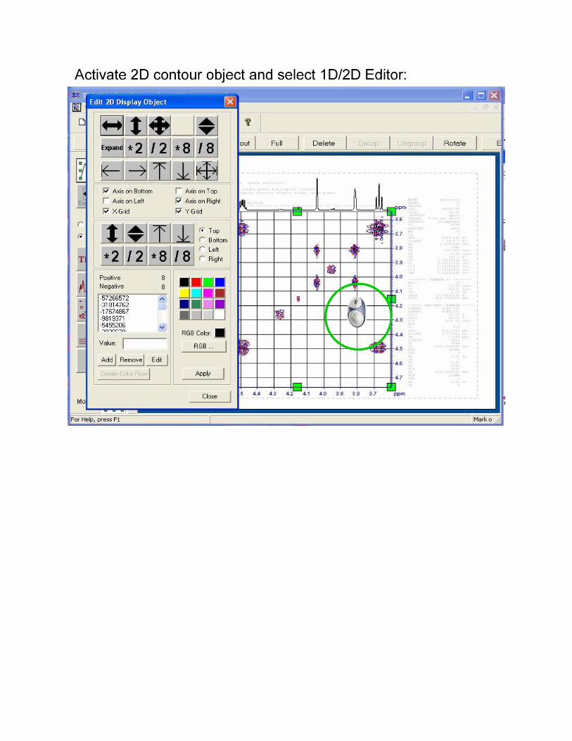
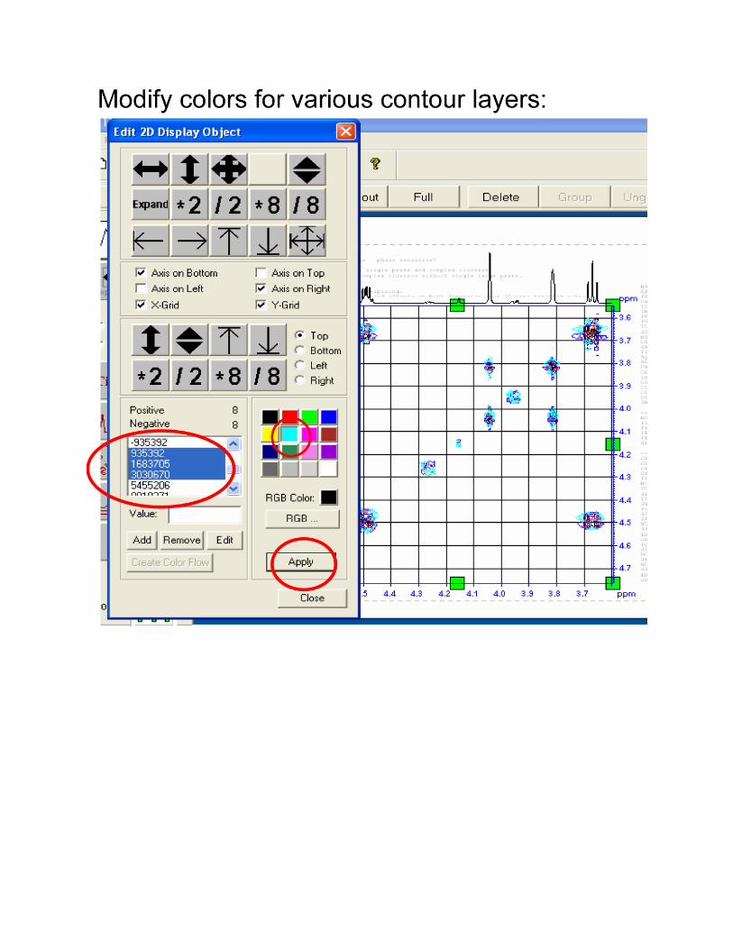
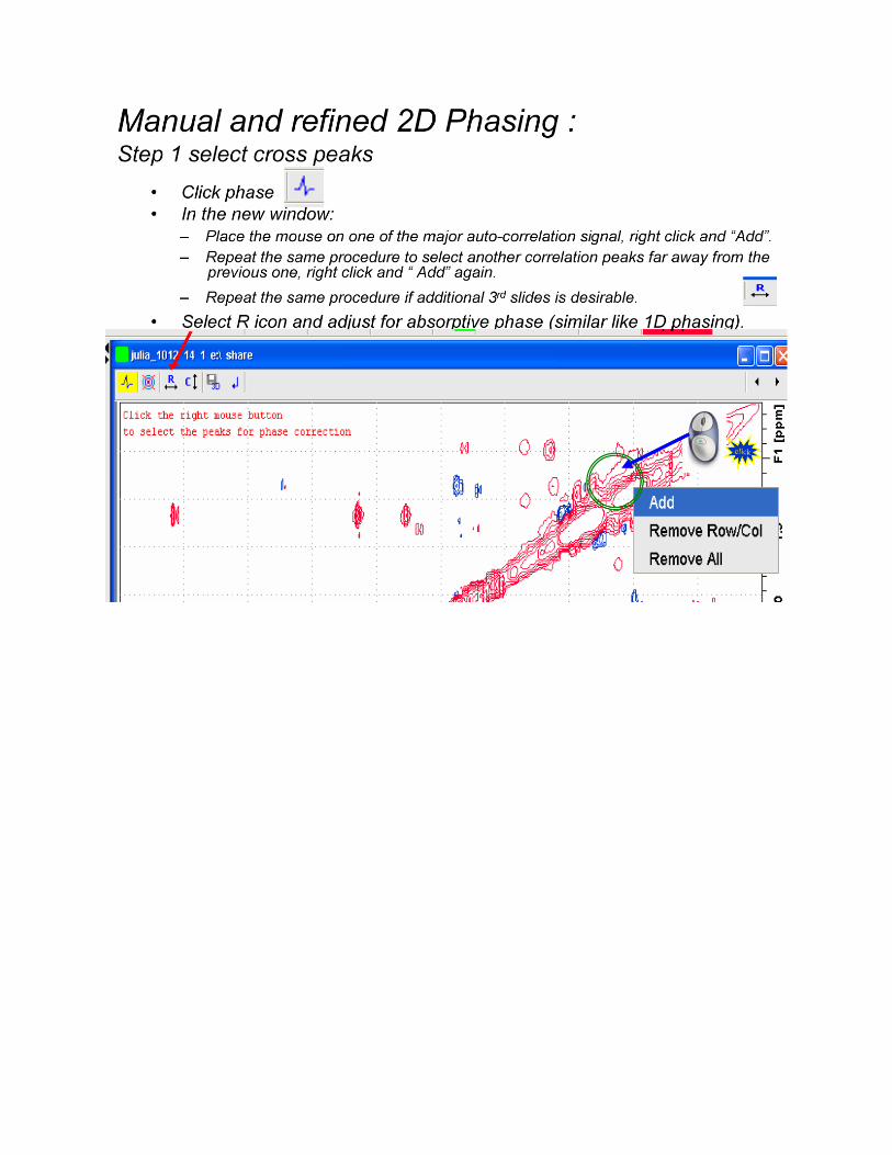
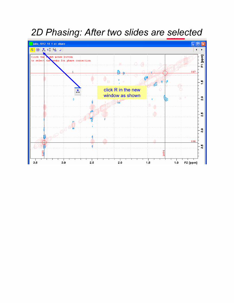
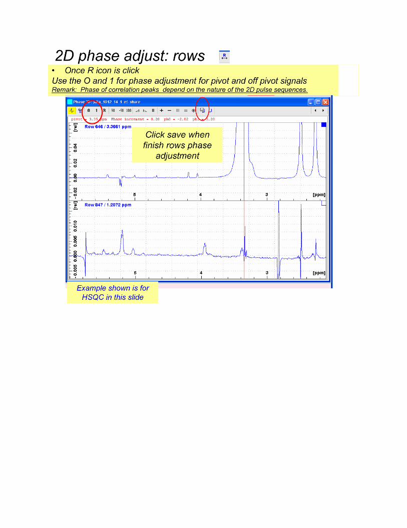
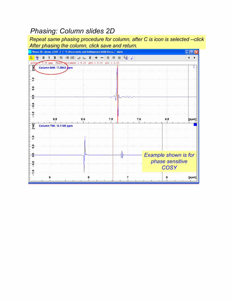
Manual Processing Instructions for 2D NMR Experiments

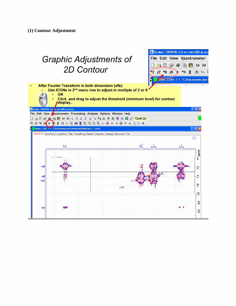
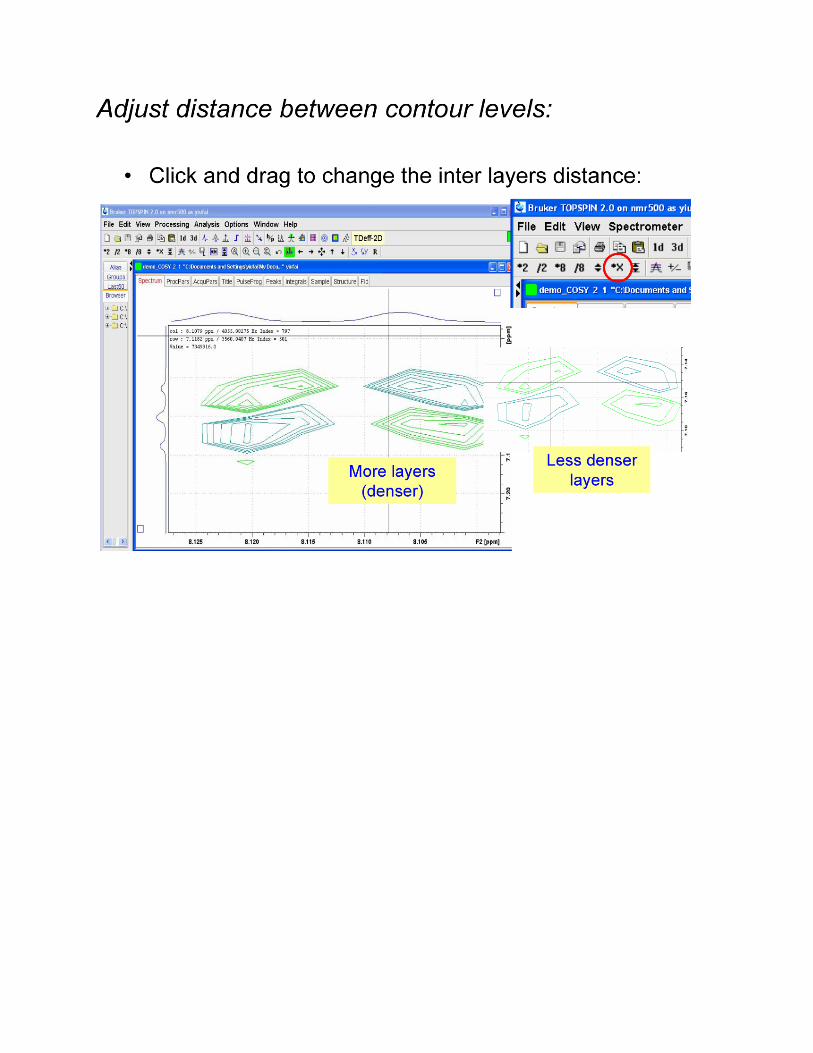
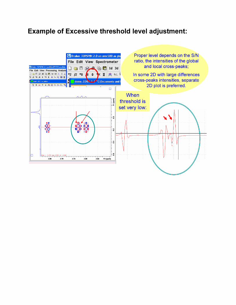
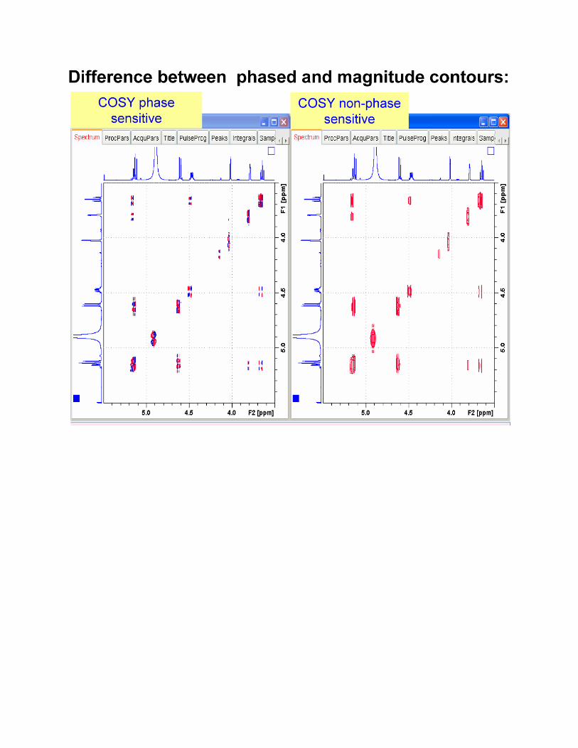
(1) Contour Adjustment

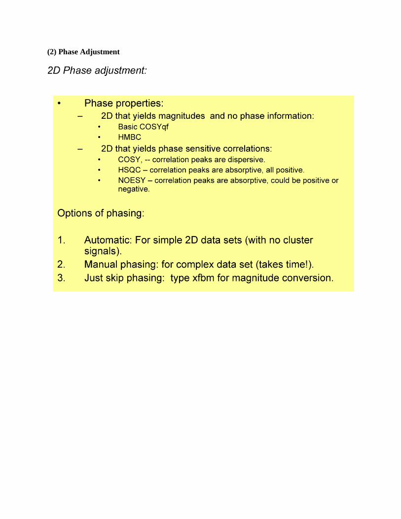
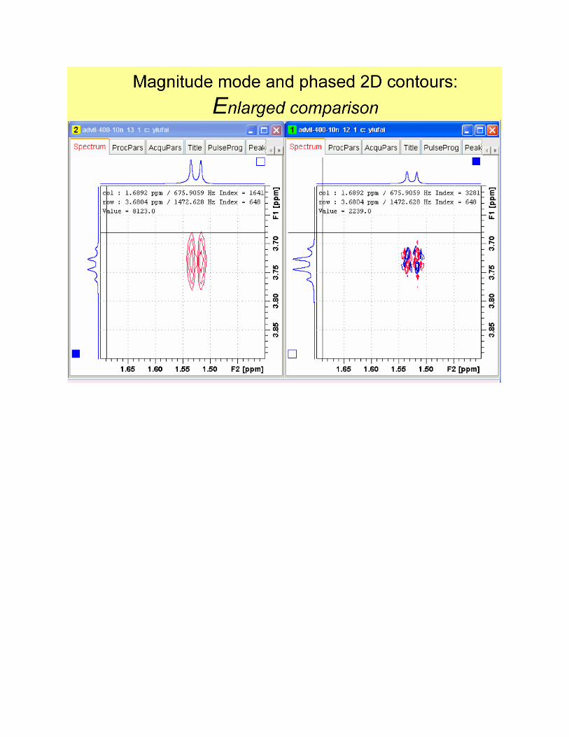
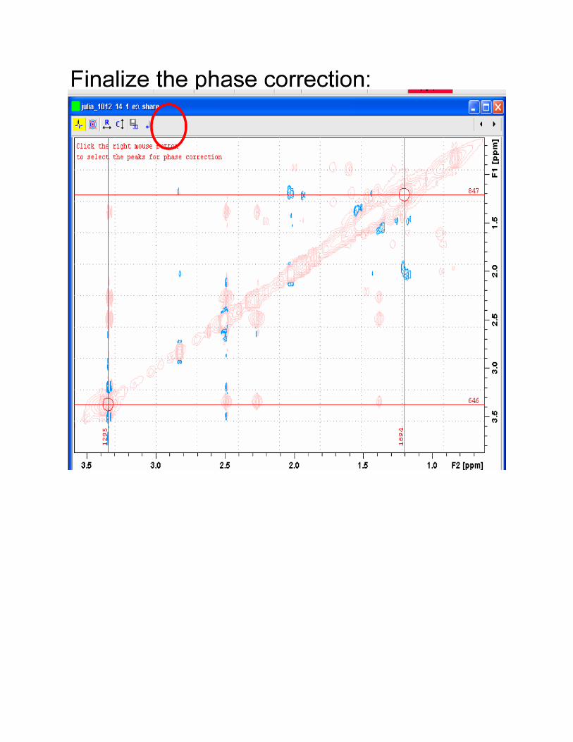
(2) Phase Adjustment

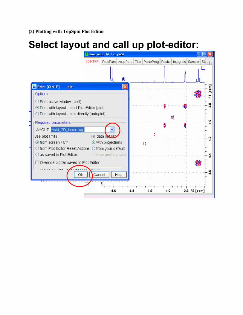
(3) Plotting with TopSpin Plot Editor