statsbomb data in r accessing and working with
TRANSCRIPT
Accessing and Working WithStatsBomb Data In R

What is R and Why Use It?
R is a programming language that is useful for managing large datasets. It is especially useful in the world of football data, as it allows us to manipulate that data to various ends. Such as creating metrics out of the data and visualising it.
R itself can be downloaded here:
https://cran.r-project.org/mirrors.html
We at StatsBomb use R regularly (amongst other coding languages) in day-to-day work, particularly within our analysis department. Spreadsheets are a viable route when you’re just starting out, but eventually the datasets become too big and unwieldy, performing nuanced dissection of them becomes too complicated.
Once you’ve gotten over the learning curve, R is ideal for parsing data and working with it however you like in a fast manner.
What Is R and Why Use It?
The base version of R is a somewhat cumbersome piece of software. This has lead to the creation of many different ‘IDE’s (integrated development environment). These are wrappers around the initial R install that make most tasks within R easier and more manageable for the end user. The most popular of these is RStudio:
https://www.rstudio.com/products/rstudio/
It is recommended that you install RStudio (or any similar IDE that you find and prefer) as most users do. It will make working with StatsBomb’s data a cleaner, simpler process.
RStudio
Opening a New R ‘Project’
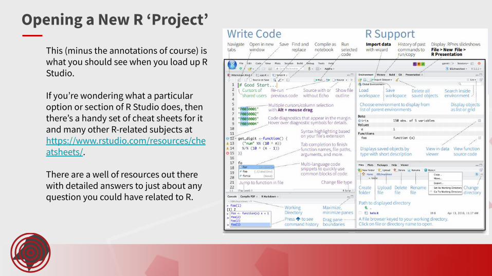
This (minus the annotations of course) is what you should see when you load up R Studio.
If you’re wondering what a particular option or section of R Studio does, then there’s a handy set of cheat sheets for it and many other R-related subjects at https://www.rstudio.com/resources/cheatsheets/.
There are a well of resources out there with detailed answers to just about any question you could have related to R.
Packages & ‘StatsBombR’
‘Packages’ are downloadable bundles of functions that make tasks easier. Most packages are installed by running install.packages(‘PackageNameHere’). However, if the package comes via Github we use the devtools package to install it (this includes StatsBombR, which we will walk through installing on the next page).
The main packages we will focus on here and which need installing are:
‘tidyverse’: tidyverse contains a whole host of other packages (such as dplyr and magrittr) that are useful for manipulating data. install.packages(“tidyverse”)
‘devtools’: Most packages are hosted on CRAN. However there are also countless useful ones hosted on Github. Devtools allows for downloading of packages directly from Github. install.packages(“devtools”)
‘ggplot2’: The most popular package for visualising data within R. It is contained within tidyverse.
‘StatsBombR’: This is StatsBomb’s own package for parsing our data.
Once a package is installed it can be loaded into R by running library(PackageNameHere). You should load all of these at the start of any session.
What is an R ‘Package’?
StatsBomb’s former data scientist Derrick Yam created ‘StatsBombR’, an R package dedicated to making using StatBomb’s data in R much easier. It can be found on Github at the following link, along with much more information on its uses. There are lots of helpful functions within it that you should get to know.
https://github.com/statsbomb/StatsBombR
To install the package in R, you’ll need to install the ‘Devtools’ package, which can be done by running the following line of code:
install.packages("devtools")
Then, to install StatsBombR itself, run:
devtools::install_github("statsbomb/StatsBombR")
What is ‘StatsBombR’ and how to Install it?
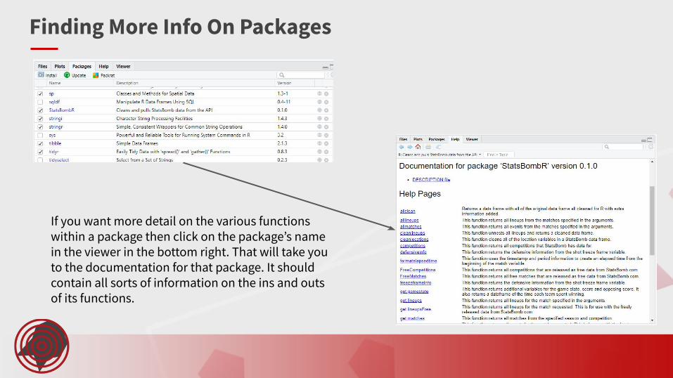
Finding More Info On Packages
If you want more detail on the various functions within a package then click on the package’s name in the viewer in the bottom right. That will take you to the documentation for that package. It should contain all sorts of information on the ins and outs of its functions.
Pulling in StatsBomb Data
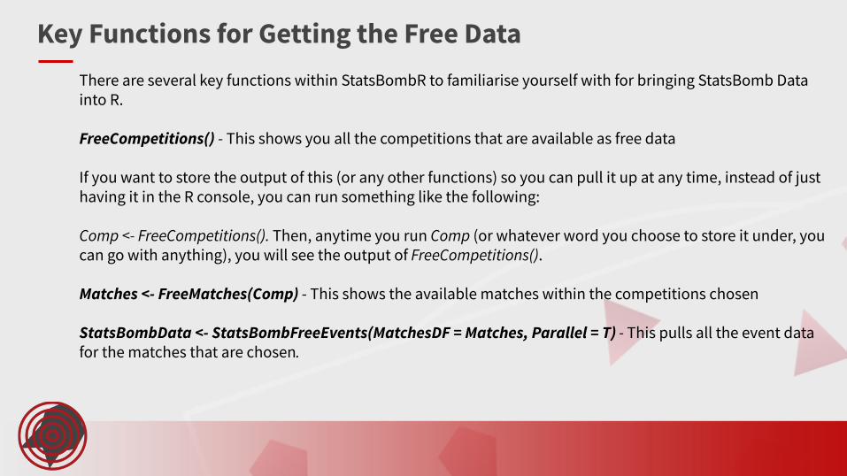
There are several key functions within StatsBombR to familiarise yourself with for bringing StatsBomb Data into R.
FreeCompetitions() - This shows you all the competitions that are available as free data
If you want to store the output of this (or any other functions) so you can pull it up at any time, instead of just having it in the R console, you can run something like the following:
Comp <- FreeCompetitions(). Then, anytime you run Comp (or whatever word you choose to store it under, you can go with anything), you will see the output of FreeCompetitions().
Matches <- FreeMatches(Comp) - This shows the available matches within the competitions chosen
StatsBombData <- StatsBombFreeEvents(MatchesDF = Matches, Parallel = T) - This pulls all the event data for the matches that are chosen.
Key Functions for Getting the Free Data
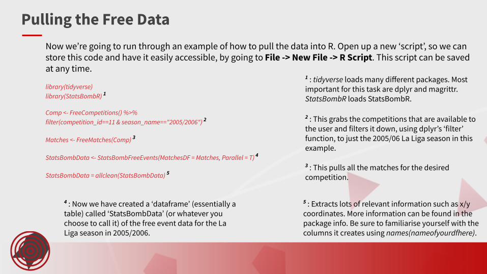
Now we’re going to run through an example of how to pull the data into R. Open up a new ‘script’, so we can store this code and have it easily accessible, by going to File -> New File -> R Script. This script can be saved at any time.
Pulling the Free Data
library(tidyverse) library(StatsBombR) 1
Comp <- FreeCompetitions() %>% filter(competition_id==11 & season_name=="2005/2006") 2
Matches <- FreeMatches(Comp) 3
StatsBombData <- StatsBombFreeEvents(MatchesDF = Matches, Parallel = T) 4
StatsBombData = allclean(StatsBombData) 5
1 : tidyverse loads many different packages. Most important for this task are dplyr and magrittr. StatsBombR loads StatsBombR.
2 : This grabs the competitions that are available to the user and filters it down, using dplyr’s ‘filter’ function, to just the 2005/06 La Liga season in this example.
3 : This pulls all the matches for the desired competition.
4 : Now we have created a ‘dataframe’ (essentially a table) called ‘StatsBombData’ (or whatever you choose to call it) of the free event data for the La Liga season in 2005/2006.
5 : Extracts lots of relevant information such as x/y coordinates. More information can be found in the package info. Be sure to familiarise yourself with the columns it creates using names(nameofyourdfhere).
Working With the Data
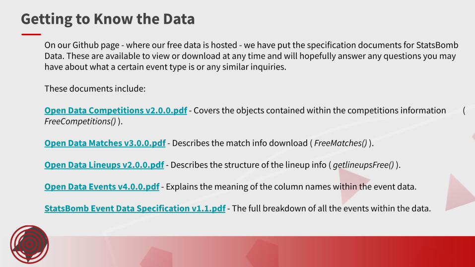
On our Github page - where our free data is hosted - we have put the specification documents for StatsBomb Data. These are available to view or download at any time and will hopefully answer any questions you may have about what a certain event type is or any similar inquiries.
These documents include:
Open Data Competitions v2.0.0.pdf - Covers the objects contained within the competitions information ( FreeCompetitions() ).
Open Data Matches v3.0.0.pdf - Describes the match info download ( FreeMatches() ).
Open Data Lineups v2.0.0.pdf - Describes the structure of the lineup info ( getlineupsFree() ).
Open Data Events v4.0.0.pdf - Explains the meaning of the column names within the event data.
StatsBomb Event Data Specification v1.1.pdf - The full breakdown of all the events within the data.
Getting to Know the Data
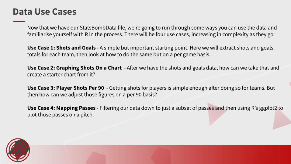
Now that we have our StatsBombData file, we’re going to run through some ways you can use the data and familiarise yourself with R in the process. There will be four use cases, increasing in complexity as they go:
Use Case 1: Shots and Goals - A simple but important starting point. Here we will extract shots and goals totals for each team, then look at how to do the same but on a per game basis.
Use Case 2: Graphing Shots On a Chart - After we have the shots and goals data, how can we take that and create a starter chart from it?
Use Case 3: Player Shots Per 90 - Getting shots for players is simple enough after doing so for teams. But then how can we adjust those figures on a per 90 basis?
Use Case 4: Mapping Passes - Filtering our data down to just a subset of passes and then using R’s ggplot2 to plot those passes on a pitch.
Data Use Cases
shots_goals = StatsBombData %>%
group_by(team.name) %>% 1
summarise(shots = sum(type.name=="Shot", na.rm = TRUE),
goals = sum(shot.outcome.name=="Goal", na.rm = TRUE)) 2
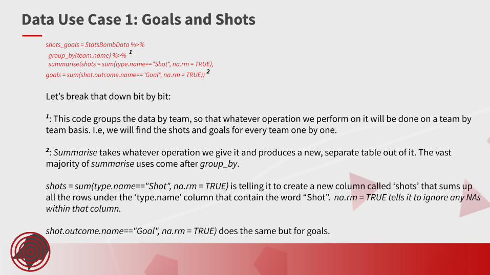
Let’s break that down bit by bit:
1: This code groups the data by team, so that whatever operation we perform on it will be done on a team by team basis. I.e, we will find the shots and goals for every team one by one.
2: Summarise takes whatever operation we give it and produces a new, separate table out of it. The vast majority of summarise uses come after group_by.
shots = sum(type.name=="Shot", na.rm = TRUE) is telling it to create a new column called ‘shots’ that sums up all the rows under the ‘type.name’ column that contain the word “Shot”. na.rm = TRUE tells it to ignore any NAs within that column.
shot.outcome.name=="Goal", na.rm = TRUE) does the same but for goals.
Data Use Case 1: Goals and Shots
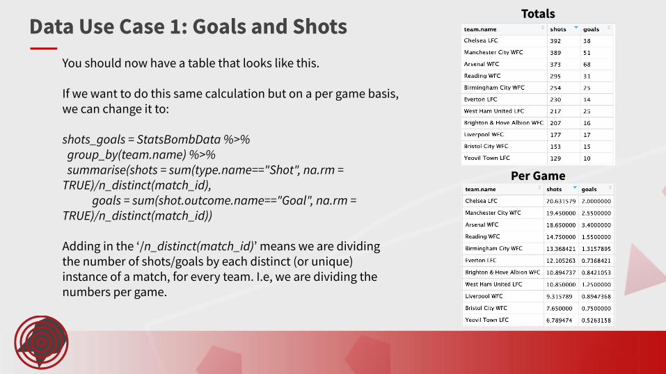
You should now have a table that looks like this.
If we want to do this same calculation but on a per game basis, we can change it to:
shots_goals = StatsBombData %>% group_by(team.name) %>% summarise(shots = sum(type.name=="Shot", na.rm = TRUE)/n_distinct(match_id), goals = sum(shot.outcome.name=="Goal", na.rm = TRUE)/n_distinct(match_id))
Adding in the ‘/n_distinct(match_id)’ means we are dividing the number of shots/goals by each distinct (or unique) instance of a match, for every team. I.e, we are dividing the numbers per game.
Data Use Case 1: Goals and Shots Totals
Per Game
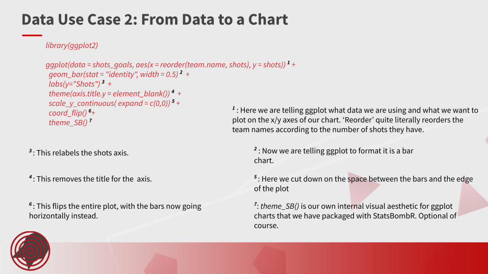
library(ggplot2)
ggplot(data = shots_goals, aes(x = reorder(team.name, shots), y = shots)) 1 + geom_bar(stat = "identity", width = 0.5) 2 + labs(y="Shots") 3 + theme(axis.title.y = element_blank()) 4 + scale_y_continuous( expand = c(0,0)) 5 + coord_flip() 6+ theme_SB() 7
Data Use Case 2: From Data to a Chart
1 : Here we are telling ggplot what data we are using and what we want to plot on the x/y axes of our chart. ‘Reorder’ quite literally reorders the team names according to the number of shots they have.
2 : Now we are telling ggplot to format it is a bar chart.
3 : This relabels the shots axis.
4 : This removes the title for the axis. 5 : Here we cut down on the space between the bars and the edge of the plot
6 : This flips the entire plot, with the bars now going horizontally instead.
7: theme_SB() is our own internal visual aesthetic for ggplot charts that we have packaged with StatsBombR. Optional of course.
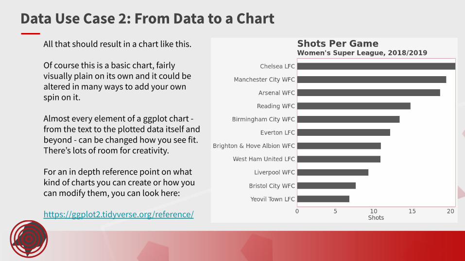
Data Use Case 2: From Data to a ChartAll that should result in a chart like this.
Of course this is a basic chart, fairly visually plain on its own and it could be altered in many ways to add your own spin on it.
Almost every element of a ggplot chart - from the text to the plotted data itself and beyond - can be changed how you see fit. There’s lots of room for creativity.
For an in depth reference point on what kind of charts you can create or how you can modify them, you can look here:
https://ggplot2.tidyverse.org/reference/
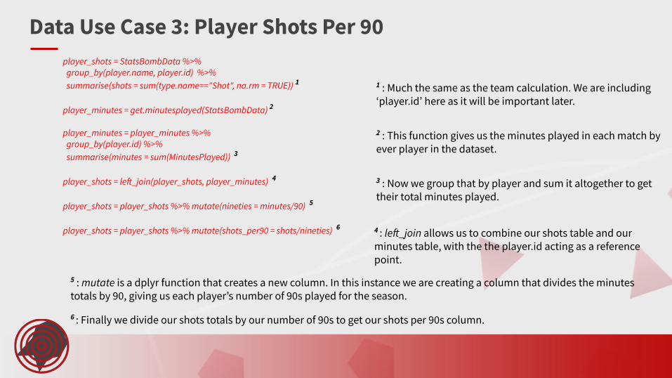
Data Use Case 3: Player Shots Per 90player_shots = StatsBombData %>% group_by(player.name, player.id) %>% summarise(shots = sum(type.name=="Shot", na.rm = TRUE)) 1
player_minutes = get.minutesplayed(StatsBombData) 2
player_minutes = player_minutes %>% group_by(player.id) %>% summarise(minutes = sum(MinutesPlayed)) 3
player_shots = left_join(player_shots, player_minutes) 4
player_shots = player_shots %>% mutate(nineties = minutes/90) 5
player_shots = player_shots %>% mutate(shots_per90 = shots/nineties) 6
1 : Much the same as the team calculation. We are including ‘player.id’ here as it will be important later.
2 : This function gives us the minutes played in each match by ever player in the dataset.
3 : Now we group that by player and sum it altogether to get their total minutes played.
4 : left_join allows us to combine our shots table and our minutes table, with the the player.id acting as a reference point.
5 : mutate is a dplyr function that creates a new column. In this instance we are creating a column that divides the minutes totals by 90, giving us each player’s number of 90s played for the season.
6 : Finally we divide our shots totals by our number of 90s to get our shots per 90s column.
Data Use Case 3: Player Shots Per 90
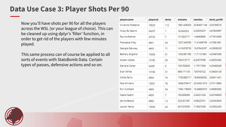
Now you’ll have shots per 90 for all the players across the WSL (or your league of choice). This can be cleaned up using dplyr’s ‘filter’ function, in order to get rid of the players with few minutes played.
This same process can of course be applied to all sorts of events with StatsBomb Data. Certain types of passes, defensive actions and so on.
Data Use Case 4: Plotting PassesFinally, we’re going to look at plotting a player’s passes on a pitch. For this we of course need some sort of pitch visualization. You might want to create your own once you become more familiar with ggplot and using it for more complex purposes (there will be a flexible version that we use later in this presentation). However, handily, there are several pre-made solutions out there.
The one we’ll be using here comes courtesy of FC rStats. A twitter user who has put together various helpful, public R packages for parsing football data. The package is called ‘SBPitch’ and it does exactly what it says on the tin. There will be further options in the ‘Other Useful Packages’ at the end of this document. First let’s get it installed with the following code:
devtools::install_github("FCrSTATS/SBpitch")
We’re going to plot Messi’s completed passes into the box for the 2005/2006 La Liga season. Plotting all of his passes would get messy of course, so this is a clearer subset. Make sure you’ve used the functions previously discussed to pull that data.

Data Use Case 4: Plotting Passeslibrary(SBpitch)
passes = messidata %>% filter(type.name=="Pass" & is.na(pass.outcome.name) & player.id==5503) 1 %>% filter(pass.end_location.x>=102 & pass.end_location.y<=62 & pass.end_location.y>=18) 2
create_Pitch() + geom_segment(data = passes, aes(x = location.x, y = location.y, xend = pass.end_location.x, yend = pass.end_location.y), lineend = "round", size = 0.6, arrow = arrow(length = unit(0.08, "inches"))) 3 + labs(title = "Lionel Messi, Completed Box Passes", subtitle = "La Liga, 2005/2006") 4 + scale_y_reverse()5 + coord_fixed(ratio = 105/100) 6
1 : Pull some of the Messi data of your choice and call it ‘messidata’ for us to work with here. Then we can filter to Messi’s passes. is.na(pass.outcome.name) filters to only completed passes.2 : Filtering to passes within the box. The coordinates for pitch markings in SBD can be found in our event spec.
3 : This creates an arrow from one point (location.x/y, the start part of the pass) to an end point (pass.end_location.x/y, the end of the pass). Lineend, size and length are are all customization options for the arrow.
4 : Creates a title and a subtitle for the plot. You can also add captions using caption =, along with other options.
6 : Fixes the plot to a certain aspect ratio of your choice, so it doesn’t look stretched.
5 : Reverses the y axis. Otherwise the data would be plotted on the wrong side of the pitch.
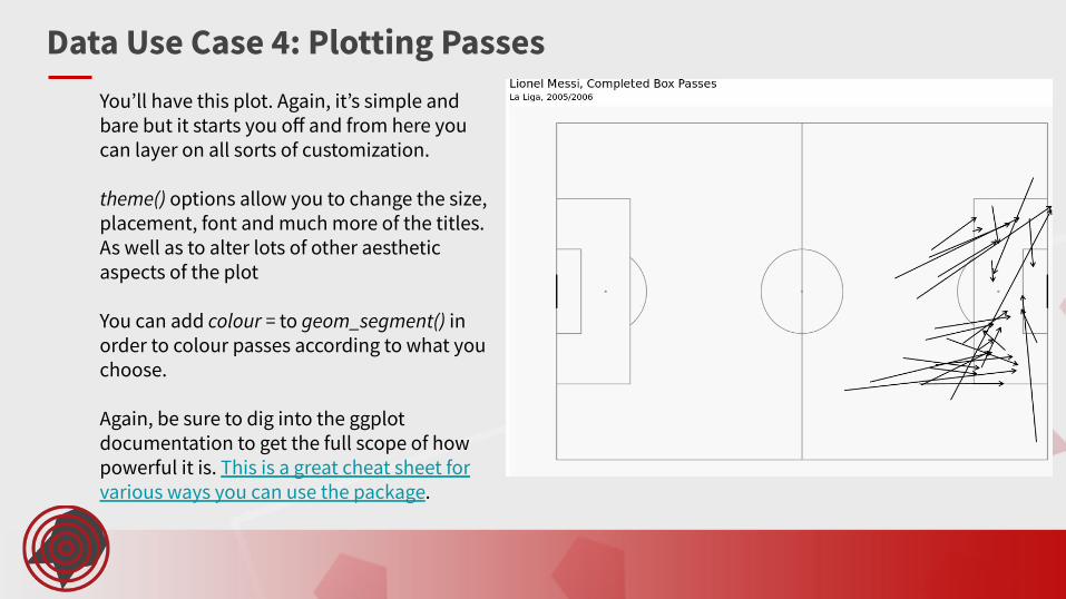
Data Use Case 4: Plotting PassesYou’ll have this plot. Again, it’s simple and bare but it starts you off and from here you can layer on all sorts of customization.
theme() options allow you to change the size, placement, font and much more of the titles. As well as to alter lots of other aesthetic aspects of the plot
You can add colour = to geom_segment() in order to colour passes according to what you choose.
Again, be sure to dig into the ggplot documentation to get the full scope of how powerful it is. This is a great cheat sheet for various ways you can use the package.
Useful StatsBombR FunctionsThere all sorts of functions within StatsBombR for different purposes. You can find them all here, deeper into the github page. Not all functions are related to the free data. Some are only accessible for customers via our API. Here’s a quick rundown of some you may find useful:
allclean() - Mentioned previously but to elucidate: this extrapolates lots of new, helpful columns from the pre existing columns. For example, it takes the location column and splits it up into separate x/y columns. It also extracts freeze frame data and goalkeeper information. Make sure to use.
get.playerfootedness() - Gives you a player’s assumed preferred foot using our pass footedness data.
get.opposingteam() - Returns an opposing team column for each team in each match.
get.gamestate() - Returns information for how much time each team spent in various game states (winning/drawing/losing) for each match.
annotate_pitchSB() - Our own solution for plotting a pitch with ggplot.
Other Useful Packages
The community around R is packed with packages that fulfill all sorts of needs. Chances are that, if you’re looking to do something in R or fix some sort of issue, there’s a package out there for it. There are far too many to name but here’s a brief selection of some that may be relevant to working with StatsBomb Data:
Ben Torvaney, ggsoccer - A package that contains an alternative for plotting a pitch with SB Data.
Joe Gallagher, soccermatics - Also offers an option for pitch plotting along with other useful shortcuts for creating heatmaps and so on.
ggrepel - Useful for when you’re having issues with overlapping labels on a chart.
gganimate - If you ever feel like getting more elaborate with your graphics, this gives you a simple way to create animated ones within R and ggplot.