statistics in psychology using r and spss (rasch/statistics in psychology using r and spss) ||...
TRANSCRIPT
P1: OTA/XYZ P2: ABCJWST094-c11 JWST094-Rasch September 22, 2011 16:25 Printer Name: Yet to Come
11
Regression and correlation
In this chapter we polarize deterministic relationships and dependencies on the one sideand stochastic relationships of two characters on the other side – thereby stochastic meansdependent on chance. Within the field of psychology only the latter relationships are ofinterest. We will deal at first with the graphical representation of corresponding observationpairs as a scatter plot. We will focus mainly on the linear regression function, which graspsthe relationship of two characters, modeled by two random variables. Then we will considerseveral correlation coefficients, which quantify the strength of relationship. Depending onthe scale type of the characters of interest, different coefficients become relevant. In additionto (point) estimators for the corresponding parameters, this chapter particularly deals withhypothesis testing concerning these parameters.
11.1 Introduction
The term ‘relationship’ can be explained by means of its colloquial sense. We know fromeveryday life, for instance, phrases and statements of the following type: ‘Children’s behavioris related to parents’ behavior’, ‘Learning effort and success in exams are related’, ‘Birth-rateand calendar month are related’, and so on.
Bachelor Example 11.1 Type and strength of the relationship between the ages of themother and father of last-born children is to be determined
From everyday life experience, as well as for obvious reasons, ages of bothparents are related. Although there are some extreme cases, for example a 40-year-old mother together with a 25-year-old father of a child, or a 65-year-oldfather with a 30-year-old mother, nevertheless in our society a preponderance ofparents with similar ages can be observed.
Statistics in Psychology Using R and SPSS, First Edition. Dieter Rasch, Klaus D. Kubinger and Takuya Yanagida.© 2011 John Wiley & Sons, Ltd. Published 2011 by John Wiley & Sons, Ltd.
P1: OTA/XYZ P2: ABCJWST094-c11 JWST094-Rasch September 22, 2011 16:25 Printer Name: Yet to Come
304 REGRESSION AND CORRELATION
In contrast to relationships of variables in mathematics, in psychology relationships do notfollow specific mathematical functions. Thus exact functions like y = f (x) do not exist forrelationships in the field of psychology.
Bachelor In many mathematical functions, every value x from the domain of a function fcorresponds to exactly one value y from the co-domain. In this case, the functionis then unique. The graph of such a function is a curve in the plane (x, y). Insuch a function, x is called the independent variable and y is called the dependentvariable. This terminology is common also in the field of psychology, mainly inexperimental psychology, and can also be found in relevant statistical softwarepackages.
Thus, if we talk about a relationship, an interdependence between two characters or a de-pendency of one character on the other is meant. We have to distinguish strictly between theterms of a functional relationship in mathematics, the stochastic dependency in statistics, andthe colloquial term of relationship in psychology, which means a dependency ‘in the mean’.However, we will see that psychology is concerned exactly with the (stochastic) dependencieswith which statistics deals. We also call them ‘statistical dependencies’. Cases which dealwith functional relationships, like in mathematics, hardly exist in empirical sciences and arenot discussed in this book.
Bachelor Example 11.2 Some simple mathematical functionsBetween the side lengths, l, of a square and its circumference, c, the following
functional relationship exists: c = 4l. Here, this function is a linear function(‘equation of a straight line’). To calculate the area A from the side lengths, theformula A = l2, a quadratic function, has to be used. Of course it is possibleto combine both formulas and to calculate A from c by means of the formula:A = c2
16 .
Obviously relations between two quantitative characters, between two ordinal-scaled, and twonominal-scaled characters are of interest, but also all cases of mixtures (e.g. a quantitativecharacter on one hand and an ordinal-scaled character on the other hand).
Example 11.3 The dependency of characters from Example 1.1Aside from gestational age at birth, which has been addressed several times before, and
which trivially is a ratio-scaled character, mainly the test scores of all subtests are intervalscaled. It could be of interest, for instance, to what extent test scores from the first and thesecond test date are related, or scores from different subtests.
Besides this, data from Example 1.1 includes ordinal-scaled characters like social statusor sibling position, as well as nominal-scaled characters like marital status of the mother,sex of the child, urban/rural, and native language of the child. Of interest could be therelationships of gestational age at birth (ratio-scaled) and sibling position (ordinal-scaled), ofsocial status (ordinal-scaled) and urban/rural (nominal-scaled, polychotomous), or of maritalstatus of the mother (nominal-scaled, polychotomous) and the native language of the child(nominal-scaled, dichotomous).
P1: OTA/XYZ P2: ABCJWST094-c11 JWST094-Rasch September 22, 2011 16:25 Printer Name: Yet to Come
INTRODUCTION 305
However, relationships often also result between an actually interesting character and afactor or a noise factor (see Chapter 4, as well as Section 12.1.1 and Section 13.2).
Example 11.4 Does a relationship exist between the native language of a child and its testscores in the intelligence tests battery in Example 1.1?
When it is a question of a difference in the (nominal-scaled, dichotomous) factor nativelanguage of the child related to, for instance, the test score of subtest Everyday Knowledge,then the two-sample Welch test, which has already been discussed, even tests the relationshipbetween the test score (as a quantitative character) and the native language of the child. If wefurthermore suppose that the (nominal-scaled, dichotomous) character sex of the child is anoise factor, then the interest is in the relationship between sex of the child or native languageof the child and the test score.
For the purpose of discovering whether certain relationships of (quantitative) charactersexist, we illustrate the phenomenon of a relation by representing the pairs of observationsin a rectangular coordinate system. In the case of two characters x and y, this is done bymeans of representing every research unit v by a point, with the observations xv and yv ascoordinates. We thus obtain a diagram, which represents all pairs of observations as a scatterplot.
Bachelor Example 11.5 In which way are the test scores in the characters Applied Com-puting, 1st test date and Applied Computing, 2nd test date related?
We assume that intelligence is a stable character, thus a character which isconstant over time and over different situations. In this case, the relationshipshould be strict. For illustrating the relation graphically, we represent the testscores at the first test date on the x-axis (axis of the abscissa) and the test scoresat the second test date on the y-axis (axis of the ordinates). Both characters arequantitative.
In R, we first enable access to the data set Example_1.1 (see Chapter 1) by using thefunction attach(). Then we type
> plot(sub3_t1, sub3_t2,+ xlab = "Applied Computing, 1st test date (T-Scores)",+ ylab = "Applied Computing, 2nd test date (T-Scores)")
i.e. we use both characters, Applied Computing, 1st test date (sub3_t1) and AppliedComputing, 2nd test date (sub3_t2), as arguments in the function plot(), and labelthe axes with xlab and ylab.
As a result, we get a chart identical to Figure 11.1.
In SPSS, we use the same command sequence (Graphs – Chart Builder. . .) as shown inExample 5.2 in order to open the window shown in Figure 5.5. Here we select Scatter/Dot inthe panel Choose from: of the Gallery tab; next we drag and drop the symbol Simple Scatterinto the Chart preview above. Then we move the character Applied Computing, 1st test date
P1: OTA/XYZ P2: ABCJWST094-c11 JWST094-Rasch September 22, 2011 16:25 Printer Name: Yet to Come
306 REGRESSION AND CORRELATION
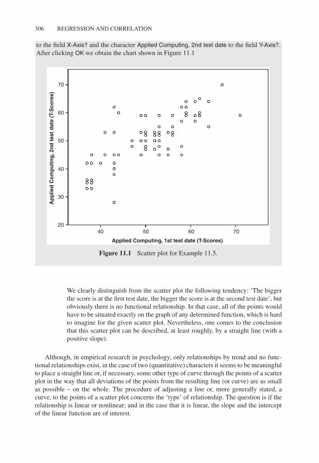
to the field X-Axis? and the character Applied Computing, 2nd test date to the field Y-Axis?.After clicking OK we obtain the chart shown in Figure 11.1
70
60
50
40
40 50 60
Applied Computing, 1st test date (T-Scores)
Ap
plie
d C
om
pu
tin
g, 2
nd
tes
t d
ate
(T-S
core
s)
70
30
20
Figure 11.1 Scatter plot for Example 11.5.
We clearly distinguish from the scatter plot the following tendency: ‘The biggerthe score is at the first test date, the bigger the score is at the second test date’, butobviously there is no functional relationship. In that case, all of the points wouldhave to be situated exactly on the graph of any determined function, which is hardto imagine for the given scatter plot. Nevertheless, one comes to the conclusionthat this scatter plot can be described, at least roughly, by a straight line (with apositive slope).
Although, in empirical research in psychology, only relationships by trend and no func-tional relationships exist, in the case of two (quantitative) characters it seems to be meaningfulto place a straight line or, if necessary, some other type of curve through the points of a scatterplot in the way that all deviations of the points from the resulting line (or curve) are as smallas possible – on the whole. The procedure of adjusting a line or, more generally stated, acurve, to the points of a scatter plot concerns the ‘type’ of relationship. The question is if therelationship is linear or nonlinear; and in the case that it is linear, the slope and the interceptof the linear function are of interest.
P1: OTA/XYZ P2: ABCJWST094-c11 JWST094-Rasch September 22, 2011 16:25 Printer Name: Yet to Come
INTRODUCTION 307
Bachelor Obviously, it is always feasible to fit a mathematical function (e.g. a straightline) in the best way possible to a scatter plot. However, the essential questionis to what extent the adjustment succeeds. It is always about how distant thesingle points of the scatter plot are from the curve that belongs to the func-tion. In the case of a relationship of 100%, all of the points would be situatedexactly on it.
The question of the type of relationship is the subject of the so-called regression analysis.Initially the appropriate model is selected; that is the determination of the type of function.In psychology this is almost always the linear function. The next step is to concretize thechosen function; that is, to find that one which adjusts to the scatter plot as well as possible.If this concretization were done by appearance in a subjective way, the result would be tooinexact. An exact determination can be made by means of a certain numeric procedure, theleast squares method (see Section 6.5). From a formal point of view, this means that theslope and intercept of the so-called regression line have to be determined in the best waypossible.
Bachelor After having exactly determined the type of relationship between two characters,as concerns future research units the outcome for one of the characters can bepredicted from the outcome of the other character. For that purpose, the graph ofthe mathematical function, which has finally been chosen, has to be positionedin a way that the overall differences (over all pairs of observations) between thetrue value and that value determined by the other character based on the givenrelationship, becomes a minimum. That is how the term ‘regression’ derives fromLatin (‘move backwards’), in the way that a certain point on the abscissa isprojected, via the respective mathematical function, onto the corresponding valueon the ordinate.
Doctor Generally, in regression analysis two different cases have to be distinguished:there are two different types of pairs of outcomes. In the case which is usualin psychology, both these values of each research unit were ascertained (mostlysimultaneously) by observation, and result as a matter of fact (so-called modelII). In contrast, in the other type (model I), the pair of outcomes consists of onevalue (e.g. the value x), which is chosen (purposely) in advance by the researcherbut only the other value (y) is observed as a matter of course. This type is rarelyfound in psychology. An example of this model is the observation of children’sgrowth between the age of 6 and 12 years. The investigator thus determines theage at which the body size of the children is measured. In this case, the x-valuesare not measured, but determined a priori.
The type of the model influences the calculation of slope and intercept ofthe regression line. More detailed information concerning model I in combina-tion with regression analysis can be found for example in Rasch, Verdooren, &Gowers (2007).
P1: OTA/XYZ P2: ABCJWST094-c11 JWST094-Rasch September 22, 2011 16:25 Printer Name: Yet to Come
308 REGRESSION AND CORRELATION
11.2 Regression model
If we model the characters x and y by two random variables x and y, then (x, y) is called abivariate random variable. Then the regression model is
yv = f (xv ) + ev (v = 1, 2, . . . , n) (11.1)
or
xv = g( yv ) + e′v (v = 1, 2, . . . , n) (11.2)
The function f is called a regression function from y onto x and the function g is called aregression function from x onto y. In function f , y is the regressand and x is the regressor, andvice versa in function g. The random variables ev or e′
v describe error terms. The model partic-ularly assumes that these errors are distributed with mean 0 and the same (mostly unknown)variance in each research unit v. It is also assumed that the error terms are independent fromeach other, as well as that the errors are independent from the variables x or y, respectively.
If functions f and g are linear functions, the following regression models result:
yv = β0 + β1xv + ev (v = 1, 2, . . . , n) (11.3)
or
xv = β ′0 + β ′
1 yv + e′v (v = 1, 2, . . . , n) (11.4)
respectively. If the random variables x and y are (two-dimensional) normally distributed, theregression function is always linear.
Usually the two functions y = β0 + β1x and x = β ′0 + β ′
1 y differ from each other. Theyare identical exclusively in the case that the strength of the relationship is maximal.
We thus have defined the regression model for the population. Now, we have to estimatethe adequate parameters β0 and β1 or β ′
0 and β ′1, respectively, with the help of a random
sample taken from the relevant population. With regard to the content, this is of interestmainly because, in practice, sometimes only one of the values (e.g. x-value) is known andwe want to ‘predict’ the corresponding one (y-value) in the best way possible. For both ofthe random variables x and y we will denote, in addition to the parameters of the regressionmodel, means and variances as follows: μx and μy, σ 2
x and σ 2y .
Starting from the need to place the regression line through the scatter plot in the waythat the overall differences between the true value and the value determinable from theother character’s value (based on the given relationship) are minimized, the estimates for theunknown parameters in the population, for instance for yv = β0 + β1xv + ev, can be given asfollows:
b0 = β0 = −b1 x (11.5)
b1 = β1 =1
n−1
n∑
v=1(xv − x) (yv − y)
s2x
(11.6)
P1: OTA/XYZ P2: ABCJWST094-c11 JWST094-Rasch September 22, 2011 16:25 Printer Name: Yet to Come
REGRESSION MODEL 309
Here s2x is the estimate of σ 2
x . The equation for the estimated regression line is now y =b1x + b0; thus for a concrete research unit v, yv = b1xv + b0.
Doctor Replacing the outcomes xv and yv in Formula (11.5) and (11.6) by the randomvariables xv and yv, by which these outcomes are modeled, we obtain the corre-sponding estimators; these are unbiased.
Master What was sloppily called overall ‘difference’ between the true value, yv, and thatvalue determined by the other character based on the given relationship, yv , is,from a formal point of view, a sum of squares. The sum of squares has basicallythe same function here as the absolute value of differences, but it possessesparticular statistical advantages compared to the absolute value. Thus β0 and β1
are estimated by β0 and β1 such that
n∑
v=1
(yv − yv )2 =n∑
v=1
[yv − (
β1xv + β0)]2
takes a minimum. The solution is found by partial differentiation and setting thefirst derivative to zero. The resulting values, b0 = β0 and b1 = β1, thus constitutethe estimates.
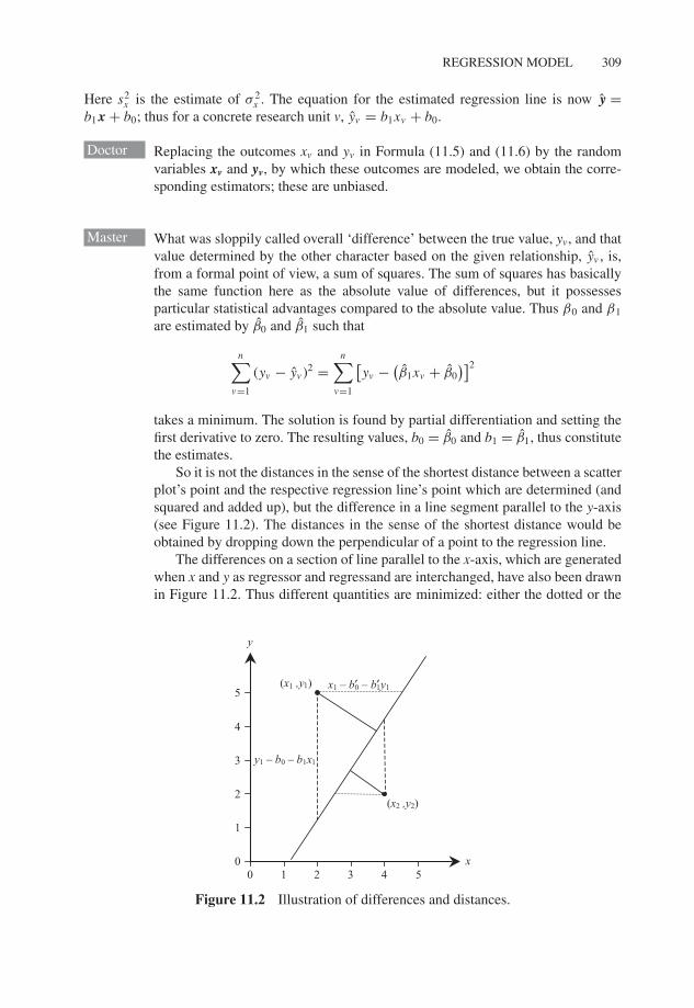
So it is not the distances in the sense of the shortest distance between a scatterplot’s point and the respective regression line’s point which are determined (andsquared and added up), but the difference in a line segment parallel to the y-axis(see Figure 11.2). The distances in the sense of the shortest distance would beobtained by dropping down the perpendicular of a point to the regression line.
The differences on a section of line parallel to the x-axis, which are generatedwhen x and y as regressor and regressand are interchanged, have also been drawnin Figure 11.2. Thus different quantities are minimized: either the dotted or the
x
y
0 1 2 3 40
1
2
3
4
x1 – b′0 – b′1y1
(x2 ,y2)
5
5(x1 ,y1)
y1 – b0 – b1x1
Figure 11.2 Illustration of differences and distances.
P1: OTA/XYZ P2: ABCJWST094-c11 JWST094-Rasch September 22, 2011 16:25 Printer Name: Yet to Come
310 REGRESSION AND CORRELATION
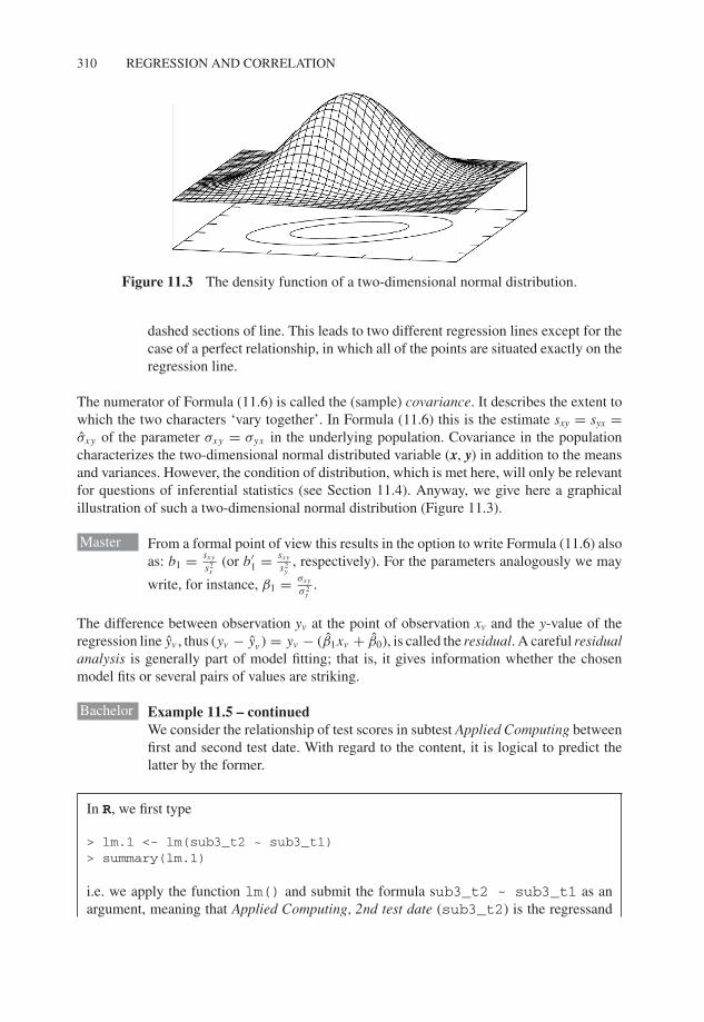
Figure 11.3 The density function of a two-dimensional normal distribution.
dashed sections of line. This leads to two different regression lines except for thecase of a perfect relationship, in which all of the points are situated exactly on theregression line.
The numerator of Formula (11.6) is called the (sample) covariance. It describes the extent towhich the two characters ‘vary together’. In Formula (11.6) this is the estimate sxy = syx =σxy of the parameter σxy = σyx in the underlying population. Covariance in the populationcharacterizes the two-dimensional normal distributed variable (x, y) in addition to the meansand variances. However, the condition of distribution, which is met here, will only be relevantfor questions of inferential statistics (see Section 11.4). Anyway, we give here a graphicalillustration of such a two-dimensional normal distribution (Figure 11.3).
Master From a formal point of view this results in the option to write Formula (11.6) alsoas: b1 = sxy
s2x
(or b′1 = sxy
s2y
, respectively). For the parameters analogously we may
write, for instance, β1 = σxy
σ 2y
.
The difference between observation yv at the point of observation xv and the y-value of theregression line yv , thus (yv − yv ) = yv − (β1xv + β0), is called the residual. A careful residualanalysis is generally part of model fitting; that is, it gives information whether the chosenmodel fits or several pairs of values are striking.
Bachelor Example 11.5 – continuedWe consider the relationship of test scores in subtest Applied Computing betweenfirst and second test date. With regard to the content, it is logical to predict thelatter by the former.
In R, we first type
> lm.1 <- lm(sub3_t2 ˜ sub3_t1)> summary(lm.1)
i.e. we apply the function lm() and submit the formula sub3_t2 ˜ sub3_t1 as anargument, meaning that Applied Computing, 2nd test date (sub3_t2) is the regressand
P1: OTA/XYZ P2: ABCJWST094-c11 JWST094-Rasch September 22, 2011 16:25 Printer Name: Yet to Come
REGRESSION MODEL 311
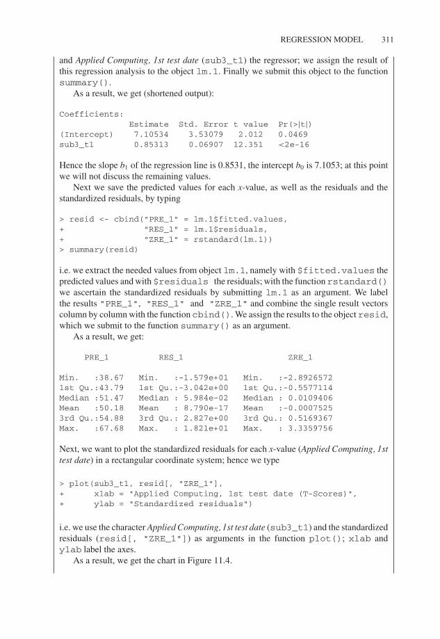
and Applied Computing, 1st test date (sub3_t1) the regressor; we assign the result ofthis regression analysis to the object lm.1. Finally we submit this object to the functionsummary().
As a result, we get (shortened output):
Coefficients:Estimate Std. Error t value Pr(>|t|)
(Intercept) 7.10534 3.53079 2.012 0.0469sub3_t1 0.85313 0.06907 12.351 <2e-16
Hence the slope b1 of the regression line is 0.8531, the intercept b0 is 7.1053; at this pointwe will not discuss the remaining values.
Next we save the predicted values for each x-value, as well as the residuals and thestandardized residuals, by typing
> resid <- cbind("PRE_1" = lm.1$fitted.values,+ "RES_1" = lm.1$residuals,+ "ZRE_1" = rstandard(lm.1))> summary(resid)
i.e. we extract the needed values from object lm.1, namely with $fitted.values thepredicted values and with $residuals the residuals; with the function rstandard()we ascertain the standardized residuals by submitting lm.1 as an argument. We labelthe results "PRE_1", "RES_1" and "ZRE_1" and combine the single result vectorscolumn by column with the function cbind(). We assign the results to the object resid,which we submit to the function summary() as an argument.
As a result, we get:
PRE_1 RES_1 ZRE_1
Min. :38.67 Min. :-1.579e+01 Min. :-2.89265721st Qu.:43.79 1st Qu.:-3.042e+00 1st Qu.:-0.5577114Median :51.47 Median : 5.984e-02 Median : 0.0109406Mean :50.18 Mean : 8.790e-17 Mean :-0.00075253rd Qu.:54.88 3rd Qu.: 2.827e+00 3rd Qu.: 0.5169367Max. :67.68 Max. : 1.821e+01 Max. : 3.3359756
Next, we want to plot the standardized residuals for each x-value (Applied Computing, 1sttest date) in a rectangular coordinate system; hence we type
> plot(sub3_t1, resid[, "ZRE_1"],+ xlab = "Applied Computing, 1st test date (T-Scores)",+ ylab = "Standardized residuals")
i.e. we use the character Applied Computing, 1st test date (sub3_t1) and the standardizedresiduals (resid[, "ZRE_1"]) as arguments in the function plot(); xlab andylab label the axes.
As a result, we get the chart in Figure 11.4.
P1: OTA/XYZ P2: ABCJWST094-c11 JWST094-Rasch September 22, 2011 16:25 Printer Name: Yet to Come
312 REGRESSION AND CORRELATION
40 45 50 55 60 65 70
Applied Computing, 1st test date (T-Scores)
Sta
nd
ard
ized
res
idu
als
–3–2
–10
12
3
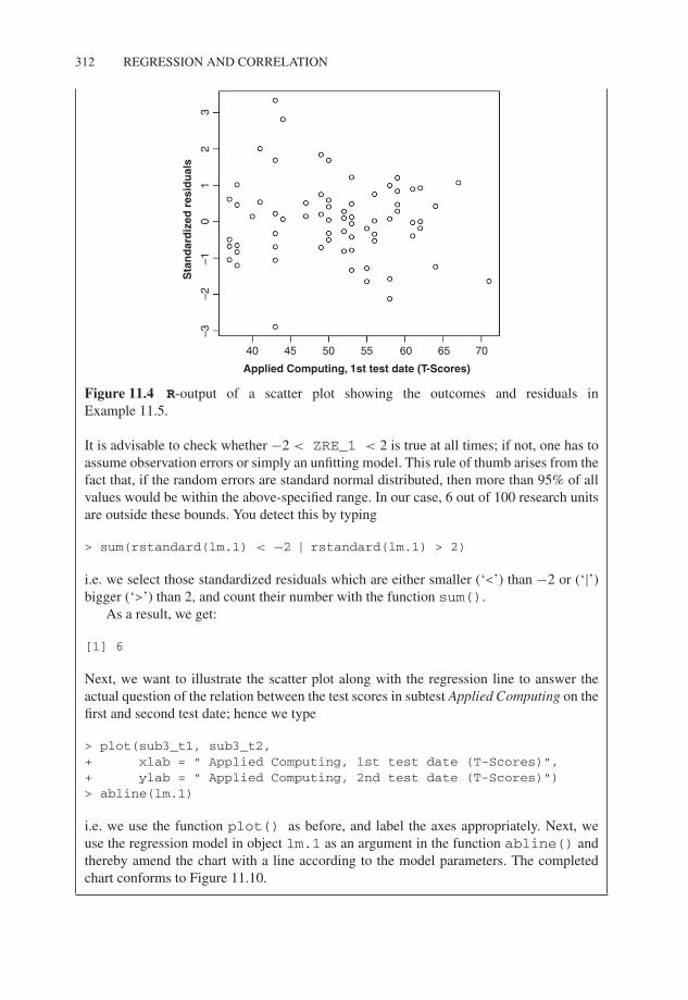
Figure 11.4 R-output of a scatter plot showing the outcomes and residuals inExample 11.5.
It is advisable to check whether −2 < ZRE_1 < 2 is true at all times; if not, one has toassume observation errors or simply an unfitting model. This rule of thumb arises from thefact that, if the random errors are standard normal distributed, then more than 95% of allvalues would be within the above-specified range. In our case, 6 out of 100 research unitsare outside these bounds. You detect this by typing
> sum(rstandard(lm.1) < −2 | rstandard(lm.1) > 2)
i.e. we select those standardized residuals which are either smaller (‘<’) than −2 or (‘|’)bigger (‘>’) than 2, and count their number with the function sum().
As a result, we get:
[1] 6
Next, we want to illustrate the scatter plot along with the regression line to answer theactual question of the relation between the test scores in subtest Applied Computing on thefirst and second test date; hence we type
> plot(sub3_t1, sub3_t2,+ xlab = " Applied Computing, 1st test date (T-Scores)",+ ylab = " Applied Computing, 2nd test date (T-Scores)")> abline(lm.1)
i.e. we use the function plot() as before, and label the axes appropriately. Next, weuse the regression model in object lm.1 as an argument in the function abline() andthereby amend the chart with a line according to the model parameters. The completedchart conforms to Figure 11.10.
P1: OTA/XYZ P2: ABCJWST094-c11 JWST094-Rasch September 22, 2011 16:25 Printer Name: Yet to Come
REGRESSION MODEL 313
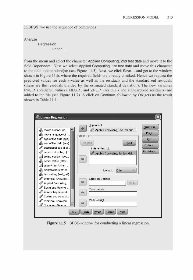
In SPSS, we use the sequence of commands
AnalyzeRegression
Linear. . .
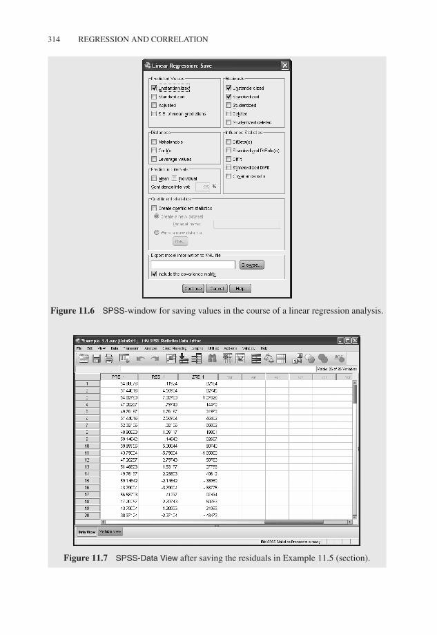
from the menu and select the character Applied Computing, 2nd test date and move it to thefield Dependent:. Next we select Applied Computing, 1st test date and move this characterto the field Independent(s): (see Figure 11.5). Next, we click Save. . . and get to the windowshown in Figure 11.6, where the required fields are already checked. Hence we request thepredicted values for each x-value as well as the residuals and the standardized residuals(these are the residuals divided by the estimated standard deviation). The new variablesPRE_1 (predicted values), RES_1, and ZRE_1 (residuals and standardized residuals) areadded to the file (see Figure 11.7). A click on Continue, followed by OK gets us the resultshown in Table 11.1.
Figure 11.5 SPSS-window for conducting a linear regression.
P1: OTA/XYZ P2: ABCJWST094-c11 JWST094-Rasch September 22, 2011 16:25 Printer Name: Yet to Come
314 REGRESSION AND CORRELATION
Figure 11.6 SPSS-window for saving values in the course of a linear regression analysis.
Figure 11.7 SPSS-Data View after saving the residuals in Example 11.5 (section).
P1: OTA/XYZ P2: ABCJWST094-c11 JWST094-Rasch September 22, 2011 16:25 Printer Name: Yet to Come
REGRESSION MODEL 315
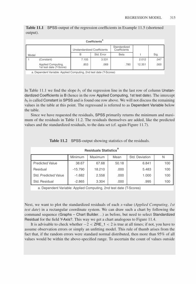
Table 11.1 SPSS-output of the regression coefficients in Example 11.5 (shortenedoutput).
Std. ErrorB Beta Sig.t
StandardizedCoefficientsUnstandardized Coefficients
(Constant)
Applied Computing,1st test date (T-Score)
1
.00012.351.780.069.853
.0472.0123.5317.105
Model
Coefficientsa
a. Dependent Variable: Applied Computing, 2nd test date (T-Scores)
In Table 11.1 we find the slope b1 of the regression line in the last row of column Unstan-dardized Coefficients in B (hence in the row Applied Computing, 1st test date). The interceptb0 is called Constant in SPSS and is found one row above. We will not discuss the remainingvalues in the table at this point. The regressand is referred to as Dependent Variable belowthe table.
Since we have requested the residuals, SPSS primarily returns the minimum and maxi-mum of the residuals in Table 11.2. The residuals themselves are added, like the predictedvalues and the standardized residuals, to the data set (cf. again Figure 11.7).
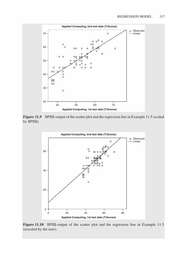
Table 11.2 SPSS-output showing statistics of the residuals.
NStd. DeviationMeanMaximumMinimum
Predicted Value
Residual
Std. Predicted Value
Std. Residual 100.995.0003.304-2.865
1001.000.0002.558-1.682
1005.483.00018.210-15.790
1006.84150.1867.6838.67
Residuals Statisticsa
a. Dependent Variable: Applied Computing, 2nd test date (T-Scores)
Next, we want to plot the standardized residuals of each x-value (Applied Computing, 1sttest date) in a rectangular coordinate system. We can draw such a chart by following thecommand sequence (Graphs – Chart Builder. . .) as before, but need to select StandardizedResidual for the field Y-Axis?. This way we get a chart analogous to Figure 11.4.
It is advisable to check whether −2 < ZRE_1 < 2 is true at all times; if not, you have toassume observation errors or simply an unfitting model. This rule of thumb arises from thefact that, if the random errors were standard normal distributed, then more than 95% of allvalues would be within the above-specified range. To ascertain the count of values outside

P1: OTA/XYZ P2: ABCJWST094-c11 JWST094-Rasch September 22, 2011 16:25 Printer Name: Yet to Come
316 REGRESSION AND CORRELATION
these bounds, we would need to create a frequency table as shown in Example 5.2, fromwhich we refrain here. That such cases even exist can be seen in Table 11.2, in the Row Std.Residual in the columns Minimum and Maximum.
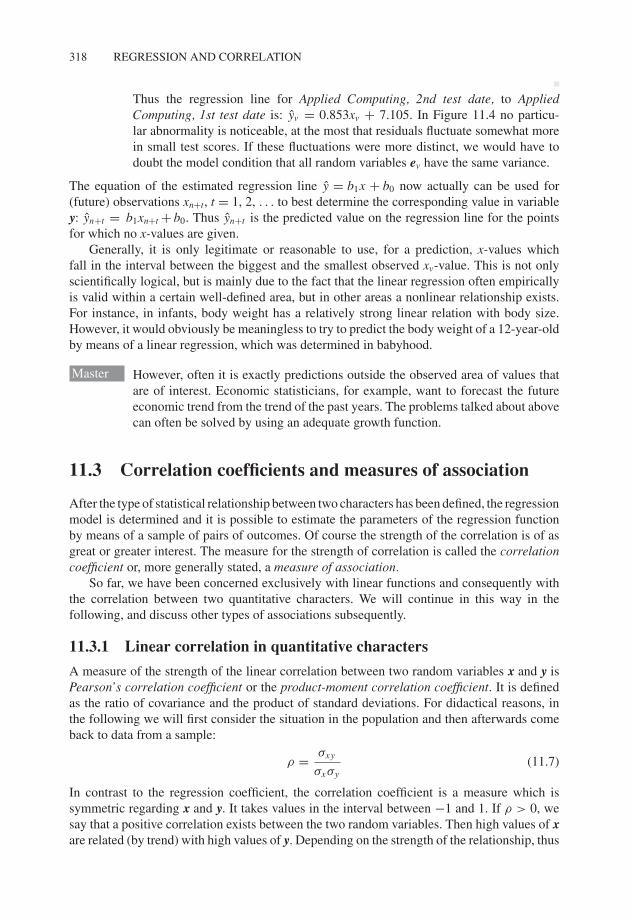
Next, we finally want to illustrate the scatter plot along with the regression line to answerthe actual question of the relation between the test scores in subtest Applied Computing onthe first and second test date; hence we select
AnalyzeRegression
Curve Estimation. . .
and get to the window shown in Figure 11.8. Here we keep the default selection of Linear,move the character Applied Computing, 2nd test date to the field Dependent(s): and thecharacter Applied Computing, 1st test date to the field Variable: in the panel Independent.With OK we get the desired chart (Figure 11.9). Double-clicking the chart starts the ChartEditor (see Figure 6.4), which we can use to, e.g., rescale the chart, so that the zero value forboth variables is shown. We do that by selecting Edit from the menu bar and clicking SelectX Axis. Subsequently a new window pops up (not illustrated), where we change the value inrow Minimum in field Custom to 0, Apply this setting and close the window. We repeat thisprocedure for the sequence of commands Edit – Select Y Axis. Now we can close the ChartEditor and, as a result, we get Figure 11.10.
Figure 11.8 SPSS-window for creating a scatter plot as well as a regression line.
P1: OTA/XYZ P2: ABCJWST094-c11 JWST094-Rasch September 22, 2011 16:25 Printer Name: Yet to Come
REGRESSION MODEL 317
70
60
50
40
30
2040 50 60
Applied Computing, 1st test date (T-Scores)
Applied Computing, 2nd test date (T-Scores)
ObservedLinear
70
Figure 11.9 SPSS-output of the scatter plot and the regression line in Example 11.5 (scaledby SPSS).
60
40
20
00 20 40 60
Applied Computing, 1st test date (T-Scores)
Applied Computing, 2nd test date (T-Scores)
ObservedLinear
80
Figure 11.10 SPSS-output of the scatter plot and the regression line in Example 11.5(rescaled by the user).
P1: OTA/XYZ P2: ABCJWST094-c11 JWST094-Rasch September 22, 2011 16:25 Printer Name: Yet to Come
318 REGRESSION AND CORRELATION
Thus the regression line for Applied Computing, 2nd test date, to AppliedComputing, 1st test date is: yv = 0.853xv + 7.105. In Figure 11.4 no particu-lar abnormality is noticeable, at the most that residuals fluctuate somewhat morein small test scores. If these fluctuations were more distinct, we would have todoubt the model condition that all random variables ev have the same variance.
The equation of the estimated regression line y = b1x + b0 now actually can be used for(future) observations xn+t, t = 1, 2, . . . to best determine the corresponding value in variabley: yn+t = b1xn+t + b0. Thus yn+t is the predicted value on the regression line for the pointsfor which no x-values are given.
Generally, it is only legitimate or reasonable to use, for a prediction, x-values whichfall in the interval between the biggest and the smallest observed xv-value. This is not onlyscientifically logical, but is mainly due to the fact that the linear regression often empiricallyis valid within a certain well-defined area, but in other areas a nonlinear relationship exists.For instance, in infants, body weight has a relatively strong linear relation with body size.However, it would obviously be meaningless to try to predict the body weight of a 12-year-oldby means of a linear regression, which was determined in babyhood.
Master However, often it is exactly predictions outside the observed area of values thatare of interest. Economic statisticians, for example, want to forecast the futureeconomic trend from the trend of the past years. The problems talked about abovecan often be solved by using an adequate growth function.
11.3 Correlation coefficients and measures of association
After the type of statistical relationship between two characters has been defined, the regressionmodel is determined and it is possible to estimate the parameters of the regression functionby means of a sample of pairs of outcomes. Of course the strength of the correlation is of asgreat or greater interest. The measure for the strength of correlation is called the correlationcoefficient or, more generally stated, a measure of association.
So far, we have been concerned exclusively with linear functions and consequently withthe correlation between two quantitative characters. We will continue in this way in thefollowing, and discuss other types of associations subsequently.
11.3.1 Linear correlation in quantitative characters
A measure of the strength of the linear correlation between two random variables x and y isPearson’s correlation coefficient or the product-moment correlation coefficient. It is definedas the ratio of covariance and the product of standard deviations. For didactical reasons, inthe following we will first consider the situation in the population and then afterwards comeback to data from a sample:
ρ = σxy
σxσy(11.7)
In contrast to the regression coefficient, the correlation coefficient is a measure which issymmetric regarding x and y. It takes values in the interval between −1 and 1. If ρ > 0, wesay that a positive correlation exists between the two random variables. Then high values of xare related (by trend) with high values of y. Depending on the strength of the relationship, thus
P1: OTA/XYZ P2: ABCJWST094-c11 JWST094-Rasch September 22, 2011 16:25 Printer Name: Yet to Come
CORRELATION COEFFICIENTS AND MEASURES OF ASSOCIATION 319
the absolute value of ρ, the relation is more or less consistent. If ρ < 0, we say that a negativecorrelation exists between the two random variables. Then high values of x are related (bytrend) with small values of y. If the two random variables are independent from each other,thus ‘uncorrelated’, the covariance is σ xy = 0, and therefore also the correlation coefficient ρ
= 0 and both of the regression coefficients β1, β ′1. Nevertheless, if, for two random variables,
ρ = 0, then they are not necessarily independent from one another. But, a linear relation doesnot exist in any case.
Master Pearson’s correlation coefficient can be deduced intuitively as follows.First we reflect on the question of for which cases we would consider a
correlation between two characters as relevant, for instance relevant to an extentthat it seems to be meaningful to predict an unknown value yi from xi by means ofthe regression line. Now, the correlation would surely be considered as relevantand such a prediction as meaningful, if the character x, modeled by x, could‘explain’ ‘why’ the observations of the other character y, modeled by y, take,exactly, certain realizations yv, v = 1, 2, . . . , n.
We assume here that we are interested in the correlation between intelligence(intelligence test with test score x) and school achievement (school achievementtest with test score y), which is indeed the subject of many debates. Schoolachievement thus is to be modeled by a random variable, which will certainly notlead to the same outcomes in all children, but to outcomes with a certain variabil-ity, measured by variance. If intelligence, as the other modeled random variable,is capable of explaining this variability in the way that high school achievementoften is related to high intelligence and low school achievement to low intelli-gence, then the following question arises: to what extent exactly is the intelligence‘responsible’ for the variability in school achievement of these children? It is im-portant to note that causality between the two characters is not presumed thereby.That is to say that it is equally possible, with regard to the content, that, in-versely, differences in school achievement cause the corresponding differences inthe intelligence test. It is also possible that the differences between the childrenconcerning school achievement as well as intelligence test achievement are dueto differences between the children in the trait ‘achievement motivation’.
Thus the question is about the extent of variance σ 2y in school achievement,
which is determined (we also say: described) solely by the variance in intelligence.Provided that the regression from y onto x is given, we can determine the valueyv = y(xv ) = b0 + b1xv for each research unit v. Calculating the variance s2
y of allof these values yv , we obtain the estimation for σ 2
y of y of that fraction of varianceof y, σ 2
y , which can be described (or predicted, respectively) or determined for thegiven population from x. It is of interest now to relate this variance σ 2
y to the totalvariance of y (within the population), thus to calculate the relative proportion of
variance explained by x:σ 2
y
σ 2y.
Since
σ 2y = E [ y − E ( y)]2 = E [b0 + b1x − E (b0 + b1x)]2 = β2
1 · E [x − E(x)]2
=(
σxy
σ 2x
)2
· σ 2x = σ 2
xy
σ 2x
P1: OTA/XYZ P2: ABCJWST094-c11 JWST094-Rasch September 22, 2011 16:25 Printer Name: Yet to Come
320 REGRESSION AND CORRELATION
32
10y
–1–2
–3
–3 –2 –1 0 1 2 3x
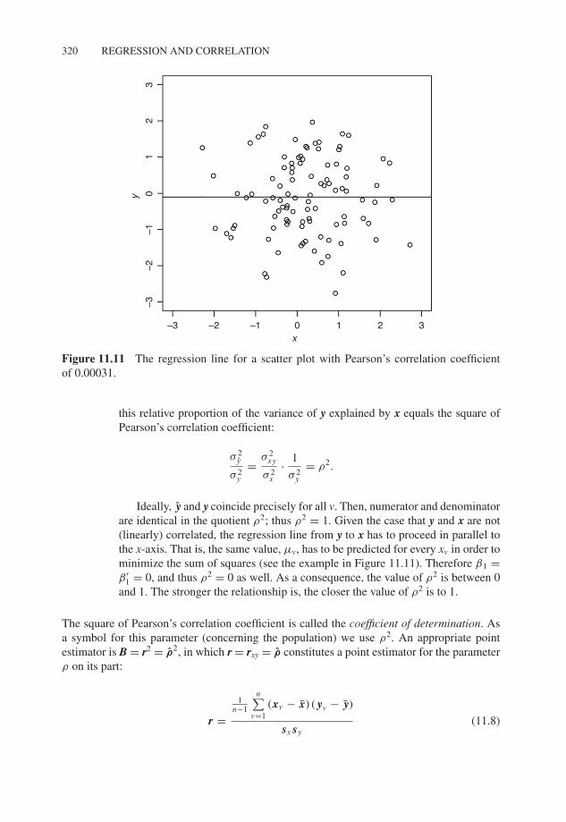
Figure 11.11 The regression line for a scatter plot with Pearson’s correlation coefficientof 0.00031.
this relative proportion of the variance of y explained by x equals the square ofPearson’s correlation coefficient:
σ 2y
σ 2y
= σ 2xy
σ 2x
· 1
σ 2y
= ρ2.
Ideally, y and y coincide precisely for all v. Then, numerator and denominatorare identical in the quotient ρ2; thus ρ2 = 1. Given the case that y and x are not(linearly) correlated, the regression line from y to x has to proceed in parallel tothe x-axis. That is, the same value, μv, has to be predicted for every xv in order tominimize the sum of squares (see the example in Figure 11.11). Therefore β1 =β ′
1 = 0, and thus ρ2 = 0 as well. As a consequence, the value of ρ2 is between 0and 1. The stronger the relationship is, the closer the value of ρ2 is to 1.
The square of Pearson’s correlation coefficient is called the coefficient of determination. Asa symbol for this parameter (concerning the population) we use ρ2. An appropriate pointestimator is B = r2 = ρ2, in which r = rxy = ρ constitutes a point estimator for the parameterρ on its part:
r =1
n−1
n∑
v=1(xv − x) ( yv − y)
sx sy(11.8)
P1: OTA/XYZ P2: ABCJWST094-c11 JWST094-Rasch September 22, 2011 16:25 Printer Name: Yet to Come
CORRELATION COEFFICIENTS AND MEASURES OF ASSOCIATION 321
Master The estimator r for ρ in Formula (11.8) is not unbiased. An unbiased estimatoralso exists, but as the bias is not too big, we recommend using Formula (11.8),nevertheless.
Bachelor A coefficient of determination of, for instance, B = 0.81 (thus r = 0.9) means that81% of the variance in y can be explained by the variance in x (and vice versa).Then, 19% of the variance (the variability) of y depends on other, unknown(influencing) factors. A coefficient of determination of B = 0.49 (thus r = 0.7)indicates that almost half of the variance of the variables is explained mutually.This can be referred to as a medium-sized correlation. If the correlation coefficientequals 0.3 and therefore the coefficient of determination B = 0.09, not even 10%of the variance is being explained mutually. In most cases, this relationship is notrelevant in a practical sense.
For Lecturers:
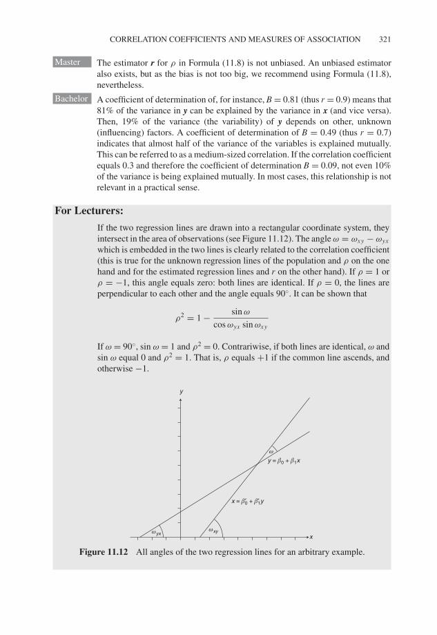
If the two regression lines are drawn into a rectangular coordinate system, theyintersect in the area of observations (see Figure 11.12). The angle ω = ωxy − ωyx
which is embedded in the two lines is clearly related to the correlation coefficient(this is true for the unknown regression lines of the population and ρ on the onehand and for the estimated regression lines and r on the other hand). If ρ = 1 orρ = −1, this angle equals zero: both lines are identical. If ρ = 0, the lines areperpendicular to each other and the angle equals 90◦. It can be shown that
ρ2 = 1 − sin ω
cos ωyx sin ωxy
If ω = 90◦, sin ω = 1 and ρ2 = 0. Contrariwise, if both lines are identical, ω andsin ω equal 0 and ρ2 = 1. That is, ρ equals +1 if the common line ascends, andotherwise −1.
y
ω
y = β0 + β1x
x = β′0 + β′1y
ωyxωxy
x
Figure 11.12 All angles of the two regression lines for an arbitrary example.
P1: OTA/XYZ P2: ABCJWST094-c11 JWST094-Rasch September 22, 2011 16:25 Printer Name: Yet to Come
322 REGRESSION AND CORRELATION
Generally, we caution against calculating the correlation coefficient uncritically; that iswithout making sure in advance by means of a graph that the assumed relationship is in factlinear.
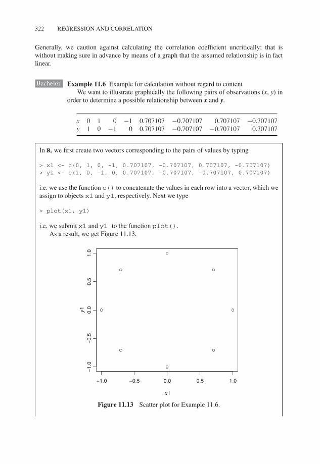
Bachelor Example 11.6 Example for calculation without regard to contentWe want to illustrate graphically the following pairs of observations (x, y) in
order to determine a possible relationship between x and y.
x 0 1 0 −1 0.707107 −0.707107 0.707107 −0.707107y 1 0 −1 0 0.707107 −0.707107 −0.707107 0.707107
In R, we first create two vectors corresponding to the pairs of values by typing
> x1 <- c(0, 1, 0, -1, 0.707107, -0.707107, 0.707107, -0.707107)> y1 <- c(1, 0, -1, 0, 0.707107, -0.707107, -0.707107, 0.707107)
i.e. we use the function c() to concatenate the values in each row into a vector, which weassign to objects x1 and y1, respectively. Next we type
> plot(x1, y1)
i.e. we submit x1 and y1 to the function plot().As a result, we get Figure 11.13.
−1.0 −0.5 0.0 0.5 1.0
−1.
0−
0.5
0.0
0.5
1.0
x1
y1
Figure 11.13 Scatter plot for Example 11.6.
P1: OTA/XYZ P2: ABCJWST094-c11 JWST094-Rasch September 22, 2011 16:25 Printer Name: Yet to Come
CORRELATION COEFFICIENTS AND MEASURES OF ASSOCIATION 323
Next, we ascertain the extent of the linear relationship by typing
> cor(x1, y1, method = "pearson")
i.e. we use both variables, x1 and y1, as arguments in the function cor(); with method= "pearson" we select Pearson’s correlation coefficient.
As a result, we get:
[1] 0
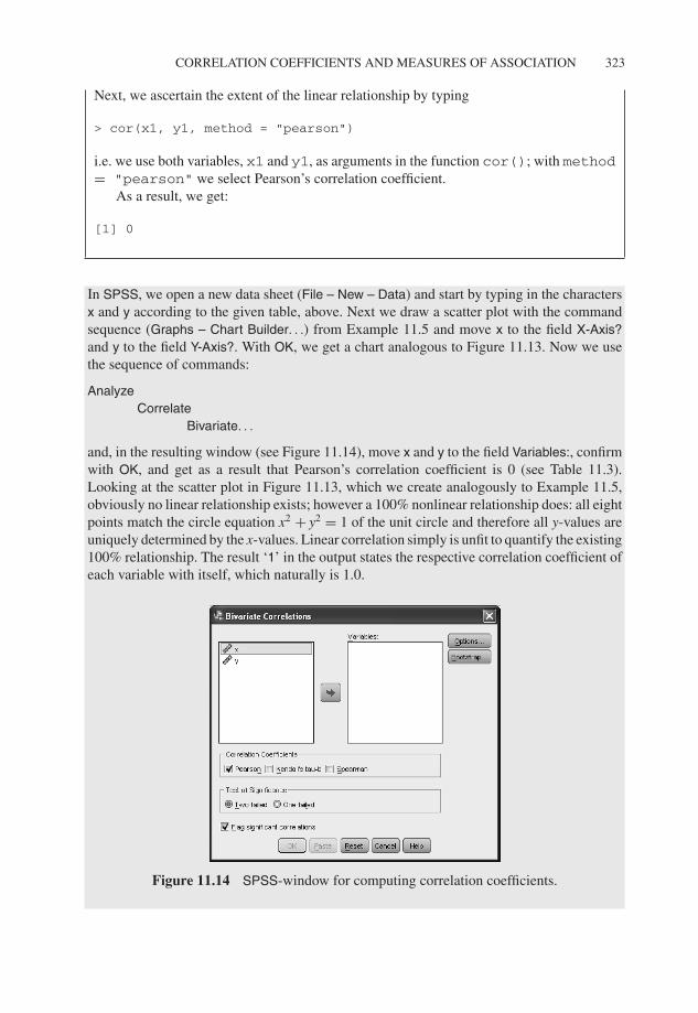
In SPSS, we open a new data sheet (File – New – Data) and start by typing in the charactersx and y according to the given table, above. Next we draw a scatter plot with the commandsequence (Graphs – Chart Builder. . .) from Example 11.5 and move x to the field X-Axis?and y to the field Y-Axis?. With OK, we get a chart analogous to Figure 11.13. Now we usethe sequence of commands:
AnalyzeCorrelate
Bivariate. . .
and, in the resulting window (see Figure 11.14), move x and y to the field Variables:, confirmwith OK, and get as a result that Pearson’s correlation coefficient is 0 (see Table 11.3).Looking at the scatter plot in Figure 11.13, which we create analogously to Example 11.5,obviously no linear relationship exists; however a 100% nonlinear relationship does: all eightpoints match the circle equation x2 + y2 = 1 of the unit circle and therefore all y-values areuniquely determined by the x-values. Linear correlation simply is unfit to quantify the existing100% relationship. The result ‘1’ in the output states the respective correlation coefficient ofeach variable with itself, which naturally is 1.0.
Figure 11.14 SPSS-window for computing correlation coefficients.
P1: OTA/XYZ P2: ABCJWST094-c11 JWST094-Rasch September 22, 2011 16:25 Printer Name: Yet to Come
324 REGRESSION AND CORRELATION
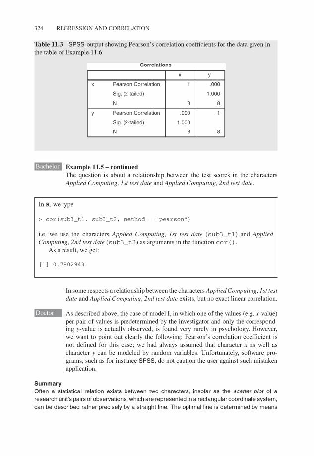
Table 11.3 SPSS-output showing Pearson’s correlation coefficients for the data given inthe table of Example 11.6.
yx
Pearson Correlation
Sig. (2-tailed)
N
Pearson Correlation
Sig. (2-tailed)
N
x
y
88
1.000
1.000
88
1.000
.0001
Correlations
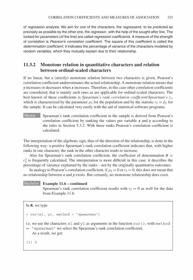
Bachelor Example 11.5 – continuedThe question is about a relationship between the test scores in the charactersApplied Computing, 1st test date and Applied Computing, 2nd test date.
In R, we type
> cor(sub3_t1, sub3_t2, method = "pearson")
i.e. we use the characters Applied Computing, 1st test date (sub3_t1) and AppliedComputing, 2nd test date (sub3_t2) as arguments in the function cor().
As a result, we get:
[1] 0.7802943
In some respects a relationship between the characters Applied Computing, 1st testdate and Applied Computing, 2nd test date exists, but no exact linear correlation.
Doctor As described above, the case of model I, in which one of the values (e.g. x-value)per pair of values is predetermined by the investigator and only the correspond-ing y-value is actually observed, is found very rarely in psychology. However,we want to point out clearly the following: Pearson’s correlation coefficient isnot defined for this case; we had always assumed that character x as well ascharacter y can be modeled by random variables. Unfortunately, software pro-grams, such as for instance SPSS, do not caution the user against such mistakenapplication.
SummaryOften a statistical relation exists between two characters, insofar as the scatter plot of aresearch unit’s pairs of observations, which are represented in a rectangular coordinate system,can be described rather precisely by a straight line. The optimal line is determined by means
P1: OTA/XYZ P2: ABCJWST094-c11 JWST094-Rasch September 22, 2011 16:25 Printer Name: Yet to Come
CORRELATION COEFFICIENTS AND MEASURES OF ASSOCIATION 325
of regression analysis. We aim for one of the characters, the regressand, to be predicted asprecisely as possible by the other one, the regressor , with the help of the sought-after line. Thelooked-for parameters (of the line) are called regression coefficients. A measure of the strengthof correlation is Pearson’s correlation coefficient. The square of this coefficient is called thedetermination coefficient; it indicates the percentage of variance of the characters modeled byrandom variables, which they mutually explain due to their relationship.
11.3.2 Monotone relation in quantitative characters and relationbetween ordinal-scaled characters
If no linear, but a (strictly) monotone relation between two characters is given, Pearson’scorrelation coefficient underestimates the actual relationship. A monotone relation means thaty increases or decreases when x increases. Therefore, in this case other correlation coefficientsare considered; that is mainly such ones as are applicable for ordinal-scaled characters. Thebest known of these coefficients is Spearman’s rank correlation coefficient/Spearman’s rs,which is characterized by the parameter ρS for the population and by the statistic rS = ρS forthe sample. It can be calculated very easily with the aid of statistical software programs.
Master Spearman’s rank correlation coefficient in the sample is derived from Pearson’scorrelation coefficient by ranking the values per variable x and y according tothe rules in Section 5.3.2. With these ranks Pearson’s correlation coefficient iscalculated.
The interpretation of the algebraic sign, thus of the direction of the relationship, is done in thefollowing way: a positive Spearman’s rank correlation coefficient indicates that, with higherranks in one character, the rank in the other character tends to increase.
Also for Spearman’s rank correlation coefficient, the coefficient of determination B =r2
S is frequently calculated. The interpretation is more difficult in this case: it describes thepercentage of variance explained by the ranks – not by the originally quantitative outcomes.
In analogy to Pearson’s correlation coefficient, if ρS = 0 or rS = 0, this does not mean thatno relationship between x and y exists. But certainly, no monotone relationship does exist.
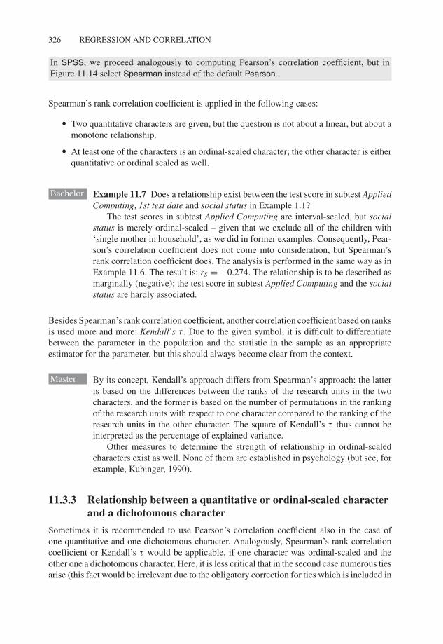
Bachelor Example 11.6 – continuedSpearman’s rank correlation coefficient results with rS = 0 as well for the datafrom Example 11.6.
In R, we type
> cor(x1, y1, method = "spearman")
i.e. we use the characters x1 and y1 as arguments in the function cor(); with method= "spearman" we select the Spearman’s rank correlation coefficient.
As a result, we get:
[1] 0
P1: OTA/XYZ P2: ABCJWST094-c11 JWST094-Rasch September 22, 2011 16:25 Printer Name: Yet to Come
326 REGRESSION AND CORRELATION
In SPSS, we proceed analogously to computing Pearson’s correlation coefficient, but inFigure 11.14 select Spearman instead of the default Pearson.
Spearman’s rank correlation coefficient is applied in the following cases:
� Two quantitative characters are given, but the question is not about a linear, but about amonotone relationship.
� At least one of the characters is an ordinal-scaled character; the other character is eitherquantitative or ordinal scaled as well.
Bachelor Example 11.7 Does a relationship exist between the test score in subtest AppliedComputing, 1st test date and social status in Example 1.1?
The test scores in subtest Applied Computing are interval-scaled, but socialstatus is merely ordinal-scaled – given that we exclude all of the children with‘single mother in household’, as we did in former examples. Consequently, Pear-son’s correlation coefficient does not come into consideration, but Spearman’srank correlation coefficient does. The analysis is performed in the same way as inExample 11.6. The result is: rS = −0.274. The relationship is to be described asmarginally (negative); the test score in subtest Applied Computing and the socialstatus are hardly associated.
Besides Spearman’s rank correlation coefficient, another correlation coefficient based on ranksis used more and more: Kendall’s τ . Due to the given symbol, it is difficult to differentiatebetween the parameter in the population and the statistic in the sample as an appropriateestimator for the parameter, but this should always become clear from the context.
Master By its concept, Kendall’s approach differs from Spearman’s approach: the latteris based on the differences between the ranks of the research units in the twocharacters, and the former is based on the number of permutations in the rankingof the research units with respect to one character compared to the ranking of theresearch units in the other character. The square of Kendall’s τ thus cannot beinterpreted as the percentage of explained variance.
Other measures to determine the strength of relationship in ordinal-scaledcharacters exist as well. None of them are established in psychology (but see, forexample, Kubinger, 1990).
11.3.3 Relationship between a quantitative or ordinal-scaled characterand a dichotomous character
Sometimes it is recommended to use Pearson’s correlation coefficient also in the case ofone quantitative and one dichotomous character. Analogously, Spearman’s rank correlationcoefficient or Kendall’s τ would be applicable, if one character was ordinal-scaled and theother one a dichotomous character. Here, it is less critical that in the second case numerous tiesarise (this fact would be irrelevant due to the obligatory correction for ties which is included in
P1: OTA/XYZ P2: ABCJWST094-c11 JWST094-Rasch September 22, 2011 16:25 Printer Name: Yet to Come
CORRELATION COEFFICIENTS AND MEASURES OF ASSOCIATION 327
the formula), than the fact that, in both cases, despite an ‘ideal’ relationship, in many instancesthe correlation coefficients cannot achieve the value of 1.
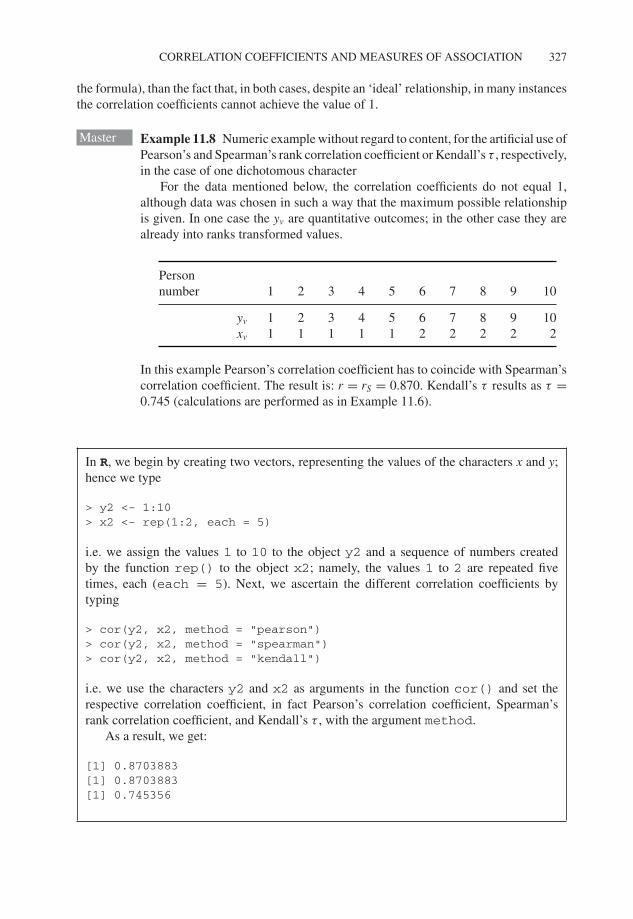
Master Example 11.8 Numeric example without regard to content, for the artificial use ofPearson’s and Spearman’s rank correlation coefficient or Kendall’s τ , respectively,in the case of one dichotomous character
For the data mentioned below, the correlation coefficients do not equal 1,although data was chosen in such a way that the maximum possible relationshipis given. In one case the yv are quantitative outcomes; in the other case they arealready into ranks transformed values.
Personnumber 1 2 3 4 5 6 7 8 9 10
yv 1 2 3 4 5 6 7 8 9 10xv 1 1 1 1 1 2 2 2 2 2
In this example Pearson’s correlation coefficient has to coincide with Spearman’scorrelation coefficient. The result is: r = rS = 0.870. Kendall’s τ results as τ =0.745 (calculations are performed as in Example 11.6).
In R, we begin by creating two vectors, representing the values of the characters x and y;hence we type
> y2 <- 1:10> x2 <- rep(1:2, each = 5)
i.e. we assign the values 1 to 10 to the object y2 and a sequence of numbers createdby the function rep() to the object x2; namely, the values 1 to 2 are repeated fivetimes, each (each = 5). Next, we ascertain the different correlation coefficients bytyping
> cor(y2, x2, method = "pearson")> cor(y2, x2, method = "spearman")> cor(y2, x2, method = "kendall")
i.e. we use the characters y2 and x2 as arguments in the function cor() and set therespective correlation coefficient, in fact Pearson’s correlation coefficient, Spearman’srank correlation coefficient, and Kendall’s τ , with the argument method.
As a result, we get:
[1] 0.8703883[1] 0.8703883[1] 0.745356
P1: OTA/XYZ P2: ABCJWST094-c11 JWST094-Rasch September 22, 2011 16:25 Printer Name: Yet to Come
328 REGRESSION AND CORRELATION
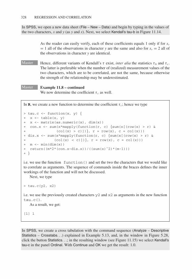
In SPSS, we open a new data sheet (File – New – Data) and begin by typing in the values ofthe two characters, x and y (as y and x). Next, we select Kendall’s tau-b in Figure 11.14.
As the reader can easily verify, each of these coefficients equals 1 only if for xv
= 1 all of the observations in character y are the same and also for xv = 2 all ofthe observations in character y are identical.
Master Hence, different variants of Kendall’s τ exist, inter alia the statistics τ b and τ c.The latter is preferable when the number of (realized) measurement values of thetwo characters, which are to be correlated, are not the same, because otherwisethe strength of the relationship may be underestimated.
Master Example 11.8 – continuedWe now determine the coefficient τ c as well.
In R, we create a new function to determine the coefficient τ c; hence we type
> tau.c <- function(x, y) {+ x <- table(x, y)+ x <- matrix(as.numeric(x), dim(x))+ con.x <- sum(x*mapply(function(r, c) {sum(x[(row(x) > r) &+ (col(x) > c)])}, r = row(x), c = col(x)))+ dis.x <- sum(x*mapply(function(r, c) {sum(x[(row(x) > r) &+ (col(x) < c)])}, r = row(x), c = col(x)))+ m <- min(dim(x))+ return((m*2*(con.x-dis.x))/((sum(x)ˆ2)*(m-1)))+ }
i.e. we use the function function() and set the two the characters that we would liketo correlate as arguments. The sequence of commands inside the braces defines the innerworkings of the function and will not be discussed.
Next, we type
> tau.c(y2, x2)
i.e. we use the previously created characters y2 and x2 as arguments in the new functiontau.c().
As a result, we get:
[1] 1
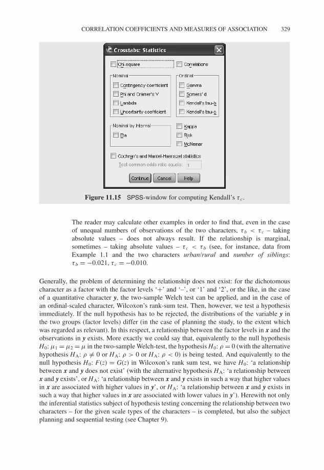
In SPSS, we create a cross tabulation with the command sequence (Analyze – DescriptiveStatistics – Crosstabs. . .) explained in Example 5.13, and, in the window in Figure 5.28,click the button Statistics. . .; in the resulting window (see Figure 11.15) we select Kendall’stau-c in the panel Ordinal. With Continue and OK we get the result: 1.0.
P1: OTA/XYZ P2: ABCJWST094-c11 JWST094-Rasch September 22, 2011 16:25 Printer Name: Yet to Come
CORRELATION COEFFICIENTS AND MEASURES OF ASSOCIATION 329
Figure 11.15 SPSS-window for computing Kendall’s τ c.
The reader may calculate other examples in order to find that, even in the caseof unequal numbers of observations of the two characters, τ b < τ c – takingabsolute values – does not always result. If the relationship is marginal,sometimes – taking absolute values – τ c < τ b (see, for instance, data fromExample 1.1 and the two characters urban/rural and number of siblings:τ b = −0.021, τ c = −0.010.
Generally, the problem of determining the relationship does not exist: for the dichotomouscharacter as a factor with the factor levels ‘+’ and ‘–’, or ‘1’ and ‘2’, or the like, in the caseof a quantitative character y, the two-sample Welch test can be applied, and in the case ofan ordinal-scaled character, Wilcoxon’s rank-sum test. Then, however, we test a hypothesisimmediately. If the null hypothesis has to be rejected, the distributions of the variable y inthe two groups (factor levels) differ (in the case of planning the study, to the extent whichwas regarded as relevant). In this respect, a relationship between the factor levels in x and theobservations in y exists. More exactly we could say that, equivalently to the null hypothesisH0: μ1 = μ2 = μ in the two-sample Welch-test, the hypothesis H0: ρ = 0 (with the alternativehypothesis HA: ρ �= 0 or HA: ρ > 0 or HA: ρ < 0) is being tested. And equivalently to thenull hypothesis H0: F(z) = G(z) in Wilcoxon’s rank sum test, we have H0: ‘a relationshipbetween x and y does not exist’ (with the alternative hypothesis HA: ‘a relationship betweenx and y exists’, or HA: ‘a relationship between x and y exists in such a way that higher valuesin x are associated with higher values in y’, or HA: ‘a relationship between x and y exists insuch a way that higher values in x are associated with lower values in y’). Herewith not onlythe inferential statistics subject of hypothesis testing concerning the relationship between twocharacters – for the given scale types of the characters – is completed, but also the subjectplanning and sequential testing (see Chapter 9).
P1: OTA/XYZ P2: ABCJWST094-c11 JWST094-Rasch September 22, 2011 16:25 Printer Name: Yet to Come
330 REGRESSION AND CORRELATION
Master Example 11.9 Item discriminatory powerWithin psychometrics, item discriminatory power describes the extent to
which a certain item of a psychological test is capable of discriminating in thesame way as the test as a whole (with the exception of the item in question)between persons with different intensities regarding the measured ability.
We assume that, for instance, we have m = 8 dichotomous charactersyl, l = 1, 2, . . . , m, items of a psychological test, which were observed in ntestees. Each item can be either ‘solved’ (= 1) or ‘not solved’ (= 0). Then, forexample, a new variable y∗
l = ∑8j=1, j �=l yl can be defined, that is the sum of all
solved items except the item which is considered at the moment, l. Subsequently,Pearson’s correlation coefficient between yl and y∗
l is calculated. Sometimes thisspecial case of a correlation between a quantitative and a dichotomous variable iscalled point-biserial correlation.
With regard to the considerations made above, the interpretation of itemdiscriminatory power based on the theoretical maximum value of 1 is not useful.It would be preferable to apply the two-sample Welch test and, if the study has notbeen planned (with targeted precision requirements), to interpret the estimatedeffect size.
11.3.4 Relationship between a quantitative character and amulti-categorical character
A method for quantifying the relationship between an ordinal-scaled and a multi-categorical(non-dichotomous) character does not exist in statistics. In this case, we have to downgradethe ordinal-scaled variable to the next-lower scale type; thus to exploit only the informationof a nominal scale (equal or unequal). This results in using that association measure which isavailable for two multi-categorical characters (see below in Section 11.3.5).
However, if the question is about a quantitative and a multi-categorical character, Fisher’scorrelation ratio/eta-squared is an appropriate association measure – again, because of thegiven symbol, it is difficult to differentiate between the parameter in the population and thestatistic in the sample as an appropriate estimator for the parameter. This coefficient can beeasily calculated with the help of statistical software as well, and it also often cannot reachthe value of 1 even in the case of an ‘ideal’ correlation.
MasterDoctor
With reference to Table 10.3, Fisher’s correlation ratio is defined by
η2 = SSA
SSt(11.9)
thus by the relation of the sum of squares of the level means yi concerning theoverall mean y and the sum of squares of the observations yiv concerning theoverall mean y; thereby, levels mean the different categories of the nominal-scaled character (see Section 10.4.1.1). The possible values of η2 are 0 ≤ η2 ≤ 1.η2 = 0 if yi = y for all i; then SSA or the variance of the level means, respectively,
P1: OTA/XYZ P2: ABCJWST094-c11 JWST094-Rasch September 22, 2011 16:25 Printer Name: Yet to Come
CORRELATION COEFFICIENTS AND MEASURES OF ASSOCIATION 331
equals zero. η2 = 1 results only if, for all v, yiv = yi happens to occur; thus if thecharacter y does not possess any variance per factor level i (compare the analogyto Section 11.3.3).
Master Example 11.8 – continuedThough the structure of data in this example is just a special case of all pos-sible applications of Fisher’s correlation ratio, it is nevertheless appropriate todemonstrate that this coefficient cannot reach a value of 1, despite an ‘ideal’relationship.
In R, we need to compute Fisher’s correlation ratio step by step; we start with typing
> summary(aov(y2 ˜ x2))
i.e. we conduct, using the function aov(), a simple analysis of variance (cf. e.g. Example10.1) and request the summarized results with the function summary().
This yields (shortened output):
Df Sum Sq Mean Sq F value Pr(>F)x2 1 62.5 62.5 25 0.001053Residuals 8 20.0 2.5
From this table of variances, we extract that SSA and SSres are62.5 and20.0, respectively;now, we can compute Fisher’s correlation ratio. Hence we type:
> sqrt(62.5/(62.5 + 20))
i.e. we use the function sqrt() to calculate the square root in Formula 11.9.As a result, we get:
[1] 0.8703883
In SPSS, we simply select Eta in Figure 11.15, and Continue, followed by OK, gets us thesame result as the Spearman’s rank correlation coefficient; that is η = 0.870.
Doctor Fisher’s correlation ratio is associated with several other problems as well. η2
reaches the maximum value of 1 if only one single observation is given percategory in the nominal-scaled character (factor level). Then, numerator anddenominator in Formula (11.9) are equal.
Doctor η2 is also related in a certain way to the intra-class correlation coefficient, whichis applied in genetics as the heritability coefficient; that is the proportion of thephenotypic variance which is covered by the genotypic variance.
P1: OTA/XYZ P2: ABCJWST094-c11 JWST094-Rasch September 22, 2011 16:25 Printer Name: Yet to Come
332 REGRESSION AND CORRELATION
The intra-class correlation coefficient is assignable in all models of analysisof variance (see Chapter 10), in which at least one random factor exists. Thesimplest case is the case of model II of analysis of variance. We will limit ourconsideration to this case at first. With the components of variance σ 2
a and σ 2,which have been introduced in 10.4.1.3, the intra-class correlation coefficient isdefined by
ρI = σ 2a
σ 2a + σ 2
The estimate of ρI is obtained from the estimates for the components of varianceby
rI = ρI = s2a
s2a + s2
In the case of equal cell frequencies n, we can also write
rI = s2a
s2a + s2
=MSA − MSres
nMSA − MSres
n+ MSres
.
The term ‘correlation’ is to be understood here in the way that, with theintra-class correlation coefficient, the correlation of the random variables yiv ismeasured within the same factor level, or in other words within the same class.It can be defined analogously for two- and three-way cross classification and inall nested classifications. In psychology, it plays an important role mainly in thislast sort, which are called ‘hierarchical linear models’ in this context (see Section13.3).
Obviously, a strong relation exists between the one-way analysis of variance (see Section10.4.1.1) and Fisher’s correlation ratio, thus the association measure for a quantitative char-acter and a multi-categorical character. Hence, one realizes (as already in Section 11.3.3)that the questions about ‘differences’ and the questions about ‘relationships’ do not aim forsomething basically different. If (significant) differences in the means exist between a levelsof a fixed factor A with regard to character y, a relationship between this character and thenominal-scaled factor exists in the respect that the (mean) observations of y are associatedwith certain categories of A. Contrariwise, if a relationship of the nominal-scaled factor Aand the quantitative character y exists, this means that, in certain categories of A, the (mean)observations in y differ.
That is, Fisher’s correlation ratio or the determination coefficient, η2, respectively, isgenerally capable of quantifying the significant difference of means, concerning the interest-ing factor, revealed by analysis of variance (or two-sample Welch test). The determination
P1: OTA/XYZ P2: ABCJWST094-c11 JWST094-Rasch September 22, 2011 16:25 Printer Name: Yet to Come
CORRELATION COEFFICIENTS AND MEASURES OF ASSOCIATION 333
coefficient η2 thus describes the resulting effect; that is, it estimates the effect size. An effectsize defined in this way is, though, not comparable directly with the (relative) effect size as itwas much more illustratively defined for the t-test by the relevant difference for content δ (see,for instance, in Section 8.3 the relative effect size E = (μ1 − μ0) / σ ), but can neverthelessbe interpreted as an absolute measure, as well. The effect size E or its estimate E as definedup to now expresses the (mean) differences in units of the character’s standard deviation. Incontrast, the determination coefficient η2, as (estimated) effect size, expresses the percentageof sum of squares (sum of squared differences), of all observations with respect to the overallmean, which can be explained by the sum of squares of the all factor level means with respectto the overall mean. While in the first case the effect size can become (much) bigger than 1,η2 can maximally reach the value of 1, and even this occurs only in the extremely infrequentcase described above. In this respect η2 as an (estimated) effect size runs the risk of beingcompared in interpretation with an unrealistic optimal value.
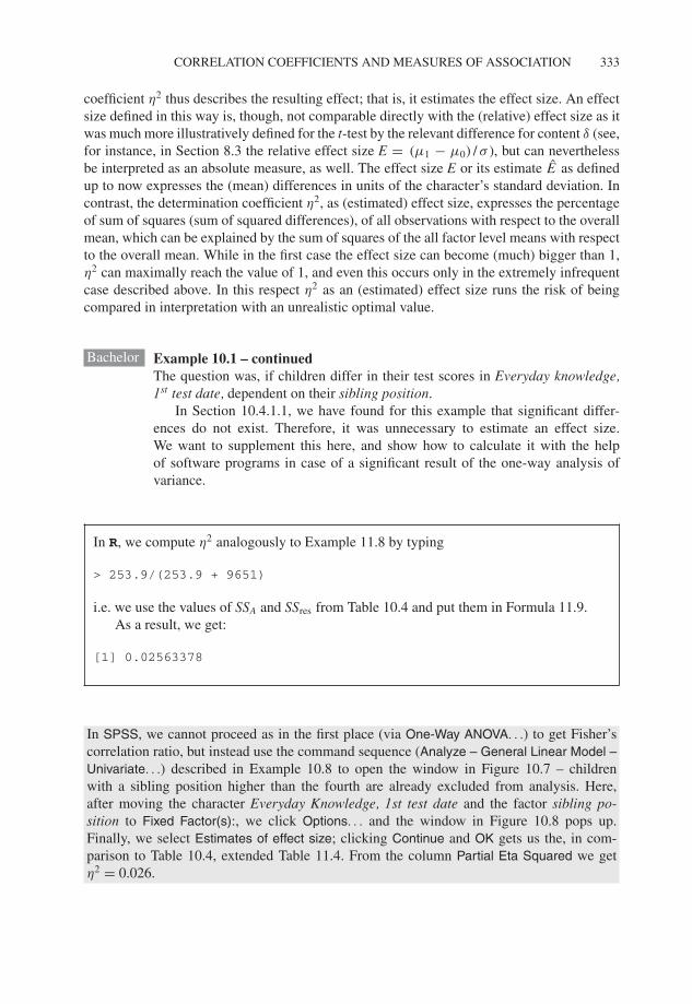
Bachelor Example 10.1 – continuedThe question was, if children differ in their test scores in Everyday knowledge,1st test date, dependent on their sibling position.
In Section 10.4.1.1, we have found for this example that significant differ-ences do not exist. Therefore, it was unnecessary to estimate an effect size.We want to supplement this here, and show how to calculate it with the helpof software programs in case of a significant result of the one-way analysis ofvariance.
In R, we compute η2 analogously to Example 11.8 by typing
> 253.9/(253.9 + 9651)
i.e. we use the values of SSA and SSres from Table 10.4 and put them in Formula 11.9.As a result, we get:
[1] 0.02563378
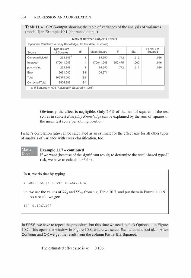
In SPSS, we cannot proceed as in the first place (via One-Way ANOVA. . .) to get Fisher’scorrelation ratio, but instead use the command sequence (Analyze – General Linear Model –Univariate. . .) described in Example 10.8 to open the window in Figure 10.7 – childrenwith a sibling position higher than the fourth are already excluded from analysis. Here,after moving the character Everyday Knowledge, 1st test date and the factor sibling po-sition to Fixed Factor(s):, we click Options. . . and the window in Figure 10.8 pops up.Finally, we select Estimates of effect size; clicking Continue and OK gets us the, in com-parison to Table 10.4, extended Table 11.4. From the column Partial Eta Squared we getη2 = 0.026.
P1: OTA/XYZ P2: ABCJWST094-c11 JWST094-Rasch September 22, 2011 16:25 Printer Name: Yet to Come
334 REGRESSION AND CORRELATION
Table 11.4 SPSS-output showing the table of variances of the analysis of variances(model I) in Example 10.1 (shortened output).
Partial EtaSquaredSig.FMean Squaredf
Type III Sumof Squares
Corrected Model
Intercept
pos_sibling
Error
Total
Corrected Total 919904.989
92263375.000
109.671889651.040
.026.513.77284.6503253.949
.946.0001550.475170041.9461170041.946
.026.513.77284.6503253.949a
Source
Tests of Between-Subjects Effects
Dependent Variable:Everyday Knowledge, 1st test date (T-Scores)
a. R Squared = .026 (Adjusted R Squared = -.008)
Obviously, the effect is negligible. Only 2.6% of the sum of squares of the testscores in subtest Everyday Knowledge can be explained by the sum of squares ofthe mean test score per sibling position.
Fisher’s correlation ratio can be calculated as an estimate for the effect size for all other typesof analysis of variance with cross classification, too.
MasterDoctor
Example 11.7 – continuedIf we want (because of the significant result) to determine the result-based type-IIrisk, we have to calculate η2 first.
In R, we do that by typing
> 386.392/(386.392 + 3247.474)
i.e. we use the values of SSA and SSres from e.g. Table 10.7, and put them in Formula 11.9.As a result, we get:
[1] 0.1063308
In SPSS, we have to repeat the procedure, but this time we need to click Options. . . in Figure10.7. This opens the window in Figure 10.8, where we select Estimates of effect size. AfterContinue and OK we get the result from the column Partial Eta Squared.
The estimated effect size is η2 = 0.106.
P1: OTA/XYZ P2: ABCJWST094-c11 JWST094-Rasch September 22, 2011 16:25 Printer Name: Yet to Come
CORRELATION COEFFICIENTS AND MEASURES OF ASSOCIATION 335
MasterDoctor
As opposed to the calculation according to Formula (11.9), in SPSS a ‘partial’ η2
is calculated as an estimated effect size in analysis of variance; in the case of one-way analysis of variance, this effect size coincides with η2. The underlying ideais to estimate, in the case of multi-way analyses of variance, the separated effectfor each case, when the corresponding null hypothesis is rejected. For instance,for the two-way analysis of variance of Table 10.10, the following three measuresof partial coefficients result:
η2A = SSA
SSA + SSres, η2
B = SSB
SSB + SSres, and η2
AB = SSAB
SSAB + SSres
So, for all partial coefficients we have η2part ≥ η2. Thus, the not very illustrative
interpretation of partial η2 is: the corresponding percentage of variance (to beformally correct: sum of squares) of all observations of the character of interest– corrected by the other factors’ contribution, the interaction effects included –which is explained by the variance (to be formally correct: sum of squares) of thefactor level means.
The ostensible advantage of estimation of the specific effect by the effect sizeof partial η2 is accompanied by the problem that, unlike for η2, the sum of allestimated effect sizes does not equal 1.
Referring to analysis of variance, the question of hypothesis testing concerning Fisher’scorrelation ratio has also been solved, and herewith also the question of planning a study.
11.3.5 Correlation between two nominal-scaled characters
In the case of relationships between two nominal-scaled characters, we have to distinguishgenerally between the case of both characters being dichotomous on one hand and the caseof at least one character being multi-categorical on the other hand.
In any case, the observation pairs (xv, yv) can be represented very clearly in a contingencytable, as we already did in previous chapters (see mainly Section 9.2.3); more exactly speaking,we talk about a two-dimensional contingency table, because two characters are given.
In the more general case, the character which was modeled by the random variable xhas r different categories, and the character modeled by y possesses c categories. Whenarranged in a matrix (table), r × c cells result, for example r rows times c columns. Thenumber of observed combinations of categories is entered in these cells. If n research unitsare given, the frequency per combination of categories is described by nij, i = 1, 2, . . . , r andj = 1, 2, . . . , c. The special case of r = c = 2 is of course included here. In this case, the tableis often referred to as a fourfold table or 2 × 2 table. In contrast, the general contingency tablethen is called an r × c table.
At first, we consider the general case with r > 2 and/or c > 2.If the number of categories r and number of categories c is not very big, any tendencies of
a relationship can be detected already from the contingency table. In doing so, it is importantto keep in mind that, because of the nominal-scaled categories, no direction of ‘arrangement oforder’ can be ascertained; all of the rows and all of the columns are generally interchangeablewith each other arbitrarily.
P1: OTA/XYZ P2: ABCJWST094-c11 JWST094-Rasch September 22, 2011 16:25 Printer Name: Yet to Come
336 REGRESSION AND CORRELATION
Bachelor Example 9.9 – continuedThe question was about the difference in marital status of the mother betweenchildren with German or Turkish as their native language. Using the χ2-test, wedetermined a significant difference. For this purpose we interpreted the characternative language of the child as a factor with the two factor levels ‘German’and ‘Turkish’. If a difference in the distribution on the categories of maritalstatus exists between children with German and children with Turkish as theirnative language, then a relationship between the two characters exists in so far ascertain categories of marital status occur more frequently and other categories lessfrequently in children whose native language is German then in children whosenative language is Turkish.
Table 9.5 shows mainly that children with Turkish as their native languagehave considerably more married mothers than the children with German as theirnative language. Contrariwise, the former have only a fraction of mothers withthe marital status ‘divorced’ compared to the latter.
The common measure for the general case of a contingency table is the so-called contingencycoefficient, more precisely Pearson’s contingency coefficient. Consequently, it is an unsignedmeasure and it is based on the statistic of the χ2-test from Formula (9.3):
C =√
χ2
χ2 + n
As it facilitates comprehension, we will use C for the statistic in the sample, and ζ for theparameter in the population, which is estimated by C; although this notation is not commonpractice. As this coefficient also cannot achieve the value of 1 in many cases, dependent onr · c, it is preferable to calculate (in the sample) the corrected contingency coefficient:
Ccorr =√
t
t − 1C (11.10)
in which t is the smaller of the two values r and c.
Bachelor Example 9.9 – continuedWe want to quantify the relationship determined by means of the χ2-test betweenmarital status of the mother and native language of the child.
In R, we apply the package vcd, which we load after its installation (see Chapter 1) usingthe function library(). Next, we type
> assoc.1 <- assocstats(table(marital_mother, native_language))> summary(assoc.1)
i.e. we create, using the function table(), a contingency table of the two charactersmarital status of the mother (marital_mother) and native language of the child(native_language), and submit it as an argument to the function assocstats();
P1: OTA/XYZ P2: ABCJWST094-c11 JWST094-Rasch September 22, 2011 16:25 Printer Name: Yet to Come
CORRELATION COEFFICIENTS AND MEASURES OF ASSOCIATION 337
the result of this analysis is assigned to the object assoc.1. Finally, we request thesummarized results with the function summary().
As a result, we get:
Number of cases in table: 100Number of factors: 2Test for independence of all factors:
Chisq = 16.463, df = 3, p-value = 0.0009112Chi-squared approximation may be incorrect
Xˆ2 df P(> Xˆ2)Likelihood Ratio 17.338 3 0.00060216Pearson 16.463 3 0.00091122
Phi-Coefficient : 0.406Contingency Coeff.: 0.376Cramer’s V : 0.406
To compute Ccorr we type
> sqrt(2/(2-1))*assoc.1$contingency
i.e. we conduct the computation according to Formula (11.10), and use the contingencycoefficient $contingency in the object assoc.1.
As a result, we get:
[1] 0.53171
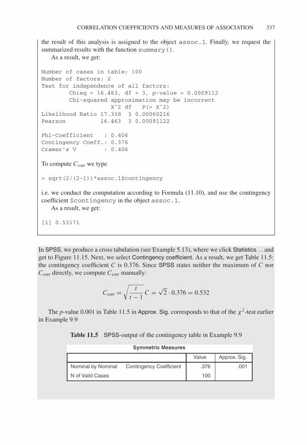
In SPSS, we produce a cross tabulation (see Example 5.13), where we click Statistics. . . andget to Figure 11.15. Next, we select Contingency coefficient. As a result, we get Table 11.5:the contingency coefficient C is 0.376. Since SPSS states neither the maximum of C norCcorr directly, we compute Ccorr manually:
Ccorr =√
t
t − 1C =
√2 · 0.376 = 0.532
The p-value 0.001 in Table 11.5 in Approx. Sig. corresponds to that of the χ2-test earlierin Example 9.9
Table 11.5 SPSS-output of the contingency table in Example 9.9
Approx. Sig.Value
Contingency Coefficient
N of Valid Cases
Nominal by Nominal
100
.001.376
Symmetric Measures
P1: OTA/XYZ P2: ABCJWST094-c11 JWST094-Rasch September 22, 2011 16:25 Printer Name: Yet to Come
338 REGRESSION AND CORRELATION
Compared to the maximum possible relationship, the observed relationshipbetween native language of the child and marital status of the mother is 53%;that is, a relationship of medium strength.
Other measures of association exist as well for this case, but they hardly play any role inpsychology (but see Kubinger, 1990). Nevertheless, some of them are output ‘automatically’by SPSS.
Doctor If, in the case of contingency tables, the question about the relationship betweentwo characters focuses on regression analysis, we generally have to differentiatebetween two models, as in analysis of variance. One of them is found only in-cidentally in psychology, but then mostly is simply not recognized at all by theresearcher as an entirely different statistical problem. The common case refers toresearch units being sampled by chance and for which the values in both char-acters have been ascertained accordingly (model II). In the other case (model I),one value per pair of outcomes (e.g. the value x) is determined or in other wordsselected in a systematic way, and only the corresponding y value is ascertainedaccordingly. An example for model I is the survey of Example 1.1 concerningthe children with German or Turkish as their native language: the researcherdetermined that 50 children from the first population and 50 children from thesecond population would be investigated. In this case, the values of x are not as-certained, but determined a priori. Therefore, the cases of application in Chapter9 differ from those in this chapter. There, the different rows (or columns, respec-tively) representing several populations have been determined with regard to theirmarginal totals prior to data acquisition; only the respective other marginal totalswere random. In the case examined here we have only one sample (of researchunits), and both marginal totals, of rows as well as of columns, are random. How-ever, this difference is of interest only theoretically: practically, the calculationprocedures for the association measures described here and for the χ2-test arethe same.
For Lecturers:
In contingency tables, a model III also exists; this is given in a famous exampleby Ronald A. Fisher (for more detailed information see e.g. Salsburg, 2002). Itis about an English lady who pretends to be able to find out in which order teaand milk had been put in a cup. Fisher designed an experiment, in which eightdifferent cups of tea were given to the lady for tasting, of which four were filled inone way and four cups in the other way. This was also told to the lady. Therewiththe marginal sums of, for instance, of the rows of the contingency table, are fixed.Given that the lady is intelligent, the marginal sums of the columns are also fixed,because the lady was told how many cups had been filled using each method ofpreparation.
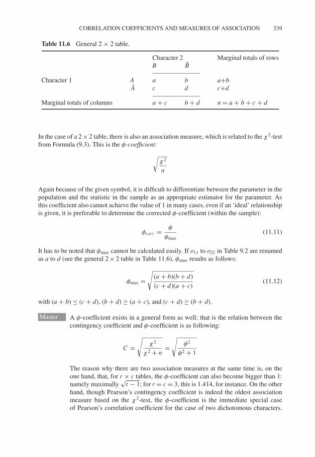
P1: OTA/XYZ P2: ABCJWST094-c11 JWST094-Rasch September 22, 2011 16:25 Printer Name: Yet to Come
CORRELATION COEFFICIENTS AND MEASURES OF ASSOCIATION 339
Table 11.6 General 2 × 2 table.
Character 2 Marginal totals of rowsB B
Character 1 A a b a+bA c d c+d
Marginal totals of columns a + c b + d n = a + b + c + d
In the case of a 2 × 2 table, there is also an association measure, which is related to the χ2-testfrom Formula (9.3). This is the φ-coefficient:
√χ2
n
Again because of the given symbol, it is difficult to differentiate between the parameter in thepopulation and the statistic in the sample as an appropriate estimator for the parameter. Asthis coefficient also cannot achieve the value of 1 in many cases, even if an ‘ideal’ relationshipis given, it is preferable to determine the corrected φ-coefficient (within the sample):
φcorr = φ
φmax(11.11)
It has to be noted that φmax cannot be calculated easily. If o11 to o22 in Table 9.2 are renamedas a to d (see the general 2 × 2 table in Table 11.6), φmax results as follows:
φmax =√
(a + b)(b + d)
(c + d)(a + c)(11.12)
with (a + b) ≤ (c + d), (b + d) ≥ (a + c), and (c + d) ≥ (b + d).
Master A φ-coefficient exists in a general form as well; that is the relation between thecontingency coefficient and φ-coefficient is as following:
C =√
χ2
χ2 + n=
√φ2
φ2 + 1
The reason why there are two association measures at the same time is, on theone hand, that, for r × c tables, the φ-coefficient can also become bigger than 1:namely maximally
√t − 1; for r = c = 3, this is 1.414, for instance. On the other
hand, though Pearson’s contingency coefficient is indeed the oldest associationmeasure based on the χ2-test, the φ-coefficient is the immediate special caseof Pearson’s correlation coefficient for the case of two dichotomous characters.
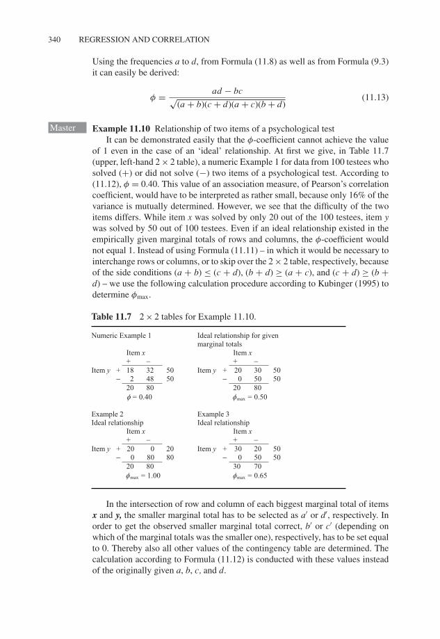
P1: OTA/XYZ P2: ABCJWST094-c11 JWST094-Rasch September 22, 2011 16:25 Printer Name: Yet to Come
340 REGRESSION AND CORRELATION
Using the frequencies a to d, from Formula (11.8) as well as from Formula (9.3)it can easily be derived:
φ = ad − bc√(a + b)(c + d)(a + c)(b + d)
(11.13)
Master Example 11.10 Relationship of two items of a psychological testIt can be demonstrated easily that the φ-coefficient cannot achieve the value
of 1 even in the case of an ‘ideal’ relationship. At first we give, in Table 11.7(upper, left-hand 2 × 2 table), a numeric Example 1 for data from 100 testees whosolved (+) or did not solve (−) two items of a psychological test. According to(11.12), φ = 0.40. This value of an association measure, of Pearson’s correlationcoefficient, would have to be interpreted as rather small, because only 16% of thevariance is mutually determined. However, we see that the difficulty of the twoitems differs. While item x was solved by only 20 out of the 100 testees, item ywas solved by 50 out of 100 testees. Even if an ideal relationship existed in theempirically given marginal totals of rows and columns, the φ-coefficient wouldnot equal 1. Instead of using Formula (11.11) – in which it would be necessary tointerchange rows or columns, or to skip over the 2 × 2 table, respectively, becauseof the side conditions (a + b) ≤ (c + d), (b + d) ≥ (a + c), and (c + d) ≥ (b +d) – we use the following calculation procedure according to Kubinger (1995) todetermine φmax.
Table 11.7 2 × 2 tables for Example 11.10.
Numeric Example 1 Ideal relationship for given marginal totals
Item x Item x + − + −
Item y + 18 32 50 Item y + 20 30 50 − 2 48 50 − 0 50 50
20 80 20 80 φ = 0.40 φ max = 0.50
Example 2 Ideal relationship
Example 3 Ideal relationship
Item x Item x + − + −
Item y + 20 0 20 Item y + 30 20 50 − 0 80 80 − 0 50 50
20 80 30 70 φ max = 1.00 φmax = 0.65
In the intersection of row and column of each biggest marginal total of itemsx and y, the smaller marginal total has to be selected as a′ or d′, respectively. Inorder to get the observed smaller marginal total correct, b′ or c′ (depending onwhich of the marginal totals was the smaller one), respectively, has to be set equalto 0. Thereby also all other values of the contingency table are determined. Thecalculation according to Formula (11.12) is conducted with these values insteadof the originally given a, b, c, and d.
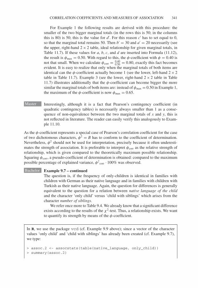
P1: OTA/XYZ P2: ABCJWST094-c11 JWST094-Rasch September 22, 2011 16:25 Printer Name: Yet to Come
CORRELATION COEFFICIENTS AND MEASURES OF ASSOCIATION 341
For Example 1 the following results are derived with this procedure: thesmaller of the two bigger marginal totals (in the rows this is 50; in the columnsthis is 80) is 50; this is the value for d′. For this reason c′ has to set equal to 0,so that the marginal total remains 50. Then b′ = 30 and a′ = 20 necessarily (seethe upper, right-hand 2 × 2 table, ideal relationship for given marginal totals, inTable 11.7). If these values for a, b, c, and d are inserted into Formula (11.12),the result is φmax = 0.50. With regard to this, the φ-coefficient with φ = 0.40 isnot that small. When we calculate φcorr = 0.40
0.50 = 0.80, exactly this fact becomesevident. It is easy to realize that only when the marginal totals of both items areidentical can the φ-coefficient actually become 1 (see the lower, left-hand 2 × 2table in Table 11.7). Example 3 (see the lower, right-hand 2 × 2 table in Table11.7) illustrates additionally that the φ-coefficient can become bigger the moresimilar the marginal totals of both items are: instead of φmax = 0.50 in Example 1,the maximum of the φ-coefficient is now φmax = 0.65.
Master Interestingly, although it is a fact that Pearson’s contingency coefficient (inquadratic contingency tables) is necessarily always smaller than 1 as a conse-quence of non-equivalence between the two marginal totals of x and y, this isnot reflected in literature. The reader can easily verify this analogously to Exam-ple 11.10.
As the φ-coefficient represents a special case of Pearson’s correlation coefficient for the caseof two dichotomous characters, φ2 = B has to conform to the coefficient of determination.Nevertheless, φ2 should not be used for interpretation, precisely because it often underesti-mates the strength of association. It is preferable to interpret φcorr as the relative strength ofrelationship, which is given compared to the theoretically maximum possible relationship.Squaring φcorr, a pseudo-coefficient of determination is obtained: compared to the maximumpossible percentage of explained variance, φ2
corr · 100% was observed.
Bachelor Example 9.7 – continuedThe question is, if the frequency of only-children is identical in families withchildren with German as their native language and in families with children withTurkish as their native language. Again, the question for differences is generallyequivalent to the question for a relation between native language of the childand the character ‘only child’ versus ‘child with siblings’ which arises from thecharacter number of siblings.
We refer once more to Table 9.4. We already know that a significant differenceexists according to the results of the χ2-test. Thus, a relationship exists. We wantto quantify its strength by means of the φ-coefficient.
In R, we use the package vcd (cf. Example 9.9 above); since a vector of the charactervalues ‘only child’ and ‘child with siblings’ has already been created (cf. Example 9.7),we type:
> assoc.2 <- assocstats(table(native_language, only_child))> summary(assoc.2)
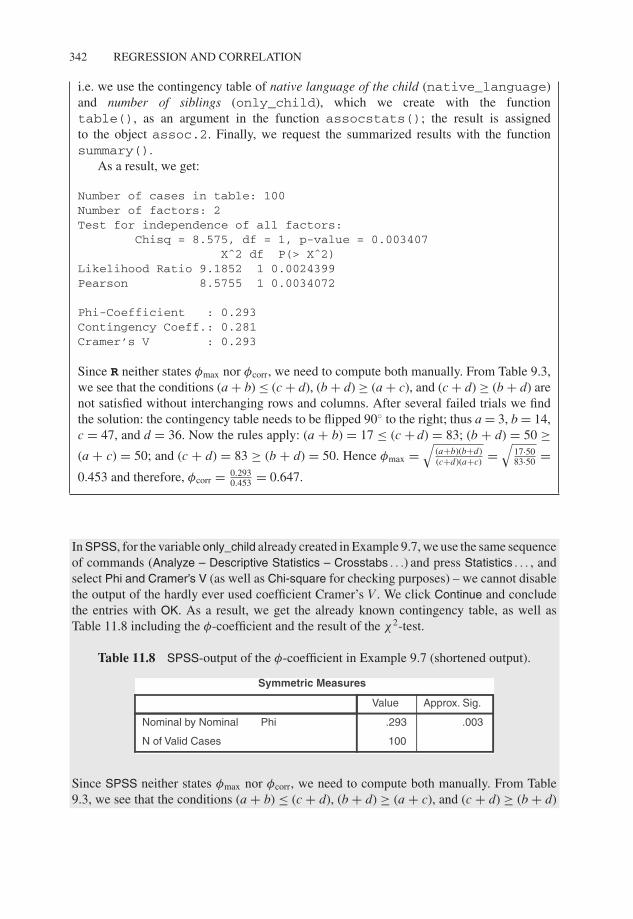
P1: OTA/XYZ P2: ABCJWST094-c11 JWST094-Rasch September 22, 2011 16:25 Printer Name: Yet to Come
342 REGRESSION AND CORRELATION
i.e. we use the contingency table of native language of the child (native_language)and number of siblings (only_child), which we create with the functiontable(), as an argument in the function assocstats(); the result is assignedto the object assoc.2. Finally, we request the summarized results with the functionsummary().
As a result, we get:
Number of cases in table: 100Number of factors: 2Test for independence of all factors:
Chisq = 8.575, df = 1, p-value = 0.003407Xˆ2 df P(> Xˆ2)
Likelihood Ratio 9.1852 1 0.0024399Pearson 8.5755 1 0.0034072
Phi-Coefficient : 0.293Contingency Coeff.: 0.281Cramer’s V : 0.293
Since R neither states φmax nor φcorr, we need to compute both manually. From Table 9.3,we see that the conditions (a + b) ≤ (c + d), (b + d) ≥ (a + c), and (c + d) ≥ (b + d) arenot satisfied without interchanging rows and columns. After several failed trials we findthe solution: the contingency table needs to be flipped 90◦ to the right; thus a = 3, b = 14,c = 47, and d = 36. Now the rules apply: (a + b) = 17 ≤ (c + d) = 83; (b + d) = 50 ≥(a + c) = 50; and (c + d) = 83 ≥ (b + d) = 50. Hence φmax =
√(a+b)(b+d)(c+d)(a+c) =
√17·5083·50 =
0.453 and therefore, φcorr = 0.2930.453 = 0.647.
In SPSS, for the variable only_child already created in Example 9.7, we use the same sequenceof commands (Analyze – Descriptive Statistics – Crosstabs . . .) and press Statistics . . . , andselect Phi and Cramer’s V (as well as Chi-square for checking purposes) – we cannot disablethe output of the hardly ever used coefficient Cramer’s V . We click Continue and concludethe entries with OK. As a result, we get the already known contingency table, as well asTable 11.8 including the φ-coefficient and the result of the χ2-test.
Table 11.8 SPSS-output of the φ-coefficient in Example 9.7 (shortened output).
Approx. Sig.Value
Phi
N of Valid Cases
Nominal by Nominal
100
.003.293
Symmetric Measures
Since SPSS neither states φmax nor φcorr, we need to compute both manually. From Table9.3, we see that the conditions (a + b) ≤ (c + d), (b + d) ≥ (a + c), and (c + d) ≥ (b + d)
P1: OTA/XYZ P2: ABCJWST094-c11 JWST094-Rasch September 22, 2011 16:25 Printer Name: Yet to Come
CORRELATION COEFFICIENTS AND MEASURES OF ASSOCIATION 343
are not satisfied without interchanging rows and columns. After several failed trials we findthe solution: the contingency table needs to be flipped 90◦ to the right; thus a = 3, b = 14,c = 47, and d = 36. Now the rules apply: (a + b) = 17 ≤ (c + d) = 83; (b + d) = 50 ≥(a + c) = 50; and (c + d) = 83 ≥ (b + d) = 50. Hence φmax =
√(a+b)(b+d)(c+d)(a+c) =
√17·5083·50 =
0.453 and therefore, φcorr = 0.2930.453 = 0.647.
The strength of the relationship, compared to the maximum possible relationship(for the given marginal totals), comes up to 64.7%. The calculated strength ofrelationship is considerable: children with Turkish as their native language areonly-children much less frequently than children with German as their nativelanguage. Squaring φcorr, we obtain a pseudo-coefficient of determination of0.6472 = 0.419. Compared to the maximum possible percentage of variance, weobserved 41.9%.
Referring to the χ2-test, the topic of hypothesis testing concerning relationships of twocharacters – given the corresponding scaling of the characters – is completed as well: thetest statistic in Formula (9.3) is valid for any two multi-categorical characters. Then, the nullhypothesis is, expanding or supplementary to Section 9.2.3 (with H0: p1j = p2j for all j) in thecase of an r × c contingency table, H0: phj = pgj for all j and all h and g (or, equivalently,H0: phj = phl for all h and all j and l) or now H0: ζ = 0, with the alternative hypothesis HA:phj �= pgj, for at least one j and h �= g (or, equivalently, HA: phj �= phl for at least one h andj �= l) or now HA: ζ > 0. For the φ-coefficient the same is true analogously; we just cannotdifferentiate between statistics and parameters in this case.
Contrariwise, with the reference of χ2-tests to measures of association, there is thepossibility to define a corresponding effect size and to estimate it for the case that the research
was not planned. Thus, if any χ2-distributed statistic is given, because of φ =√
χ2
n , in addition
to Fisher’s correlation ratio η2 is a further association- or correlation-based effect size that canbe estimated: φ2 = χ2 / n. However, interpretation is difficult, because, as described above,φ2 often cannot achieve the value of 1 even in cases of optimal explanation of variance due tothe given distributions of marginal totals. By the way, the (estimated) effect size φ2 is suitedgenerally as well for all standard normal-distributed statistics. As known from mathematicalstatistics, the squared standard normal-distributed z2 is χ2-distributed with df = 1 degreeof freedom. From that point of view the following effect size can be estimated as well:φ2 = z2 / n.
A particular question regarding the association of two nominal-scaled characters concernsthe concordance of two raters with respect to a certain character. In psychology, mainly inpsychological assessment, this is very frequently of interest, for instance with regard to theobjectivity of psychological testing or that is to say with regard to test administrator (examiner)effects (see Section 2.3). Somewhat misleadingly, one then talks about inter-rater reliability.It can be quantified by means of the kappa coefficient. This coefficient corrects the percentageof observed concordances over all categories by that percentage of accordance which wouldbe expected to occur in random ratings. Additionally, the resulting percentage is related to themaximum possible percentage which cannot be explained by chance. Using the notation for
P1: OTA/XYZ P2: ABCJWST094-c11 JWST094-Rasch September 22, 2011 16:25 Printer Name: Yet to Come
344 REGRESSION AND CORRELATION
the absolute frequencies in a quadratic contingency table (with r = c) such as, for example,in Section 9.2.3, and n = ∑c
i
∑cj oi j , this results in:
κ =
c∑
i=1
oii
n−
c∑
i=1
⎛
⎜⎜⎜⎝
c∑
j=1oi j
n
⎞
⎟⎟⎟⎠
⎛
⎜⎜⎜⎝
c∑
j=1o ji
n
⎞
⎟⎟⎟⎠
1 −c∑
i=1
⎛
⎜⎜⎜⎝
c∑
j=1oi j
n
⎞
⎟⎟⎟⎠
⎛
⎜⎜⎜⎝
c∑
j=1o ji
n
⎞
⎟⎟⎟⎠
(11.14)
In pertinent program packages even a test statistic for testing the null hypothesis H0: κ = 0(against the alternative hypothesis HA: κ > 0) is calculated; this test statistic is asymptoti-cally normally distributed. However, in applying the kappa coefficient one aims only for adescription of how close it comes to the ideal value of κ = 1, thus a complete concordance.
Bachelor Example 11.11 How strong is the concordance between two raters in an assess-ment center?
Within an assessment center, 25 participants in a seminar are rated by twoassessors with respect to their competence in a presentation exercise, accordingto three criteria: ‘convinces by content’ (1); ‘seems to be respectable, but doesnot convince by content’ (2); and ‘seems to be incompetent’ (3). The exact resultsare the following (ratings which are listed one upon the other stem from the sameparticipant. See Chapter 1 for the availability of the data):
Assessor 1 1 2 2 1 1 2 2 1 2 1 1 3 1 1 1 1 1 2 1 3 2 1 2 1 1Assessor 2 1 2 3 1 2 2 1 1 1 1 1 2 1 1 1 2 1 1 1 3 2 1 1 1 1
In R, we type
> assess1 <- c(1, 2, 2, 1, 1, 2, 2, 1, 2, 1, 1, 3, 1, 1, 1, 1,+ 1, 2, 1, 3, 2, 1, 2, 1, 1)> assess2 <- c(1, 2, 3, 1, 2, 2, 1, 1, 1, 1, 1, 2, 1, 1, 1, 2,+ 1, 1, 1, 3, 2, 1, 1, 1, 1)
i.e. we define the single values of each assessor as a separate vector by using the functionc(), and assign them to the objects assess1 and assess2, respectively. Next, we usethe appropriate function in the package vcd, namely
> Kappa(table(assess1, assess2))
i.e. we use assess1 and assess2 as arguments in the function table() to create acontingency table, which we submit as an argument to the function Kappa().
P1: OTA/XYZ P2: ABCJWST094-c11 JWST094-Rasch September 22, 2011 16:25 Printer Name: Yet to Come
CORRELATION COEFFICIENTS AND MEASURES OF ASSOCIATION 345
As a result, we get (shortened output):
Unweighted 0.3710692
In SPSS, we open a new data sheet (File – New – Data) and begin by typing in the twocharacters assess1 and assess2 according to the values above. Following the commandsequence (Analyze – Descriptive Statistics – Crosstabs. . .), we create a cross tabulationand use the character assess1 in the field Row(s): and the character assess2 in the fieldColumn(s):. By clicking Statistics. . . we open the window in Figure 8.11 (cf. Example 8.14),where we select Kappa, Continue, and confirm with OK. The result is κ = 0.371.
Compared to the maximum possible strength of concordance, the two assessorsconform to each other to 37.1%.
11.3.6 Nonlinear relationship in quantitative characters
In the case that the regression function f in (11.1) is plausibly not linear, a polynomialregression function – namely quadratic regression function – or logistic regression functioncomes into consideration.
Doctor The quadratic regression function is a polynomial of degree two. The correspond-ing regression model is
yv = β0 + β1xv + β2x2v + ev (11.15)
While the quadratic regression function is appropriate (better than the linear one)when the slope of the function is steeper in smaller values of x than in medium-sized values, and flatter for high values of x, the logistic regression function isappropriate when an inflection point exists in the course of the relation betweenx and y. The logistic regression results in the regression model
yv = β0
1 + β1eβ2 xv+ ev with β0, β1, β2 �= 0 (11.16)
Here β0 indicates the asymptotic value of yv, thus at the point where xv → ∞; β1
indicates the shift along the abscissa, and β2 the extent of curvature.
Doctor Example 11.12 Numeric example for quadratic and logistic regression functionswithout regard to content
We use the analysis of Example 11.5. This is about the relationship betweenthe character Applied Computing, 1st test date and Applied Computing, 2nd testdate. We would like to represent the scatter plot including a linear, a quadratic,and a logistic regression function.
P1: OTA/XYZ P2: ABCJWST094-c11 JWST094-Rasch September 22, 2011 16:25 Printer Name: Yet to Come
346 REGRESSION AND CORRELATION
In R, we type
> lm.lin <- lm(sub3_t2 ˜ sub3_t1)> lm.quad <- lm(sub3_t2 ˜ 1 + sub3_t1 + I(sub3_t1ˆ2))> nls.log <- nls(sub3_t2 ˜ SSlogis(sub3_t1, Asym, xmid, scal))
i.e. we use the function lm() to create regression models for the linear, the quadratic, andthe logistic regression function, respectively. Applied Computing, 1st test date (sub3_t1)is the regressor; Applied Computing, 2nd test date (sub3_t2) is the regressand. We spec-ify the linear regression function with sub3_t2 ˜ sub3_t1, and the quadratic withsub3_t2 ˜ 1 + sub3_t1 + I(sub3_t1ˆ2) – where the statement in I() rep-resents the quadratic term. In order to create the logistic regression function, we usethe function nls() in R with sub3_t2 ˜ SSlogis(sub3_t1, Asym, xmid,scal) – where the statement in SSlogis() represents the logistic term. The re-sulting regression models from the function lm() and nls() are assigned to the ob-jects lm.lin, lm.quad, and nls.log. Next we illustrate the scatter plot; therefore,we type
> plot(sub3_t1, sub3_t2,+ xlab = "Applied Computing, 1st test date (T-Scores)",+ ylab = "Applied Computing, 2nd test date (T-Scores)")
i.e. we use sub3_t1 and sub3_t2 as arguments in the function plot() and label theaxis with xlab and ylab. We add the regression functions to the chart, by typing
> abline(lm.lin)> lines(seq(35, 75, 0.1), predict(lm.quad,+ newdata = data.frame(sub3_t1 = seq(35, 75, 0.1))), lty = 5)> lines(seq(35,75, 0.1), predict(nls.log,+ newdata = data.frame(sub3_t1 = seq(35, 75, 0.1))), lty = 4)> legend("bottomright", lty = c(1, 5, 4),+ c("Linear", "Quadratic", "Logistic"))
i.e. we submit the linear regression function in the object lm.lin as an argument tothe function abline(). The function lines() draws a line using the coordinatesfrom the first argument, a number series from 35 to 75 in steps of 0.1 produced by thefunction seq(), and the second argument, the corresponding predicted values (newdata= data.frame) of the quadratic regression function in the object lm.quad using thefunction predict(); we proceed analogously for the logistic function. In doing so, wepredict the values of the character Applied Computing, 2nd test date from the possiblevalues 35 to 75 of the character Applied Computing, 1st test date (sub3_t1); withlty = 5 and lty = 4 we select the line types. Lastly, we create a legend(),set its position with the first argument, in this case the lower right corner of the chart("bottomright"), and amend it with the labels "Linear", "Quadratic", and"Logistic" using the function c().
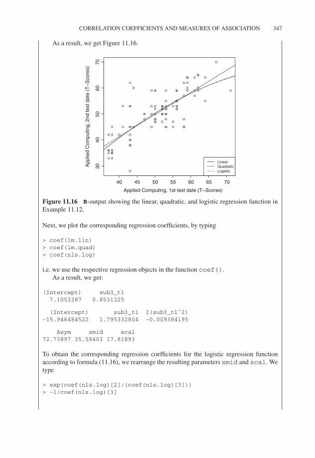
P1: OTA/XYZ P2: ABCJWST094-c11 JWST094-Rasch September 22, 2011 16:25 Printer Name: Yet to Come
CORRELATION COEFFICIENTS AND MEASURES OF ASSOCIATION 347
As a result, we get Figure 11.16.
40 45 50 55 60 65 70
3040
5060
70
Applied Computing, 1st test date (T−Scores)
App
lied
Com
putin
g, 2
nd te
st d
ate
(T−
Sco
res)
LinearQuadraticLogistic
Figure 11.16 R-output showing the linear, quadratic, and logistic regression function inExample 11.12.
Next, we plot the corresponding regression coefficients, by typing
> coef(lm.lin)> coef(lm.quad)> coef(nls.log)
i.e. we use the respective regression objects in the function coef().As a result, we get:
(Intercept) sub3_t17.1053387 0.8531325
(Intercept) sub3_t1 I(sub3_t1ˆ2)-15.946484522 1.795332804 -0.009384195
Asym xmid scal72.73897 35.58403 17.81893
To obtain the corresponding regression coefficients for the logistic regression functionaccording to formula (11.16), we rearrange the resulting parameters xmid and scal. Wetype
> exp(coef(nls.log)[2]/(coef(nls.log)[3]))> -1/coef(nls.log)[3]
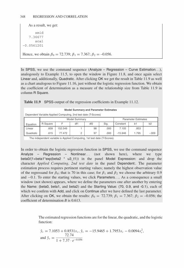
P1: OTA/XYZ P2: ABCJWST094-c11 JWST094-Rasch September 22, 2011 16:25 Printer Name: Yet to Come
348 REGRESSION AND CORRELATION
As a result, we get:
xmid7.36677
scal-0.0561201
Hence, we obtain β0 = 72.739; β1 = 7.367; β2 = –0.056.
In SPSS, we use the command sequence (Analyze – Regression – Curve Estimation. . .),analogously to Example 11.5, to open the window in Figure 11.8, and once again selectLinear and, additionally, Quadratic. After clicking OK we get the result in Table 11.9 as wellas a chart analogous to Figure 11.16, just without the logistic regression function. We obtainthe coefficient of determination as a measure of the relationship size from Table 11.9 incolumn R Square.
Table 11.9 SPSS-output of the regression coefficients in Example 11.12.
Sig.df2df1FR Square b2b1Constant
Parameter EstimatesModel Summary
Linear
Quadratic -.0091.795-15.946.00097277.472.615
.8537.105.000981152.549.609
Equation
Model Summary and Parameter Estimates
The independent variable is Applied Computing, 1st test date (T-Scores).
Dependent Variable:Applied Computing, 2nd test date (T-Scores)
In order to obtain the logistic regression function in SPSS, we use the command sequenceAnalyze – Regression – Nonlinear. . . (not shown here), where we typebeta0/(1+beta1*exp(beta2 * u3_t1)) in the panel Model Expression: and drop thecharacter Applied Computing, 2nd test date in the panel Dependent:. The parameterestimation process requires pertinent starting values; namely the highest observation valueof the regressand for β0; that is 70 in this case; for β1 and β2 we choose the arbitrary 0.9and −0.1. To enter the starting values, we click Parameters. . .. As a consequence a smallwindow (not shown) appears, where we define the parameters one after another by enteringthe Name: (beta0, beta1, and beta2) and the Starting Value: (70, 0.9, and -0.1), each ofwhich we confirm with Add, and click on Continue after we have defined the last parameter.After clicking on OK, we obtain the results: β0 = 72.739; β1 = 7.367; β2 = –0.056; thecoefficient of determination B is 0.613.
The estimated regression functions are for the linear, the quadratic, and the logisticfunction:
yv = 7.1053 + 0.8531xv , yv = −15.9465 + 1.7953xv − 0.0094x2v ,
and yv = 72.74
1 + 7.37 · e−0.056
P1: OTA/XYZ P2: ABCJWST094-c11 JWST094-Rasch September 22, 2011 16:25 Printer Name: Yet to Come
HYPOTHESIS TESTING AND PLANNING THE STUDY 349
We recognize that the linear regression describes the data hardly any worse thando the two selected nonlinear regressions; see Chapter 14 for more details.
11.4 Hypothesis testing and planning the study concerningcorrelation coefficients
We have described the methods of regression and correlation mainly for the purpose ofdescriptive statistics, so far. However, when dealing with the regression model (and Pearson’scorrelation coefficient), the difference between the result in the sample and the true relationshipin the corresponding population already has been denoted. Naturally, as for the case of justone character, in inferential statistics the subjects of (point) estimation, confidence intervals,and hypothesis testing, and (mainly with respect to the last of these), planning of the studyand sequential testing, become relevant.
The point estimator for Pearson’s correlation coefficient has already been discussed above(see Formula (11.8)), and actually also the one for regression coefficients by explicitly indicat-ing the estimates in Formulas (11.5) and (11.6). For the association measures discussed here,it was addressed at least implicitly that the statistics from the sample yield point estimates forthe underlying parameters. Similarly, the calculated correlation coefficients for ordinal-scaledcharacters are to be regarded as estimates. As for confidence intervals, most software packagesoutput standard errors, by means of which the user can generally calculate the confidenceintervals for β0 and β1. However, in psychological research the confidence interval for theparameters of a regression line is hardly of interest. The same applies to hypothesis testingwith regard to the parameters of the regression line and therewith also for the correspondingplanning of the study. In contrast, these subjects are important for Pearson’s correlation co-efficient in psychological research practice. They are discussed in detail in the following. Aswe remember, we have to assume that the two characters of interest, which are modeled byrandom variables, are normally distributed.
Doctor In Table 11.1 (or in the corresponding summary of results in the calculation withR, respectively) of Example 11.5, in addition to the regression coefficients for theexample (of which the content is not of interest here), after analysis conducted bymeans of SPSS, three supplementary columns can be found: the standard error,the value of a t-distributed statistic (whose formula we will not reproduce here),and the p-value. This last refers implicitly to the null hypotheses H0: β0 = 0and H0: β1 = 0, respectively. If the type-I risk has been determined by α =0.05 previously, then both null hypotheses have to be rejected. Using R, the sameinformation is obtained. For calculation of the confidence intervals for β0 and β1,the indicated standard error can be used. For β1 it corresponds to the term with thesquare root in the following formula for the lower limit L and the upper limit U:
L = b1 − t(
n − 2, 1 − α
2
) √1
n − 2
(s2
y
s2x
− b21
)
;
U = b1 + t(
n − 2, 1 − α
2
) √1
n − 2
(s2
y
s2x
− b21
)
(11.17)
P1: OTA/XYZ P2: ABCJWST094-c11 JWST094-Rasch September 22, 2011 16:25 Printer Name: Yet to Come
350 REGRESSION AND CORRELATION
The determination of a confidence interval for Pearson’s correlation coefficient is easilypossible with R; we do not explain the planning of the study with regard to the confi-dence interval here, because in psychological research the main focus is rather on hypothesistesting.
MasterDoctor
SPSS delivers a confidence interval for Pearson’s correlation coefficient via boot-strapping (see Section 14.4). An approximate confidence interval with the lowerlimit L and the upper limit U can be determined as follows:
L = 1
2ln
1 + r1 − r
−z(
1 − α
2
)
√n − 3
; U = 1
2ln
1 + r1 − r
+z(
1 − α
2
)
√n − 3
(11.18)
MasterDoctor
Example 11.13 How strong is the relationship between Everyday Knowledgeand Applied Computing (at the first test date) in Example 1.1?
We are not content to calculate a point estimate, but want to calculate aconfidence interval for ρ with a confidence coefficient of 1 – α = 0.95.
In R, we type
> cor.test(sub1_t1, sub3_t1, alternative = "two.sided",+ method = "pearson", conf.level = 0.95)
i.e. we use the two characters Everyday Knowledge, 1st test date (sub1_t1) and Ap-plied Computing, 1st test date (sub3_t1) as arguments in the function cor.test();with alternative = "two.sided" we select the two sided alternative hypothesisHA: ρ �= 0; with method = "pearson" we request the product-moment correlationcoefficient; and conf.level = 0.95 sets the confidence coefficient.
As a result, we get:
Pearson’s product-moment correlation
data: sub1_t1 and sub3_t1t = 4.7371, df = 98, p-value = 7.33e-06alternative hypothesis: true correlation is not equal to 095 percent confidence interval:0.2570199 0.5789775
sample estimates:cor
0.431647
For SPSS, we create a complementary syntax. We begin with the command sequence(Analyze – Correlate – Bivariate. . .) described in Example 11.6. The result is r = ρ = 0.432.Next, we open a new data sheet (File – New – Data) and, in the Variable View, define thecharacters r and n; then, we change to Data View and type the number 0.432 in the first
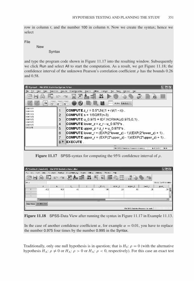
P1: OTA/XYZ P2: ABCJWST094-c11 JWST094-Rasch September 22, 2011 16:25 Printer Name: Yet to Come
HYPOTHESIS TESTING AND PLANNING THE STUDY 351
row in column r, and the number 100 in column n. Now we create the syntax; hence weselect
FileNew
Syntax
and type the program code shown in Figure 11.17 into the resulting window. Subsequentlywe click Run and select All to start the computation. As a result, we get Figure 11.18; theconfidence interval of the unknown Pearson’s correlation coefficient ρ has the bounds 0.26and 0.58.
Figure 11.17 SPSS-syntax for computing the 95% confidence interval of ρ.
Figure 11.18 SPSS-Data View after running the syntax in Figure 11.17 in Example 11.13.
In the case of another confidence coefficient α, for example α = 0.01, you have to replacethe number 0.975 four times by the number 0.995 in the Syntax.
Traditionally, only one null hypothesis is in question; that is H0: ρ = 0 (with the alternativehypothesis HA: ρ �= 0 or HA: ρ > 0 or HA: ρ < 0, respectively). For this case an exact test
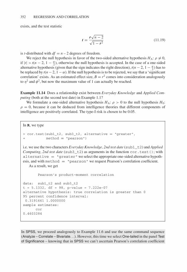
P1: OTA/XYZ P2: ABCJWST094-c11 JWST094-Rasch September 22, 2011 16:25 Printer Name: Yet to Come
352 REGRESSION AND CORRELATION
exists, and the test statistic
t = r√
n − 2√1 − r2
(11.19)
is t-distributed with df = n – 2 degrees of freedom.We reject the null hypothesis in favor of the two-sided alternative hypothesis HA: ρ �= 0,
if |t| > t(n − 2, 1 − α2 ), otherwise the null hypothesis is accepted. In the case of a one-sided
alternative hypothesis (given that the sign indicates the right direction), t(n − 2, 1 − α2 ) has to
be replaced by t(n − 2, 1 − α). If the null hypothesis is to be rejected, we say that a ‘significantcorrelation’ exists. As an estimated effect size, B = r2 comes into consideration analogouslyto η2 and φ2, but now the maximum value of 1 can actually be reached.
Example 11.14 Does a relationship exist between Everyday Knowledge and Applied Com-puting (both at the second test date) in Example 1.1?
We formulate a one-sided alternative hypothesis HA: ρ > 0 to the null hypothesis H0:ρ = 0, because it can be deduced from intelligence theories that different components ofintelligence are positively correlated. The type-I risk is chosen to be 0.05.
In R, we type
> cor.test(sub1_t2, sub3_t2, alternative = "greater",+ method = "pearson")
i.e. we use the two characters Everyday Knowledge, 2nd test date (sub1_t2) and AppliedComputing, 2nd test date (sub3_t2) as arguments in the function cor.test(); withalternative = "greater"we select the appropriate one-sided alternative hypoth-esis, and with method = "pearson" we request Pearson’s correlation coefficient.
As a result, we get
Pearson’s product-moment correlation
data: sub1_t2 and sub3_t2t = 5.1332, df = 98, p-value = 7.222e-07alternative hypothesis: true correlation is greater than 095 percent confidence interval:0.3191661 1.0000000
sample estimates:cor
0.4603284
In SPSS, we proceed analogously to Example 11.6 and use the same command sequence(Analyze – Correlate – Bivariate. . .). However, this time we select One-tailed in the panel Testof Significance – knowing that in SPSS we can’t ascertain Pearson’s correlation coefficient
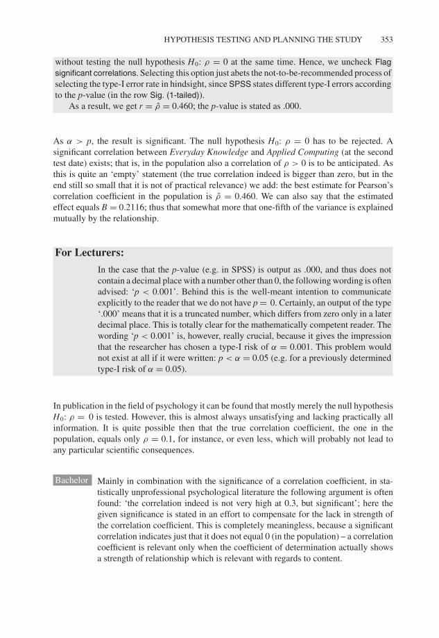
P1: OTA/XYZ P2: ABCJWST094-c11 JWST094-Rasch September 22, 2011 16:25 Printer Name: Yet to Come
HYPOTHESIS TESTING AND PLANNING THE STUDY 353
without testing the null hypothesis H0: ρ = 0 at the same time. Hence, we uncheck Flagsignificant correlations. Selecting this option just abets the not-to-be-recommended process ofselecting the type-I error rate in hindsight, since SPSS states different type-I errors accordingto the p-value (in the row Sig. (1-tailed)).
As a result, we get r = ρ = 0.460; the p-value is stated as .000.
As α > p, the result is significant. The null hypothesis H0: ρ = 0 has to be rejected. Asignificant correlation between Everyday Knowledge and Applied Computing (at the secondtest date) exists; that is, in the population also a correlation of ρ > 0 is to be anticipated. Asthis is quite an ‘empty’ statement (the true correlation indeed is bigger than zero, but in theend still so small that it is not of practical relevance) we add: the best estimate for Pearson’scorrelation coefficient in the population is ρ = 0.460. We can also say that the estimatedeffect equals B = 0.2116; thus that somewhat more that one-fifth of the variance is explainedmutually by the relationship.
For Lecturers:
In the case that the p-value (e.g. in SPSS) is output as .000, and thus does notcontain a decimal place with a number other than 0, the following wording is oftenadvised: ‘p < 0.001’. Behind this is the well-meant intention to communicateexplicitly to the reader that we do not have p = 0. Certainly, an output of the type‘.000’ means that it is a truncated number, which differs from zero only in a laterdecimal place. This is totally clear for the mathematically competent reader. Thewording ‘p < 0.001’ is, however, really crucial, because it gives the impressionthat the researcher has chosen a type-I risk of α = 0.001. This problem wouldnot exist at all if it were written: p < α = 0.05 (e.g. for a previously determinedtype-I risk of α = 0.05).
In publication in the field of psychology it can be found that mostly merely the null hypothesisH0: ρ = 0 is tested. However, this is almost always unsatisfying and lacking practically allinformation. It is quite possible then that the true correlation coefficient, the one in thepopulation, equals only ρ = 0.1, for instance, or even less, which will probably not lead toany particular scientific consequences.
Bachelor Mainly in combination with the significance of a correlation coefficient, in sta-tistically unprofessional psychological literature the following argument is oftenfound: ‘the correlation indeed is not very high at 0.3, but significant’; here thegiven significance is stated in an effort to compensate for the lack in strength ofthe correlation coefficient. This is completely meaningless, because a significantcorrelation indicates just that it does not equal 0 (in the population) – a correlationcoefficient is relevant only when the coefficient of determination actually showsa strength of relationship which is relevant with regards to content.
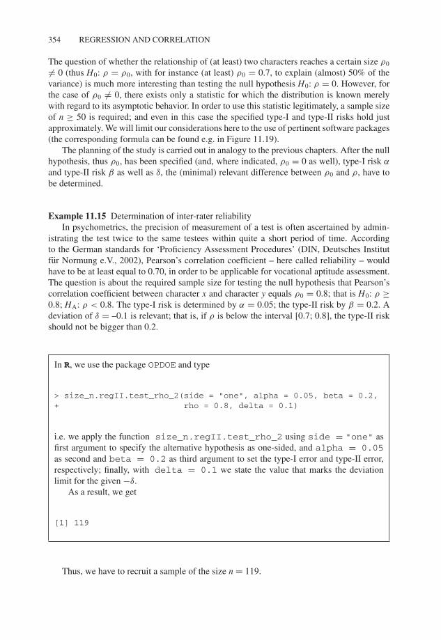
P1: OTA/XYZ P2: ABCJWST094-c11 JWST094-Rasch September 22, 2011 16:25 Printer Name: Yet to Come
354 REGRESSION AND CORRELATION
The question of whether the relationship of (at least) two characters reaches a certain size ρ0
�= 0 (thus H0: ρ = ρ0, with for instance (at least) ρ0 = 0.7, to explain (almost) 50% of thevariance) is much more interesting than testing the null hypothesis H0: ρ = 0. However, forthe case of ρ0 �= 0, there exists only a statistic for which the distribution is known merelywith regard to its asymptotic behavior. In order to use this statistic legitimately, a sample sizeof n ≥ 50 is required; and even in this case the specified type-I and type-II risks hold justapproximately. We will limit our considerations here to the use of pertinent software packages(the corresponding formula can be found e.g. in Figure 11.19).
The planning of the study is carried out in analogy to the previous chapters. After the nullhypothesis, thus ρ0, has been specified (and, where indicated, ρ0 = 0 as well), type-I risk α
and type-II risk β as well as δ, the (minimal) relevant difference between ρ0 and ρ, have tobe determined.
Example 11.15 Determination of inter-rater reliabilityIn psychometrics, the precision of measurement of a test is often ascertained by admin-
istrating the test twice to the same testees within quite a short period of time. Accordingto the German standards for ‘Proficiency Assessment Procedures’ (DIN, Deutsches Institutfur Normung e.V., 2002), Pearson’s correlation coefficient – here called reliability – wouldhave to be at least equal to 0.70, in order to be applicable for vocational aptitude assessment.The question is about the required sample size for testing the null hypothesis that Pearson’scorrelation coefficient between character x and character y equals ρ0 = 0.8; that is H0: ρ ≥0.8; HA: ρ < 0.8. The type-I risk is determined by α = 0.05; the type-II risk by β = 0.2. Adeviation of δ = –0.1 is relevant; that is, if ρ is below the interval [0.7; 0.8], the type-II riskshould not be bigger than 0.2.
In R, we use the package OPDOE and type
> size_n.regII.test_rho_2(side = "one", alpha = 0.05, beta = 0.2,+ rho = 0.8, delta = 0.1)
i.e. we apply the function size_n.regII.test_rho_2 using side = "one" asfirst argument to specify the alternative hypothesis as one-sided, and alpha = 0.05as second and beta = 0.2 as third argument to set the type-I error and type-II error,respectively; finally, with delta = 0.1 we state the value that marks the deviationlimit for the given −δ.
As a result, we get
[1] 119
Thus, we have to recruit a sample of the size n = 119.
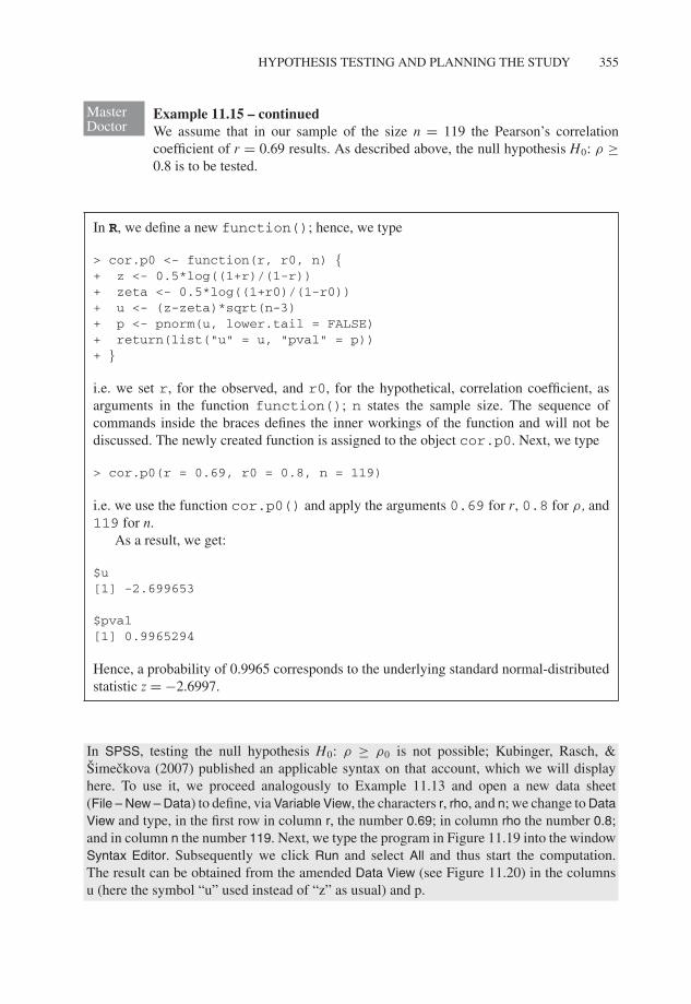
P1: OTA/XYZ P2: ABCJWST094-c11 JWST094-Rasch September 22, 2011 16:25 Printer Name: Yet to Come
HYPOTHESIS TESTING AND PLANNING THE STUDY 355
MasterDoctor
Example 11.15 – continuedWe assume that in our sample of the size n = 119 the Pearson’s correlationcoefficient of r = 0.69 results. As described above, the null hypothesis H0: ρ ≥0.8 is to be tested.
In R, we define a new function(); hence, we type
> cor.p0 <- function(r, r0, n) {+ z <- 0.5*log((1+r)/(1-r))+ zeta <- 0.5*log((1+r0)/(1-r0))+ u <- (z-zeta)*sqrt(n-3)+ p <- pnorm(u, lower.tail = FALSE)+ return(list("u" = u, "pval" = p))+ }
i.e. we set r, for the observed, and r0, for the hypothetical, correlation coefficient, asarguments in the function function(); n states the sample size. The sequence ofcommands inside the braces defines the inner workings of the function and will not bediscussed. The newly created function is assigned to the object cor.p0. Next, we type
> cor.p0(r = 0.69, r0 = 0.8, n = 119)
i.e. we use the function cor.p0() and apply the arguments 0.69 for r, 0.8 for ρ, and119 for n.
As a result, we get:
$u[1] -2.699653
$pval[1] 0.9965294
Hence, a probability of 0.9965 corresponds to the underlying standard normal-distributedstatistic z = −2.6997.
In SPSS, testing the null hypothesis H0: ρ ≥ ρ0 is not possible; Kubinger, Rasch, &Simeckova (2007) published an applicable syntax on that account, which we will displayhere. To use it, we proceed analogously to Example 11.13 and open a new data sheet(File – New – Data) to define, via Variable View, the characters r, rho, and n; we change to DataView and type, in the first row in column r, the number 0.69; in column rho the number 0.8;and in column n the number 119. Next, we type the program in Figure 11.19 into the windowSyntax Editor. Subsequently we click Run and select All and thus start the computation.The result can be obtained from the amended Data View (see Figure 11.20) in the columnsu (here the symbol “u” used instead of “z” as usual) and p.
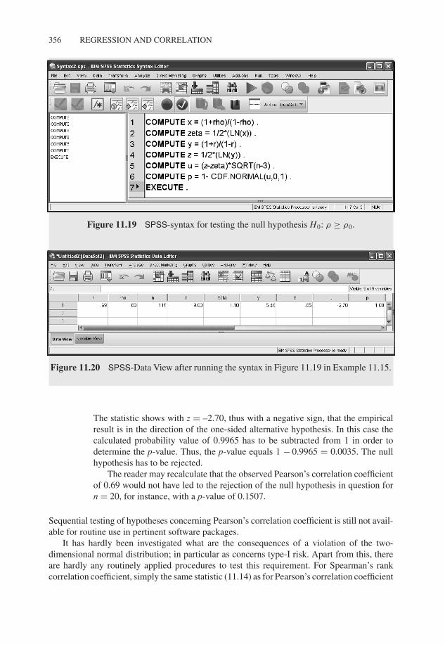
P1: OTA/XYZ P2: ABCJWST094-c11 JWST094-Rasch September 22, 2011 16:25 Printer Name: Yet to Come
356 REGRESSION AND CORRELATION
Figure 11.19 SPSS-syntax for testing the null hypothesis H0: ρ ≥ ρ0.
Figure 11.20 SPSS-Data View after running the syntax in Figure 11.19 in Example 11.15.
The statistic shows with z = –2.70, thus with a negative sign, that the empiricalresult is in the direction of the one-sided alternative hypothesis. In this case thecalculated probability value of 0.9965 has to be subtracted from 1 in order todetermine the p-value. Thus, the p-value equals 1 − 0.9965 = 0.0035. The nullhypothesis has to be rejected.
The reader may recalculate that the observed Pearson’s correlation coefficientof 0.69 would not have led to the rejection of the null hypothesis in question forn = 20, for instance, with a p-value of 0.1507.
Sequential testing of hypotheses concerning Pearson’s correlation coefficient is still not avail-able for routine use in pertinent software packages.
It has hardly been investigated what are the consequences of a violation of the two-dimensional normal distribution; in particular as concerns type-I risk. Apart from this, thereare hardly any routinely applied procedures to test this requirement. For Spearman’s rankcorrelation coefficient, simply the same statistic (11.14) as for Pearson’s correlation coefficient
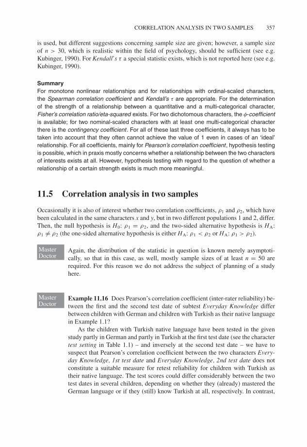
P1: OTA/XYZ P2: ABCJWST094-c11 JWST094-Rasch September 22, 2011 16:25 Printer Name: Yet to Come
CORRELATION ANALYSIS IN TWO SAMPLES 357
is used, but different suggestions concerning sample size are given; however, a sample sizeof n > 30, which is realistic within the field of psychology, should be sufficient (see e.g.Kubinger, 1990). For Kendall’s τ a special statistic exists, which is not reported here (see e.g.Kubinger, 1990).
SummaryFor monotone nonlinear relationships and for relationships with ordinal-scaled characters,the Spearman correlation coefficient and Kendall’s τ are appropriate. For the determinationof the strength of a relationship between a quantitative and a multi-categorical character,Fisher’s correlation ratio/eta-squared exists. For two dichotomous characters, the φ-coefficientis available; for two nominal-scaled characters with at least one multi-categorical characterthere is the contingency coefficient. For all of these last three coefficients, it always has to betaken into account that they often cannot achieve the value of 1 even in cases of an ‘ideal’relationship. For all coefficients, mainly for Pearson’s correlation coefficient, hypothesis testingis possible, which in praxis mostly concerns whether a relationship between the two charactersof interests exists at all. However, hypothesis testing with regard to the question of whether arelationship of a certain strength exists is much more meaningful.
11.5 Correlation analysis in two samples
Occasionally it is also of interest whether two correlation coefficients, ρ1 and ρ2, which havebeen calculated in the same characters x and y, but in two different populations 1 and 2, differ.Then, the null hypothesis is H0: ρ1 = ρ2, and the two-sided alternative hypothesis is HA:ρ1 �= ρ2 (the one-sided alternative hypothesis is either HA: ρ1 < ρ2 or HA: ρ1 > ρ2).
MasterDoctor
Again, the distribution of the statistic in question is known merely asymptoti-cally, so that in this case, as well, mostly sample sizes of at least n = 50 arerequired. For this reason we do not address the subject of planning of a studyhere.
MasterDoctor
Example 11.16 Does Pearson’s correlation coefficient (inter-rater reliability) be-tween the first and the second test date of subtest Everyday Knowledge differbetween children with German and children with Turkish as their native languagein Example 1.1?
As the children with Turkish native language have been tested in the givenstudy partly in German and partly in Turkish at the first test date (see the charactertest setting in Table 1.1) – and inversely at the second test date – we have tosuspect that Pearson’s correlation coefficient between the two characters Every-day Knowledge, 1st test date and Everyday Knowledge, 2nd test date does notconstitute a suitable measure for retest reliability for children with Turkish astheir native language. The test scores could differ considerably between the twotest dates in several children, depending on whether they (already) mastered theGerman language or if they (still) know Turkish at all, respectively. In contrast,
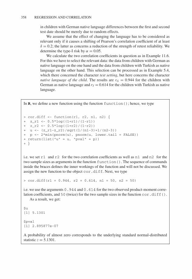
P1: OTA/XYZ P2: ABCJWST094-c11 JWST094-Rasch September 22, 2011 16:25 Printer Name: Yet to Come
358 REGRESSION AND CORRELATION
in children with German native language differences between the first and secondtest date should be merely due to random effects.
We assume that the effect of changing the language has to be considered asrelevant only if it causes a shifting of Pearson’s correlation coefficient of at leastδ = 0.2; the latter as concerns a reduction of the strength of retest reliability. Wedetermine the type-I risk by α = 0.05.
We calculate the two correlation coefficients in question as in Example 11.6.For this we have to select the relevant data: the data from children with German asnative language on the one hand and the data from children with Turkish as nativelanguage on the other hand. This selection can be processed as in Example 5.4,which there concerned the character test setting, but here concerns the characternative language of the child. The results are rG = 0.944 for the children withGerman as native language and rT = 0.614 for the children with Turkish as nativelanguage.
In R, we define a new function using the function function(); hence, we type
> cor.diff <- function(r1, r2, n1, n2) {+ z_r1 <- 0.5*log((1+r1)/(1-r1))+ z_r2 <- 0.5*log((1+r2)/(1-r2))+ u <- (z_r1-z_r2)/sqrt(1/(n1-3)+1/(n2-3))+ p <- 2*min(pnorm(u), pnorm(u, lower.tail = FALSE))+ return(list("u" = u, "pval" = p))+ }
i.e. we set r1 and r2 for the two correlation coefficients as well as n1 and n2 for thetwo sample sizes as arguments in the function function(). The sequence of commandsinside the braces defines the inner workings of the function and will not be discussed. Weassign the new function to the object cor.diff. Next, we type
> cor.diff(r1 = 0.944, r2 = 0.614, n1 = 50, n2 = 50)
i.e. we use the arguments 0.944 and 0.614 for the two observed product-moment corre-lation coefficients, and 50 (twice) for the two sample sizes in the function cor.diff().
As a result, we get:
$u[1] 5.1301
$pval[1] 2.895877e-07
A probability of almost zero corresponds to the underlying standard normal-distributedstatistic z = 5.1301.
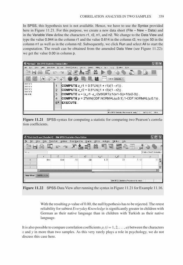
P1: OTA/XYZ P2: ABCJWST094-c11 JWST094-Rasch September 22, 2011 16:25 Printer Name: Yet to Come
CORRELATION ANALYSIS IN TWO SAMPLES 359
In SPSS, this hypothesis test is not available. Hence, we have to use the Syntax providedhere in Figure 11.21. For this purpose, we create a new data sheet (File – New – Data) andin the Variable View define the characters r1, r2, n1, and n2. We change to the Data View andtype the value 0.944 in the column r1 and the value 0.614 in the column r2; we type 50 in thecolumn n1 as well as in the column n2. Subsequently, we click Run and select All to start thecomputation. The result can be obtained from the amended Data View (see Figure 11.22):we get the value 0.00 in column p.
Figure 11.21 SPSS-syntax for computing a statistic for comparing two Pearson’s correla-tion coefficients.
Figure 11.22 SPSS-Data View after running the syntax in Figure 11.21 for Example 11.16.
With the resulting p-value of 0.00, the null hypothesis has to be rejected. The retestreliability for subtest Everyday Knowledge is significantly greater in children withGerman as their native language than in children with Turkish as their nativelanguage.
It is also possible to compare correlation coefficients ρ i (i = 1, 2, . . . , a) between the charactersx and y in more than two samples. As this very rarely plays a role in psychology, we do notdiscuss this case here.

P1: OTA/XYZ P2: ABCJWST094-c11 JWST094-Rasch September 22, 2011 16:25 Printer Name: Yet to Come
360 REGRESSION AND CORRELATION
References
DIN, Deutsches Institut fur Normung e.V. (2002). DIN 33430: Anforderungen an Verfahren und derenEinsatz bei berufsbezogenen Eignungsbeurteilungen. [Requirements for Proficiency Assessment Pro-cedures and Their Implementation]. Berlin: Beuth.
Kubinger, K. D. (1990). Ubersicht und Interpretation der verschiedenen Assoziationsmaße [Review ofmeasures of association]. Psychologische Beitrage, 32, 290–346.
Kubinger, K. D. (1995). Entgegnung: Zur Korrektur des φ-Koeffizienten [Riposte: On the correction ofthe φ-coefficient]. Newsletter der Fachgruppe Methoden in der deutschen Gesellschaft fur Psycholo-gie, 3, 3–4.
Kubinger, K. D., Rasch, D., & Simeckova, M. (2007). Testing a correlation coefficient’s significance:using H0: 0 < ρ ≤ λ is preferable to H0: ρ = 0. Psychology Science, 49, 74–87.
Rasch, D., Verdooren, L. R., & Gowers, J. I. (2007). Fundamentals in the Design and Analysis ofExperiments and Surveys (2nd edn). Munich: Oldenbourg.
Salsburg, D. (2002). The Lady Tasting Tea. New York: Owl Books.