statistical tools for analyzing water quality data · statistical tools for analyzing water quality...

0

Statistical Tools for Analyzing Water Quality Data

Liya Fu1 and You-Gan Wang2*

1School of Science, Xian Jiaotong University, China and Centre for Applications in NaturalResource Mathematics (CARM), School of Mathematics and Physics,

the University of Queensland2Centre for Applications in Natural Resource Mathematics (CARM), School of

Mathematics and Physics, The University of QueenslandAustralia

1. Introduction

Water quality data are often collected at different sites over time to improve waterquality management. Water quality data usually exhibit the following characteristics:non-normal distribution, presence of outliers, missing values, values below detection limits(censored), and serial dependence. It is essential to apply appropriate statistical methodologywhen analyzing water quality data to draw valid conclusions and hence provide usefuladvice in water management. In this chapter, we will provide and demonstrate variousstatistical tools for analyzing such water quality data, and will also introduce how to usea statistical software R to analyze water quality data by various statistical methods. Adataset collected from the Susquehanna River Basin will be used to demonstrate variousstatistical methods provided in this chapter. The dataset can be downloaded from websitehttp://www.srbc.net/programs/CBP/nutrientprogram.htm.

2. Graphical analysis of water quality data

Graphs provide visual summaries of data, quickly and clearly describe important informationcontained in the data, and provide insight for the analyst into the data under scrutiny. Graphswill help to determine if more complicated modeling is necessary. In this section, threeparticularly useful graphical methods are presented: boxplots, scatter plots, and Q-Q plots.R codes for plotting graphs in the following subsections will be given in detail.

2.1 Boxplots

A boxplot is a very useful and convenient tool to provide summaries of a dataset and isoften used in exploratory data analysis. A boxplot usually presents a dataset through fivenumbers: extreme values (minimum and maximum values), median (50th percentile), 25thpercentile, and 75th percentile. It also indicates the degree of dispersion, the degree of skew,and unusual values of the data (outliers). Furthermore, boxplots can display differences

*Address for correspondence: Centre for Applications in Natural Resource Mathematics (CARM), School ofMathematics and Physics, the University of Queensland, St Lucia, QLD 4072, Australia

6

www.intechopen.com

2 Will-be-set-by-IN-TECH

between different populations without making any assumptions of the underlying statisticaldistribution. Boxplots of concentrations of total phosphorus (mg/L) at four stations from theSusquehanna River Basin from 2005 to 2010 are constructed (Fig. 1). R codes for constructingFig. 1 are as follows:> yl<- “Concentrations of total phosphorus (mg/L)”> boxplot(TP ∼ Station, ylab = yl, data = dat, boxwex = 0.5, outline = TRUE)In Fig. 1, it can be seen that the four stations have nearly identical median values, and outlierscould be present at all four stations. The distributions are right skewed. Further details onconstruction of a boxplot can be found in McGill et al. (1978), and Tukey (1977). More detailsfor plotting boxplots are available in Adler (2009), Crawley (2007), and Venables & Ripley(2002).

Station 1 Station 2 Station 3 Station 4

0.0

0.2

0.4

0.6

0.8

1.0

Co

nce

ntr

atio

ns o

f to

tal p

ho

sp

ho

rus (

mg

/L)

Fig. 1. Boxplots for total phosphorus at four stations at the Susquehanna River Basin

2.2 Scatter plots

A scatter plot is a very useful summary of a set of bivariate data (two variables), usuallydrawn before obtaining a linear correlation coefficient or fitting a regression line. It can beused to detect whether the relationships between two variables are linear or curved, and aidsthe interpretation of the correlation coefficient or a regression model. Fig. 2 is a scatter plot ofthe concentration of total phosphorus (mg/L) versus instantaneous flow (feet3/s) in log scaleat Station 1.> xl<- “Instantaneous flow on log scale in cubic feet per second”> plot(log(UNA$Flow), UNA$TP, xlab = xl, ylab = yl)> points(log(UNA$Flow)[39], UNA$TP[39], col=2, pch =16)> points(log(UNA$Flow)[18], UNA$TP[18], col=2, pch =16)> points(log(UNA$Flow)[50], UNA$TP[50], col=2, pch =16)

144 Water Quality Monitoring and Assessment

www.intechopen.com

Statistical Tools for Analyzing Water Quality Data 3

We can generate a scatter plot using the data from two stations and can also use the function

5 6 7 8 9

0.0

00

.05

0.1

00

.15

0.2

00

.25

0.3

0

Instantaneous flow on log scale in cubic feet per second

Co

nce

ntr

atio

ns o

f to

tal p

ho

sp

ho

rus (

mg

/L)

Fig. 2. Scatter plot of total phosphorus and instantaneous flow at Station 1, three possibleoutliers are in red

xyplot (Venables & Ripley, 2002) to split the data into different panels based on station (Fig. 3(a), (b)).> plot(log(UNA$Flow), UNA$TP, xlab = xl, ylab = yl, type = “p”, pch = 1, col = 1)> points(log(CKL$Flow), CKL$TP, pch = 3, col = 2)> legend(4.5, 0.3, c(“Station 1”, “Station 2”), pch = c(1, 3), col=c(1, 2))> library(lattice)> xyplot(TP ∼ log(Flow)|Station, data = dat, xlab = xl, ylab = yl, col = 1)Concentration varies with natural log of instantaneous flow, as illustrated using a scatter plot.A linear regression model could be used to fit the data in Fig. 2, but true changes in slope aredifficult to detect from only a scatter plot. Various methods have been developed to constructa central line to detect variation of slope locally in response to the data themselves, such as thelocally weighted scatter plot smoothing (LOWESS) method (Fig. 4) (Cleveland et al., 1992).> plot(log(UNA$Flow), UNA$TP, xlab = xl, ylab = yl)> lines(lowess((UNA$TP) ∼ log(UNA$Flow)), col=2)

2.3 Q-Q plots

A Q-Q plot presents the quantiles of a dataset against the quantiles of another dataset(Chambers et al., 1983; Gnanadesikan & Wilk, 1968). It can be used to determine whethertwo datasets come from populations with the same distribution. The greater the departurefrom the reference line, the greater the evidence to conclude that these two datasets comefrom populations with different distributions. If their distributions are identical, the Q-Q plotfollows a straight line. Q-Q plots can be applied to compare the distribution of a sample

145Statistical Tools for Analyzing Water Quality Data

www.intechopen.com


5 6 7 8 9

0.0

00.0

50.1

00.1

50.2

00.2

50.3

0


Concentr

ations o

f to

tal phosphoru

s (

mg/L

)Station 1

Station 2

(a) two stations


Concentr

ations o

f to

tal phosphoru

s (

mg/L

)

0.0

0.2

0.4

0.6

0.8

1.0

4 6 8 10

Station 1 Station 2

Station 3

4 6 8 10

0.0

0.2

0.4

0.6

0.8

1.0

Station 4

(b) four stations

Fig. 3. Scatter plots of total phosphorus and instantaneous flow

5 6 7 8 9

0.0

00

.05

0.1

00

.15

0.2

00

.25

0.3

0


Co

nce

ntr

atio

ns o

f to

tal p

ho

sp

ho

rus (

mg

/L)

Fig. 4. The data of Fig. 2 fitted with the locally weighted scatter plot smoothing method

to a theoretical distribution (often a normal distribution). Therefore, Q-Q plots provide avery efficient way to tell how a sample distribution deviates from an expected distribution.The advantages of Q-Q plots are that (a) the sample sizes of two datasets do not need to beequal; (b) many distributional aspects can be simultaneously tested, such as shifts in locationand scale and changes in symmetry; (c) the presence of outliers can also be detected. Thefunctions qqnorm and qqplot can be used to construct a Q-Q plot (Adler, 2009; Crawley, 2007;Venables & Ripley, 2002). Fig. 5 (a) and (b) are two Q-Q plots to test whether the distributionsof total phosphorus concentrations and the values of on the natural log scale at Station 1 are


www.intechopen.com


normal, respectively.> qqnorm(UNA$TP); qqline(UNA$TP, col = 2)> qqnorm(log(UNA$TP)); qqline(log(UNA$TP), col = 2)

−2 −1 0 1 2

0.0

00

.05

0.1

00

.15

0.2

00

.25

0.3

0

Normal Q−Q Plot

Theoretical Quantiles

Sa

mp

le Q

ua

ntile

s

(a)

−2 −1 0 1 2

−4

.5−

4.0

−3

.5−

3.0

−2

.5−

2.0

−1

.5−

1.0

Normal Q−Q Plot


Sa

mp

le Q

ua

ntile

s

(b)

Fig. 5. A Q-Q plot of total phosphorus concentrations at Station 1 versus the standard normaldistribution

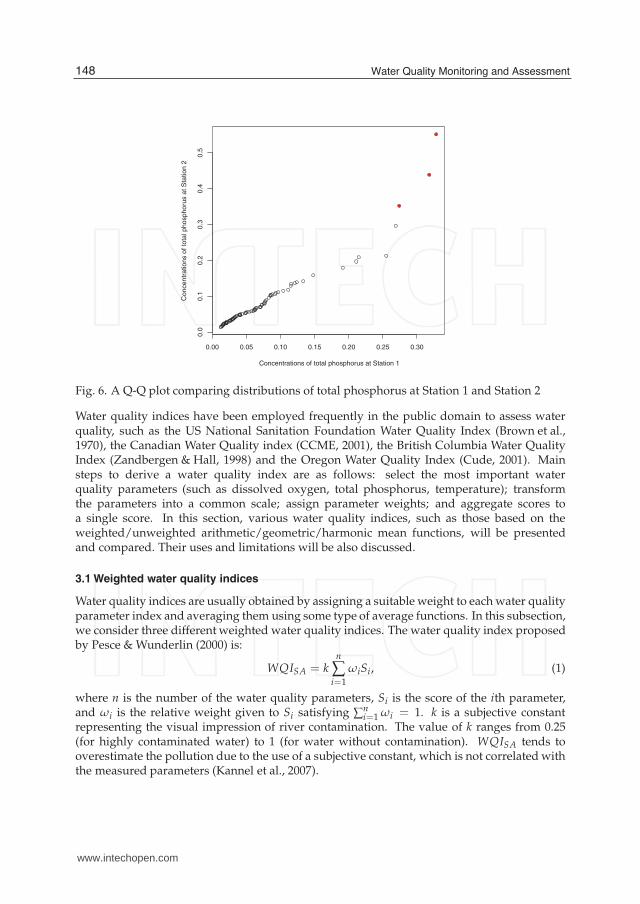
Fig. 5 (a) indicates that the distribution of total phosphorus concentrations is skewed to theright. Fig. 5 (b) shows an S-shape, but there is not sufficient evidence to prove that thedistribution of total phosphorus on the natural log scale is non-normal. Fig. 6 is a Q-Q plotcomparing whether two sample datasets are from populations with a common distribution.Note that there are also a few outliers appearing (possible outliers are in red). Otherwise, theplot suggests that the two samples have the same distribution.> qq <-qqplot(UNA$TP, CKL$TP, plot.it = TRUE, xlab = “Concentrations of total phosphorusat Station 1”, ylab =“Concentrations of total phosphorus at Station 2”)> points(qq$x[85],qq$y[85], pch=16, col=2)> points(qq$x[84],qq$y[84], pch=16, col=2)> points(qq$x[83],qq$y[83], pch=16, col=2)

3. Water quality index

Sometimes it is difficult to assess water quality from a large number of water qualityparameters. Traditional methods to evaluate water quality are based on the comparisonof experimentally determined parameter values with an existing local normative, whichdoes not provide a global summary on the spatial and temporal trends in the overall waterquality (Debels et al., 2005; Kannel et al., 2007). To integrate complex water quality data andprovide a simple and understandable tool for informing managers and decision-makers aboutthe overall water quality status, various water quality indices (WQI) have been developed,which can be used to give a global vision on the spatial and temporal changes of the waterquality. An early water quality index was proposed by Horton (1965), and then developedby Brown et al. (1970), Dojlido et al. (1994), McClelland (1974), and Pesce & Wunderlin (2000).


www.intechopen.com


0.00 0.05 0.10 0.15 0.20 0.25 0.30

0.0

0.1

0.2

0.3

0.4

0.5

Concentrations of total phosphorus at Station 1

Co

nce

ntr

atio

ns o

f to

tal p

ho

sp

ho

rus a

t S

tatio

n 2

Fig. 6. A Q-Q plot comparing distributions of total phosphorus at Station 1 and Station 2

Water quality indices have been employed frequently in the public domain to assess waterquality, such as the US National Sanitation Foundation Water Quality Index (Brown et al.,1970), the Canadian Water Quality index (CCME, 2001), the British Columbia Water QualityIndex (Zandbergen & Hall, 1998) and the Oregon Water Quality Index (Cude, 2001). Mainsteps to derive a water quality index are as follows: select the most important waterquality parameters (such as dissolved oxygen, total phosphorus, temperature); transformthe parameters into a common scale; assign parameter weights; and aggregate scores toa single score. In this section, various water quality indices, such as those based on theweighted/unweighted arithmetic/geometric/harmonic mean functions, will be presentedand compared. Their uses and limitations will be also discussed.

3.1 Weighted water quality indices

Water quality indices are usually obtained by assigning a suitable weight to each water qualityparameter index and averaging them using some type of average functions. In this subsection,we consider three different weighted water quality indices. The water quality index proposedby Pesce & Wunderlin (2000) is:

WQISA = kn

∑i=1

ωiSi, (1)

where n is the number of the water quality parameters, Si is the score of the ith parameter,and ωi is the relative weight given to Si satisfying ∑

ni=1 ωi = 1. k is a subjective constant

representing the visual impression of river contamination. The value of k ranges from 0.25(for highly contaminated water) to 1 (for water without contamination). WQISA tends tooverestimate the pollution due to the use of a subjective constant, which is not correlated withthe measured parameters (Kannel et al., 2007).


www.intechopen.com


Let k = 1 in Equation (1). In general, we have the objective water quality index originallyproposed by Horton (1965), hereafter called the weighted arithmetic water quality index. Ithas been used by many researchers (Brown et al., 1970; Prati et al., 1971; Sanchez et al., 2007):

WQIWA =n

∑i=1

ωiSi. (2)

The third water quality index is based on the weighted geometric mean function (Brown et al.,1970; McClelland, 1974), which is always smaller than WQIWA if all values of Si are positive:

WQIWG =n

∏i=1

Sωi

i . (3)

The above weighted water quality indices indicate that each water quality parameter mayhave different weights based on the importance of the water quality situation. Thischaracteristic could be desirable when water quality indices are specific to the protectionof aquatic life. However, when sensitivity to changes in each water quality parameteris more desirable than sensitivity to the most heavily weighted water quality parameter,such weighting could be unnecessary (Cude, 2001; Gupta et al., 2003; Landwehr & Deininger,1976). Some unweighted water quality indices were therefore explored (Cude, 2001;Dojlido et al., 1994; Landwehr & Deininger, 1976) and are now introduced in the followingsubsection.

3.2 Unweighted water quality indices

In this subsection, we introduce three unweighted water quality indices. The first two arearithmetic/geometric water quality indices proposed by Landwehr & Deininger (1976),

WQIA = 1/nn

∑i=1

Si, (4)

WQIG = (n

∏i=1

Si)1/n, (5)

which is a special case of (2) and (3) with ωi = 1/n for any i, respectively. As with therelationship between WQIWG and WQIWA, WQIG is always lower than WQIA. The third isthe harmonic square water quality index,

WQIH =

√

n

∑ni=1

1S2

i

, (6)

which has been suggested as an improvement over both WQIWA and WQIWG (Cude, 2001;Dojlido et al., 1994). Compared to WQIWA and WQIWG, WQIH is the most sensitive tochanges in single water quality parameter (Cude, 2001).

3.3 Harkins’ water quality index

An objective water quality index was proposed by Harkins (1974), which is based on Kendall’snonparametric multivariate ranking procedure.


www.intechopen.com


WQIHR =n

∑i=1

(Ri − Ric)2

var(Ri), (7)

where

var(Ri) =1

12M[(M3 − M)−

ki

∑j=1

(t3ij − tij)],

Ri and Ric correspond to the rank and control values of the ith water quality parameter,respectively. M is the number of water quality parameters plus the number of controlvalues, tij is the number of elements involved in the jth tie encountered when orderingthe measured values of the ith water quality parameter, and ki is the total number of tiesencountered in ranking the measurements of the ith parameter. Landwehr & Deininger(1976) and Gupta et al. (2003) compared WQIHR with water quality indices WQIWA, WQIWG,WQIG, and WQIA. Their results indicated that these five indices are correlated well with theopinions of experts, and although the five indices showed significant correlation with eachother, WQIHR was the lowest of the five. Therefore, they suggested adopting any of the fourindices except WQIHR.

4. Methods for handling data below detection limits

One feature of water quality measurement is that some data will fall above or below thedetection limit, and therefore not be captured, because of limitations of the measurementprocedures or the analytical tools used in the laboratories. Data below a detection limit arealso referred as left-censored data. There could also be multiple detection limits involvedif an instrument is upgraded during the project period or data are combined from multiplelaboratories. Even data below the detection limits are still of considerable importance becauseof the potential health hazard. The data below the detection limits complicate the analysis ofthe water quality data. Various strategies have been developed to analyze the data that fallbelow detection limits (Fu & Wang, 2011; Helsel, 1990; Shumway et al., 2002). In the followingsubsections, simple substitution methods, parametric methods, and nonparametric methodswill be introduced.

4.1 Simple deletion/substitution methods

Simple deletion/substitution methods delete/replace the measurements below detection

limits (DL) with fixed values, such as zero, 1/2DL, 1/√

2DL or DL (Helsel, 1990;Hornung & Reed, 1990). Hornung & Reed (1990) proposed using 1/

√2DL when the data

are not highly skewed and 1/2DL substitution otherwise. Hewett & Ganser (2007) found

that 1/2DL and 1/√

2DL perform well when the sample size is less than 20 and the percentcensored is less than 45 percent. It is easy and convenient to use the substitution methods.However, all tend to be biased and cause a loss of information (El-Shaarawi & Esterby, 1992;Helsel & Cohn, 1988; Lubin et al., 2004). When the results strongly depend on the values beingsubstituted, particularly for data with multiple detection limits (Shumway et al., 2002), thesubstitution methods are not generally suitable. In particular, when there is a high proportionof data below detection limits, results for standard errors are also far less desirable, and thebiased standard errors may further distort the inference (Helsel, 1990; 1992; Shumway et al.,2002).


www.intechopen.com


4.2 Parametric methods

Assume that the distribution of measurements is known, such as normal or lognormal.The data below the detection limits can be filled using values randomly selected from thedistribution or replaced with their conditional expected values (conditional on being lessthan the detection limits) (Helsel, 1990). Suppose that there are n detected measurements(y1, . . . , yn) and m measurements below the detection limits (c1, . . . , cm). The likelihoodfunction is

L(θ) =n

∏i=1

fθ(yi)m

∏j=1

Fθ(cj), (8)

where θ is a vector of parameter, f (·) is the probability density function of y, and F(·) is thecumulative density function (c.d.f.) of y. The parameter estimates of θ and summary statisticscan be obtained by the maximum likelihood method (ML) (Cohen, 1976; Cohn, 1988; Helsel,1992). Results based on a lognormal distribution assumption by the maximum likelihoodmethod can be easily obtained using statistic software R (NADA package) (Lee & Helsel,2005). If the distributional assumption is appropriate and the sample size is large, themaximum likelihood method is the most efficient (Cohn, 1988; Helsel, 1992; Hewett & Ganser,2007). To incorporate the covariate effects when analyzing the water quality data that fallbelow detection limits, the following regression models can be considered.

4.2.1 Tobit regression

Tobit regression model (Tobin, 1958) has been widely used to analyze censored data. Themodel can be written as

log(y∗i ) = β0 + β1xi + ǫi, (9)

where y∗ is a latent variable and yi = y∗i if y∗i > ci and yi = ci otherwise. Random error term

ǫi follows a normal distribution N(0, σ2). The likelihood function (8) can be written as

L(β0, β1) = ∏i

[

1

σφ

(

log(yi)− β0 − β1xi

σ

)]δi

∏i

[

Φ

(

log(ci)− β0 − β1xi

σ

)]1−δi

,

where δi = 1 if y∗i > ci and δi = 0 otherwise. The maximum likelihood estimates (MLE) ofparameters can be obtained from the function survreg (survival package) and vglm (VGAMpackage) in R if the detection limit is a single number. An example to obtain MLE ofparameters in a Tobit regression model log(DP) = β0 + β1log(Flow) + ǫ is given,> library(survival)> fit<- survreg(Surv(log(DP), DP>=0.01, type = ‘left’) ∼ log(Flow), data = UNA, dist =‘gaussian’)> summary(fit)For multiple detection limits, the estimates can be derived by a Newton-Raphson algorithm.The Wald type test or the likelihood ratio test can be applied to test the group differenceor covariate effects (by testing β = 0). Tobit regression is also applicable when both themeasurements of the response and covariate variable are with detection limits (Helsel, 1992).When the distribution is known and the error terms are homeostatic, the estimate derived bythe maximum likelihood method is optimal (Helsel, 2005b).


www.intechopen.com


4.2.2 Logistic regression

Let y = 1 if the response is above a detection limit c and y = 0 otherwise. Assume that theprobability of y = 1 is p, then p = p(y > c). A binary logistic regression modeled as a linearfunction of covariate x is given by

log(p

1 − p) = α0 + α1x.

The likelihood function is

L(α0, α1) = ∏i

pyi

i (1 − pi)1−yi ,

where pi = exp(α0 + α1xi)/[1 + exp(α0 + α1xi)]. The maximum likelihood estimates ofparameters can be obtained from glm function in R. The significance of the covariate effect canbe tested using the likelihood ratio statistic (Helsel, 1992). For multiple detection limits, theordered logistic regression can be used. More details can be seen in Helsel (1992). An exampleto obtain parameter estimates from a logistic regression log(p/(1 − p)) = α0 + α1log(Flow) isgiven as follows, where p = p(DP > 0.01).> UNA$ DPd<- 1-(UNA$ DPrem ==“<”)> logitfit<- glm(DPd ∼ log(Flow), data = UNA, family = binomial(“logit”))> summary(logitfit)

Parametric methods generally perform well for summary statistics when the dataset is largeand the underlying distribution can be approximated by a known distribution. Specificationof the underlying distribution of a dataset may be difficult in practical problems. The MLmethod does not work well when the distributional assumption is invalid or the sample sizeis small (<20) (Gleit, 1985; Helsel, 2005b; Helsel & Cohn, 1988). Furthermore, the ML methodis sensitive to outliers, which usually exist in water quality data. An implementation of fullyparametric methods is a robust and efficient semi-parametric regression method on orderstatistics (ROS) and will be introduced in the following subsection.

4.2.3 ROS method

The ROS method was provided by Helsel & Cohn (1988), which is a simple imputationmethod that fills in data below detection limits based on a probability plot of detections(Helsel & Cohn, 1988; Lee & Helsel, 2005; Shumway et al., 2002). It can be used to obtainsummary statistics, plot modeled distributions, and predict values based on the modeleddistributions (Fig. 7). The ROS method has been evaluated as one of the mostreliable approaches for estimating summary statistics of data with multiple detectionlimits (Shumway et al., 2002). Lee & Helsel (2005) developed software implementation thatperforms the ROS method, and it is a part of the NADA library in statistical software R. Rcodes for Fig. 7 are as follows:> library(NADA)> UNA<- UNA[!is.na(UNA$OP), ]> UNA$CenOP<- UNA$OPrem == “<”> rosop<- cenros(UNA$OP, UNA$CenOP, forwardT =“log”, reverseT = “exp”)> plot(rosop, plot.censored = TRUE)> lines(rosop, col = 2)


www.intechopen.com


−2 −1 0 1 2

Normal Quantiles

Va

lue

0.0

02

0.0

05

0.0

10

0.0

20

0.0

50

0.1

00

95

90

75

50

25

10

5

Percent Chance of Exceedance

Fig. 7. A normal Q-Q plot for a ROS model. Solid circles are detected data. Open circles aremodeled undetected values.

4.3 Nonparametric methods

Parametric and semi-parametric methods are based on the assumption of the underlyingdistribution of the data. Nonparametric methods provide an alternative that does not requirespecifying a distribution and filling in the data below detection limits. The nonparametricmethods are generally used to analyze the right censored data. Left censored data canbe converted into right-censored data by flipping the data over the largest observed value.Lee & Helsel (2007) provided software tools for direct analysis of data with multiple detectionlimits (left-censored data) by nonparametric modeling and hypothesis testing.

4.3.1 Kaplan-Meier

The Kaplan-Meier (K-M) method is the standard method for computing descriptive statisticsof data that fall below detection limits (Helsel, 2005; Lee & Helsel, 2007). K-M methodhas been widely used in survival analysis, where it is employed with right-censoredtime-to-failure data. The K-M method can estimate the percentiles or c.d.f. for a dataset,and can test hypotheses. It can describe and compare the shapes of different datasets (Figs. 8(a) and (b)).> KM<- cenfit(UNA$OP, UNA$CenOP)> plot(KM)> dat2<- dat2[!is.na(dat2$OP), ]> dat2$CenOP<- dat2$OPrem == “<”> g2<- cenfit(dat2$OP, dat2$CenOP,dat2$Station)> plot(g2,lty = c(1 : 3), col=c(1, 2, 4))> legend(0.002, 0.8, c(“Station 1”,“Station 2”,“Station 4”), lty = c(1:3), col=c(1, 2, 4))


www.intechopen.com


0.002 0.005 0.010 0.020 0.050 0.100

0.0

0.2

0.4

0.6

0.8

1.0

Value

Pro

babili

ty

(a) Dashed lines are 95% confidencelimits

0.002 0.005 0.010 0.020 0.050 0.100

0.0

0.2

0.4

0.6

0.8

1.0

Value

Pro

babili

ty

Station 1

Station 2

Station 4

(b) Empirical c.d.f at three stations

Fig. 8. Empirical cumulative distribution functions for datasets with multiple detection limits

Zhang et al. (2009) developed a nonparametric estimation procedure, and under a fixeddetection limit and some mild conditions, they established the theoretical equivalence of threenonparametric test statistics: the Wilcoxon rank sum, the Gehan, and the Peto-Peto tests.Their simulation studies indicated that nonparametric methods work well for a range of smallsizes and censoring rates (Zhang et al., 2009). For hypothesis testing with multiple detectionlimits, one robust method is to censor all data at the highest detection limit and then performan appropriate nonparametric test (Helsel, 1992). This can result in a loss of information,however, the accelerated failure time (AFT) model can integrate the Gehan and logrank tests,incorporate covariate effects, and compare the differences between two/multiple data groupswith multiple detection limits (Jin et al., 2006; Wei, 1992; Zhang et al., 2009).

4.3.2 AFT model

Assume that {Yi, i = 1, . . . , N}, {Ci, i = 1, . . . , N} and {Xi, i = 1, . . . , N} are measurements,detection limits and p × 1 covariate vector, respectively. Let Δi = 1 if Yi is below the detectionlimit Ci and Δi = 0 otherwise. Let Zi = min{− log(Yi),− log(Ci)}; therefore (Zi, Δi, Xi) arethe observations. The accelerated failure time model is

Zi = X′i β + ǫi,

where Zi = log(Yi), β is an unknown regression parameter vector, and ǫi is the errorterm. Suppose that {ǫi, i = 1, . . . , N} are independent and identically distributed and theirunderlying distribution is unknown.

Estimation and inference of the regression parameters are based on the estimating functionsgiven by

U(β) = N−2N

∑i=1

Δiω(ei)

{

Xi −∑

Nj=1 Xj I(ei ≥ ej)

∑Nj=1 I(ei ≥ ej)

}

,

where ω(ei) is a weight function and ei = log(Yi) − X′i βt, where βt is the true value of β.

Let ω(ei) = 1 and ω(ei) = ∑Nj=1 I(ei ≥ ej); U(β) correspond to the log-rank and Gehan


www.intechopen.com


statistics, respectively. The estimating functions U(β) are step functions and discontinuousin the regression parameters, which makes it difficult to find consistent estimators and theirasymptotic variance and covariance matrices. Much progress has been made to overcomethese difficulties (Brown & Wang, 2006; Heller, 2007; Jin et al., 2003; Lee et al., 1993), and thefunction lss (lss package) can be used to obtain various statistics from an AFT model.> library(lss)> UNA$status<- 1-(UNA$OPrem==“<”)> aftfit<- lss(cbind(log(OP), status)∼ log(Flow), data=UNA, gehanonly=FALSE, cov=TRUE)> print(aftfit)

Jin et al. (2006b) extended marginal accelerated failure time models to multivariate censoreddata. Their method, which is based on an independence “working" model, may ignorethe within-site correlations in obtaining parameter estimates, while taking account ofthe correlation in calculating the standard errors. More efficient estimators with similarcomputational complexity were developed for multivariate censored data analysis, whenmeasurements from the same site exhibit strong temporal correlations (Fu & Wang, 2011).

5. Trend detection

In recent years, concentrations of various water quality parameters have been collected.Tests for trends specific to various water quality parameters have been of keen interest inenvironmental science (Helsel, 1992). A number of methods have been proposed to detectand assess changes in water quality. In this section, a variety of approaches will be introducedand their strengths and weaknesses investigated. The exogenous variable effects and serialdependence will be considered when testing water quality trends.

5.1 Parametric methods

Under the normality of residuals and constant variance assumptions, simple/multiple linearregressions are preferable for detecting trends of water quality.

5.1.1 Simple linear regression

Let Y be the random variable of interest in a trend test, such as concentrations of water qualityparameters. T denotes time (often expressed in years). If Y is linear over time T, the linearsimple regression of Y on T is a test for trend.

Y = β0 + β1T + ǫ, (10)

where β1 is the rate of change in Y. The null hypothesis for testing the trend of y can be statedas a test for β1 = 0. The Wald type statistic (t-statistic) can be used. If the null hypothesisis rejected, it indicates that there is a linear trend in Y over time. If Y is not linear over timeT, some transformation of Y, such as a log transformation, may be necessary. An exampleusing a linear regression to detect the trend of total phosphorus concentrations at Station 1 ispresented in Fig. 9. The results indicate that the trend of total phosphorus is not significant.

5.1.2 Multiple regression

Most concentrations of water quality parameters have strong seasonal patterns (see Fig.10). They are influenced by the changes in biological activity, both natural and managed


www.intechopen.com


0.0

00

.05

0.1

00

.15

0.2

00

.25

0.3

0

Time

Co

nce

ntr

atio

ns o

f to

tal p

ho

sp

ho

rus (

mg

/L)

2006 2007 2008 2009 2010 2011

Fig. 9. Linear regression trend line for total phosphorus concentrationsRegression: C = 0.09 − 0.007Time, and p = 0.14

activities such as agriculture (Helsel, 1992; Hirsch et al., 1991). Therefore, it is importantto consider seasonal effects when evaluating changes in water quality data. In parametricprocedures, multiple regression with periodic functions can be used to describe seasonalvariation. Consider the following simple case,

Y = β0 + β1T + β2cos(2πT) + β3sin(2πT) + ǫ, (11)

where T is expressed in years and β1 indicates the change rate of Y. Terms sin(2πT) andcos(2πT) capture the annual cycle and account for seasonality. Residuals ǫ must follow anormal distribution (or approximately normal). The trend test can be constructed by testingβ1 = 0.

If residuals still show a seasonal pattern (see Fig. 11), additional periodic functions should beincluded in model (11) to remove the seasonal variation. A general multiple linear regressionis given by

Y = β0 + β1T +K

∑k=0

[β2k+1cos(2πkT) + β2k+2sin(2πkT)] + ǫ. (12)

The cases of K = 0 and K = 1 correspond to model (10) and (11). If K = 2, a period of 1/2 yearis then also included in model (12). Fig. 11 shows that the residuals of the linear regression inSubsection 5.1.1 represent a seasonal pattern, therefore periodic functions should be includedin the model.

When Y or some transformation of Y is linear with time T, and residuals follow a normaldistribution with a constant variance, the parametric regression is optimal. However, the


www.intechopen.com


2006 2007 2008 2009 2010 2011

0.0

00

.05

0.1

00

.15

0.2

00

.25

0.3

0

Time in years

Co

nce

ntr

atio

ns o

f to

tal p

ho

sp

ho

rus (

mg

/L)

Fig. 10. Time series plot of total phosphorus concentration at Station 1

−0

.05

0.0

00

.05

0.1

00

.15

0.2

00

.25

Time

Re

sid

ua

l

2006 2007 2008 2009 2010 2011

Fig. 11. Residuals of the linear regression mentioned in above subsection versus times in year.

distribution of water quality data is usually highly skewed, in particular, data related todischarge, as well as biological indicators (biomass, chlorophyll) (Helsel, 1992; Hirsch & Slack,


www.intechopen.com


1984). The test that depends on the normality assumption may be inappropriate. Thefollowing subsection introduces several nonparametric methods that do not require thenormality assumption.

5.2 Nonparametric methods

Water quality data usually have the following characteristics: nonnormal data, missing values,values below detection limits, and serial dependence. The nonparametric methods are robustand can handle these problems easily.

5.2.1 Mann-Kendall test

Mann (1945) and Kendall (1975) proposed a nonparametric test for randomness against trend.According to Mann (1945), the null hypothesis H0 states that (x1, . . . , xn) are a sample of nindependent and identically distributed random variables. The alternative hypothesis H1of atwo-sided test is that the distributions of xk and xj are not identical for all k, j ≤ n, and k �= j.The test statistic S is defined as

S =n−1

∑k=1

n

∑j=k+1

sgn(xj − xk),

where

sgn(θ) =

⎧

⎨

⎩

1 if θ > 00 if θ = 0−1 if θ < 0.

Under the null hypothesis, Mann (1945) and Kendall (1975) obtained the mean and varianceof S.

E(S) = 0,

var(S) = [n(n − 1)(2n − 5)− ∑t

t(t − 1)(2t − 5)]/18,

where t is the extent of any given tie (number of xs involved in a given tie) and ∑t denotes thesummation over all ties.

Both Mann (1945) and Kendall (1975) derived the exact distribution of S for n ≤ 10; provedthat the distribution of S is normal as n → ∞; and further showed that even for n = 10, thenormal approximate is excellent if one calculates the standard normal variate Z by

Z =

⎧

⎪

⎨

⎪

⎩

S−1{var(S)}1/2 if S > 0

0 if S = 0S+1

{var(S)}1/2 if S < 0.

Hence, in a two-sided test for trend, the H0 should be rejected if |Z| ≥ zα/2, where Φ(zα/2) =1− α/2, Φ(·) is the standard normal c.d.f. and α is the significance level for the test. A positionvalue of S indicates an “upward” trend, and a negative value of S presents a “downward”trend. For an example from Station 21 at Susquehanna River basin (Fig. 10), the statistic


www.intechopen.com


S = −90, the var(S) = 1096.67 under the null hypothesis and the p value is 0.0072, whichindicates a downward trend in the concentration of total phosphorus at Station 21.> library(Kendall)> TP<- ts(CONY$TP, frequency=1, start=1990)> mk<- MannKendall(TP)> summary(mk)

The seasonality is a common phenomenon, which indicates that the distributions differfor different times of year. The Mann-Kendall test therefore is sensitive to seasonality.Hirsch et al. (1982) developed a modified Mann-Kendall test to detect the trend of data withseasonality.

5.2.2 The seasonal Kendall test

Hirsch et al. (1982) presented a modified Mann-Kendall test that detects trends in time serieswith seasonal variation and called as a seasonal Kendall test. Let X = (X1, X2, · · · , Xm) andXi = (xi1, xi2, · · · , xini

), where X is the entire sample consisting of m subsamples Xi, and mis the number of seasons. Each subsample Xi contains ni annual values. The null hypothesisH0 is that X is a sample of independent random variables (xij), and that Xi is a subsample ofindependent and identically distributed random variables for i = 1, · · · , m. The alternativehypothesis H1 is that the subsample is not distributed identically. The test statistic proposedby Hirsch et al. (1982) is given as follows. For month i,

Si =ni−1

∑k=1

ni

∑j=k+1

sgn(xij − xik). (13)

Under the null hypothesis, Si is a Mann-Kendall test statistic and

E(Si) = 0,

var(Si) = [ni(ni − 1)(2ni − 5)− ∑ti

ti(ti − 1)(2ti − 5)]/18.

The distribution of Si is normal as ni → ∞ (ti is the extension of a given tie in month i). Definethe seasonal Kendall statistic

S∗ =m

∑i=1

Si, (14)

and its expectation

E(S∗) =m

∑i=1

E(Si) = 0,

and variance

var(S∗) =m

∑i=1

var(Si) +m

∑i=1

m

∑j �=i

cov(Si, Sj). (15)


www.intechopen.com


Under the null hypothesis, Si and Sj (j �= i) are independent, therefore

var(S∗) =m

∑i=1

[ni(ni − 1)(2ni − 5)− ∑ti

ti(ti − 1)(2ti − 5)]/18.

The standard normal variate Z∗ is defined as

Z∗ =

⎧

⎪

⎨

⎪

⎩

S∗−1{var(S∗)}1/2 if S∗

> 0

0 if S∗ = 0S∗+1

{var(S∗)}1/2 if S∗< 0.

The approximation is adequate for ni = 3 and m = 12 for all i (Hirsch et al., 1982). For theexample from Station 21 at Susquehanna River basin (Fig. 10), the statistic S∗ = −360, thevar(S) = 10779.67 under the null hypothesis, and the p value is 0.0005, which indicates adownward trend in the concentration of total phosphorus at Station 21.> library(Kendall)> TPS<- ts(c(t(RCON[,-1])), frequency = 12, start = c(1990, 1))> smk<- SeasonalMannKendall(TPS)> summary(smk)

A limitation of the seasonal Kendall test is one observation per month. If there are multipleobservations in each of the months, Hirsch et al. (1982) suggested using the medians ofthe multiple observations in the seasonal Kendall test. Another limitation is that theseasonal Kendall test is not robust against serial dependence. When serial dependence exists,cov(Si, Sj) in Equation (15) does not equal zero. Hirsch & Slack (1984) provided a modificationof the seasonal Kendall test which is robust against serial dependence, except when the datahave very strong long-term persistence or when the sample sizes are small. More details canbe found in Hirsch & Slack (1984) and Letternmatier (1988). In addition to detecting the trend,the magnitude of such a trend may also be desirable. In model (10), an estimate of β1 can beused to estimate the trend. For a seasonal Kendall test, calculate dijk = (Xij − Xik)/(j − k) forall pairs (Xik, Xij) and (k < j). Hirsch et al. (1982) proposed using the median of dijk as anestimator of the slope, which is robust against extreme values.

5.2.3 Sen’s T test

Farrel (1980) proposed an aligned-rank test for detecting trends, which is distribution freeand not affected by seasonal fluctuations (Van Belle & Hughes, 1984; Yu et al., 1993). Let xij

be the measurement in the ith month of the jth year at a sampling station, and i = 1, . . . m,j = 1, . . . , n. Let Rij be the rank of (xij − xi+) among the mn values of differences, wherexi+ = ∑

nj=1 xij. If ties occur, the average of the ranks is taken as the rank of each tie. The

statistic is

T =

{

12m2

n(n + 1) ∑i,j(Rij − Ri+)2

}1/2 { n

∑i=1

(i − n + 1

2)(R+j −

nm + 1

2)

}

,

where Ri+ = ∑j Rij/n and R+j = ∑i Rij/m. Under the null hypothesis of no trend, thedistribution of T tends to the standard normal distribution. Simulation results indicatedthat the normal approximation for the statistic T was reasonable even for a small sample(Van Belle & Hughes, 1984).


www.intechopen.com


The three nonparametric methods for detecting trends mentioned above have practically thesame power at a statistical significance level of 0.05 (Yu et al., 1993). It is worth noting thatthere may exist water quality parameters which exhibit strong evidence of a download trendin some months and then exhibit strong evidence of an upload trend (step trend) (Helsel, 1992;Hirsch et al., 1991). The methods described above all assume a single trend across all seasons,provide a summary statistic for the entire record (monotonic trend), and do not indicatewhen there are trends in opposing directions in different months. Van Belle & Hughes (1984)developed a statistic for testing homogeneity of trends. The statistic is

χ2homogeneous = χ2

total − χ2trend =

m

∑i=1

Z2i − mZ2,

where Zi = Si/√

var(Si), Si is the Mann-Kendall statistic in Equation (13), and Z =∑

mi=1 Zi/m. Under the null hypothesis that the seasons are homogeneous with respect to

trend, χ2homogeneous approximates the chi-square distribution with m − 1 degree of freedom.

If χ2homogeneous exceeds the critical value, it indicates that there are different trends among

different seasons. In that case, the three nonparametric methods are not meaningful, andthe Mann-Kendall statistic can be used to test the trend for each individual season.

5.3 Adjusting covariate effects on trend tests

Several variables (X) other than time trend usually have considerable influence on waterquality parameters (Y) (see Fig. 12). These variables are natural and random phenomena suchas rainfall, temperature, and stream flow. To detect the trend of water quality parameters withtime (T), these variable effects on water quality parameters need to be removed. The removalprocess includes modeling and explaining variable effects with regression methods and theLOWESS method (Helsel, 1992).> xyplot(log(TP)∼ log(Flow)|Year, col.line = 2, type=c("p", "r"), data = UNA, xlab = "Logvalues of flow", ylab = "Log values of total phosphorus concentrations")

5.3.1 Parametric methods

Consider a linear regression of Y versus time T and one or more covariates X,

Y = β0 + β1T + β2X + ǫ.

For the trend test, the null hypothesis is β1 = 0. The t-statistic can be used for the trend test.This model simultaneously explains the covariate effect and detects the trend with time. If thecovariate changes with time, the following regression can be considered.

Y = β0 + β1T + β2X + β3T ∗ X + ǫ,

where T ∗ X is the interactive term. For regression models, the relationship (linear function)between Y and X must be checked. Residuals should have no outliers and a constantcovariance. The functions in R for testing these assumptions can be found in Subsection 5.4.According to the previous analysis, we use the following multiple linear regression to detectthe trend of total phosphorus at Station 1. This model adjusts the flow effect and also capturesthe annual cycle.

ln(C) = 2.25 − 0.74Time − 0.43 sin(2πTime) + 0.22 cos(2πTime)

−1.81ln(Flow) + 0.096Time ∗ ln(Flow) + 0.15ln(Flow)2


www.intechopen.com


Log values of flow

Lo

g v

alu

es o

f to

tal p

ho

sp

ho

rus c

on

ce

ntr

atio

ns

−4

−3

−2

−1

5 6 7 8 9

2005 2006

5 6 7 8 9

2007

2008

5 6 7 8 9

2009

−4

−3

−2

−1

2010

Fig. 12. Log values of total phosphorus concentration (C) versus log values of flow (F)

The results indicate an annual cycle and flow effect exist (p<0.05). After adjusting exogenousvariables effects, the concentration of total phosphorus significantly decreases (p = 0.02).

5.3.2 Semi/nonparametric methods

Hirsch & Slack (1984) provided an adjusted seasonal Kendall test and proposed the followingmixture procedure to test trends: (a) Use a regression model Y = f (βX) + ǫ to find therelationship between the concentration and covariates, where f (·) is a certain function ofcovariate X; (b) If there exists a significant relationship, compute the adjusted concentrationYik − Yik, where Yik = f (βX) is the estimated concentration of Yik; (c) Then apply the seasonalKendall test for trend and slope estimator to the time series of Yik − Yik.

The nonparametric LOWESS method (Cleveland, 1979; Helsel, 1992) can be used to remove acovariate effect without previously assuming the form of the relationship between Y and X.It is solely determined by the dataset and therefore it is robust to the distribution of the datapattern. The function lowess in the statistical software R can be used to obtain the fitted valuesY of Y. The seasonal Kendall statistic (14) is calculated from Y − Y and T data pairs.

The parametric regression method can simultaneously check the covariate effect and detectthe trend. When the linearity and normality assumptions are met, the parametric regressionmethod outperforms for detecting and estimating the magnitude of trends. Otherwise, theLOWESS method is a desirable alternative. To examine the trend of a water quality parameter,the covariate and seasonal effects need to be removed. According to the real datasets, choosea reasonable statistical approach to test for trends. Various methods for trend tests are givenin Table 1. For water quality data with detection limits, parametric Tobit regression (9) can beused. When a fixed detection limit exists, all the data below the fixed detection limit can be


www.intechopen.com


considered to be tied with each other. The nonparametric procedures such as Mann-Kendall,and the seasonal Kendall statistics can be used directly. If multiple detection limits exist,censor the data at the highest detection limit and then use an appropriate method to test thetrend. Some information is certainly lost by making this change.

No exogenous covariate (X) effectsNo seasonality Seasonality

Parametric Regression of Y on T Regression of Y on T and Seasonal termsNonparametric M-K test S-K testMixed S-K test on residuals from regression of Y on X

Exogenous covariate (X) effects existNo seasonality Seasonality

Parametric Regression of Y on (T, X) Regression of Y on (T, X, S)Nonparametric M-K of residuals from regression of Y on (T, X) S-K of residuals from lowess of Y on XMixed M-K of residuals from regression of Y on (T, X) S-K of residuals from regression of Y on (T, X, S)

Table 1. Classification of various types of tests for monotonic trend. M-K indicatesMann-Kendall test, S-K indicates Seasonal Kendall test, and S denotes seasonal terms.

5.4 Computational implementation for linear regression models using R

In this subsection, we will show how to use the statistical software R to fit, evaluate andmodify a linear regression model. More details can be seen in Adler (2009), Crawley (2007),and Venables & Ripley (2002).

A linear regression model is one of the most classic and popular methods in statistical practice.It is a very important tool for the statistical analysis of water quality data. It assumes thatthere is a linear relationship between a response variable (continuous) and some covariatevariables. To fit a linear regression model to a dataset, the primary function is lm. We beginwith the dataset mentioned in Section 2 to show how to fit a linear model in R. R codes forfitting the dataset are as follows.> con.lm <- lm(log(TP) ∼ log(Flow) + pH, data = UNA)

To print a simple display of the fitted information, use the print function:> print(con.lm)

To obtain conventional regression analysis results, use the summary function:> summary(con.lm)

To extract the regression coefficients, use the coef or coefficients function:> coef(con.lm)

To obtain the variance-covariance matrix for the model fitted above, use the vcov or Varfunction:> vcov(con.lm)

To calculate the confidence intervals for the coefficients in the fitted model, use the confintfunction:>confint(con.lm, level = 0.95)

To get the residuals, use the resid or residuals function:> resid(con.lm)

To obtain the fitted values, use the fitted or fitted.values function:> fitted(con.lm)

To return the deviance of the fitted model, use the deviance function:> deviance(con.lm)

To refit the model, it is better to use the update function, which can save some typing. For


www.intechopen.com


example, a slightly different model is used to fit the data above, which considers an extracovariate “Temp” besides “Flow” and “pH”.> con.lm2<-update(con.lm, . ∼ . + Temp)

To compare models con.lm and con.lm2 which are used to fit the same dataset, use the anovafunction:> anova(con.lm, con.lm2)

The main arguments to the function lm are> lm(formula, data, weights, subset, na.action),

where formula is the model formula that specifies the form of the model to fit; data is anoptional data frame containing the variables in the model; weights is a positive numeric vectorcontaining weights to be used in the fitting process; subset is an optional vector specifyinga subset of observations to be used in the fitting process; and na.action is a function whichindicates how to handle missing values contained in the data.

The least-squares method performs well when the following key assumptions are satisfied: (1)There is a linear relationship between any pair of covariate variables (linearity); (2) The errorterms are normally distributed (normality) with a constant variance (homoscedasticity); (3)The error terms are not correlated with each other (autocorrelation). However, because theseassumptions may not be met in water quality data, linear regression is therefore not alwaysappropriate. The test functions can be used to check these assumptions in R. The functionncv.test in the car package can be used to test the homoscedasticity. The function durbin.watson(car package) is used to test autocorrelation in a linear regression model. Diagnostic plots canalso provide checks for homoscedasticity, normality, and influential observations (see Fig. 13),which can be obtained using the function plot(con.lm).

−4.0 −3.5 −3.0 −2.5 −2.0

−1

01

2

Fitted values

Resid

uals

Residuals vs Fitted

19

51

54

−2 −1 0 1 2

−2

−1

01

23


Sta

ndard

ized r

esid

uals

Normal Q−Q

19

51

54

−4.0 −3.5 −3.0 −2.5 −2.0

0.0

0.5

1.0

1.5

Fitted values

Sta

ndard

ized r

esid

uals

Scale−Location19

5154

0.00 0.02 0.04 0.06 0.08 0.10

−2

−1

01

23

Leverage

Sta

ndard

ized r

esid

uals

Cook’s distance

0.5

Residuals vs Leverage

51

40

38

Fig. 13. Diagnostic plots for a linear regression model


www.intechopen.com


6. Conclusions

Statistical methods are important in water quality analysis because much of what is knownabout water quality comes from numerical datasets. In this chapter, various statisticalmethods for analyzing water quality data have been introduced. Three typical graphs,boxplots, Q-Q plots, and scatter plots, which contain appropriate summarized informationabout datasets, are used to provide insight for analysts into datasets. A variety of classicwater quality indices are applied to give a global assessment of water quality. Weighted waterquality indices are relatively subjective; unweighted water quality indices and Harkins’ waterquality index are more objective. Other more advanced methods can be found in Raican et al.(2011) and Qian et al. (2007). To handle water quality data with detection limits, simplesubstitution methods as well as parametric and nonparametric approaches are investigated.Substitution methods are simple but possibly biased. Nonparametric methods which do notrequire the distributional assumption are robust and efficient (Helsel, 2005). Several popularmethods, such as Mann-Kendall, the seasonal Kendall test, and multiple regression methods,are provided to detect and assess changes of various water quality parameters (Helsel,1992). Meanwhile, nonlinear trends, serial dependence, covariate effects, and irregularmeasurement patterns need to be considered (Abaurrea et al., 2011; Morton & Henderson,2008). Computational implementation using R for linear regression models is introduced.Examples using a real dataset are given to illustrate some very useful R functions.

7. Acknowledgments

Dr. Liya Fu is a postdoc fellow whose research was supported by the Centre for Applicationsin Natural Resource Mathematics (CARM), School of Mathematics and Physics, the Universityof Queensland, Australia.

8. References

Abaurrea, J., Asín, J., Cebrián, C. C. & García-Vera, M. A. (2011). Trend analysis of waterquality series based on regression models with correlated errors, Journal of Hydrology,Vol. 400, 341–352.

Adler, J. (2009). R in a nutshell, O’Reilly Germany.Brown, R. M., McClelland, N. I., Deininger, R. A. & Tozer, R. G. (1970). A water quality index:

Do we dare? Water and Sewage Works, 117, 339–343.Brown, B. M. & Wang, Y-G. (2006). Induced smoothing for rank regression with censored

survival times, Statistics in Medicine, 26, 828–836.Canadian Council of Ministers of the Environment (CCME). (2001). Canadian water quality

guidelines for the protection of aquatic life, CCME water quality Index 1.0,Technical Report. In: Canadian environmental quality guidelines, 1999. Winnipeg:Canadian Council of Ministers of the Environment. http://www.ccme.ca/assets/pdf/wqi_techrprtfctsht_e.pdf.

Cleveland, W. S. (1979). Robust locally weighted regression and smoothing scatterplots,Journal of the American Statistical Association, 74, 829–836.

Cleveland, W. S., Grosse, E. & Shyu, W. M. (1992). Local regression models, Chapter 8 ofStatistical Models in S eds Chambers and Hastie, Wadsworth & Brooks/Cole.

Chambers, J. M., Cleveland, W. S., Kleiner, B. & Tukey, P. A. (1983). Graphical methods for dataanalysis, PWA-Kent Publishing Co., Boston.


www.intechopen.com


Cohen, A. C. (1976). Progressively censored sampling in the three parameter log-normaldistribution, Technometrics, Vol. 18, No. 1, 99–103.

Cohn, T. A. (1988). Adjusted maximum likelihood estimation of the moments of lognormalpopulations from type I censored samples, U.S. Geological Survey Open File Report,88–350,

Crawley, M. J. (2007). The R book, John Wiley & Sons Inc.Cude, C. G. (2001). Oregon water quality index: a tool for evaluating water quality

management effectiveness, Journal of the American Water Resources Association, 37,125–137.

Debels, P. and Figueroa, R. and Urrutia, R. and Barra, R. and Niell, X. (2005). Evaluation ofwater quality in the Chillán river (Central Chile) using physiochemical parametersand a modified water quality index, Environmental Monitoring and Assessment, Vol.110, No. 1301–322.

Dojlido, J. R., Raniszewski, J. & Woyciechowska, J. (1994). Water quality index applied to riversin the Vistula River Basion in Poland, Environmental Monitoring and Assessment, Vol.33, 33–42.

El-Shaarawi, A. H. & Esterby, S. R. (1992). Replacement of censored observations by a constant:an evaluation, Water Research, Vol. 26, Nol. 6, 835–844.

Farrel, R. (1980). Methods for classifying changes in environmental conditions, TechnicalReport VRF-EPA7. 4-FR80-1, Vector Research Inc., Ann Arbor, Michigan.

Fu, L. & Wang, Y-G. (2011). Nonparametric rank regression for analyzing water qualityconcentration data with multiple detection limits, Environmental Science andTechnology, Vol. 45, No. 4, 1481–1489.

Gleit, A. (1985). Estimation for small normal data sets with detection limits, EnvironmentalScience and Technology, 19, 1201–1206.

Gupta, A. K., Gupta, S. K. & Patil, R. S. (2003). A comparison of water quality indices forcoastal water, Journal of Environmental Science and Health, A38, 2711–2725.

Gnanadesikan, R. & Wilk, M. B. (1968). Probability plotting methods for the analysis of data,Biometrika, Vol. 55, 1–17.

Harkins, R. D. (1974). An objective water quality index, Journal of Water Pollution ControlFederation, Vol. 46, No. 3, 500–591.

Heller, G. (2007). Smoothed rank regression with censored data, Journal of the AmericanStatistical Association, Vol. 102, No. 478, 552–559.

Helsel, D. R. (1990). Less than obvious-statistical treatment data below the detection limit,Environmental Science and Technology, Vol. 24, No. 12, 1766–1744.

Helsel, D. R. (2005). Nondetects and data analysis: statistics for censored environmental data, Wiley:New York.

Helsel, D. R. (2005b). More than obvious: better methods for interpreting nondetect data,Environmental Science and Technology, 15, 419–423.

Helsel, D. R., Cohn, T. (1988) Estimation of descriptive statistics for multiply censored waterquality data, Water Resources Research, 24, 1997–2004.

Helsel, D. R. & Hirsch, R. M. (1992). Statistical methods in water resources, Elsevier Amsterdam,The Netherlands.

Hewett, P. & Ganser, G. H. (2007). A comparison of several methods for analyzing censoreddata, Applied Occupational and Environmental Hygiene, Vol. 51, No. 7, 611–632.


www.intechopen.com


Hirsch, R. M., Alexander, R. B. & Smith, R. A. (1991). Selection of methods for the detectionand estimation of trends in water quality, Water Resources Research, Vol. 27, No. 5,803–813.

Hirsch, R. M., Slack, J. R. & Smith, R. A. (1982). Techniques of trend analysis for monthly waterquality data, Water Resources Research, Vol. 18, 107–121.

Hirsch, R. M. & Slack, J. R. (1984). A nonparametric trend test for seasonal data with serialdependence, Water Resources Research, Vol. 20, No. 6, 727–732.

Hornung, R. W. & Reed, L. D. (1990). Estimation of average concentration in the presence ofnondetectable values, Applied Occupational and Environmental Hygiene, 5, 46–51.

Horton, R. K. (1965). An index-number system for rating water quality. Journal of WaterPollution Control Federation, Vol. 37, No. 3, 300–306.

Jin, Z., Lin, D. Y. & Wei, L. J. (2003). Rank-based inference for the accelerated failure timemodel, Biometrika, 90, 341–353.

Jin, Z., Lin, D. Y. & Ying, Z. (2006). On least-squares regression with censored data, Biometrika,93, 147–161.

Jin, Z., Lin, D. Y. & Ying, Z. (2006b). Rank regression analysis of multivariate failure time databased on marginal linear models, Scandinavian Journal of Statistics, 33, 1–23.

Kannel, P. R., Lee, S., Kanel, S. R. & Khan, S. P. (2007). Application of water quality indicesand dissolved oxygen as indicators for river water classification and urban impactassessment, Environmental Monitoring Assessment, Vol. 132, 93–110.

Kendall, M. G. (1975). Rank correlation methods, Charles Griffin, London.Landwehr, J. M. & Deininger, R. A. (1976). A comparison of several water quality indices,

Journal of Water Pollution Control Federation, Vol. 48, No. 5, 954–958.Lee, L. & Helsel, D. R. (2005). Statistical analysis of water-quality data containing multiple

detection limits: S-language software for regression on order statistics, Computer &Geosciences, 31, 1241–1248.

Lee, L. & Helsel, D. R. (2007). Statistical analysis of water-quality data containing multipledetection limits II: S-language software for nonparametric distribution modeling andhypothesis testing, Computer and Geosciences, 33, 696–704.

Lee, E. W., Wei, L. J. & Ying, Z. (1993). Linear regression analysis for highly stratified failuretime data, Journal of the American Statistical Association, 88, 557–565.

Lettenmaier, D. P. (1988). Multivariate nonparametric tests for trend in water quality, AmericanWater Resources Association, Vol. 24, No. 3, 505–512.

Lubin, J. H., Colt, J. S., Camann, D., Davis, S., Cerhan, J. R., Severson, R. K., Bernstein, L. &Hartge, P. (2004). Epidemiologic evaluation of measurement data in the presence ofdetection limits, Environmental Health Perspectives, 112, 1691–1696.

Mann, H. B. (1945). Non-parametric tests against trend, Econometrica, 13, 245–259.Alternative for handling detection limits data in impact assessments, Ground Water Monitor

Remediation, 4, 42–44.McClelland, N. I. (1974). Water quality index application in the Kansas river basin. U.S.

Environmental Protection Agency Region 7, Kansas City, Missouri.McGill, R., Tukey, J. W. & Larsen, W. A. (1978). Variations of box plots, The American Statistician,

Vol. 32, No.1, 12–16.Morton, R. & Henderson, B. L. (2008). Estimation of nonlinear trends in water quality: An

improved approach using generalized additive models, Water Resourse Research, Vol.44, W07420, doi:10.1029/2007WR006191.


www.intechopen.com


Prati, L., Pavenello, R. & Pesarin, F. (1971). Assessment of surface water quality by single indexof pollution, Water Research, 5, 741–751.

Pesce, S. F. & Wunderlin, D. A. (2000). Use of water quality indices to verify the impact ofCordoba city (Argentina) on Suquýa river, Water Research, 34, 2915–2926.

Qian, Y., Migliaccion, K. W., Wang, Y. S. & Li, Y. C. (2007). Surface water quality evaluationusing multivariate methods and a new water quality index in the Indian RiverLagoon, Florida. Water Recourses Research, 43, 1–10.

Raican, S. M., Wang, Y-G., Harch, B. (2011). Water quality assessments for reservoirs usingspatio-temporal data from balanced/unbalanced monitoring designs. submitted

Sanchez, E., Colmenarejo, M. F., Vicente, J., Rubio, A., Garcia, M. G., Travieso, L. & Borja,R. (2007). Use of the water quality index and dissolved oxygen deficit as simpleindicators of watersheds pollution, Ecological Indicators, 7, 315–328.

Shumway, R. H., Azari, R. S. & Kayhanian, M. (2002). Statistical approaches to estimatingmean water quality concentrations with detection limits, Environmental Science andTechnology, 36, 3345–3353.

Tobin, J. (1958). Estimation of relationships for limited dependent variables, Econometrica, Vol.26, No. 1, 24–36.

Tukey, J. W. (1977). Exploratory data analysis, Addison-Wesley Pub., Reading, MA.Van Belle, G. & Hughes, J. P. (1984). Nonparametric tests for trend in water quality, Water

Resources Research, Vol. 20, No. 1, 127–136.Venables, W. N. & Ripley, B. D. (2002). Modern applied statistics with S, Springer.Wei, L. J. (1992). The accelerated failure time model: a useful alternative to the Cox regression

model in survival analysis, Statistics in Medicine, Vol. 11, 1871–1879.Yu, Y.-S., Zou, S. & Whittemore, D. (1993). Non-parametric trend analysis of water quality

data of rivers in Kansas, Journal of Hydrology, Vol. 150, 61–80.Zhang, D. H., Fan, C. P., Zhang, J. & Zhang, C-H. (2009). Nonparametric methods for

measurements below detection limits, Statistics in Medicine, 28, 700–715.Zandbergen, P. A. & Hall, K. J. (1998). Analysis of the British Columbia water quality index for

watershed managers: a case study of two small watershelds. Water Quality ResearchJournal of Canada, 33, 519–549.


www.intechopen.com

Water Quality Monitoring and AssessmentEdited by Dr. Voudouris

ISBN 978-953-51-0486-5Hard cover, 602 pagesPublisher InTechPublished online 05, April, 2012Published in print edition April, 2012

InTech EuropeUniversity Campus STeP Ri Slavka Krautzeka 83/A 51000 Rijeka, Croatia Phone: +385 (51) 770 447 Fax: +385 (51) 686 166www.intechopen.com

InTech ChinaUnit 405, Office Block, Hotel Equatorial Shanghai No.65, Yan An Road (West), Shanghai, 200040, China

Phone: +86-21-62489820 Fax: +86-21-62489821

The book attempts to covers the main fields of water quality issues presenting case studies in variouscountries concerning the physicochemical characteristics of surface and groundwaters and possible pollutionsources as well as methods and tools for the evaluation of water quality status. This book is divided into twosections: Statistical Analysis of Water Quality Data;Water Quality Monitoring Studies.

How to referenceIn order to correctly reference this scholarly work, feel free to copy and paste the following:

Liya Fu and You-GanWang (2012). Statistical Tools for Analyzing Water Quality Data, Water QualityMonitoring and Assessment, Dr. Voudouris (Ed.), ISBN: 978-953-51-0486-5, InTech, Available from:http://www.intechopen.com/books/water-quality-monitoring-and-assessment/statistical-tools-for-analyzing-water-quality-data

statistical tools for analyzing water quality data · statistical tools for analyzing water quality...

Documents