statistical signal processing approaches to fault detection

www.elsevier.com/locate/arcontrol

Annual Reviews in Control 31 (2007) 41–54

Statistical signal processing approaches to fault detection§

F. Gustafsson

Department of Electrical Engineering, Linkopings Universitet, SE-581 83 Linkoping, Sweden

Received 27 September 2006; accepted 17 February 2007

Available online 7 May 2007

Abstract

The parity space approach to fault detection and isolation (FDI) has been developed during the last 20 years, and the focus here is to describe its

application to stochastic systems. A mixed model with both stochastic inputs and deterministic disturbances and faults is formulated over a sliding

window. Algorithms for detecting and isolating faults on-line and analyzing the probability for correct and incorrect decisions off-line are provided.

A major part of the paper is devoted to discussing properties of this model-based approach and generalizations to cases of incomplete model

knowledge, and non-linear non-Gaussian models. For this purpose, a simulation example is used throughout the paper for numerical illustrations,

and real-life applications for motivations. The final section discusses the reverse problem: fault detection approaches to statistical signal

processing. It is motivated by three applications that a simple CUSUM detector in feedback loop with an adaptive filter can mitigate the inherent

trade-off between estimation accuracy and tracking speed in linear filters.

# 2007 Elsevier Ltd. All rights reserved.

Keywords: Fault detection; Diagnosis; Kalman filtering; Adaptive filters; Linear systems; Principal component analysis; Subspace identification

1. Introduction

The parity space approach to fault detection (Basseville &

Nikiforov, 1993; Chow & Willsky, 1984; Ding, Guo, & Jeinsch,

1999; Gertler, 1997; Gertler, 1998) is an elegant and general

tool for additive faults in linear systems and is based on

intuitively simple algebraic projections and geometry. Simply

speaking, a residual rt is a data projection

rt ¼ PTZt; Zt ¼Yt

Ut

� �; (1)

where the data vector Zt contains the measured input (Ut) and

output (Yt) over a certain time window. The parity space

approach provides a tool to compute P that yields a residual

vector that is zero when there is no fault and non-zero otherwise.

A novel vector interpretation of the residual is presented,

with a direct link to vector quantization in communication

theory. Fault isolation is done by comparing the non-zero

residual to pre-computed fault vectors, and the closest one in a

statistical meaning is chosen in an on-line algorithm. The vector

approach provides an analytic approach to compute the

§ An earlier version of the paper was presented at SAFEPROCESS ’06,

Beijing, China, August 30–September 1, 2006.

E-mail address: [email protected].

1367-5788/$ – see front matter # 2007 Elsevier Ltd. All rights reserved.

doi:10.1016/j.arcontrol.2007.02.004

diagnosis probability matrix. This contains all probabilites of

giving an alarm of fault i given fault j has occured, where also

the non-faulty case is included (i; j ¼ 0). Faults that are hard or

even impossible to diagnose are discovered at this stage, and a

system or algorithm re-design can be performed.

This stochastic theory comes as a consequence of the model

assumptions. Section 4 motivates and generalizes the approach,

using a simulated DC motor example and several applications:

� A
n example of how a small measurement error can severely
perturb the standard parity space residual.

� A
motivating application for the Gaussian assumption for the
stochastic inputs.

� O
ne important alternative approach is the generalized
likelihood ratio (GLR) test, and it is pointed out that this

is actually equivalent to the stochastic parity space approach

for the model assumptions at hand.

� I
mplications of the length of the time window in theory and
for the example.

� E
xtensions and generalizations of the assumption of an
additive single fault of constant magnitude.

� A
successful application of the theory to a severely non-linear
systems, by linearizing around a nominal state trajectory.

� T
he relation to data-driven approaches as principal compo-
nent analysis (PCA).

mailto:[email protected]

http://dx.doi.org/10.1016/j.arcontrol.2007.02.004

F. Gustafsson / Annual Reviews in Control 31 (2007) 41–5442

� T
he use and fusion of residuals from several independent
models.

Fault detection preceeds fault isolation and involves making

a decision whether the residual rt is large enough, for instance if

its two-norm rTt rt exceeds a threshold. Some kind of post-

processing step of rTt rt is often needed in order to get a robust

fault detection algorithm. Here, the cumulative sum (CUSUM)

algorithm (Page, 1954; Basseville & Nikiforov, 1993;

Gustafsson, 2001) has proven very useful. The CUSUM test

recursively computes the decision statistic gt,

gt ¼ max

�gt�1 þ

rTt rt � EðrT

t rtÞVarðrT

t rtÞ� n; 0

�: (2)

Here, n is a drift, which acts similar to a forgetting factor in

adaptive filtering. The normalization of rTt rt above is conve-

nient for tuning purposes. The decision of a detected fault is

taken when gt exceeds a threshold, in which case the CUSUM

algorithm is restarted with gt ¼ 0.

The major part of the paper treats statistical signal

processing approaches to fault detection as outlined above.

However, classical statistical signal processing problems as

adaptive filtering can benefit from using fault detection ideas.

Section 5 gives three concrete application examples where fault

detection approaches to adaptive filtering are applied with very

good results.

The model and basic parity space relations are given in

Section 2. Section 3 provides the stochastic parity space theory,

and Section 4 the motivations and extensions. The reverse

problem of using fault detection for stochastic signal processing

is exemplified in Section 5, and Section 6 concludes the paper.

2. Parity space notation and models

The theory of parity space detection can be found in standard

references as Basseville and Nikiforov (1993), Chow and

Willsky (1984), Ding et al. (1999), Gertler (1997), and Gertler

(1998). The outline and notation below follows Chapter 11 in

(Gustafsson, 2001).

2.1. Model

The linear system is here defined as the state space model:

xtþ1 ¼ Atxt þ Bu;tut þ Bd;tdt þ B f ;t f t þ Bv;tvt (3a)

yt ¼ Ctxt þ Du;tut þ Dd;tdt þ D f ;t f t þ et: (3b)

The matrices At;Bt;Ct;Dt depend on the system, while the

signals belong to the following categories:

� D
eterministic known input ut, as is common in control
applications.

� D
eterministic unknown disturbance dt, as is also common in
control applications.

� D
eterministic unknown fault input f t, which is used in the
fault detection literature. We here assume that f t is either

zero (no fault) or proportional to the unit vector f t ¼ mtei,

where ei is all zero except for element i which is one. Exactly

which part of the system fault i affects is determined by the

corresponding columns in B f ;t and D f ;t. That is, we have

B f ;t f t ¼ Bif ;tmt, where Bi

f ;t is column i in B f ;t and similarly

for Dif ;t. This fault model covers offsets in actuators and

sensors for instance. The fault magnitude mt is assumed

constant magnitude mt ¼ m, but the time-varying fault case

will also be discussed.

� S
tochastic unknown state disturbance vt and measurement
noise et, as used in a Kalman filter setting. There is an

ambiguity of the interpretations of vt and dt. We might treat vt

as a deterministic disturbance, but in many cases this leads to

an infeasible problem where no parity space exists. Both vt

and et are here assumed to be independent with zero mean

and covariance matrices Qt and Rt, respectively.

� T
he initial state is treated as an unknown variable, so no prior
information is needed.

The dimension of any signal st is denoted as ns ¼ dimðstÞ.Traditionally, either a stochastic (dt ¼ 0) or a deterministic

(vt ¼ 0; et ¼ 0) framework is used in the literature, but here we

aim to mix them and combine the theories.

2.2. Parity space

There are many different derivations of the parity space. We

here use one based on the discrete time state space model in (3)

using data from a sliding window. In this case, the

measurements over a sliding window of size L can be

expressed explicitly in matrix form (without recursions) as

Yt ¼ Oxt�Lþ1 þ HuUt þ HdDt þ HvVt þ H f Ft þ Et: (4)

where Yt ¼ ðyTt�Lþ1 . . . yT

t ÞT

and

Hs ¼

Ds 0 . . . 0

CBs Ds . . . 0

..

.} ..

.

CAL�2Bs . . . CBs Ds

0BBB@

1CCCA; O ¼

CCA...

CAL�1

0BB@

1CCA:

(5)

Here H is defined for all signals s2fu; d; f ; vg. The covariance

matrix of the measurement vector is S ¼ CovðHvVt þ EtÞ.Without loss of generality, the residual generating matrix in

(1) can be defined as

rt ¼ WTðYt � HuUtÞ ¼ WTðI;�HuÞz}|{PT

Zt (6a)

rt ¼ WTðOxt�Lþ1 þ HdDt þ H f Ft þ HvVt þ Et|fflfflfflfflfflffl{zfflfflfflfflfflffl}S

Þ (6b)

The first equation is what can be computed on-line, and the

second expression is what will be used in the analysis.

The parity space is defined to be insensitive to the input

(yielding the factorization in (6a)), the initial state and

deterministic disturbances, which implies that rt ¼ 0 for any

initial state xt�Lþ1 and any disturbance sequence dk,

F. Gustafsson / Annual Reviews in Control 31 (2007) 41–54 43

k ¼ t � Lþ 1; . . . ; t, provided that there is no stochastic term

present (ek ¼ 0, vk ¼ 0). This is achieved if the projection

matrix satisfies the following condition.

� Parity space condition:

WTðOHdÞ ¼ 0,W 2N ½OHd �: (7)

Here, N A denotes the null space for the matrix A.

The projection matrix has dimension nr � Lny and is defined

to keep the sufficient information in the observations, while

information not useful for fault detection and isolation is

removed. A more abstract information based approach to split

up observations in different parts for the purpose of estimation

and fault detection is found in Levy, Benveniste, and

Nikoukhah (1996). The maximal dimension of the residual

vector is given by (see equation (11.12) in Gustafsson, 2001):

Lðny � ndÞ � nx � nr � Lny � nx (8)

The inequalities become an equality in case nd ¼ 0, that is,

no disturbance. Equality with the lower bound holds if the

matrix ðOHdÞ has full column rank. This shows that a parity

space always exists (nr > 0), if there are more observations than

disturbances and if L is chosen large enough.

3. Stochastic parity space theory

3.1. Residual distribution

From (6b) we get

EðrtÞ ¼ WTH f Ft; (9a)

CovðrtÞ ¼ WTSW : (9b)

For hypothesis testing and evaluation of detection prob-

abilities, we need the distribution for the residual conditioned

on that fault i has occurred. Assuming a constant fault

magnitude m for a while, the fault term f t ¼ mei in (3) can be

written H f Ft ¼ Hif 1Lm in (6). This notation will be used in the

sequel.

Further, if the residual distribution is assumed Gaussian,

then

ðrtjm f iÞ 2Nðm WTHif 1|fflfflfflffl{zfflfflfflffl}

mi

;WTSWÞ: (10)

The Gaussian distribution can be motivated in two ways:

� I
t is Gaussian if both Vt and Et are Gaussian.
� I
t is approximately Gaussian by the central limit theorem
when dim rt� dim Vt þ dim Et, which happens if the data

window L is large enough. That is, asymptotically in L, it is

Gaussian.

The parity space is unique up to a multiplication with a

unitary matrix, so the projection matrix can be pre-multiplied

with any full rank matrix. One solution is to take any

WT 2N ½OHd �, but the main alternatives are the following ones:

� S
tructured residual:
WT ¼ N ½OHd � : WTHif 1 ¼ ei; (11)

� N
ormalized residual:
WT ¼ N ½OHd � : WTSW ¼ I: (12)

Structured residuals are the suggested approach in many

publications, as Keller (1999), and White and Speyer (1987).

The normalized residual can be derived from any parity space

in the following way:

� N
ormalized parity space:
rt ¼ WTðYt � HuUtÞ; W

T ¼ ðWTSWÞ�1=2WT; (13)

for any parity space WT, where S ¼ CovðEt þ HvVtÞ.

We call kWTHi

f 1Lk ¼ kðWTSWÞ�1=2WTHi

f 1Lk the fault to

noise ratio (FNR).

3.2. Illustrative example

As an illustrative example throughout the paper, we consider

a DC motor subject to faults in input voltage (equivalent to a

torque disturbance) or a velocity sensor offset:

xtþ1 ¼1 0:3297

0 0:6703

� �xt þ

0:0703

0:3297

� �ut þ

0:08

0:16

� �vt

þ 0:0703 0

0:3297 0

� �f t;

yt ¼1 0

0 1

� �xt þ

0 0

0 1

� �f t þ et; Q ¼ 0:012;

R ¼ 0:12I:

With L ¼ 2, the parity space residual becomes two-

dimensional and easy to visualize graphically. There are also

two possible faults to isolate. Fig. 1 illustrates the distribution

of the structured and normalized parity space residual,

respectively, for the cases of no fault and fault, respectively.

For the special case of known fault magnitude m, the

decision boundary for the structured residual becomes a non-

linear curve, while diagnosis for normalized residuals is based

on the straight decision lines dashed in Fig. 1(b). For the general

case of unknown m, fault isolation is based on which fault

vector has the smallest angle to the observed stochastic

residual.

3.3. On-line algorithm

For normalized residuals ðrtj f ¼ 0Þ 2Nð0; IÞ, we have

ðrTt rtj f ¼ 0Þ 2x2ðnrÞ. The x2 test provides a threshold h for

detection, and fault isolation is performed by taking the closest

Fig.1. Structured andnormalized residual faultpatternwith uncertaintyellipsoids

for faults 1 and 2, respectively. (a) Structured residual; (b) normalized residual.


fault vector in the sense of smallest angle difference (since the

magnitude m of m is unknown in general).

Algorithm 1 (On-line diagnosis).

1. C
ompute a normalized parity space W, e.g. (13).
2. C
ompute recursively:
� Residual:

rt ¼ WTðYt � HUUtÞ

� Detection:

rTt rt > h

� Isolation:

i ¼ arg mini

�� rt

krtk� mi

kmik

��2

¼ arg mini

angleðrt; miÞ

where rTt rt 2x2ðnrÞ and angleðrt; m

iÞ denotes the angle

between the two vectors rt and mi. A detection may be

rejected if no suitable isolation is found (min iangleðrt; miÞ

is too large) to improve false alarm rate.

For diagnosability of single faults, the only requirement is

that all faults are mapped to different directions mi. Thus, in

theory infinitely many faults can be isolated even from a two-

dimensional residual.

In case of multiple faults, the fault vector is a linear

combination m ¼Pn f

i¼1 aimi and the isolation step in Algorithm

1 does not apply as stated. In such case, a least squares estimate

of the linear coefficients can be done, and the isolation step can

be modified accordingly. Normally, only one or a few faults

occur at the same time, so most coefficients ai should be

constrained to zero.

In a two-dimensional normalized residual space, as in the

example in Fig. 1(b), the probability for false alarm, PFA

(incorrect detection) can be computed explicitly as

PFA ¼Z

rTt rt > h

1

2pe�rT

t rt=2 drt ¼Z 2p

0

Z 1h

x

2pe�x2=2 dx df

¼ e�h2=2:

This means that the detection circle in Fig. 1(b) has a radius

h that can be directly computed from the desired false alarm

rate. A more precise analysis is given below.

3.4. Off-line analysis

We can interpret the fault isolation step as a classification

problem, and compare it to modulation in digital communica-

tion. Performance depends on the SNR, which here corresponds

to FNR mkmik. In vector coding in communication theory,

using an additive Gaussian error assumption, it is straightfor-

ward to compute the risk for incorrect symbol detection. We

will here extend these expressions from regular 2D (complex

plane) patterns to general vectors in Rnr .

The risk of incorrect diagnosis can be computed exactly in

the case of only two faults as follows. It relies on the symmetric

distribution of rt, where the decision region becomes a line, as

illustrated by the dashed lines in Fig. 1(b). The first step is a

change of coordinates to one where one axis is perpendicular to

the decision plane. Because of the normalization, the Jacobian

of this transformation equals one. The second step is to

marginalize all dimensions except the one perpendicular to the

decision plane. All these marginals integrate to one. The third

step is to evaluate the Gaussian error function. Here we use the

definition

erfcðxÞ ¼Z 1

x

1ffiffiffiffiffiffi2pp e�x2=2dx

The result in R2 (cf. Fig. 1) can be written

Pðdiagnosis ijfault m f jÞ ¼ erfc

�mkm jksin

�ai � a j

2

��:

(14)

In the general case, the decision line becomes a plane, and

the line perpendicular to it is given by the projection distance to

the intermediate line m1 þ m2 as

m

�m1 � m1; m1 þ m2

m1 þ m2; m1 þ m2ðm1 þ m2Þ

�; (15)

where ða; bÞ ¼ aTb denotes a scalar product, and we get the

following algorithm:


Algorithm 2 (Off-line diagnosis analysis).

1. C
ompute a normalized parity space W , e.g. (13).
2. C
ompute the normalized fault vectors mi in the parity space.
3. T

Fig. 2. Parity space residual for a DC motor for the residual distribution in

Fig. 1. The motor is subject to first an input voltage offset and then a sensor

offset. The two residuals are designed to be non-zero for only one fault each.

The lower plot illustrates extremely high sensitivity in residuals to measurement

noise (SNR ¼ 221).

he probability of incorrect diagnosis is approximately

Pðdiagnosis ijfault m f jÞ

¼ erfc

�m

��m j � m j; m j þ mi

m j þ mi; m j þ miðm j þ miÞ

��

(16)

Here m denotes the magnitude of the fault. If this is not

constant, replace mi ¼ WTHi

f 1Lm with mi ¼ WTHi

f Mt.

For more than two faults, this expression is an approxima-

tion but, just as in the case of vector coding, generally quite a

good one. The approximation becomes worse when there are

several conflicting faults, which means that there are three or

more fault vectors in about the same direction.

We can now define the diagnosability matrix P as

Pði; jÞ ¼ Pðdiagnosis ijfault f jÞ; i 6¼ j;

Pð j; jÞ ¼ 1�Xi 6¼ j

Pði; jÞ:(17)

It tells us everything about fault association probabilities for

normalized faults m ¼ 1, and the off-diagonal elements are

monotonically decreasing functions of the fault magnitude m.

Furthermore, in the classification we should allow the non-

faulty class (0), where f ¼ 0, to decrease the false alarm rate by

neglecting residual vectors, though having large amplitude,

being far from the known fault vectors. Consider for instance

the residual rt ¼ ð�1;�1ÞT in Fig. 1(b). This would most likely

be caused by noise, not a fault. The missed detection

probabilities are computed in a similar way as

Pðdiagnosis 0jfault f jÞ ¼ 1

2erfc

�mkm jk

2

�(18a)

Pð0;0Þ ¼ 1�X

j

Pð0; jÞ<PFA: (18b)

For the DC motor residuals with residuals distributed

according to Fig. 1, the diagnosis probability matrix is

Pð1:2;1;2Þ ¼ 0:995 0:005

0:005 0:995

� �: (19)

4. Stochastic parity space FAQ

We now have the basic tools for fault detection and isolation,

and it remains to conclude if this approach is useful in practice.

There are many natural questions, and the following subsec-

tions contain partial answers to some of them.

4.1. Why bother about noise?

If the fault is large enough, any diagnosis approach will

work. The critical case is when the fault to noise ratio is rather

small. Fig. 2 shows how a two-dimensional parity space

residual reacts to the two simulated faults in the DC motor.

The upper plot in 2 shows the case with no measurement

noise eiðtÞ ¼ 0. The transient in the residual filter can be

avoided with a slightly different design, otherwise the residual

response is perfect, and the correct diagnosis can be made.

The lower plot in Fig. 2, however, reveals that the design is

rather sensitive to noise. Diagnosis based on these residuals

becomes more or less random. There are two approaches to

robustify FDI:

� P
re-filter the system inputs and outputs, or post-filter the
residuals. The post-filter can be a linear low-pass filter, non-

linear threshold counter or the CUSUM test (2).

� M
ake a stochastic analysis of the problem and an appropriate
design.

The former approach is probably the dominating one in

practice. The second approach is the soundest one if the model

assumptions are plausible. More on these assumption follows

below.

4.2. Does Gaussian noise exist in practice?

An often heard criticism to stochastic approaches to control

and signal processing is that Gaussian noise is a theorectical

concept which is seldom useful in practice. While there certainly

are many diagnosis problems where a Gaussian model is notplau-

sible, there are others where this a very well-founded assumption.

Here, we illustrate the Gaussian assumptions with measure-

ments from the IMU in Fig. 3 as presented in Tornqvist (2006).

The sensor and application are described in Chandaria et al.

(2006).

Fig. 4 shows the histogram of the nine available measure-

ments from this unit. Clearly, the Gaussian bell fits well to the

Fig. 3. Miniature inertial measurement unit (IMU) by xsens.com with 3D

measurements of acceleration, angular speeds and magnetic field as well as a

built in camera.


observations. The correlation function plots presented in

Tornqvist (2006) confirm independence in time. However, as

shown in Fig. 5, the measurements from the magnetometer is

not spatially white, so the covariance matrix is full. This is also

true for accelerometers and gyroscope measurements.

4.3. Which are the design parameters?

The principal design parameter is the size L of the sliding

window. When L is increased, more information is used in the

diagnosis and a better result is expected. Fig. 6 illustrates how the

confidence circles of the residuals become more separated when

L is increased. A larger L means that it takes a longer time to get a

complete window with faulty data, so the delay for detection

should increase with L. This is the basic performance trade-off.

Fig. 4. Histograms of measurement

Fig. 7 shows a systematic evaluation of the design parameter

L. The miss-classification probabilities decrease quickly in L.

For the DC motor, we have lim L!1P ¼ I.

The diagnosis probability matrix can also be used for sensor

choice and system design in general.

4.4. Why not using the GLR test?

Once the distribution of the stochastic inputs is known,

Gaussian or not, the generalized likelihood ratio (GLR) test is

the natural approach, since it has many appealing properties.

For instance, it is the uniformly most powerful (UMP) test

under certain conditions (Kay, 1998). The GLR test statistic for

fault i for data in the sliding window considered here is given

by

git ¼

max x;m pðYtjxt�Lþ1;m; fault iÞmax x pðYtjxt�Lþ1; no faultÞ (20)

for fault i.

However, it is shown in Tornqvist and Gustafsson (2006)

that the GLR test and stochastic parity space tests are

equivalent. That is, which approach is used does not matter

in the end, since they both lead to the same algorithms.

4.5. How many faults can be detected?

In the case that one or more faults may be present, a

necessary condition for diagnosability is nr � n f . That is,

there must be at least as many residuals as faults. A sufficient

condition is that WT½H1f 1; . . . ;H

n f

f 1� has full column

rank.

errors from the IMU in Fig. 3.

Fig. 5. Scatter plot of magnetometer measurements when the IMU is lying on a table. The projections using equal axis scaling indicates spatial correlation.


For single faults, these conditions can be relaxed. Similar to

vector coding techniques, there can be arbitrarily many faults

that are diagnosable if nr � 2. To illustrate this, a more complex

system is used (F16 pitch dynamics with five states, three

Fig. 6. Similar to Fig. 1, but with L increased from 2 to 3. The circles are now

more separated, decreasing the risk of incorrect decisions.

inputs, three outputs and six faults) (see Hagenblad,

Gustafsson, & Klein, 2003 for details). Fig. 8 illustrates a

four dimensional residual (L ¼ 2).

The residual indicates that fault four is not detectable, and

faults 2 and 5 are hard to distinguish. This is also revealed in the

diagnosis probability matrix from Algorithm 2:

P ¼

1:0000 0:0000 0:0000 0 0:0000 0:0000

0:0000 0:5980 0:0000 0 0:4020 0:0001

0:0000 0:0000 0:9999 0 0:0001 0:0000

0 0 0 0 0 0

0:0000 0:4020 0:0001 0 0:5415 0:0564

0:0000 0:0001 0:0000 0 0:0564 0:9436

0BBBBBB@

1CCCCCCA:

(21)

Fig. 7. Miss-classification probabilities in diagnosis as a function of sliding

window length, where (19) gives the full matrix for L ¼ 2.

Fig. 8. Illustration of the residuals from parity space for no fault (0) and faults

1–6, respectively, but here in another basis. The decision lines for fault isolation

for known m are indicated.

Fig. 9. Sum of squared residuals rTt rt in case of no fault.


4.6. What happens if the fault magnitude is time-varying

In the analysis, it was assumed that the fault is m f i, where m

is the magnitude and f i the direction of the fault. The original

model (6) allows for general fault profiles in the fault term

H f Ft. However, letting Ft be arbitrary gives too much freedom

and any noise influence can be interpreted as a fault, since H f

generally spans the whole measurement space for Yt. A natural

model-based approach to model an incipient fault that grows

gradually in time or fluctuates slowly is to use a dedicated

model for the fault magnitude mt. For instance, a low order

polynomial model is used in Hendeby and Gustafsson (2006),

and Tornqvist (2006). This will reduce the span of H f to a low

dimensional space, where noise and fault can be better

separated.

4.7. What happens if the model is non-linear?

Possible approaches for non-linear stochastic systems

include:

� L
inearize the model in the same spirit as the extended
Kalman filter (KF). Here, the linearized model is used over a

time horizon of size L, which puts a further requirement on

this design variable. It cannot be chosen arbitrarily large,

since in that case the linearized model becomes poorer. One

should note that the linearization can pose a fault masking

effect making certain faults invisible.

� U
se non-linear filters as the particle filter (PF) (see Azimi-
Sadjadi & Krishnaprasad, 2002; Kadirkamanathan, Li,

Jaward, & Fabri, 2002; Vaswani, 2004; Hendeby &

Gustafsson, 2006).

The first approach is suitable for the stochastic parity space

approach. The IMU in Section 4.2 is here re-visited. The

intended task is to estimate orientation based on the IMU in

Fig. 3. This is done by dead-reckoning gyroscope measure-

ments. To avoid drift in time, supporting information with

respect to the earth frame is needed. The magnetometer gives

two degrees of freedom, and when the IMU is still, the

accelerometer vector can be used as an inclinometer, once the

gravity field is subtracted. This is state of the art, as described in

for instance Roetenberg, Luinge, Baten, and Veltink (2005).

The orientation dynamics as used in Tornqvist (2006) is

based on quaternions as state vector xt. The process model

xtþ1 ¼ f ðxt; ut; vtÞ is quite non-linear, and so are the

measurement equations yt ¼ hðxt; etÞ. The dynamics is quite

fast, so a fixed linearization state cannot be used. The

orientation may change too much during the sliding window.

Instead, the model is linearized around the nominal trajectory in

the sliding window, which is obtained by integrating the

gyroscope signals (here considered as inputs ut). This leads to

an error state model, with much slower dynamics. The size of

the residual computed from the accelerometers and magnet-

ometers, respectively, is 26 (L ¼ 10, ny ¼ 3, nx ¼ 4, nd ¼ 0 in

(8)), so the test statistic should be distributed as x2ð26Þ in

theory.

Fig. 9 shows how the two test statistics vary in time. There is

a perfect match between theory and experiment, which

validates the involved assumptions:

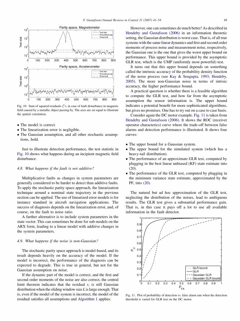
Fig. 10. Sum of squared residuals rTt rt in case of fault disturbance in magnetic

field caused by a metallic object passing by. The axes are set equal to illustrate

the spatial correlation.


� T
he model is correct.
� T
he linearization error is negligible.
� T

Fig. 11. Plot of probability of detection vs. false alarm rate when the detection

threshold is varied for GLR test on the DC motor.

he Gaussian assumption, and all other stochastic assump-

tions, hold.

Just to illustrate detection performance, the test statistic in

Fig. 10 shows what happens during an incipient magnetic field

disturbance.

4.8. What happens if the fault is not additive?

Multiplicative faults as changes in system parameters are

generally considered to be harder to detect than additive faults.

To apply the stochastic parity space approach, the linearization

technique around a nominal state trajectory in the previous

section can be applied. The use of linearized error models is for

instance standard in aircraft navigation applications. The

success of diagnosis depends on the linearization error, and, of

course, on the fault to noise ratio.

A further alternative is to include system parameters in the

state vector. This can sometimes be done for sub-models on the

ARX form, leading to a linear model with additive changes in

the system parameters.

4.9. What happens if the noise is non-Gaussian?

The stochastic parity space approach is model-based, and its

result depends heavily on the accuracy of the model. If the

model is incorrect, the performance of the diagnosis can be

expected to degrade. This is true in general, but not for the

Gaussian assumption on noise.

If the dynamic part of the model is correct, and the first and

second order moments of the noise are also correct, the central

limit theorem indicates that the residual rt is still Gaussian

distribution when the sliding window size L is large enough. That

is, even if the model of the system is incorrect, the model of the

residual satisfies all assumptions and Algorithm 1 applies.

However, one can sometimes do much better! As described in

Hendeby and Gustafsson (2006) in an information theoretic

setting, the Gaussian distribution is worst case. That is, of all true

systems with the same linear dynamics and first and second order

moments of process noise and measurement noise, respectively,

the Gaussian one is the one that gives the worst upper bound on

performance. This upper bound is provided by the asymptotic

GLR test, which is the UMP (uniformly most powerful) test.

It turns out that this upper bound depends on something

called the intrinsic accuracy of the probability density function

of the noise process (see Kay & Sengupta, 1993; Hendeby,

2005). The more non-Gaussian noise in terms of intrisic

accuracy, the higher performance bound.

A practical question is whether there is a feasible algorithm

to compute the GLR test, and how far from the asymptotic

assumption the sensor information is. The upper bound

indicates a potential benefit for more sophisticated algorithms,

but gives no promises. One has to try out on a case to case basis.

Consider again the DC motor example. Fig. 11 is taken from

Hendeby and Gustafsson (2006). It shows the ROC (receiver

operator characterics) curve where the trade-off between false

alarms and detection performance is illustrated. It shows four

curves:

� T
he upper bound for a Gaussian system.
� T
he upper bound for the simulated system (which has a
heavy-tail distribution).

� T
he performance of an approximate GLR test, computed by
plugging in the best linear unbiased (KF) state estimate into

(20).

� T
he performance of the GLR test, computed by plugging in
the minimum variance state estimate, approximated by the

PF, into (20).

The natural but ad hoc approximation of the GLR test,

neglecting the distribution of the noises, lead to ambiguous

results. The GLR test gives a substantial performance gain.

That is, in this case it pays off a lot to use all available

information in the fault detector.


4.10. What happens if there is no model available?

Approaches to compute the projection P in (1) include the

following options, starting with the one based on a physical

model and ending with a completely data-driven approach:

(1) T
he model-based parity space, where PðA;B;C;DÞdepends on the known state space model, described by
the quadruple ðA;B;C;DÞ.
(2) S ystem identification gives ðA; B; C; DÞ, from which the
parity space can be approximated as PðA; B; C; DÞ. One

here needs to know the structure of the state space model.

(3) C

Fig. 12. Comparison of residuals from parity space on known model, parity

ertain subspace approaches to system identification, as the

one in Verhaegen (1994), provide a way to directly compute

P (Zhang & Ding, 2005). Again, one needs to know the

structure of the state space model.

space using estimated model, and PCA residuals. The identified model and PCA
(4) T
analysis were performed on the same data set, thus using the same information.

he principal component analysis (PCA) approach (Dunia,

Qin, Edgar, & McAvoy, 1996; Qin & Li, 1999), where one

directly estimates P from data. Compared to above, one needs

to know the state order, but not how the data Zt is split into

inputs and outputs. That is, causality is no concern in the PCA

approach. This is one main reason for its wide spread in

chemical engineering, where sometimes thousands of

variablesare measured (see Chiang, Russell,& Braatz, 2001).

All cases can be unified in the following algorithm:

(1) D
etermine the projection matrix P as outlined above.
(2) E
stimate the residual covariance matrix from training data
from a fault-free system, and normalize the residuals:

S ¼ 1

N � L

XN

t¼Lþ1

rtrTt (22a)

rt ¼ S�1=2

rt: (22b)

(3) G
et learning data from each faulty mode and compute the
normalized fault vector as

mi ¼1

Ni � L

XNi

t¼Lþ1

rit: (23)

Fig. 12 shows how the probability of detection for each fault

in the DC motor example depends on the fault magnitude using

Monte Carlo simulations. The same data sets are used for all

three approaches.

The difference in performance is not very significant, despite

the large difference in prior information. In an attempt to

understand the relation between PCA and parity space, consider

the following split of our model:

Zt ¼O0

� �xt�Lþ1 þ

H f ; Hu; Hv; I0; I; 0; 0

� � FUVE

0BB@

1CCA

¼ Pxxt�Lþ1 þ Prrt: (24)

PCA splits the covariance matrix of data Zt based on its

eigenvalues into two parts: the model and the residuals. This

results in an expression of the same form as (24). We conclude

the following relations:

� T
he split of eigenvalues should give rankðPxÞ ¼ nx.
� T
he inputs in the data are revealed by zero rows in Px, so
causality is cleared out.

� T
he residual part must also explain dynamics in the input
data, and changes in input dynamics can be mixed up with

system changes.

� I
t cannot be guaranteed that the eigenvalues of the system are
larger than the other ones, so the PCA split based on sorted

eigenvalues can be dubious.

Despite the two last points, the example demonstrates

excellent performance, though these points should be kept in

mind.

4.11. What happens if there are many models?

In some applications, there might be many models that relate

to the fault. One example is road-friction estimation in Section

5.1 where a change in friction can be detected from sound,

visual information, longitudinal and lateral dynamic behaviour

of the vehicle, tire vibrations, or even from the driver behaviour

(see Muller, Uchanski, & Hedrick, 2003; Gustafsson, 1997).

Another currently hot topic in automotive safety is tire

pressure monitoring systems (TPMS), which is proposed to be

mandatory on the US market by NHTSA. State of the art for

software systems that do not use sensors mounted in the tire is

that a warning can be given if 1–3 wheels have low tire pressure,

but not isolate the fault. Thus, they cannot detect the case of

diffusion, when all four tires loose the same amount of pressure

over time.

To overcome these limitations, a system based on many

different models is proposed in Gustafsson et al. (2001), see

Fig. 13. Each model delivers one residual that can be used for

Fig. 13. Structure of residual generation in a tire pressure monitoring system

(TPMS) based on multiple physical models.

Fig. 15. The estimation algorithm delivers residuals, which are used in the

detector to decide whether a change has occurred or not. If a change is detected

this information is fed back for use in the estimation algorithm.

Fig. 16. Principle for slip-based tire-road friction estimation: The scatter plot of

normalized tire force vs. wheel slip indicates the linear relation (25).


detection but only partial isolation of 15 different faults (each

tire can be faulty or non-faulty, giving 16 different combina-

tions). For instance, model 1 may provide the residual

r ¼ p1 � p2, which is the difference of pressure in two

wheels, based on vehicle dynamics. A non-zero residual

indicates a fault in tires 1 or 2. A positive residual gives a vote

for isolating a fault in tire 2 (the pressure cannot increase), and

so on. Another residual may be r ¼ p3 � p4, so two residuals

would suffice to isolate all single faults. Even more models are

needed to isolate all combinations in a robust way.

Similar multi-model based diagnosis units utilizing residual

fusion are natural to introduce in vehicles, as the number of

sensors for driver assistance and safety systems increases, and

the sensor fusion software becomes more integrated over the

different sub-systems (see Fig. 14 and Gustafsson, 2005).

5. Detection for adaptive filtering

The aim of diagnosis is usually either to warn an operator, or

to feedback the fault message to a controller that adapts itself to

the new faulty conditions to make the best of the situation.

Another well known principle is to feedback the alarm to

adaptive filters, as illustrated in Fig. 15. This is a structure with

good practical potential in applications. It enables a method to

design non-linear filters in a systematic way to overcome the

inherent trade-off between tracking speed and noise suppres-

sion in linear adaptive filters. These include algorithms as

Fig. 14. Automotive sensor fusion and diagnosis a

recursive least squares (RLS), least mean square (LMS) and its

normalized version as well as the Kalman filter for state

estimation. We here show three completely different applica-

tions based on essentially the same principle.

5.1. Tire-road friction estimation

Road-friction estimation can be based on comparing the

wheel slip st (how much faster a driven wheel rotates relative to

its absolute speed) and normalized tractions force mt. A

s a generalization of the approach in Fig. 13.

Fig. 17. Comparison of two linear adaptive filters and the adaptive filter based

on the change detection feedback loop of Fig. 15. (a) Linear filters. (b) The non-

linear filter in Fig. 15.

Fig. 18. Two different changes to detect and isolate.


phenomenon noticeable in practice (Dieckmann, 1992) is that

the linear relation between these computable quantities depend

on friction, see Fig. 16. This would suggest a linear model with

an offset,

st ¼ u1mt þ u2 þ et: (25)

This model cannot be found in the tire literature, but is still a

model that gives promising results for friction estimation

(Gustafsson, 1997, 1998).

The excitation in this model can be very poor during normal

driving, since the tire force to overcome air drag is relatively

constant. Obviously, it is not easy to estimate a straight line to a

cluster of data in Fig. 17. That means that a linear adaptive filter

must be tuned to be quite slow. Fig. 17(a) shows one slow

adaptive filter that gives sufficient accuracy, and one faster filter

that is too noisy to base driver alerts on, but still not quick

enough to warn in time. The CUSUM supported Kalman filter

proposed in Gustafsson (1997, 1998) solves this problem as

illustrated in Fig. 17(b).

The system has been extensively tested, and used by several

road authorities to monitor road conditions. The current status

is that further residuals are needed to make the system robust to

(1) all tire and road combinations, (2) without the need for

special calibration procedures and (3) to be used by ordinary

drivers not educated on the system.

5.2. Combined road and vehicle tracking

In collision avoidance algorithms, it is important to predict

both the road ahead and other vehicles relative position and lane

assignments. Road prediction is in current systems solved by

computer vision systems inside the camera, while vehicle

tracking is an algorithm that takes input from both radar, lidar

and camera (Gustafsson, 2005). One approach based on joint

tracking and road prediction is suggested in Schon, Eidehall,

and Gustafsson (2006). The state vector contains lateral

deviation from the own lane center of all cars and two road

parameters: curvature and clothoid (derivative of curvature).

These states are central for emergency lane assist systems

warning the driver that the host car is leaving its lane, and

collision avoidance systems, respectively. The idea of joint

estimation is to (1) utilize the lateral movements of leading

vehicles for road tracking and (2) to use road prediction to

detect lane changes of leading vehicles. The exchange of

information between these two estimation tasks is thus crucial,

and it is important to know if the observed lateral movements in

Fig. 18 depend on a change in curvature or lane.

Fig. 19. The curvature tracking of different adaptive filters.


Fig. 19 shows curvature tracking, when the leading vehicle

initiates the lane change in Fig. 18(b) at time 4272 s. The

curvature estimate for two Kalman filters is shown in Fig. 19(a).

The fast KF is not accurate enough, and the slow filter has a very

long recovery time after a lane change. The CUSUM boosted

adaptive filter combines the good features of fast and accurate

tracking. Further, the plots shows a filter allowing for a

Fig. 20. Acoustic guitar

smoothing delay, where the estimated change point is used to

re-process measurements after the change to eliminate the radar

measurements from the Kalman filter.

5.3. Simulated guitar feedback

Acoustic guitar feedback is a roaring phenomenon that some

people like and others not. However, guitarists who want to

practice playing with feedback must play with loud volume,

which might be disturbing. The idea illustrated in Fig. 20 is to

simulate this phenomenon in software, so the guitarist can use

headphones and still practice, or apply post-processing

feedback effects in studio recordings.

The system in (Gustafsson & Kilberg, 2005) uses the

structure in Fig. 15. The adaptive filter contains a frequency

tracker for which string is hit, and its local variations around the

nominal frequency caused intentionally by the guitarist. A

rather advanced model decides which harmonics that would

have survived in the feedback path. However, to be useful at all,

the latency (time-delay) must be very small. The change in tone

should appear almost instantaneously after the guitarist hits a

new string or blocks the strings with his hand to turn off

feedback as he is used to. A feedback delay more than 10 ms

(corresponding to 3 m feedback path, or 441 samples with

44.1 kHz sampling, or one period of the tone C) is an upper

bound in practice. This specification is easily achieved with the

CUSUM feedback to the frequency tracker.

6. Conclusions

The paper has demonstrated how statistical signal proces-

sing theory can bring insight and contribute to fault detection

and isolation problems, and vice versa how fault detection

algorithms can improve statistical signal processing algorithms.

An example was used to explain the intuition of the stochastic

parity space and the involved model assumptions and

algorithms. Several applications were used to motivate how

the model assumptions can be verified in practice and how these

assumptions can be relaxed to get useful algorithms for non-

linear non-Gaussian models. Three applications were used to

demonstrate how a simple feedback mechanism from a

CUSUM detector can boost adaptive filters when needed to

overcome the inherent trade-off between tracking speed and

estimation accuracy in linear adaptive filters.

feedback simulation.


References

Azimi-Sadjadi, B., & Krishnaprasad, P. S. (May 2002). Change detection for

nonlinear systems: a particle filtering approach. In Proceedings of the

American control conference.

Basseville, M., & Nikiforov, I. V. (1993). Detection of abrupt changes: theory

and application. Information and system science series. Prentice Hall,

Englewood Cliffs, NJ.

Chandaria, J., Thomas, G., Bartczak, B., Koeser, K., Koch, R., & Becker, M.,

et al. (2006). Real-time camera tracking in the matris project. In Proceed-

ings of international broadcasting convention, IEE.

Chiang, L. H., Russell, E. L., & Braatz, R. D. (2001). Fault detection and

diagnosis in industrial systems. Springer.

Chow, E. Y., & Willsky, A. S. (1984). Analytical redundancy and the design of

robust failure detection systems. IEEE Transactions on Automatic Control,

29(7), 603–614.

Dieckmann, T. (June 1992). Assessment of road grip by way of measured wheel

variables. In Proceedings of the FISITA.

Ding, X., Guo, L., & Jeinsch, T. (1999). A characterization of parity space and

its application to robust fault detection. IEEE Transactions on Automatic

Control, 44(2), 337–343.

Dunia, R., Qin, S. J., Edgar, T. F., & McAvoy, T. J. (May 1996). Use of principal

component analysis for sensor fault identification. Computers & Chemical

Engineering, 20(971), S713–S718.

Gertler, J. (1997). Fault detection and isolation using parity relations. Control

Engineering Practice, 5(5), 653–661.

Gertler, J. (1998). Fault detection and diagnosis in engineering systems. Marcel

Dekker, Inc.

Gustafsson, F. (1997). Slip-based estimation of tire—road friction. Automatica,

33(6), 1087–1099.

Gustafsson, F. (1998). Estimation and change detection of tire—road

friction using the wheel slip. IEEE Control System Magazine, 18(4),

42–49.

Gustafsson, F. (2001). Adaptive filtering and change detection. John Wiley &

Sons, Ltd.

Gustafsson, F. (2005). Challenges in signal processing for automotive safety

systems (plenary paper). In Proceedings of the IEEE statistical signal

processing workshop. IEEE.

Gustafsson, F., Drevo, M., Forssell, U., Lofgren, M., Persson, N., &

Quicklund, H. (2001). Virtual sensors of tire pressure and road friction.

In Society of automotive engineers world congress, number SAE 2001-

01-0796.

Gustafsson, F., & Kilberg., U. (2005). A system and a method for simulating

acoustic feedback. Patent application PCT ( fi led 2005-11-17 by softub-

e.se).

Hagenblad, A., Gustafsson, F., & Klein, I. (2003). A comparison of two methods

for stochastic fault detection: the parity space approach and principal

component analysis. IFAC Symposium on System Identification.

Hendeby, G. (2005). Fundamental estimation and detection limits in linear non-

Gaussian systems. LIU-TEK-LIC-2005:1199, Department of Electrical

Engineering, Linkoping University, Sweden.

Hendeby, G., & Gustafsson, F. (2006). Detection limits for linear non-Gaussian

state-space models. In Proceeding of the 6th IFAC symposium on fault

detection, supervision and safety of technical processes (SAFEPROCESS).

Kadirkamanathan, V., Li, P., Jaward, M. H., & Fabri, S. G. (2002). Particle

filtering based multiple-model approach to fault diagnosis in nonlinear

stochastic systems. International Journal of Systems Science, 33, 259–265.

Kay, S. M. (1998). Fundamentals of signal processing—detection theory.

Prentice Hall.

Kay, S. M., & Sengupta, D. (1993). Detection in incompletely characterized

colored non-Gaussian noise via parametric modelling. IEEE Transactions

on Signal Processing, 41(10), 3066–3070.

Keller, J.-Y. (1999). Fault isolation filter design for linear stochastic systems.

Automatica, 35, 1701–1706.

Levy, B. C., Benveniste, A., & Nikoukhah, R. (1996). High-level primitives for

recursive maximum likelihood estimation. IEEE Transactions on Automatic

Control, 41(8), 1125–1145.

Muller, S., Uchanski, M., & Hedrick, K. (2003). Estimation of the maximum

tire-road friction coefficient. Journal of Dynamic Systems, Measurement,

and Control, 125, 607–617.

Page, E. S. (1954). Continuous inspection schemes. Biometrika, 41, 100–115.

Qin, S. J., & Li, W. (1999). Detection, identification and reconstruction of faulty

sensors with maximized sensitivity. AICHE Journal, 45, 1963–1976.

Roetenberg, D., Luinge, H. J., Baten, C. T. M., & Veltink, P. H. (2005).

Compensation of magnetic disturbances improves inertial and magnetic

sensing of human body segment orientation. IEEE Transactions on Neural

Systems and Rehabilitation Engineering, 13(3), 395–405.

Schon, T., Eidehall, A., & Gustafsson, F. (2006). Lane departure detection for

improved road geometry estimation. In Proceedings of the IEEE Conference

on Intelligent Vehicles (IV), IEEE.

Tornqvist, D. (2006). Statistical fault detection with applications to IMU

disturbances. LIU-TEK-LIC-2006:1258, Department of Electrical Engi-

neering, Linkoping University, Sweden.

Tornqvist, D., & Gustafsson, F. (2006). Eliminating the initial state for the

generalized likelihood ratio test. In Proceedings of the 6th IFAC symposium

on fault detection, supervision and safety of technical processes (SAFE-

PROCESS).

Vaswani, N. (2004). Bound on errors in particle filtering with incorrect model

assumptions and its implication for change detection. In Proceedings of the

acoustics, speech, and signal processing conference (ICASSP).

Verhaegen, M. (1994). Identication of the deterministic part of mimo state space

models given in innovations form from input–output data. Automatica, 30,

61–74.

White, J. E., & Speyer, J. L. (1987). Detection filter design: Spectral theory and

algorithms. IEEE Transactions on Automatic Control, AC-32(7), 593–603.

Zhang, P., & Ding, S. X. (June 2005). A model-free approach to fault detection

of periodic systems. In Proceedings of the 2005 IEEE International

Symposium on Intelligent Control.

Fredrik Gustafsson received the MSc degree in Electrical Engineering in 1988

and the PhD degree in Automatic Control in 1992, both from Linkoping

University, Linkoping, Sweden. He is a professor of sensor informatics in

the Department of Electrical Engineering, Linkoping University. His research is

focused on sensor fusion and statistical methods in signal processing, with

applications to aerospace, automotive, audio and communication systems. He is

an author of four books, over 100 international papers and 14 patents. He is also

a co-founder of three spin-off companies in these areas. Prof. Gustafsson is an

associate editor of IEEE Transactions on Signal Processing.

statistical signal processing approaches to fault detection

Documents