statistical modeling and analysis for robust synthesis of nanostructures

Statistical Modeling and Analysis for Robust Synthesis of NanostructuresAuthor(s): Tirthankar Dasgupta, Christopher Ma, V. Roshan Joseph, Z. L. Wang and C. F. JeffWuSource: Journal of the American Statistical Association, Vol. 103, No. 482 (Jun., 2008), pp.594-603Published by: American Statistical AssociationStable URL: http://www.jstor.org/stable/27640082 .

Accessed: 14/06/2014 00:43

Your use of the JSTOR archive indicates your acceptance of the Terms & Conditions of Use, available at .http://www.jstor.org/page/info/about/policies/terms.jsp

.JSTOR is a not-for-profit service that helps scholars, researchers, and students discover, use, and build upon a wide range ofcontent in a trusted digital archive. We use information technology and tools to increase productivity and facilitate new formsof scholarship. For more information about JSTOR, please contact [email protected].

.

American Statistical Association is collaborating with JSTOR to digitize, preserve and extend access to Journalof the American Statistical Association.

http://www.jstor.org

This content downloaded from 195.34.79.54 on Sat, 14 Jun 2014 00:43:59 AMAll use subject to JSTOR Terms and Conditions

http://www.jstor.org/action/showPublisher?publisherCode=astata

http://www.jstor.org/stable/27640082?origin=JSTOR-pdf

http://www.jstor.org/page/info/about/policies/terms.jsp


Statistical Modeling and Analysis for Robust

Synthesis of Nanostructures Tirthankar Dasgupta, Christopher Ma, V. Roshan Joseph, Z. L. Wang, and C. F. Jeff Wu

We systematically investigate the best process conditions that ensure synthesis of different types of one-dimensional cadmium selenide

nanostructures with high yield and reproducibility. Through a designed experiment and rigorous statistical analysis of experimental data, models linking the probabilities of obtaining specific morphologies to the process variables are developed. A new iterative algorithm for

fitting a multinomial generalized linear model is proposed and used. The optimum process conditions, which maximize the preceding

probabilities and make the synthesis process robust (i.e., less sensitive) to variations in process variables around set values, are derived from

the fitted models using Monte Carlo simulations.

Cadmium selenide has been found to exhibit one-dimensional morphologies of nanowires, nanobelts, and nanosaws, often with the three

morphologies being intimately intermingled within the as-deposited material. A slight change in growth condition can result in a totally different morphology. To identify the optimal process conditions that maximize the yield of each type of nanostructure and, at the same

time, make the synthesis process robust (i.e., less sensitive) to variations of process variables around set values, a large number of trials

were conducted with varying process conditions. Here, the response is a vector whose elements correspond to the number of appearances of different types of nanostructures. The fitted statistical models would enable nanomanufacturers to identify the probability of transition

from one nanostructure to another when changes, even tiny ones, are made in one or more process variables. Inferential methods associated

with the modeling procedure help in judging the relative impact of the process variables and their interactions on the growth of different

nanostructures. Owing to the presence of internal noise, that is, variation around the set value, each predictor variable is a random variable.

Using Monte Carlo simulations, the mean and variance of transformed probabilities are expressed as functions of the set points of the

predictor variables. The mean is then maximized to find the optimum nominal values of the process variables, with the constraint that the

variance is under control.

KEY WORDS: Cadmium selenide nanostructures; Generalized linear model; Multinomial; Nanotechnology; Robust design; Statistical

modeling.

1. INTRODUCTION

Nanotechnology is the construction and use of functional structures designed at the atomic or molecular scale with at least

one characteristic dimension measured in nanometers (1 nm =

10~9 m, which is about 1/50,000 of the width of human hair). The size of these nanostructures allows them to exhibit novel

and significantly improved physical, chemical, and biologi cal properties, phenomena, and processes. Nanotechnology can

provide unprecedented understanding of materials and devices and is likely to impact many fields. By using a nanoscale struc ture as a tunable physical variable, scientists can greatly ex

pand the range of performance of existing chemicals and ma

terials. Alignment of linear molecules in an ordered array on a

substrate surface (self-assembled monolayers) can function as

a new generation of chemical and biological sensors. Switching devices and functional units at the nanoscale can improve com

puter storage and operation capacity by a factor of a million.

Entirely new biological sensors can facilitate early diagnostics and disease prevention of cancers. Nanostructured ceramics and

metals have greatly improved mechanical properties, both in

ductility and in strength. Current research by nanoscientists typically focuses on nov

elty, discovering new growth phenomena and new morpholo

Tirthankar Dasgupta is Assistant Professor, Department of Statistics, Har vard University, Cambridge, MA 02138 (E-mail: dasgupta?stat.harvard.edu). Christopher Ma is Ph.D. Student, School of Materials Science and Engineering, Georgia Institute of Technology, Atlanta, GA 30332. V. Roshan Joseph is As sistant Professor, School of Industrial and Systems Engineering, Georgia Insti tute of Technology, Atlanta, GA 30332 (E-mail: [email protected]). Z. L.

Wang is Professor, School of Materials Science and Engineering, Georgia Insti tute of Technology, Atlanta, GA 30332 (E-mail: [email protected]). C. F. Jeff Wu is Professor, School of Industrial and Systems Engineering, Geor

gia Institute of Technology, Atlanta, GA 30332 (E-mail: [email protected]. edu). We are thankful to the associate editor and the referees, whose com

ments helped us to improve the contents and presentation of the article. The research of VRJ was supported by National Science Foundation (NSF) grant DMI-0448774. The research of ZLW was supported by grants from NSF, DARPA, and NASA.

gies. However, within the next 5 years there will likely be a

shift in the nanotechnology community toward controlled and

large-scale synthesis with high yield and reproducibility. This transition from laboratory-level synthesis to large-scale, con

trolled, and designed synthesis of nanostructures necessarily

demands systematic investigation of the manufacturing condi

tions under which the desired nanostructures are synthesized

reproducibly, in large quantity, and with controlled or isolated

morphology. Application of statistical techniques can play a key role in achieving these objectives. This article reports on a sys

tematic study on the growth of one-dimensional cadmium se

lenide (CdSe) nanostructures through statistical modeling and

optimization of the experimental parameters required for syn

thesizing desired nanostructures. This work is based on the ex

perimental data presented in this article and research published in Ma and Wang (2005). Some general statistical issues and re

search opportunities related to the synthesis of nanostructures

are discussed in the concluding section.

Cadmium selenide has been investigated over the past decade for applications in optoelectronics (Hodes, Albu-Yaron,

Decker, and Motisuke 1987), luminescent materials (Bawendi, Kortan, Steigerwald, and Brus 1989), lasing materials (Ma,

Ding, Moore, Wang, and Wang 2004), and biom?dical imaging. It is the most extensively studied quantum-dot material and is,

therefore, regarded as the model system for investigating a wide

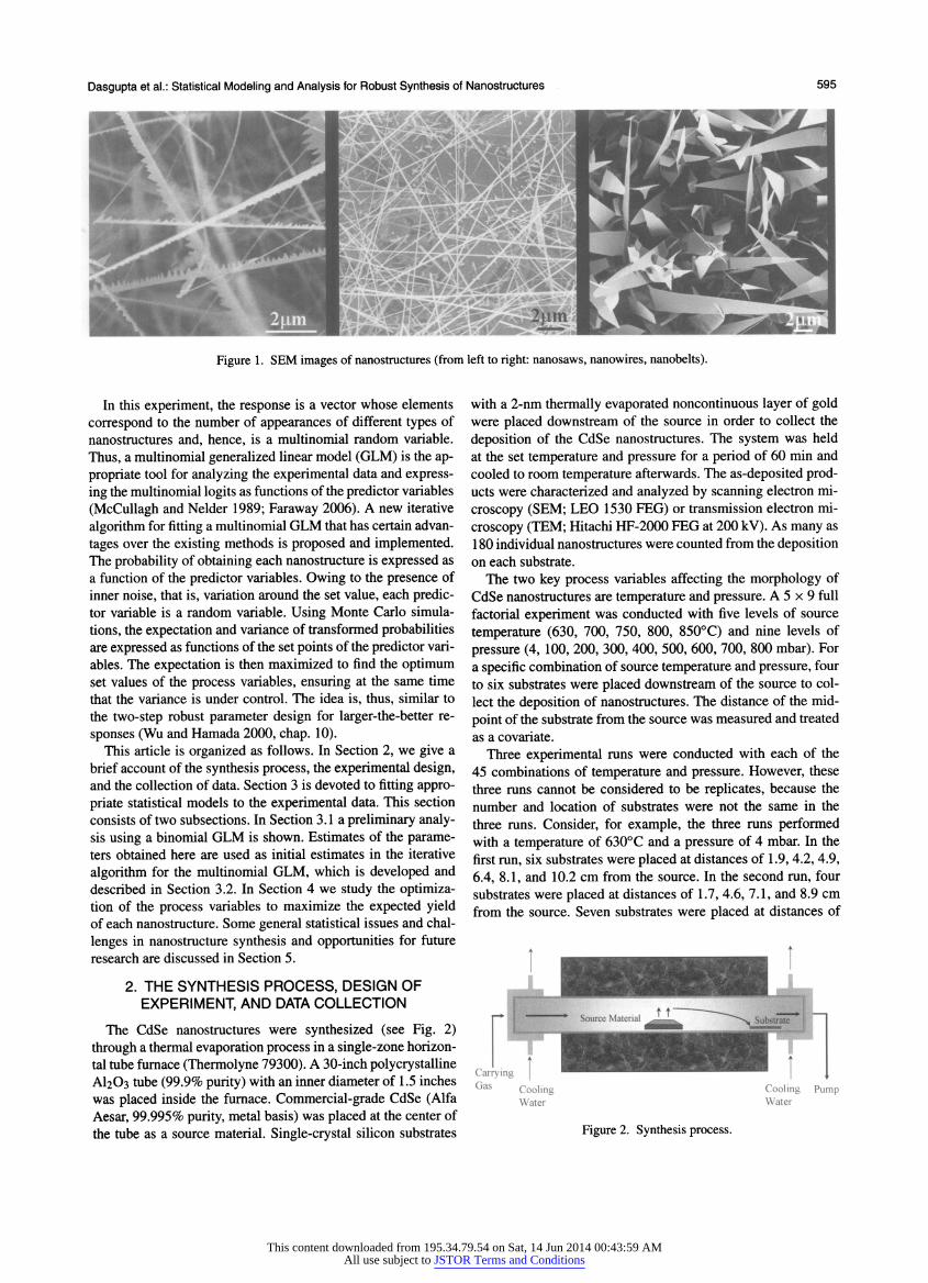
range of nanoscale processes. CdSe is found to exhibit the one

dimensional morphologies of nanowires, nanobelts, and nano

saws (Ma and Wang 2005), often with the three morphologies being intimately intermingled within the as-deposited material.

Images of these three nanostructures obtained using a scanning electron microscope are shown in Figure 1.

? 2008 American Statistical Association Journal of the American Statistical Association

June 2008, Vol. 103, No. 482, Applications and Case Studies DOI 10.1198/016214507000000905

594



Dasgupta et al.: Statistical Modeling and Analysis for Robust Synthesis of Nanostructures

Figure 1. SEM images of nanostructures (from left to right: nanosaws,

595

wires, nanobelts).

In this experiment, the response is a vector whose elements

correspond to the number of appearances of different types of nanostructures and, hence, is a multinomial random variable.

Thus, a multinomial generalized linear model (GLM) is the ap

propriate tool for analyzing the experimental data and express

ing the multinomial logits as functions of the predictor variables

(McCullagh and Neider 1989; Faraway 2006). A new iterative

algorithm for fitting a multinomial GLM that has certain advan

tages over the existing methods is proposed and implemented. The probability of obtaining each nanostructure is expressed as a function of the predictor variables. Owing to the presence of inner noise, that is, variation around the set value, each predic tor variable is a random variable. Using Monte Carlo simula

tions, the expectation and variance of transformed probabilities are expressed as functions of the set points of the predictor vari

ables. The expectation is then maximized to find the optimum set values of the process variables, ensuring at the same time that the variance is under control. The idea is, thus, similar to

the two-step robust parameter design for larger-the-better re

sponses (Wu and Hamada 2000, chap. 10). This article is organized as follows. In Section 2, we give a

brief account of the synthesis process, the experimental design, and the collection of data. Section 3 is devoted to fitting appro

priate statistical models to the experimental data. This section

consists of two subsections. In Section 3.1 a preliminary analy sis using a binomial GLM is shown. Estimates of the parame ters obtained here are used as initial estimates in the iterative

algorithm for the multinomial GLM, which is developed and

described in Section 3.2. In Section 4 we study the optimiza tion of the process variables to maximize the expected yield of each nanostructure. Some general statistical issues and chal

lenges in nanostructure synthesis and opportunities for future

research are discussed in Section 5.

2. THE SYNTHESIS PROCESS, DESIGN OF EXPERIMENT, AND DATA COLLECTION

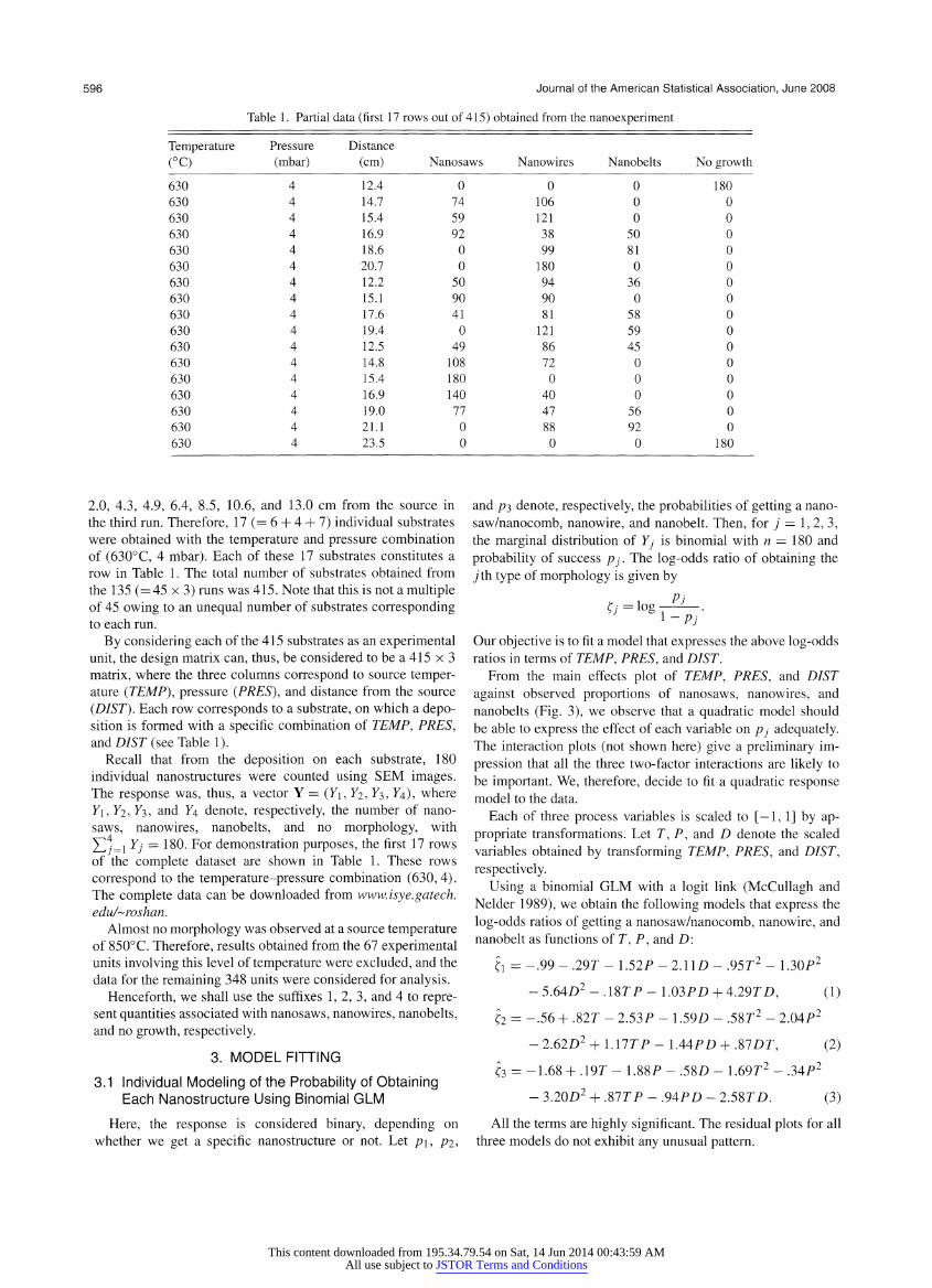
The CdSe nanostructures were synthesized (see Fig. 2)

through a thermal evaporation process in a single-zone horizon tal tube furnace (Thermolyne 79300). A 30-inch polycrystalline AI2O3 tube (99.9% purity) with an inner diameter of 1.5 inches was placed inside the furnace. Commercial-grade CdSe (Alfa Aesar, 99.995% purity, metal basis) was placed at the center of the tube as a source material. Single-crystal silicon substrates

with a 2-nm thermally evaporated noncontinuous layer of gold were placed downstream of the source in order to collect the

deposition of the CdSe nanostructures. The system was held at the set temperature and pressure for a period of 60 min and

cooled to room temperature afterwards. The as-deposited prod

ucts were characterized and analyzed by scanning electron mi

croscopy (SEM; LEO 1530 FEG) or transmission electron mi

croscopy (TEM; Hitachi HF-2000 FEG at 200 kV). As many as

180 individual nanostructures were counted from the deposition on each substrate.

The two key process variables affecting the morphology of

CdSe nanostructures are temperature and pressure. A 5 x 9 full

factorial experiment was conducted with five levels of source

temperature (630, 700, 750, 800, 850?C) and nine levels of

pressure (4, 100, 200, 300, 400, 500, 600, 700, 800 mbar). For a specific combination of source temperature and pressure, four

to six substrates were placed downstream of the source to col lect the deposition of nanostructures. The distance of the mid

point of the substrate from the source was measured and treated as a covariate.

Three experimental runs were conducted with each of the

45 combinations of temperature and pressure. However, these

three runs cannot be considered to be replicates, because the

number and location of substrates were not the same in the

three runs. Consider, for example, the three runs performed with a temperature of 630?C and a pressure of 4 mbar. In the

first run, six substrates were placed at distances of 1.9,4.2, 4.9,

6.4, 8.1, and 10.2 cm from the source. In the second run, four

substrates were placed at distances of 1.7, 4.6, 7.1, and 8.9 cm

from the source. Seven substrates were placed at distances of

Cooling Cooling Pump Water Water

Figure 2. Synthesis process.



596 Journal of the American Statistical Association, June 2008

Table 1. Partial data (first 17 rows out of 415) obtained from the nanoexperiment

Temperature Pressure Distance

(?C) (mbar) (cm) Nanosaws Nanowires Nanobelts No growth

630 4 12.4 0 0 0 180 630 4 14.7 74 106 0 0

630 4 15.4 59 121 0 0 630 4 16.9 92 38 50 0 630 4 18.6 0 99 81 0 630 4 20.7 0 180 0 0 630 4 12.2 50 94 36 0 630 4 15.1 90 90 0 0 630 4 17.6 41 81 58 0 630 4 19.4 0 121 59 0 630 4 12.5 49 86 45 0 630 4 14.8 108 72 0 0

630 4 15.4 180 0 0 0 630 4 16.9 140 40 0 0 630 4 19.0 77 47 56 0 630 4 21.1 0 88 92 0

630 4 23.5 0 0 0 180

2.0, 4.3, 4.9, 6.4, 8.5, 10.6, and 13.0 cm from the source in

the third run. Therefore, 17 (= 6 + 4 + 7) individual substrates were obtained with the temperature and pressure combination

of (630?C, 4 mbar). Each of these 17 substrates constitutes a row in Table 1. The total number of substrates obtained from the 135 (=45 x 3) runs was 415. Note that this is not a multiple of 45 owing to an unequal number of substrates corresponding to each run.

By considering each of the 415 substrates as an experimental unit, the design matrix can, thus, be considered to be a 415 x 3

matrix, where the three columns correspond to source temper ature (TEMP), pressure (PRES), and distance from the source

(DIST). Each row corresponds to a substrate, on which a depo sition is formed with a specific combination of TEMP, PRES, and DIST (see Table 1).

Recall that from the deposition on each substrate, 180 individual nanostructures were counted using SEM images.

The response was, thus, a vector Y = (Y\, Yi, Y3,14), where

Y\,Y2,Yi, and Y4 denote, respectively, the number of nano

saws, nanowires, nanobelts, and no morphology, with

J2 j=\ Yj = 180. For demonstration purposes, the first 17 rows

of the complete dataset are shown in Table 1. These rows

correspond to the temperature-pressure combination (630,4).

The complete data can be downloaded from www.isye.gatech. edu/~roshan.

Almost no morphology was observed at a source temperature

of 850?C. Therefore, results obtained from the 67 experimental units involving this level of temperature were excluded, and the data for the remaining 348 units were considered for analysis.

Henceforth, we shall use the suffixes 1, 2, 3, and 4 to repre sent quantities associated with nanosaws, nanowires, nanobelts,

and no growth, respectively.

3. MODEL FITTING

3.1 Individual Modeling of the Probability of Obtaining Each Nanostructure Using Binomial GLM

Here, the response is considered binary, depending on whether we get a specific nanostructure or not. Let p\, pi,

and /?3 denote, respectively, the probabilities of getting a nano

saw/nanocomb, nanowire, and nanobelt. Then, for j = 1, 2, 3,

the marginal distribution of Yj is binomial with n = 180 and

probability of success pj. The log-odds ratio of obtaining the

yth type of morphology is given by

Our objective is to fit a model that expresses the above log-odds ratios in terms of TEMP, PRES, and DIST.

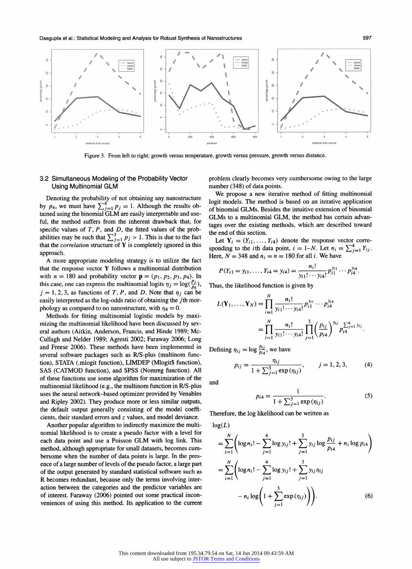
From the main effects plot of TEMP, PRES, and DIST

against observed proportions of nanosaws, nanowires, and

nanobelts (Fig. 3), we observe that a quadratic model should be able to express the effect of each variable on pj adequately. The interaction plots (not shown here) give a preliminary im

pression that all the three two-factor interactions are likely to be important. We, therefore, decide to fit a quadratic response

model to the data.

Each of three process variables is scaled to [?1, 1] by ap propriate transformations. Let T, P, and D denote the scaled

variables obtained by transforming TEMP, PRES, and DIST,

respectively.

Using a binomial GLM with a logit link (McCullagh and Neider 1989), we obtain the following models that express the

log-odds ratios of getting a nanosaw/nanocomb, nanowire, and

nanobelt as functions of T, P, and D:

?x = -.99

- .297

- 1.527

- 2.11D

- .95T2

- 130P2

- 5.64D2 - .1877 - 1.03PD + 4.29TD, (1)

l2 = -.56 + .827

- 2.537

- 1.59D

- .5872

- 2.0472

- 2.62D2 + \.\1TP - \MPD + .877)7, (2)

?3 = -1.68 + .197

- 1.887

- .587>

- 1.6972

- .3472

- 3.20D2 + .8777 - .9APD - 2.587D. (3)

All the terms are highly significant. The residual plots for all three models do not exhibit any unusual pattern.



Dasgupta et al.: Statistical Modeling and Analysis for Robust Synthesis of Nanostructures 597

Figure 3. From left to right: growth versus temperature, growth versus pressure, growth versus distance.

3.2 Simultaneous Modeling of the Probability Vector

Using Multinomial GLM

Denoting the probability of not obtaining any nanostructure

by P4, we must have 5Zt=i Pj = * Although the results ob

tained using the binomial GLM are easily interpretable and use

ful, the method suffers from the inherent drawback that, for

specific values of 7, 7, and D, the fitted values of the prob abilities may be such that

J2j=\ Pj > 1- Trris is due to the fact that the correlation structure of Y is completely ignored in this

approach. A more appropriate modeling strategy is to utilize the fact

that the response vector Y follows a multinomial distribution with n = 180 and probability vector p = (p\,pi, P3, P4). In this case, one can express the multinomial logits rjj

= log(^?),

j = 1,2,3, as functions of 7, 7, and D. Note that rjj can be

easily interpreted as the log-odds ratio of obtaining the y th mor

phology as compared to no nanostructure, with 774 = 0. Methods for fitting multinomial logistic models by maxi

mizing the multinomial likelihood have been discussed by sev

eral authors (Aitkin, Anderson, Francis, and Hinde 1989; Mc

Cullagh and Neider 1989; Agresti 2002; Faraway 2006; Long and Freese 2006). These methods have been implemented in several software packages such as R/S-plus (multinom func

tion), STATA (.mlogit function), LIMDEP (Mlogit$ function), SAS (CATMOD function), and SPSS (Nomreg function). All of these functions use some algorithm for maximization of the multinomial likelihood (e.g., the multinom function in R/S-plus uses the neural network-based optimizer provided by Venables and Ripley 2002). They produce more or less similar outputs, the default output generally consisting of the model coeffi

cients, their standard errors and z values, and model deviance.

Another popular algorithm to indirectly maximize the multi nomial likelihood is to create a pseudo factor with a level for each data point and use a Poisson GLM with log link. This

method, although appropriate for small datasets, becomes cum

bersome when the number of data points is large. In the pres ence of a large number of levels of the pseudo factor, a large part of the output generated by standard statistical software such as

R becomes redundant, because only the terms involving inter

action between the categories and the predictor variables are

of interest. Faraway (2006) pointed out some practical incon veniences of using this method. Its application to the current

problem clearly becomes very cumbersome owing to the large number (348) of data points. We propose a new iterative method of fitting multinomial

logit models. The method is based on an iterative application of binomial GLMs. Besides the intuitive extension of binomial GLMs to a multinomial GLM, the method has certain advan

tages over the existing methods, which are described toward the end of this section.

Let Y,- =

(F/i,..., F/4) denote the response vector corre

sponding to the ith data point, i = l-N. Let n? = EJ=i Yij Here, N = 348 and m = n = 180 for all i. We have

P(r?i=y?i,...,r?4 = yi4)= "/!

rf? - - -

p?? .

Thus, the likelihood function is given by

L(YU...,YN) = Y\ ,"'' .jfl'-jff

~l\y^-yi4il\{piJ Pi*

Defining rjij = log ̂-,

we have

PU = , . v^3 , ,? J = l>2' 3> W

1 + Ey=i expiry) and

#4 =-?0- (5) 1 + Ey=i?p(ity)

Therefore, the log likelihood can be written as

log(L)

= ]T( log?/;!

- ?]logyz7! + ]^y,7 log

? + n,- \ogpiA )

AT / 4 3

=Yl[l?znil~J2log ̂ !+J2 yiJ vu i=l \ 7=1 ;=1

- n? log! 1 + J^exp(n/7) 11. (6)




Let x, - (hTitPitDi^^P^Df^iPi^iDitTiDi)', i =

1,..., N. The objective is to express the 77's as functions of x.

Substituting T]ij =

x't?j in (6) and successively differentiating

with respect to each ?j,we get the maximum likelihood (ML)

equations as

i + E,-=iexP0?<7)/ ;=i

(7)

V x, yu -

m-?3- = 0, (8)

where 0 denotes a vector of 0's having length 10. Writing exp(y//) = (1 + Y<jjki cxp(rjij))~l, we obtain from (7)

Tjyij-ni ?P^ + ̂ > W 7 = 1,2,3. (9)

Note that each equation in (9) is the ML equation of a bi nomial GLM with logit link. Thus, if some initial estimates of

?2, ?i are available and, consequently, yu can be computed,

then ?x can be estimated by fitting a binomial GLM of Y\ on x.

Similarly, ?2 and ?3 can be estimated. The following algorithm is, thus, proposed.

Binomial GLM-Based Iterative Algorithm for Fitting a

Multinomial GLM. Let ?{p

be the estimate of ?j, j = 1, 2, 3, at the end of the kth iteration.

Step 1. Using ?(2k) and ?f], compute rj^ =

^?2k) and ?(*) ~/a(*)

l+exp(^)+exp(^3J)' Step 2. Compute y.f

= log m' ,?(*v ' = *'

Step J. Treating Y\ as the response and using the same de

sign matrix, fit a binomial GLM with logit link. The

vector of coefficients thus obtained is ? \ Step 4. Repeat Steps 1-3 by successively updating y\2 and

y?3 and estimating ?2 and ?3

Repeat Steps 1-4 until convergence. A proof of convergence is

given in Appendix A. Note that we use the "offset" command in the statistical software R to separate the coefficients associated

with 771 from those with y\.

To obtain the initial estimates ryi2 and ̂3 , we use the results obtained from the binomial GLM as described in Section 4.1. Let

iog-^ = x;?;, (io)

1 - no

where 8j is obtained using binomial GLM. Recalling the defin ition of r)ij, we get the initial estimates

-<0) _ w_Pi?

l-E/=lPi7 ffi=log ^ ^ , 7=2,3, (11)

where p~n, I = 1,2,3, are estimated from (10). It is possible,

however, that, for some /, ̂/=1 p~n = 7ti > 1. For those data

points, we provide a small correction as follows:

'^(l-?Y / = 1.2,3 ~

I 1

where /^ denotes the corrected estimated probability. To jus tify the correction, we note that it is a common practice to give a

correction of ̂- (Cox 1970, chap. 3) in the estimation of prob abilities from binary data. The correction given to category 4 is

adjusted among the other three categories in the same propor

tion as the estimated probabilities. This ensures that pn > 0 for all i and J2i=\ Pu ? 1

In this example, there were 18 data points (out of 348) cor

responding to which we had J2i=\ P~u ? 1- Following the pro cedure described previously to obtain the initial estimates, the

following models were obtained after convergence:

fn = A2- .127 - 3.08P - 3.68D - 1.8472 - 1.52P2

- 9.09D2 + .60TP - 2.31 PD + 5.15TD, (12)

fn = -54 + .887 - 3.S5P - 3.13D - 1.2172 - 2.28P2

- 5.26D2 + 1.S3TP - 2.62PD + 2.07TD, (13)

% = -.10 + .397 - 3.67 P - 2.51/) - 2.5172 - 1.12P2

- 7.07D2 + 1.12TP - 2.38PD + AA1TD. (14)

Inference for the Proposed Method. To test the significance of the terms in the model, one can use the asymptotic nor

mality of the maximum likelihood estimates. Let H? denote the 30 x 30 matrix consisting of the negative expectations of second-order partial derivatives of the log-likelihood function in (6), the derivatives being taken with respect to the compo nents of ?Y, ?2, and ?3. By denoting the final estimator of ? as ?*, the estimated asymptotic variance-covariance matrix of

the estimated model coefficients is given by T?* = H7*. For

a specific coefficient ?\, the null hypothesis Hq : ?i = 0 can be

tested using the test statistic z = ?i/s(?i), where s2(?i) is the Zth diagonal element of X^*.

Let ?f denote the estimate of ?\ obtained after the kth

iteration of the proposed algorithm. Let s2(?\ ) denote the

estimated asymptotic variance of ?\ . It can easily be seen

(App. B) that s2(?j ) converges to s2(?*). Thus, as the para meter estimates converge to the maximum likelihood estimates,

their standard errors also converge to the standard error of the

MLE. More generally, if Ha?) denotes the asymptotic covari

ance matrix of the parameter estimates at the end of the &th

iteration, then T,o(k) ?> ??*.

The preceding property of the proposed algorithm ensures that one does not have to spend any extra computational effort

in judging the significance of the model terms. The binomial GLM function in R used in every iteration automatically tests the significance of the model terms, and the p values associated

with the estimated coefficients after convergence can be used

for inference. Thus, the inferential procedures and diagnostic tools of the binomial GLM can easily be used in the multino

mial GLM model. This is clearly an advantage of the proposed algorithm over existing methods. Further, the three models for

nanosaws, nanobelts, and nanowires can be compared using




Table 2. p value for each estimated coefficient

Nanosaws (r?\) Nanowires (rfe) Nanobelts (^3)

Term ? S.E. p value ? S.E. p value ? S.E. p value

Intercept .42 .24 .0807 .54 .25 .0343 -.10 .24 .6763

7 -.12 .30 .6855 .88 .28 .0020 .39 .38 .3125

P -3.08 .41 .0000 -3.85 .50 .0000 -3.67 .51 .0000

D -3.69 .67 .0000 -3.13 .57 .0000 -2.51 .66 .0001

F2 -1.84 .34 .0000 -1.21 .27 .0000 -2.51 .34 .0000

P2 -1.52 .44 .0006 -2.28 .52 .0000 -1.12 .54 .0381

D2 -9.09 .99 .0000 -5.26 .66 .0000 -7.08 .77 .0000

77 .60 .42 .1515 1.83 .41 .0000 1.72 .53 .0011

PD -2.31 .83 .0053 -2.62 .70 .0000 -2.38 .84 .0043

FD 5.75 .80 .0000 2.07 .45 .0000 4.47 .69 .0000

these diagnostic tools. Such facilities are not available in the current implementation of other software packages.

In the fitted models given by (12)?(14), all 30 coefficients are seen to be highly significant with p values on the order of 10~6 or less. To check the model adequacy, we use the gen

eralized R2 statistic derived by Naglekerke (1991) defined as R2 = (1

- exp((D

- Dnuii)/rt))/(l

- exp(-Dnuii/?)), where

D and Dnun denote the residual deviance and the null deviance,

respectively. The R2 associated with the models for nanosaws, nanowires, and nanobelts are obtained as 61%, 50%, and 76%,

respectively. This shows that the prediction error associated

with the model for nanowires is the largest. This finding is con sistent with the observation made by Ma and Wang (2005) that

growth of nanowires is less restrictive compared to that of nano

saws and nanowires and can be carried out over wide ranges of

temperature and pressure.

However, the small p values may also arise from the fact

that some improper variance is used in testing. This overdis

persion may be attributed to either some correlation among the

outcomes from a given run in the experiment or some unex

plained heterogeneity within a group owing to the effect of some unobserved variable. A multitude of external noise fac

tors in the system make the second reason a more plausible one. We re-perform the testing by introducing three dispersion parameters a2, a2, and a2, which are estimated from the ini

tial binomial fits using (7? = x?/(N? 10), where y2 denotes

Pearson's x2 statistic for the jth nanostructure, j =

1, 2, 3, and

N ?10 = 338 is the residual degrees of freedom. The estimated standard errors of the coefficients and the corresponding p val

ues are shown in Table 2.

From Table 2, we find that the linear effect of temperature is not significant for nanosaws and nanobelts. However, because

the quadratic term T2 and the interactions involving T are sig nificant, we prefer to retain T in the models.

Note that although techniques for analyzing overdispersed binomial data are well known (e.g., Faraway 2006, chap. 2),

methods for handling overdispersion in multinomial logit mod els are not readily available. The proposed algorithm provides us with a very simple heuristic way to do this and, thereby, has an additional advantage over the existing methods.

4. OPTIMIZATION OF THE SYNTHESIS PROCESS

In the previous sections, the three process variables have

been treated as nonstochastic. However, in reality, none of these

variables can be controlled precisely, and each of them exhibits certain fluctuations around the set (nominal) value. Such fluctu

ation is a form of noise, called internal noise (Wu and Hamada

2000, chap. 10), associated with the synthesis process and needs to be considered in performing optimization.

It is, therefore, reasonable to consider TEMP, PRES, and

D1ST as random variables. Let /?temp, I^pres, and ?Disr de

note the set values of TEMP, PRES, and DIST, respectively. Then we assume

TEMP^N(?TEMP,cr2EMP),

PRES ~ N(?pREs, VpRES^

DIST^N(?DIsT,c>2IST),

where OjEMP, <JpRES, and (y^IST

are the respective variances of

TEMP, PRES, and DIST around their set values and are esti mated from process data (Sect. 5.1). The task now is to deter

mine the optimal nominal values of ?jltemp, ?PRES, and /jldist

so that the expected yield of each nanostructure is maximized

subject to the condition that the variance in yield is acceptable.

4.1 Measurement of Internal Noise in the

Synthesis Process

Some surrogate process data collected from the furnace were

used for estimation of the preceding variance components.

Temperature and pressure were set at specific levels (those used

in the experiment), and their actual values were measured re

peatedly over a certain period of time. The range of tempera ture and pressure corresponding to each set value was noted.

The variation in distance, which is due to repeatability and re

producibility errors associated with the measurement system,

was assessed separately. The summarized data in Table 3 show

the observed ranges of TEMP, PRES, and DIST against dif ferent nominal values. Under the assumption of normality, the

range can be assumed to be approximately equal to six times

the standard deviation.

We observe from Table 3 that, for the process variable DIST, the range of values around the nominal ?jldist is constant (2 x

.02 = .04 cm) and independent of ?jldist- Equating this range to

6&disf, we obtain an estimate of odist as .04/6 = .067 cm.

Similarly, for TEMP, the range can be taken to be almost a constant. Equating the mean range of 12.8 (=2 x (2 x 7 +




Table 3. Fluctuation of process parameters around set values

Temperature (?C)

Nominal value

(Mr)

630 700 750 800 850

Observed range

(*?3crT)

?7 ?7 ?6 ?6 ?6

Pressure (mbar) Distance (cm)

Nominal value

(PP)

4 100 200 300 400 500 600

Observed range

(-?3ap)

?10 ?10 ?20 ?20 ?20 ?40 ?40

Nominal value

(pd)

11 13 15 17 19 21

Observed range

(- ?3aD)

?.02

?.02

?.02

?.02

?.02

?.02

3 x 6)/5)?C to 6apEMP, an estimate of gjemp is obtained as

12.8/6 = 2.13?C. The case of PRES is, however, different. The range, and

hence opr?s, 1S an increasing function of ppres- Correspond

ing to each value of ppres, an estimate of a pr?s is obtained by dividing the range by 6. Using these values of a pr?s, the fol

lowing regression line is fitted through the origin to express the

relationship between a pr?s and ppres'

&PRES = 025 ?PRES (15)

Recall that all the models are fitted with the transformed vari ables T, P, and D. The means pj,pp, and pp> and the vari

ances Gj,o2 and a? can easily be expressed in terms of the

respective means and variances of the original variables.

4.2 Obtaining the Mean and Variance Functions of pi,p2, andp3

From (4), we can write the estimated probability functions

&spj =

Qxip(ffj)/(\ + X!/=i exP(*7)))> where ry are given by (12)-(14).

Expressing E(pj) and Var(/?7) in terms of pj,pp, and

po is not a straightforward task. To do this, we use Monte Carlo simulations. For each of the 180 combinations of ?jltemp, Ppres, and pdist (??temp = 630, 700, 750, and 800?C; Ppres = 4, 100, 200,..., 800 mbar; pDIST = 12, 14, 16, 18, and 20 cm), the following are done:

1. pt, pp, and po are obtained by appropriate transforma

tion.

2. Five thousand observations on T, P, and D are gener

ated from the respective normal distributions and rjj is obtained using (12), (13), or (14).

3. From the rjj values thus obtained, p/s are computed us

ing (4) and transformed to ?j =

\og(pj/(l ?

pj)). 4. The mean and variance of those 5,000 ?j values [denoted

by ?j and s2(?j), respectively] are computed. 5. Using linear regression, ?j and \ogs2(?j) are expressed in

terms of pp, Pp, and po

4.3 Maximizing the Average Yield

Because the response here is of larger-the-better type, max

imizing the mean is more important than minimizing the vari ance in the two-step optimization procedure (Wu and Hamada

2000, chap. 10) associated with robust parameter design.

The problem can thus be formulated as

Maximize ?j subject to ? 1 < /?p < 1, ? 1 < /?p < L

-1 <?D< lfor j = 1,2,3.

Physically, this would mean maximizing the average log-odds ratio of getting a specific morphology.

The following models are obtained from the simulated data:

Y\ = -.75 + .20/zp

- 1.02/xp

- 1.39/xz)

- 1.50/4

- 3.54/4

- 11.02/4 + 1.58/xr/xp

- 2.22\ip\iD + 8.41/zp/?p>, (16)

& = -.40 + .80/?p

- 2.96/xp

- 1.43/x/)

- .98/4

- 2.45/4

- 6.05/4 + 1.87/zrMP

- 3Al?p?p + 2A3?T?D, (17)

?3 = ?1.25 + .26/xp

? 2.6/xp

? .42/xp>

? 2.36?jlt

- 1.24/4

- 8.03/4 + 1.74/xp/xp

- 3.32/?p/xD + 4.57/xp/XD- (18)

Maximizing these three functions using the o/?i/m command in R, we get the optimal conditions for maximizing the expected yield of nanosaws, nanowires, and nanobelts in terms of /xp,

ftp, and ?ip). These optimal values are transformed to the orig inal units (i.e., in terms of ?jltemp, I^pres, and ?xdist) and are summarized in Table 4.

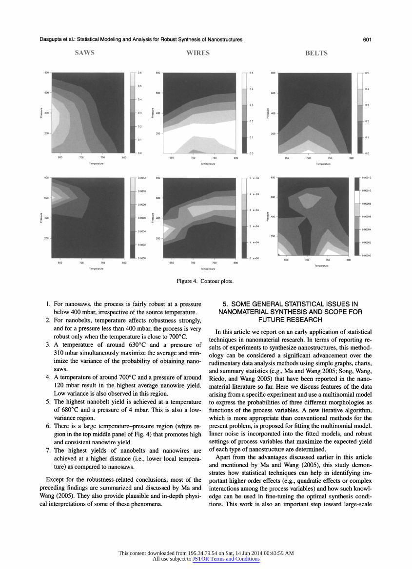
Contour plots of the average and variance of the yield proba bilities of nanosaws, nanowires, and nanobelts against temper ature and pressure (at optimal distances) are shown in Figure 4. The white regions on the top (average) panels and the black re

gions on the bottom (variance) panels are robust regions that

promote high yield with minimal variation. On the basis of these contour plots and the optimization out

put summarized in Table 4, the following conclusions can be drawn:

Table 4. Optimal process conditions for maximizing the expected

yield of nanostructures

Nanostructure Temperature (?C) Pressure (mbar) Distance (cm)

Nanosaws 630 307 15.1

Nanowires 695 113 19.0

Nanobelts 683 4 17.0



Dasgupta et al.: Statistical Modeling and Analysis for Robust Synthesis of Nanostructures

SAWS WIRES BELTS

601

TOO 750

5 ?-04 MO

Figure 4. Contour plots.

1. For nanosaws, the process is fairly robust at a pressure below 400 mbar, irrespective of the source temperature.

2. For nanobelts, temperature affects robustness strongly, and for a pressure less than 400 mbar, the process is very robust only when the temperature is close to 700?C.

3. A temperature of around 630? C and a pressure of 310 mbar simultaneously maximize the average and min imize the variance of the probability of obtaining nano saws.

4. A temperature of around 700?C and a pressure of around 120 mbar result in the highest average nanowire yield.

Low variance is also observed in this region. 5. The highest nanobelt yield is achieved at a temperature

of 680? C and a pressure of 4 mbar. This is also a low variance region.

6. There is a large temperature-pressure region (white re

gion in the top middle panel of Fig. 4) that promotes high and consistent nanowire yield.

7. The highest yields of nanobelts and nanowires are

achieved at a higher distance (i.e., lower local tempera ture) as compared to nanosaws.

Except for the robustness-related conclusions, most of the

preceding findings are summarized and discussed by Ma and

Wang (2005). They also provide plausible and in-depth physi cal interpretations of some of these phenomena.

5. SOME GENERAL STATISTICAL ISSUES IN NANOMATERIAL SYNTHESIS AND SCOPE FOR

FUTURE RESEARCH

In this article we report on an early application of statistical

techniques in nanomaterial research. In terms of reporting re sults of experiments to synthesize nanostructures, this method

ology can be considered a significant advancement over the

rudimentary data analysis methods using simple graphs, charts, and summary statistics (e.g., Ma and Wang 2005; Song, Wang, Riedo, and Wang 2005) that have been reported in the nano material literature so far. Here we discuss features of the data

arising from a specific experiment and use a multinomial model to express the probabilities of three different morphologies as functions of the process variables. A new iterative algorithm, which is more appropriate than conventional methods for the

present problem, is proposed for fitting the multinomial model. Inner noise is incorporated into the fitted models, and robust

settings of process variables that maximize the expected yield of each type of nanostructure are determined.

Apart from the advantages discussed earlier in this article and mentioned by Ma and Wang (2005), this study demon strates how statistical techniques can help in identifying im

portant higher order effects (e.g., quadratic effects or complex interactions among the process variables) and how such knowl

edge can be used in fine-tuning the optimal synthesis condi tions. This work is also an important step toward large-scale




controlled synthesis of CdSe nanostructures, because in addi

tion to determining conditions for high yield, it also identifies robust settings of the process variables that are likely to guar antee consistent output.

Although statistical design of experiments (planning, analy sis, and optimization) has been applied very successfully to various other branches of scientific and engineering research

to determine high-yield and reproducible process conditions, its application in nanotechnology has been limited to date. Some unique aspects associated with the synthesis of nanos

tructures that make application of the preceding techniques in this area challenging are (i) complete disappearance of nanos

tructure morphology with slight changes in process conditions; (ii) complex response surface with multiple optima, making exploration of optimal experimental settings very difficult (al though in the current case study, a quadratic response surface

was found more or less adequate, such is not the case in gen

eral); (iii) different types of nanostructures (saws, wires, belts) intermingled; (iv) categorical response variables in most cases;

(v) functional inputs (control factors that are functions of time); (vi) a multitude of internal and external noise factors heavily affecting reproducibility of experimental results; and (vii) ex

pensive and time-consuming experimentation. In view of these

phenomena, the following are likely to be some of the ma

jor statistical challenges in the area of nanostructure synthe sis:

1. Developing a sequential space-filling design for maxi

mization of yield. Fractional factorial designs and orthog onal arrays are the most commonly used (Wu and Hamada

2000) designs, but are not suitable for nanomaterial syn thesis, because the number of runs becomes prohibitively

large as the number of levels increases. Moreover, they do

not facilitate sequential experimentation, which is neces

sary to keep the run size to a minimum. Response surface

methodology (Myers and Montgomery 2002) may not be useful because the underlying response surface encoun

tered in nanoresearch can be very complex with multi

ple local optima, and the binary nature of data adds to the complexity. Space-filling designs such as Latin hy percube designs, uniform designs, and scrambled nets are

highly suitable for exploring complex response surfaces with a minimum number of runs. They are now widely used in computer experimentation (Santner, Williams, and

Notz 2003). However, they are used in the literature for

only one-time experimentation. We need designs that are

model independent, quickly "carve out" regions with no

observable nanostructure morphology, allow for the ex

ploration of complex response surfaces, and can be used

for sequential experimentation. 2. Developing experimental strategies where one or more of

the control variables is a function of time. In experiments for nanostructure synthesis, there are factors whose pro

files or curves with respect to time are often crucial with

respect to the output. For example, although the peak tem

perature is a critical factor, how this temperature is at

tained over time is very important. There is an ideal curve that is expected to result in the best performance. Plan

ning and analysis of experiments with such factors (which are called functional factors) are not discussed much in

the literature and may be an important topic for future re

search.

3. Scale-up. One of the important future tasks of the nan

otechnology community is to develop industrial-scale manufacture of the nanoparticles and devices that are

rapidly being developed. This transition from laboratory level synthesis to large-scale, controlled, and designed

synthesis of nanostructures poses plenty of challenges. The key issues to be addressed are rate of production, process capability, robustness, yield, efficiency, and cost.

The following specific tasks may be necessary: (1) deriv

ing specifications for key quality characteristics of nanos tructures based on intended usage [quality loss functions

(Joseph 2004) may be used for this purpose]; (2) ex

panding the laboratory setup to simulate additional condi tions that are likely to be present in an industrial process; (3) conducting experiments and identifying robust set

tings of the process variables that will ensure manufactur

ing of nanostructures of specified quality with high yield; and (4) statistical analysis of experimental data to com

pute the capability of the production process with respect to each quality characteristic.

APPENDIX A: PROOF OF CONVERGENCE OF THE PROPOSED ALGORITHM

For simplicity, consider a single predictor variable and assume that

rjij =

?jXj, where

?j is a scalar (/ = 1, 2, ..., N, j

= 1, 2, 3). Let

Q(?l, ft, ft) = E,l, (? =, yuVij

- n? log(l + Ly=i expfo,;))) Recall that ?

. denotes the estimate of ?j obtained after the kth J J

iteration. Then it suffices to show that (i) Q(?\, ?2, ?i) is a con

cave function of ?j, j = 1,2,3, and (ii) Q(?[M), ?2\ ?f]) >

?(Pl .P2 'P3 ) It is easy to see that, for / = 1, 2, 3,

92Q _ N n.x2e?m (! + E .^ g?jXi ) ̂ ^

W? ~

hi (l+?j=1^')2 which proves the concavity of Q.

(k) (k) To prove (ii), we note that, for given ?) , ?\ , the solution for ?\ in the equation

N ? 1 R{k)v

/=iv i + ??^+?j=2e'

maximizes Q(?h ?^], ?(/}). From the first equation of (9) and Steps 1-3 of the algorithm, we

have

which means ?\'

= arg max Q(?\, ?\ > ?\ ) Therefore, (ii) holds.

APPENDIX B: PROOF OF CONVERGENCE OF THE ESTIMATED COVARIANCE MATRIX

Again, for simplicity, consider a single predictor variable and as

sume that rjij =

?jX[, where

?j is a scalar (/ = 1, 2,..., N, j

=

(k) 1, 2, 3). Let ? denote the estimate of

?j obtained after Steps 1-3




of the kth iteration and let ?* denote the final estimate of ?j obtained J J

by the proposed algorithm. (k) ? (k) The estimated asymptotic variance of ?j , denoted by s (?\ ),

is given by the negative expectation of ??K lA

\ {k) {k-\) ?(k-\), ?P] P\ 'Pi 'P3

where logL^ denotes the binomial log-likelihood function of y?\, i = 1,..., N, that corresponds to the first of the three equations in (9) and is given by

N / x N

log?M =^]log( w

)+5^yn(^T+y/T) 1 = 1 1 = 1

N

-?z-^log(l+exp(^i +y/i)). ;=i

Now, s2(?*), the estimated asymptotic variance of ?*, is given by

the negative expectation of ?f \?.=?* 7 = i 2 3, where logL is the op, ^J "F

' '

multinomial likelihood given by (6). It can easily be seen that

d2\ogLb] _ y^ 2 l+expfa-2)+exp(TO)

d?2 ~

"f^ (l+exp(^1) + exp(^2)+exp(^3))2

_ 32logL

By convergence of ? to ?* for j = 1,2,3, it follows that

s2{?f))-^s2(?\). Similarly, each component in the covariance matrix L^) can be

proven to converge to each component of ??*.

[Received June 2006. Revised February 2007.]

REFERENCES

Agresti, A. (2002), Categorical Data Analysis, New York: Wiley. Aitkin, M., Anderson, D. A., Francis, B. J., and Hinde, J. P. (1989), Statistical

Modelling in GLIM, Oxford, U.K.: Clarendon Press.

Bawendi, M. G., Kortan, A. R., Steigerwald, M. L., and Brus, L. E. (1989), "X-Ray Structural Characterization of Larger Cadmium Selenide (CdSe) Semiconductor Clusters," Journal of Chemical Physics, 91, 7282-7290.

Cox, D. R. (1970), Analysis of Binary Data, London: Chapman & Hall.

Faraway, J. J. (2006), Extending the Linear Model With R: Generalized Lin

ear, Mixed Effects and Nonparametric Regression Models, Boca Raton, FL:

Chapman & Hall/CRC Press.

Hodes, G., Albu-Yaron, A., Decker, F., and Motisuke, P. (1987), "Three Dimensional Quantum-Size Effect in Chemically Deposited Cadmium Se lenide Films," Physics Review B, 36, 4215-4221.

Joseph, V. R. (2004), "Quality Loss Functions for Nonnegative Variables and Their Applications," Journal of Quality Technology, 36, 129-138.

Long, J. S., and Freese, J. (2006), Regression Models for Categorical Depen dent Variables Using Stata, College Station, TX: Stata Press.

Ma, C, and Wang, Z. L. (2005), "Roadmap for Controlled Synthesis of CdSe

Nanowires, Nanobelts and Nanosaws," Advanced Materials, 17, 1-6.

Ma, C, Ding, Y., Moore, D. F., Wang, X., and Wang, Z. L. (2004), "Single Crystal CdSe Nanosaws," Journal of the American Chemical Society, 126, 708-709.

McCullagh, P., and Neider, J. (1989), Generalized Linear Models, London:

Chapman & Hall.

Myers, H. M., and Montgomery, D. C. (2002), Response Surface Methodology: Process and Product Optimization Using Designed Experiments, New York:

Wiley. Naglekerke, N. (1991), "A Note on a General Definition of the Coefficient of

Determination," Biometrika, 78, 691-692.

Santner, T. J., Williams, B. J., and Notz, W. I. (2003), The Design and Analysis of Computer Experiments, New York: Springer-Verlag.

Song, J., Wang, X., Riedo, E., and Wang, Z. L. (2005), "Systematic Study on

Experimental Conditions for Large-Scale Growth of Aligned ZnO Nanowires on Nitrides," Journal of Physical Chemistry B, 109, 9869-9872.

Venables, W. N., and Ripley, B. D. (2002), Modern Applied Statistics With

S-PLUS, New York: Springer-Verlag. Wu, C. F. J., and Hamada, M. (2000), Experiments: Planning, Analysis, and

Parameter Design Optimization, New York: Wiley.



statistical modeling and analysis for robust synthesis of nanostructures

Documents