statistical methods for environmental pollution monitoring · pdf filestatistical methods for...

Statistical Methods for Environmental

Pollution Monitoring

Richard 0 Gilbert Pacific Northwest Laboratory

Ddicarrdlo ~f~porenrsMa MargaretondDonoldIG i l k n

nilbwt is pinled on acid-Ire prpc 8 copyright0 1537 by John Wiley amp Sans Ins Allrights rewnnd

Pvblirhcd simuluncoudy in Canada

~ o p m a f t h i publication may beampaccd s u r d in smricval sysnm or tnnrmittd in any farma by any mcanrclce~oni mechanical pho~oeapyingmording scanttina w Mhawirc c i q t a s p r m i n d undnScelions I01 or 108 ofthe 1916 United Slaw CopyrightAct wilhml rirha ihr priorwrinenprmirion of ihc mbliahcr anuthonation amugh payment a1 thc

8ddruvdmUuPcrminionsDcpumunc John Wiley amp Smr 1ncW5 mid Avmuc New Y o 4 NY 10158M12 i212)850Mll lax (212) 8506m8 euro-Mail M-QWL~SYCOM

approptiaapusopy fee bUu Cowight Cl-ncccentcr m RarnuoalDrivr hnnaM A 01923 (978) lmfax (977504144 R-u to thc Pvhlitha fap r m i u i m Lould be

G i l M Richard0 memods m

Bibliogsphy p Includcr index

sraci~rica~ mvimnmmral ponution monitoring

I~ollaion-~nvirnnrnsnlal anpulsStarirtisa1 ~

Contents

11 Types and Objectives of Envimnmental Pollution Studies I I 12 Statistical Design and Analysis Pmblems 1 2 13 Overview of the Design and Analysis Pmeess 1 3 14 Summary 1 4

2 Sampling Environmental Populations 1 5

2 L Sampling in Space and Time 1 5 22 Target and Sampled Populations 1 7 23 Representative Units 9

-24 Choosing a Sam~line Plan I In~ 25 variability and Enor in Envimnmental Studies 1 LO 26 Case Study 1 13 27 Summary 1 15

3 Environmental Sampling Design 1 17

31 lntmduction 1 17 32 Criteria for Chmsiag a Sampling Plan 1 17 33 Methods for Selecting Sampling LoCaliations and Times 1 19 34 Summary 1 24

4 Simple Random Sampling 1 26

41 Basic Comeper 1 26 42 Eslimating tbe Mean and Total Amount 1 27 43 Effect of Measurement E m n 30 44 Number of Measurements Independent Data 1 30 45 Number of Mcasu~ments Conelated Data 35 46 Estimating VarO 1 42 47 Summary 1 4 3

5 Stratifled Random Sampling 1 45 c -

Types of Trends 205

Detecting and16 Estimating Fend

An imponant objective of many envimnmental monitoring pmgrams is to detect changes or trends in pollution levels over time The purpose may be to look far increased envimnmental pollution resulting fmm changing land use practices such as the gmwth of cities increased emsion fmm farmland into riven or the stanup of a hazardous waste storage facility Or the purpose may be to determine if pollution levels have declined following the initiation of pollution contml Droprams -

The Snt sections of this chapter dircu~s t ) p s of tmndr rtatistral complcr~tors in trend drtection graph~cal and regresston method$ 16 daccting and estimating tnnds and Box-lenkins lime scrics nlclhods for malcling polluliun pmrcsscs The remainder of the chapter describes the ~ann -~enda l i test for detecting monotonic vends at sinele or mult i~ lestations and Sens (18b) ~onnarametric esltmatur 01 trend (slope) Extenr~onsof the teclgtnques in t h~ r chapter to handle rcaronol etTects am gwen in Chapter I7 Append B lists a compatcr ccdc that computes the tests and trend estimates discussed in Chapten 16 and 17

161 TYPES OF TRENDS Figrrre 161 shows some common types of trends A sequence of measurements with no trend is shown in Figure IGl(a) The fluctuations along the sequence are due to random (unassignable) causes Figure 16l(b) illustrates a cyclical pattern wih no long-term trend and Figure IGl(c) shows random fluctuations I

I (C) TREND f NON-RANDOM I (0 RANDOM WITH IMPULSE

about s sing linear trend line Cycle may be caused by many factors induding seasonal dimatic changes tides changes in vehicle traffic patterns during the day pmduetion schedules of industry and so on Such cycles are not trends because they do not indicate long-term change Figure 16l(d) shows a cycle with a rising long-term trend with random fluctuation about the cycle

Frequently pollution measurements taken close together in time or space are positively conelated that is high (low) values are likely to be followed by

206 Detecting and Estimating Trends

treatment plant Finally a sequence of random measurements fluctuating about a constant level may be followed by a trend as shown in Figure 16L(h) We concenvatc here on tests for detecting monotonic increasing or d s m i n g trends as in (c) (dl (E) and (h)

162 STATISTICAL COMPLEXITIES The detection and estimation of uends is complicated by pmblems assaeiated with characteristics of pollution data In this tia an we review these problems m g g a appmaehes for Unir alleviation and reference pertinent literature for additional information Hamed d al (1981) review the literature dealing with mtistieal design and analysis aspects of detecting trends in water quality Munn (1981) reviews ~e thods for detecting trends in sir quality data

1621 Changes in Procedures A change of analytical laboratories or of sampling andor analytical pmeedum may occur during a long-term study Unfomnately this may cause a shift in the mean or in the variance of the measured values Such shifts could be inco-tly attributed to changes in the underlying natural or man-induced pmcesses generating the pollution

When changes in procedures or laboratories ocucr abruptly there may not be time to conduct comparative studies to estimate the magnitude of shifts due to these changes This pmblem can sometimes be avoided by preparing duplicate samples at the time of sampling one is analyzed and the other is stored to be analyzed if a change in laboratories or pmcedures is introduced later The paired old-new data on duplicate samples can then be compared for shifts or other inconsistencies This method assumes that the pollumts in the sample do not change while in storage an unrealistic assumption in many eases

1622 Seasonality The variation added by seasonal or other cycles makes it more difficult to detect long-term trends This problem can be alleviated by removing the cycle before applying tests or by using tests unaffected by cycles A simple nonparametric test for trend using the first approach was developed by Sen (1968a) The seasonal Kendall test discussed in Chapter 17 uses the latter appmach

1623 Correlated Data Pollution measurements taken in close proximity over time a n likely to be positively correlated but most statistical tests require uncamlated data One approach is to use test statistics developed by Sen (1963 1965) for dependent A- TO-- Oltgt --+a A -c eoet hd nes-rL

Methods 207

and pmvide tables of adjusted critical values for the Wilcoxon rank sum and Spearman tests Their paper summarizes the latest statistid techniquw for trend detection

1624 Corrections for Flow The detection of t ~ n d ~in stream water quality is more difficult when mncen-trations are dated to sueam flow Un usual situation Smith Hirseh and Slack (1982) obtain flow-adjusted wnanwtions by fitting a e o n equation to the mneentrafion-flow relationship Then he ampdads hom re-ion are tested for trend by the seasonal KendaU test discussed in Chapter 17 Hamed Daniel and Crawford (1981) illustrate two allemalive methcds discharge compensation and discharge-frequency weighting Methods for adjusting ambient air quality levels for meteomlogical effects an discussed by Zeldin and Meisel (1978)

163 METHODS

1631 Graphical Graphical methods are very useful aids to formal tests for trends The tint step is to plot the data against time of collection Velleman and Hoaglin (1981) provide a computer d e for this purpase which is designed for interactive ue an a computer terminal They also provide a computer code for smwthing time series to paint out cycles andlor long-term trends that may otherwise be obscured by variability in the data

Cumulative sum (CUSUM) charts are also an effective graphical tool With this method changes in the mean are d e t d by keeping a cumulative total of deviations fmm a reference value or of miduals from a rralistic stochastic model of the pmcess Page (1961 1963) Ewsn (1963) Gibra (1975) Wetherill (1977) Benhouex Hunter and Pallesen (1978) and Vardeman and David (1984) pmvide details on the method and additional refennces

1632 Regression If plats of data Venus time suggest a simple linear inercase or decrease over time a linear regression of the variable against time may be fit to the data A r test may be used to test that the tme slope is not different fmm mro see for example Snedecor and Cochran (1980 p 155) This Itest can be misleading if seasonal cycles are present the data are not normally distributed andlor the data are serially correlated Hirsch Slack and Smith (1982) show Ulat in t h s e situations the r test may indicate a significant slope when the uue slope actually is rero They also examine the performance of linear regression applied to deseasonalized data This procedure (called seasorto1 rqression) gave a r test

208 Defecting and Estimating Trends

1633 Intervention Analysis and Box- Jenkins Models

If a Ibng time rqucnce of equally spaced data is available intervention anrlyrir may be uwd to detect changer in average level rrsulttng fmm a natural or man-induced rntenentian in Lc pmces Thn approach developed by Box and Tiao (1975) is a generalization of the autoregressive integrated moving-avcrage (ARIMA) time series models d c s a i y by Box and Jenlrins (1976) Lett~maier and Murray (1977) and Lenenmaier (1978) study the power of the method to detect mnds They emphasize the design of sampling plans to detect impacts from polluting facilities Fxamples of its use are in Hipel et al (1975) and Roy and Pellerin (1982)

Box-Jenkins modeling techniques are powerful tools for the analysis of time series data McMiehael and Hunter (1972) give a gwd intductian to Box- Jenkins modeling bf envimnmental data using both deterministic and stochastic components to forecast temperature flow in the Ohio River Fuller and Tsokos (1971) develop models to forecast dissolved oxygen in a stnam Carlson MacConnick and Watts (1970) and MeKerchar and Delleur (1974) fit Box- Jenkins models to monthly river Rows Hsu and Hunter (1976) analyze annual series of-air pollution SO concentrations McCdlister and Wilson (1975) forecast daily maximum and hourly average total oxidant and carbon monoxide concen-trations in the Lm Aaples Basin Hipel McLmd and Lennor (19770 19776) illustrate impmved Box-Jenkins techniques to simplify model consmclion Reinsel et al (19810 19816) use Box-Jenkins models to detect trends in stratospheric omne data Two intductoty textbodrs are MeCleary and Hay (1980) and Chatfield (1984) Box and Jenkins (1976) is recommended reading for all users of the method

Disadvantages of Box-Jenkins methods are discussed by Montgomery and Johnson (1976) At least 50 and preferably LOO or more data collected at equal (or approximately equal) time intervals are needed When the purpose is forecasting we must assume the developed model applies to the future Missing data or data reported as trace or less-than values can prevent the use of Box- Jenkim methods Finally the modeling pmess is often nontrivial with a considerable inveslment in time and resources required to build a satisfactory~~ ~ ~~ ~~

model Fonunatcly them several packages of rtatnstiral prngramr that conlzin coder for developing time series models ineludmg Minitah (Ryan loincr and Ryan 1982) SPSS (1985) BMDP (1983) and SAS (1985) Codes for pcnonal computers are also becoming available

164 MANN-KENDALL TEST In this section we discuss the nonparametric Mann-Kendall test for trend (Mann 1945 Kendall 1975) This pmecdure is particularly useful since missing values

Mann-Kendall Test 209

than their measured values We note that the Mann-Kendall test can be viewed as a nonpa-uic test for zem slope of the linear regmsion of time-odeted

data venus time as illustrated by Hollander and Wolfe (1973 p 201)

1641 Number of Data 40 or Less If n is 40 or less the procedure in this section may be used When n exceeds 40 use the n o m l appmximation test in Sstlon 1642 We begin by considering the case where only one datum per time period is taken where a time period may be a day weekmonUl and so on The ease of multiple data values per iime period is discussed in W o n 1643

The first step is to list the data in the ordcr in which Ulcy were collected over time x x I when 1is the datum at time i Then determine the sign of all n(n - 1)12 possible differences x - xk where j gt k These differencesare x - xix - x x - x x - x2 x - rz x - x x - x- A convenient way of arranging the calculations b shown in Tahle 161

Let sgn(x - xJ be an indicator function lhat lakes on the valuu 1 0 or -1 according to the sign of x - r

= - I if 1 - x k lt O

Then compute the Mann-Kendall statistic

which is the number of positive differences minus the number of negative differences These differences are easily obtained fmm the Ian two columns of Tahle 161 If S is a large positive number Feasulements taken later in time tend to be larger than those taken earlier Similarly if S is a large negative number measurements taken later in time tend to he smaller If n is large the computer code in Appendix B may he used to compute S This code also computes the tests for trend discussed in Chapter 17

Suppose we want to test the nuU hypothesis H of no trend against the alternative hypothesis HAof an upward trend Then Hois rejected iin favor of If if S is positive and if the pmbability value iq Tahle A18 comsponding to the computed S is less than the a priari specified m significance level of the test Similarly to test H against the alternative hypothesis HAof a downward trend reject Hoand accept HA if S is negative and if the probability value in the table mrresranding to the ahsolute value of S is kss than the a oriori spec~ficdo va~uk If Ctua-tailed test i s desired that is if wc want to detect erther an upuard or dounuard trend the tahlcd probability level corresponding to the absolute value of S ic doubled and Iamp is rejected if bat doubled value


Table 162 Computation of the Mann-Kendall Trend Statistic S lor the Time Ordered Data Sequence 10 15 14 20

( xnw D o t ~

I I0

2 is

3 I4

4 20

hof + tip

No -t i ~ ~

significance level Far ease of illurntian suppose only 4 measurements are collected in the following order OM time or along a line in space 10 15 14 and 20 Thue are 6 diffemoces to consider 15 - LO 14 - 10 20 - 10 14 - 15 20 - 15 and 20 - 14 Using Eqs 161 and 162 we obtain S = + I + I + 1 - 1 + I + I = +4 as illustrated in Table 162 (Note that h e sign net the magnihlde of the difference is used) Fmm Table A18 we find for n = 4 that the tabled pmbability for S = +4 is 0167 This number is the probability of obtaining a value of S equal to +4 or larger when n = 4 and when no upward vend is present Since this value is greater than 010 we cannot reject He

If the data sequence had been 18 20 23 35 hen S = +6 and the tabled probability is 0012 Since this value is less than 010 we reject Ho and accept the alternative hypothesis of an upward trend

Table A18 gives probability values only far n 5 LO An extension of this table up to n = 40 is given in Table A21 in Hollander and Wolfe (1973)

1642 Number of Data Greater Than 40 When n is greater than 40 the normal approximation test described in this section is used Acmally Kendall (1975 p 55) indicates that this methcd may be used for n as small as 10 unless there an many tied data values The le1 procedure is to fist compute S using Eq 162 as described before Then compute the variance of S by the following equation which takes into account that ties may be present

1VAR(S) = -[(- 1)(2n + 5) - 5 t(t - 1)(21 + 5)] 163

18 p = ~

where g is the number of tied groups and I is the number of data in the pth group For example in the sequence (23 24 hace 6 trace 24 24 trace 23) we have g = 3 I = 2 for the tied value 23 I = 3 for the tied value 24 end t = 3 for the three trace values (considered to be of equal but unknown value less than 6)

Then S and VAR(S) are used to compute the test statistic Z as follows


i i i 1 3 5 7 9 II 1 3 5 7 9 11 IMONTH

I 2 YEAR

Agure 162 Concentrations of U in ground water in well E at the former St Louis pirpon storage site for January 1981 through January 1983 (after Clark and Berven 1984)

A positive (negative) value of Z indicates an upward (downward) trend If the null hypothesis H of no trend is t ~ e the statistic Z has a standard normal distribution and hence we use Table At to decide whether to reject HoTo test for either upward or downward trend (a hvo-tailed test) at the a level of

Mann-Kendal Test 213

- 6(5)(12 + 5) - 2(1)(4 + 5) - 2(1)(4 + 511 f

= 122733

or [vAR(S)]~ = 350 Therefone since S gt 0 Eq 164 gives Z = (108 - 1)1350 - 31 Fmm Table A l we find amp = 1645 S i n a Z exceeds 1645 we reject H and accept the alternative hypothesis of an upward trend We note that the t h r a missing values

in Figun 162 do nor enter into the dculations in any way They a n simply ignored and constiNte a regrettable loss of information for evaluating the prwence of trend

1643 Multiple Observations per Time Period i

When there are multiple observations per time perid there an two ways to proceed First we could wrnpute a summary statistic such as the median for each time period and apply the Mann-Kendall test to the medians An alternative apptuach is to consider the n 2 I multiple observations at time i (or time period i) as ties in the time index For this latter case the statistic S is still computed by Eq 162 where n is now the sum of the n that is the total number of observations rather than the number of time permds The differences between data obtained at the same time are given the score 0 no matter what the data values may be since they are tied in the time index

When there are multiple observations per time period the variance of S is computed by the followilg equation which accounts for ties in the time index

significance Ho is rejected if the heabsolute value of Z is greater than Z where Z -2 is obtained fmm Table Al If the alternative hypothesis is for an upward trend (a one-tailed test) H is rejected if Z (Eq 164) is greater than 2We reject H in favor of the alternative hypothesis of n downward trend if Z is negative and the absolute value of Z is gleanr than Z EKendall (1975) indicates that using the standard normal tables (Table Al) to judge the statistical significance of the Z test will ~mbably i n d u c e little emrr as long as n z 10 unless there are many groups of ties and many ties within groups

EXAMPLE 162 Figune 162 is a plot of n = 22 monthly U concentrations x 12 x x22 obtained fmrn a gmundwater monitoring wdl from January I981 thmugh January 1983 (repotied in Clark and Bewen 1984) We use the Mann-Kendall procedure to test the null hypothesis at the a = 005 level that there is no trend in U gmundwater concentrations at this well over this 2-year period The alternative hvmthmis is that an u~ward trend is present

2 I (I - l)(lp - 2) 5 Juq - I)( - 2) P - I 9- I

+ 9n(rt - l)(n - 2)

x I (I - I) x tt(rdq - I) p - l p =

+ 2( - 1)

165

where g and I are as defined following Eq 163 h is the number of time periods that contain multiple data and ttq is the number of multiple data in the qth time period Equation 165 reduces to Eq 163 when there is one observation

C

214 Detecting a n d Estimating Trends Mann-Kendall Test 215

Table 163 Illustration ot Computing S tor Example 163

T i r n P ~ M d I I 1 2 3 3 4 5 Srn~ft SUDO-

i r l o 22 21 30 22 30 40 40 Sw S i p s

NC NC +20 +12 +20 +M +30 5 0 NC +8 0 + 8 +I8 +I8 4 0

+9 +I + 9 +19 +I9 5 0 --8 0 +lo +lo 2 I

NC +I8 +I8 2 0 f 10 +I0 2 0

0 - -0 S = m - I

= 19

NC = Not mmpM lim boch dam vnlva arc withim Ur am linv period

I 2 3 4 5

TIME PERIOD = 24 Referring to Table Al we find 7= = 1645 Since Z gt 1645 rejen H and aaept the albmative hypothesis of an upward

Flgure 163 An artircial data set to illustrate the Mann-Kendall test for trend trendwhen ties In both the data and time am present

EXAMPLE 163 1644 Homogeneity of Stations To illustrate the computation of Sand VAR(S) considcr the following Thus far only one station has been considered If data over time have been alliCleia1 data see collected M M gt I slations rue have dala as displayed in Table 164 (assuming

one datum per sampling period) The Mann-Kendall test may be computed for (concentration time period) each station Also an estimate of the magniNdc of the herrend at each station = (lo I) (22 I) (21 I)(302) (22 3) (30 3) (40 4) (40 5 ) can be obtained using Sens (19686) p w d u r e as described in Seetion 165

When data are collected at several stations within a mgion or basin there as plnted in Figure 163 There are 5 lime wiods and n = 8 data To illustlate computing S we lay out the data as follows

may be interest in making a basin-wide statement about trends A general statement about the Dresence or absence of monotonic trends will be meaninchl -~~~ if the rends at all staions am in the same dimtion-that is all upward or all doanward Time plots of the data al each nation preferably an thc name graph to make visual rompanson easier may indicate when basin-wide slatemens are

We shall test at the a = 005 level the null hypothesis Ho of no possible In many situations an objective testing method will be needed to help

trend Venus the alternative hypothesis HA of an upward trend a make this decision In this section we discuss a method for doing this that

one-tailed test Now look at all 8(7)12 = 28 possible data pain remembering Tabte 164 Data Collected over Time at Multiple Stalians

to give a ore of 0 to the 4 pain within the same time index The soron I stim M

differences are shown in Table 163 Ignore the magnitudes of the differences and sum the number of positive and negative signs to Saping Ti Snsnprii8 Time

obtain S = 19 It is clear fmtn Figure 163 that there are g = 3 tied data gmuDs (22 30 and 40) with I = r2 = 1 = 2 Also

1 2 K I 2 K

there are h = 2 timc index ties (times 1 and 3) with u = 3 and I rill a t zn I =w nu =XW

u = 2 Hence Eq 165 gives 2 18 h -8 2 Y 2 xm Year

= I =I rn L rlur- hw xzur

216 Detecfing and Estimating Trends

makes use of the Mann-Kcnddl statistic computed for each station This pmedure was originally proposed by van Belle and Hughes (1984) to test for homogeneity of trends between seasons (a test discussed in Chapter 17)

To test for homogeneity of trend dimtion at multiple stations compute the homogeneity chi-square statistic xamp where

z = 4 167 ( ~ A R ( s ~ ) I ~

S is the Mann-Kendall trend statistic for the jth station

- 1 and Z = - C ZMi-

If the trend at each station is in the same direction then xLhas a chi-squan distribution with M - I degrees of hedom (df) This distribution is given in Table Al9 To test for trend homogeneily between stations at the a significance level we refer our calculated value of x L g to the u critical value in Table A19 in the row with M - 1 df If Xamp exceeds this critical value we reject the KO or homogeneous station trends In that case no regiowl-wide statements should be made about trend direction However a Mann-Kendall tesl for trend at each station may be used If x2- d ~ snot exceed the a critical level in Table A19 then the statistic xbd = MZ2 is referred to the chi-square distribution with I df to test the null hypothesis Ha that the (common) trend direction is significantly different from zem

The validity of these chi-square tests depends on each of the Z values (Eq 167) having a standard normal distribution Based on results in Kendall (1975) this implies that the number of data (over time) for each station should exceed LO Also the validity of the tests requires that the 5 be independent This requirement means that the data fmm different stations must be uncamlated We note that the Mann-Kendall test and the chi-square tests given in this section may be computed even when the number of sampling times K varies fmm year to year and when there are multiple data collected per sampling time at one or more times

EXAivWLE 164

We consider a simple ease to illustrate computations Suppose the following data are obtained

Sens Nonparamebic Estimator of Slope 217

8 a n d S = - l + O - I - I + I - 1 + O - 1 - 1 + 1 = 2 - 6 = -4 Equation 163 gives

VAR(S) = 5(4)(15)-= 16667 and VAR(S2I8

Therefore Q 164 gives

Z=-- 7 -3 (166673~n- and amp = o= -0783

Thus

x2- = 171 + (-0783) - 2 (171 0783) = 31

Referring to the chi-squat tables with M - I = L df we find the a = 005 level critical value is 384 Since Xamp lt 384 we cannot leject the null hypothesis of homogeneaos trend dimtion over time at the 2 stations Hence an overall test of trend using the statistic xamp a n be made [Note that the critical value 384 is only approximate (somewhat too small) sgce the number of data at both stations is less than 101 xk = MZ = Z(02148) = 043 S ina 043 lt 384 we cannot reject the null hypothesis of no trend at the 2 sMions

We may test for trend at each station using the Mann-Kendall test by referring S = 8 and S2 = -4 to Table A18 The tabled value far SI = 8 when a = 5 is 0042 Daubling this value to give a two-tailed test gives 0084 which is greater than our prcspecified u = 005 Hence we cannot reject H of no trend for smion 1 at the u = 005 level The tabled value for S = -4 when n = 5 is 0242 Since 0484 gt 005 we cannot reject Ho of no trend for station 2 These results are consistent with the xamp test before Note however that station 1 still appears to be increasing over time and the render may canfinn it is significant at the u = 010 level This result suggests that this station be carefully watched in the future

165 SENS NONPARAMETRIC ESTIMATOR OF SLOPE

As noted in Smian 1632 if a linear trend is present the true slope (change per unit time) may be estimated by computing the least squares estimate of Ule ln- L ^_ L _____a 2 a L --aa l l


gmss data emns or outlien and it can be computed when data are missing Sens estimator is dosely related to the Mann-Kemlall test as illustrated in the following paragraphs The computer wde in Appendix B computes Sens e ~ t i m a t o ~

First compute the N slope estimates Q for each stafion

where x and x are data values at times (or during time periods) i and i respectively and when i gt i N is the number of data pairs for which i gt i The median of these N values of Q is Sms estimator of slope If there is ody one daNm in each time period then N = n(n - 1)12 when n is the number of time periods If then are multiple observations in one or mom time periods then N lt n(n - l)lZ where n is now the total number of observations not time periods since Eq 168 cannot be computed with two data fmm the same time period that is when i = i If an x is below the detection limit one half Ule detection limil may be used for x

The median of the N slope estimates is obtained in the usual way as discussed in Section 1331 That is the N values of Q are ranked from smallest to largest (denote the ranked values by Qlll S Qlrl 5

S

Q l ~ - l ls and we compute

Sens estimator = median slope

= Q~rw+unl if N is add

= 4 ( Q ~ ~ ~ if ~N is even 169+ Q ~ ~ + ~ ~ )

A lW(1 - two-sided confidence interval about the tNe slope may be obtained by the nonpmmetrie technique given by Sen (1968b) We give here a simpler pmedure based on the normal distribution that is valid for n as small as LO unless then are many ties This pmedun is a generalization of that given by Hollander and Wolfe (1973 p 207) when ties andlor multiple observations per time period are present

I Choav the dcrtred confidence coeffie~enl a and find Z tn lable Al gt 2 Computc C = Z n l ~ ~ ~ ( ~ l n cumpuled fmm Wcwhere VAR(5) s

16 3 or 16 5 1he lancr equal~on ic used IIlhcre am mulllple ohsewat8ons per lime period

3 Compute Mi = (N - CJ12 an4 M = (N + C)IZ 4 The lower and upper limits of the confidence interval are the Mth largest

and (M2 + I)th largest of the N ordered slope estimates respectively

EXAMPLE 165 we re the dstn wt in Eramole 163 to illustrate Sens pmeedure

Case Study 219

Table 165 Illustration of Computing an Wimate of Trend Slope Using Sens (196) Nonparametric Pracedure (for Example 165) Tabled Values Are

Individual Slope Esllmates 0

NC NC +20 +6 +I0 110 t75 NC +8 0 +d +6 +45

+9 +05 fd5 +633 i475 -8 0 +5 C333

NC +I8 +9 +to +5

0

NC = Canwl be canp~LFdr i m both data valoa arc within Ur srn time priod

slope estimates Q for these pairs are obtained by dividing the diferencs in Table 163 by i - i The 24 Q values are givm in Table 165

Ranking lhese Q values fmm smallest to largest gives

Since N = 24 is even the median of these Q values is the average of the 12th and 13th largest values (by Eq 168) which is 55 the Sen estimate of the true slope That is the average (median) change is estimated to be 55 units per time period

A 90 confidence internal about the true slope is obtaied as follows Fmm Table Al we find amp = 1645 Hence

C = 1645[VAR(S)] = 1645[58IJ1 = 1254

where the value for VAR(S) was obtained fmm Example 163 Since N = 24 we have M = (24 - 1254)2 = 573 and M2 + I = (24 + 1254)12 + 1 = 1927 From the list of 24 ordend slopes given eadier the lower limit is found to be 26 by interpolating between the 5th and 6th largest values The upper limit is similarly found to be 93 by interpolating between the 19th and 2Gih largest values

166 CASE STUDY This Section illustrates the pmcedures presented in this chapter for evaluating trends The computer pmgram in Appendix B is used on +e hypthetical data listed in Table 166 and plotted in Figure 164 These data generated on a


Table 166 Simulated Monthly Data a1 Two Slations over a Four-Year Period

I U 1 8 E R OF STITION PATamp P O I N T S S T A T I O N

1 18 2 I 8 ERR MONTH ITATlOl 1 YEAR MOUTH S T A T I O N 2

1 1 600 1 1 2 5 6 I 1 3 4 5 8 1 1 4 4 3 4 1 I 5 477 I


and the d m for station 2 are lognormal with a Uend of 04 units per year or 00333 units per month These models were among those used by Hinch Slack and Smith (1982) to evaluate the power of the seasonal Kendall test for trend a test we divuss in Chapter 17

The results obtained from h e computer eodc in Appendix B are shown in Tahle 167 The fin1 steo is to decide whether the iwo stations have trends in

~~

the same dimtion In h i s example we know it is not so since one station ha a trend and the other does not But in ~ractice this a priori information will na be available

Table 167 shows that the chi-squm test of homogeneity (Eq166) is highly significant (XL100 computed significance level of 0W)lZcnce we= ignore the chi-square test for t m d that is automatically computed by the pmgram and turn instead to the Mann-Kendall twt results for each station This test for station I is nonsignibant (P value of 070) indicating no slmng evidence for trends but thaS for station 2 is highly significant All of these test results agree with the true situation Sens estimates of slope are 0 W and 0041 per month for slations I and 2 w h e w the m e values are 00 and 00333 respectively The computer code computes 100(1 - a) confidence limits for the true slope for a = 020 010 005 and 001 Far this example the 95 confidence limits are -0009 and 0012 for station 1 and 0030 and 0050 for station 2

The computer code allows one to split up the 48 observations at each station into meaningful groups h t contain multiple obsetvations For instance suppose

Table 167 Chi-Square Tests for Homogeneity of Trends at the Two Stations and Mann-Kendall Tests for Each Station

H O R 0 6 E I E I T Y T E S T R E S U L T S R O B 01 A

C H I - S O U A R E S T A T I S T I C S d f L A R G E R VALUE

TOTAL 2397558 2 0000 ~ r e n d n o tequal H O M O G E N E I T Y 1003526 I 0002 t t h e 2 s t a t i o n s T R E N D 1394034 1 0000 t of meaningful

P R O B O I E X C E E D I N G

n r ~ n - THE A B S O L U T E VLLUE K E W D A L L OF T H E 2 S T L T I S T I C

I T Y O - T A I L E D T E S T ) I l gt 1 0S T 1 T I O W S E L S O l S T A T I S T I C I T L T I S T I C n

I 1 4500 039121 L8 0696 2 1 54900 487122 48 0000

SEN SLOPE C O N l l O f M t E INTERVALS

5717101 5E1SOH ALPHA LOWER L I M I T S L D I e UPPER L I M I T

1 1 0010 -0013 0002 0016 n nm -0009 0002 0012

Summary 223

Table 168 Analyses of the data in Table 166 Considering the Data as Twelve Multiple Observations In Each of Four Years

NUMBER OF YEARS i4 N U M B E R O F SES0f = 1 NUMBEROF S T A T l O N S i 2

W O I I O B E N E I I I TEST RESULTS

ROB OF A S O U R C E C H I - S Q U A R E d f LARPERYLLUE

M A I M -PRO OF E X C E E D I N ~ T H E AaSOLUTEVlLuE

XLlDLLL O F T H E Z S T A T 1 5 7 1 1 I 2 I T Y O - T A I L E D T E S T )

STATION SELSON STLTISTIC S T A T I S T I C n I F n h 1 0

SEN SLOPE CONFIDEICE rlTLRYALS

STATLON SEASON A L P H A L O U E R LlHll SLOPE UPPER L I M I T

we regard the data in this example as I2 multiple data points in each of four years Applying the code using this interpretation gives the results in Table 168

The conclusions of the tests are the same i s obtained in Table 167 when the data were considered as one time series of 48 single observations However this may not be the case with other data sets or groupings of multiple observations lodeed the Mann-Kendnll test statistic Z for station I is larger in Table 168 than in Table 167 so that the test is =laser to (falsely) indicating a significant trend when the data are grouped into yean For station 2 the Mann-Kendall test in Table 168 is smaller than in Table 167 indicating the test has less power to detect the trend amally present The best strategy appean to be to not group data unnecessarily The estimates of slope are now 0080 and 0467 per year whereas the Inre values are 00 and 040 respenively


and estimating trends intervention snalysis and problems that arise when using regression methods to detect and estimate tlends

Next the Mann-Kendall test for trend was described and illustrated in detail including haw ta handle multiple observations per sampling time (or period) A chi-square test to test for homogenous trends at different stations within a basin was also illustrated Finally methods for estimating and placing confideme limits on the slope of a linear trend by Sens nonparameter pmcedure were given and the Mann-Kendall ten on s simulated data sel was illustrated

EXERCISES 161 Use the Mann-Kendall test to test far a rising trend over time using the

followingdate obtained sequentially over time

Use u = 005 What problem is encountered in using Table A18 Use the normal approximate test statistic 2

162 Use the data in Excreise 161 to estimate the magnitude of the trend in the population Handle NDs in two ways (a) mat them as missing values and (b) set them equal to one half the detection limit Assume the detection limit is 05 What method do you prefer Why

163 Compute a 90 confidence interval about the true slope using the dala in pan (b) of Exercise 162

ANSWERS 161 n = 7 The 2 NDs are treated as tied a1 a value less than I I S =

16 - 4 = 12 since there is a tie there is no probability value in Table A18 for S = +IZ but the probability lics between 0035 and 0068 Using the large sample approximation gives Var(S) = 433 and Z = 167 Since 167 gt 1645 we reject H of no lrend

162 (a) The median of the 10 estimates ol slope is 023 (b) The median of the 21 estimates of slope is 033

Pros and Cols Using one half of the detection limit assumes the actual measurement5 of ND values are equally likely to fall anywhere between zero and the detection limit One M f of the detection limit is the mean of that distribution This method though approximate is referred to treating NDs as missing values - - 7s amp a m = M3 he comction for ties in Eq 163

amp

- Trends and Seasmality 1 17

Chapter 16 d i x w e d trend detection and estimation methods that may be used when there are no cycles or seasonal effects in the data H i d Slack and Smim (1982) pmposed the seasonal Kcndall fest when raaanality is p e n t This chapter describes the seasonal Kendall test as well as the extention to multipk stations developed by van Belle and Hughes (1984) It also shows how to estimate the magnitude of a trend by using the nonparamctric seasonal KendaU slope estimator which is appropriate when seasonality is p-nt All thcn techniques are included in the computer code l i d in Appendix 8 A mmplmr code that computes only the seasonal Kendall test and slope estimator is given in Smith Hirsch and Slack (1982)

171 SEASONAL KENDALL TEST If seasonal cycles are present in the data tests far trend that remove these cycles or are not affected by them should be used This section d iscurn such a test the seasonal Kendall test developed by Hiach Slack and ~ in i t h (1982) and discussed furUler by Smith Hirseh and Slack (1982) and by van Belle and Hughes (19amp2) This test may be used even though there aw missing tied or ND values Furthermore the validity of the test does not depend on the data being normally distributed

The seasonal Kendall test is a generalization of the Mann-Kendall test It was pmpsed by Hirsch and colleagues for uae with 12 seasons (months) In brief the test consists of computing the Mann-Kendalltest statistic S and its variance VAR(S) separately for each month (season) with data collected over years These seasonal slatistics are then summed and a Z statistic is computed If the number of seasons and years is sufficiently large Uli Z valucmay be referred to the standard n o m l tables (Table Al) to test for a st~tisticslly significant trend If there are 12 seasons (eg I2 months of data per year) Hirsch Slack and Smith (1982) show that Tabk A1 may be used long as 0 - -

226 Trends and Seasonalily

Table 171 Data for the Seasonal Kendall Test at One Sampling Statlon

am

1 2 K

I XIS hl n

112 112 n

Yta 1 1 x x =rr

exact test is important the exact distribution of the seasonal Kcndali test statistic can be obtained on a wmputer for any combination of seasam and years by the Lechnique discussed by Hinch Slack and Smith (1982)

Lei xz be the dahlm for the ith s e w of the hh year K the number of seasons and L the number of years The data for a given site (sampling statiation) are show in Tsblc 171 The null hypothesis HOis that the xj are independent of the time (season and year) lhey were collected The hypothesis H is tested against the alternative hypothesis HAthat for one or more s-ns the data are not independent of time

For each season we use data collected over years to compute the Mann-Kendall statistic S Let SF be this statistic computed for season i that is

Seasonal Kendall Slope Estimator 227

where gi is the number of gmups of tied (equal-valued) data in s e w n i t is the n u m k of tied data in the pth gmup for season i hi is the number of sampling times (or time periods) in -season i that wntain multiple data aod u is the number of multiple data in the 9th time period in season i These quantities are illnstmted in Example 171

After the $ and Var(Si) are wmputed we pwl acms the K sessons

and

Next compute

l o test [he null hypothesis H of no mnd versus the alternative hypothesis HAof either an upward or downuanl trend (a two-miled test) we reject H if 2is greater than Zofthe ahsolute value whm Z -is fmm Table AI If the alternative hypothesis is far an upward trend at the ar level (a one-tailed

- I

S = C C sgn (4- xjJ 171 Z175) is gmtcr than (EqZifHotest) we reject Reject Ho in favor of

a downward trend (one-tailed test) if Z is negative and the absolute value of Z -l z = i t +

is gnater than 2-The wmputer code in Appendix B wmputes the seasonal Kendall ten far multiple or single observations per time period Example 171 where I gt k n is the number of data (aver years) for season i and in the next section illustrates this test The + I added to the S in Eq 175 is

sgn (I- xjk) = I if x - xekgt 0 a comction factor that makes Table Al more exact for tesling the null hypothesis

= 0 i fx -1 = 0 This correction is not necessary if there are ten or more data for each season (ti 2 LO)

VAR(Si) is computed ss follows

172 SEASONAL KENDALL SLOPE ESTIMATOR

The seasonal Kendall slope estimator is a genenlimtion of Sens estimator of slope discussed in Section 165 First compute the individual Nj slope

)u estimates for the ith season2 t ( t - - 2) zutq(q - I)( - 2) + P = l jP P

O - l gt f n - 7gt

228 Trends and Seasonality

estimates and find their median This median is the seasonal Kenddl slope estimator

A 1 W 1 - a) confidence interval about the tme slope is obtained in the same manner as in Section 165

1 Choose the desired confidence level a and find Z in Table AL 2 Compute C = Z[VAR(S)I~ 3 Computer MI = (N - C)n and M = (N + C)12 4 The lower and upper confidence limits are the Mth largest and the (M2 +

l)th largest of the N ordered slope estimates respectively

EXAMPLE 171 We use a simple data set to illustrate the seasonal Kendall test and slope estidator Since the number of data are small the tests and confidence limits are only approximations All computations are given in Table 172 Suppose data are collected twice a year (eg Deeember and June) for 3 yeas at a givcn location The data are listed below and plolted in Figure 171

sum 2 1 2 2 1 2 On 8 10 15 1220 18 1520

Note that two observations were madein season 1 of year I and in season 2 of year 2 Also there is I tied data value 20 in season 2

Table 172 Part A gives the N + Ni = 5 + 5 = 10 individual slope estimates for the 2 seasons and their ranking from smallest to largest The seasonal Kendall slope estimate 275 is the median of these LO values In Table 172 Pan B the seasonal Kendall Z statistic is calculated to be 21 by Eqs 173-175 To test for an upward trend (one-tailed test) at the a = 005 level we reject the null hypothesis H of no trend if Z gt amp that is if Z gt 1645 Since Z = 210 we reject H and accept lhat an upward trend is present

A 90 confidence intetval on the true slope is obtained by computing C = 1645[vAR(S)]~ = 1645(3808) = 6264 M = (LO - 6264)12 = 1868 and M + I = (LO + 6264)12 + I = 9132 Hence the lower limit is found by interpolating between the fint and second largest values to obtain 17 The upper limit is similarly found to be 41

Homogeneify of Trends h Different Seasons 229

Table 172 lllustrallon 01 the Seasonal Kendall Tesl and Slops Estimator Tabled Values Are Individual Slops Enrmates Oblained from Eq 176

-PO~A czvuiuig rhe Smonol Kmdndll Sop miiii

Ordered vvalw of indivzdvsl slope ufimatu 0 2 2 2 5 2 5 3 3 3 5 1 5

Mcdian h n 1 Kmd11 slap utirnste F 275 80 Limis 0936 and 453

Canmot h mmpuled sin= bnh d n valvcr arc viUlin Ik umc Limc p k d ncrcrring thb vslve ~o rnblc AI in appo~imse~n ror hicismp~c in- I re rlnall and thuc arc only tuo season

pmcedure developed by van Belle and Hughes (1984) to test for homogemity of trend dimtion in different seasons at a given station This latter test is important since if the trend is upward in one season and downward in awther the seasonal Kmdall lest and slope estimator will be misleading

The pmcedure is to compute

where


~(11I 2 1 2 1 2 S E A S O N

I 2 3 YEAR

Figure 171 Anificial data set to illustrala computation of the seasonal Kendall slope estimator

If Xamps exceeds the a critical value for the chi-square distribution with K - I df we reject the null hypothesis Hof homogeneous seasonal trends over time (trends in the same direction and of the same magnitude) In that case the seasonal Kendall test and slope estimate are not meaningful and it is best ta compute the Mann-Kcndall test and Sens slope estimator for each individual season If x2- docs not exceed the critical value in the chi-square tables (Table A19) calculated value of xd = KZ is refemd to the chi-square distribution wilh 1 df to test for a common trend in all seasons

The critical value obtained fmm the chi-square tables will tend to be t w small unless (1) the number of data used to compute each 5 is 10 or more and (2) the data are spaced far enough apm in time so that the data in different seasons are not correlated For some water quality variables Lenenmaier (1978) found that this implies that sampling should be at least two weeks apan

Van Belle end Hughes (1984) show how to test whether there is a pattern to the uend heterngeneity when xzMC is significantly large They iUusmte by showing how to test whether trends in summer and winter months are significantly different

174 SENS TEST FOR TREND ~ --- I -A h hp1-

Testing for Global Trends 231

when then are missing values and the test is inexact in that ease Given these facts Sens test is preferred to the seasonal Kendall test when no data are missing The computer code in Appendix B also computes S d s test Com-putational procedures a n given in van Belle and Hughes (1984)

175 TESTING FOR GLOBAL TRENDS In Seetion 173 the Xamp statistic was used to lest for homogeneity of vend dimtion in different seasons at a given sampling station This test is a special case of that doreloped by van BeUe and H u g h (1984) for M gt I stations Their procedures allow one to test for homogeneity of Umd dimion a diEemnt stations when seasonality is present The test for homogeneity givm in Senion 1644 is a spgial case of this test Van BeUe and Hughes illusvate the tests using temperature and biological oxygen demand data at two stations on Ulc Willamern Rinr

The q u i d data are illustrated in Table 173 The first step is to compute the Mann-Kendall statistic for each season at each station by Eq 171 Let S= denote [his statistic for the ith season at the mth station Then compute

where VAR(SJ is obtained by using Eq 172 (For this application all quantities in Eq 172 relate to the data set for Ule ith season and rnUl slation) Note ampst missing values NDs or multiple obsclvations per time period ar t allowed as discussed in Seetion 171 Also note that the c o r n i o n for continuity (fl added to S in Eq 165 and S in Eq 175) is not used in Eq 176 for -ns discussed by van Belle and Hughes (1984)

Next compute

1zj=-CGmi = l Z KM m -

= mean over M stations for the ith season

Table 173 Data to Test lor Trends Using the Procedure of van Belle and Hughes (1984)

-

I = 2 X X - - 1 4 z I rnw 2 = 4 2 1 1r2 I X xx W

Year

i = a - I_I L I I rw


- l XZ =-CZ r n = l 2 M

K t =

= mean over K m m for the mth station

= grand mean over all KM stations and seasons

Now mmplte the chi-square smtistics in Table 174 in the following order x$ x k xLar-- and xZnan Then mmpute

xamp = x L - x L and

- xamp - iz-X L h - - 8tW7

Rcfer xLtrn xLand Xampion-n to the u level critical values in the chi- square tables with M - I K - I and (M - I)(K - I) df respectively

If all three tests are nonsignificant refer xtd to the chisquare distribution with I df to test for global trend If xgt is significant but xk is not that is if trends have significantly diffetent dimions in different seaxlns but not at differentstatiom then test for a different trend direction in each season by computing the K seasonal statistics

M i = 1 2 K seasons 177

and teferring each to the a-level critical value of the chi-square distribution with I d t

If Xucion is significant but Xn is not that is if trends have significantly different directions at diffetent stations but not in different seasons then test for a significant trend at each station by computing the M station statisties

Table 174 Testing for Trends Using the Procedure of van Belle and Huohes 11984)


K m = l z MampampN

and refer to the u-level critical value of ihe chi-square disoibution with I d t If both x L and x k are significant or if X is significant then

I the x2 trend tesf should not be done The only mend tests in Ulat --I case are those for individual station-seasons These tests are made by referring each Z statistic (see Table 173) to the a-level critical value of the standard normal table (Table All as discussed in Section 1642 (or Senion 1643 if multiple obsemtions per season have been mlleeled) For t h e individual Mann-Kendall tests ihe amp should be recomputed so asm indude the eomction for continuity (I) as givcn in Eq 164

The computer code l i i in Appmdu B eompucs all the tats we have described as well as Sens esfimator of s l o ~ c for each slation-season mmbinatinn~

~ - In addition it computes ihe seasonal enda all tcrt Smr aligned rcsl for mnds the seasonal Kcadall slope estimator for each slation the uplivalent slope estimator (the station Kcndall slope estimator) f a amp season and confidence limits on the slope

The code will compute and print the K seasonal aatistich (Eq177) to test for equal tamp at diffemt sites fm each maonly if (I) the computed P value of the x$ test is less than up and (2) the computed P value of the dusmexceeds a where a is an a priori specified significance level say u = 001 005 or 010 chosen by the investigator Similarly the M station statistics (Eq 178) ate computed only if the computed P value of xr is Iws than u and that for XLis greater than a Thc user of the code can specify the desimd value of u A default value of u = 005 is used if no value is specified

EXAMPLE 172

Table 175 gives a set of data collected monthly at 2 stations for 4 years (plotted in Fig 172) These data were simulated an a computer using the lognormal autoregnssive seasonal cycle model given in Hinehgtlack and Smith (1982 p 112) The data at station 1 have no long-term trend (ie they have a slope of zero)whereas slation 2 has an upward trend of 04 units per year for each season Hence seasonal trend directions are homogeneous but the smion trend directions arc not The chi-square tests are given in Table 176 We obtain that

xamp = 816 has a P value of 0004 That is the pmbability is only 0 W of obtaining a xamp value this large when trends over time at the 2 stations are in the same direction Hence the data suggest trend directions are different at the 2 stations which is the hue situation Both xamp and xkti statisties (848 and 263) are small enough to be nonsignificant This result is also expected since trend d imian dws not change with season

W = nnc 2 ---c- ~8

234 Trends and SeasonaliW

Table 175 Simulated Water Qualiw Using a Lognormal Autoregressive Seasonal Cycle Model Owen by Hinch Slack and Smith (1982 Eq 140

I U R B E R OF F I R S = 4 NUMBER OF S E A S O I S = 12 NUMBER OF S T A T I O M S = 2

IUblBLR OF WUlBfR OF

STLTIDY o ~ i rPOINTS S T I T ~ O U D A T A POINTS 1 n = 4 8 2 n = 48

r r l l SEASON S ~ A T I O W1 YELR SEASON STATION 2

1 1 632 1 1 629 1 2 608 1 2 611 m C

1 3 516 1 3 566 -6 --0 ax-1 4 117 1 1 516 =E s0

1 5 113 1 5 475 m1 6 365 1 6 679 1 7 348 1 7 451 --zk 1 8 378 1 8 137 sE9 1 9 394 1 9 495 0 s 1 10 440 1 10 522 --a = 0 1 11 494 1 11 573 2 1 12 532 1 12 672 zz 2 1 582 2 1 742 - - e r n a - m 2 2 576 2 2 756 r $2 2 3 488 2 3 613 e E g2 4 484 2 4 624

--0 C -2 5 487 2 5 507 z 2 2 2 6 413 2 6 195 g 8 2 7 351 2 7 459 --2 5 z g2 8 132 2 8 522 m r r 2 9 106 2 9 513 2 10 147 2 10 569 2 11 505 2 11 641 2 12 520 2 12 753 3 1 583 3 1 702 3 2 565 3 2 693 3 3 532 3 3 655 m--

2223 1 533 3 4 666 3 5 420 3 5 669 -0 2 $8 3 6 385 3 6 523 N BG 3 7 145 3 7 511 lt E- - -c=

2= C =E45 -- rn


Table 176 Chiaquare Tests for Homogeneityof Trends over Time between S a n s and between Stations

HoWOPEYllTI TEST RESULTS PROB OF A

CHI -SQUARE ITLTISTICS df LLRbER VALUE

TOTAL 6502007 24 0006 80106EIElTY 1926657 23 0686

SEASON

SrArlON 818201 815667

11 1

0670 0001 J

Trend ntqu1 a t t h e 2 s t a t i o n

I T A T I O N - S E L S O N

TREND

262789 2575349

11 I

0995 OOOOtot eaningfu1

l W D l Y l D U l L S T A T I O W TREND

PROB OF A

S T A T I O N C H I - S Q U A R E d f LARGER VALUE

1 246154 1 0117

2 3114863 1 0000

evidence of a trend at station 1 (P level = 0117) and a definite trend at station 2 (P level = 0W)

Table 177 gives the seasonal Kendall and Sen aligned rank tests at both stations These results agree with the uue situation The seasonal Kendall slope estimates are OM2 and 0440 which are slighuy larger than the actual values of 00 and 04 respectively The lower and upper confidence limits on the true slope are also given in Table 177 Finally Table 178 gives the individual Mann-Kendall tests for trend over time for each season-station combination

Since n is only 4 for each test the P values are appmximate because they were obtained fmm the normal distribution (Table Al) The exact P values obtained fmm Table A18 are also shown in the table The appmximate levels are quite dose to the exact None of the tests for station 1 are significant and the 12 slope estimates vary fmm -008 to 0208 (the true value is zem) Seven of the I 2 tests for station 2 are significant at the a = 010 2-tailed level I f n were greater tha 4 more of the tests for station 2 would have been signifreant The 12 slope estimates range fmm -0070 to 0623 with 2mean of 0414 Since n is so small these estimates are quite ~~~~~~~~ ~

variable but their mean is close to the true 040 Confidence intervnls for the true slope for 4 stationseason combinations are shown in Table 179 The computer code computes these for all KM combi-nations

Exercises 237

Table 177 Seasonal Kendall and Sen Aligned Ranks Tests for Trend over Tim -

PROS OF E X C E L D I N 6 THE A8SOLUTE VALUE

OF THE KElDALL SEASON11 STlrrSTIc

S T A T I O N KENDILL n ITYO-TAILEOTESTgt

1 147087 48 01412 551784 48 0000

THE ABSOLUTE Y l l U l OF THE S E N T S T A T I S T I C

S T 1 T I O M SEN T n ITYO-TAILED T E S T )

1 102473 48 03062 157811 48 0000

SEASONAL-KENDILL SLOPE C O W F I D E I C I IIITERVALS

STAT101 hLPHA LOWER L I M I T SLOPE UPPER LIMIT

1 0010 -0060 0042 0111 0050 0100 0200

-0020 -0004 0001

0042 0042 0042

0085 0081 0070

by outliers and gross emn and missing data or ND values are allowed Hawever the tests still require the data to be independent I f they are not the tests tend to indicate that trends are present more than the allowed loamp of the time

EXERCISES~ --

171 Use the following data to test for no trend Venus a rising trend using the seasonal Kendall test Use er = 001

238 Trends a n d Seasonalify

able 178 ~ann- end all Tests for Trend over Time for Each Season at Each Station

R O B OF E X C E E D I N G THE l8SOLUTE

A- YampLUE O F THE I

X E l D L L L S T A T I S T I C

I 2 (TYO-rAlLED SEN

S T A T I O N SEASO S T A T I S T I C S T L T I S T I C 0 TEST) I F n gt 10 SLOPE-1 1

2 3 4

2 - 2

0 2

033968 -033968

000000 033968

4 1 4 4

0731 0731 1000 0731

(0750) (0750) (10001 107501

5 0 000000 4 1000 lt1000gt 6 8 9

10 1 1

0 4

-2 0 4 4

000000 101905

-03396 000000 101905 101905

4 4 4 4 1 6

1 ooo 0308 0731 1000 0308 0308

(1 000) (0334) (0750) (1000) (0334) (03341

1 2 1 101905 1 0308 (0334)

- -

+I -lion factor u d to cornpee fhc Z sulirtie exact two-failcd si8nificame kvcls for the 5 smtistis using Table A18 Cannot be delemined fmm Table A18 rincc S = 3 rcsulltd bcauv or two ticd

173 Use the results in Exercises 171 and 172 to compute an 80 confidence interval about the true s l o p

174 Test for equal trend directions in diflennt seasons using the data in Exercise 171 Use a = 001 If the trends in the 6 seasons are honnogeneous use chi-square to test for a statistically significant trend at the a = 005 level

175 Suppose the data in Exercise 171 were collected at statian I and the following data were collected at station 2

Answers 239

Table 179 Sen Slope Eslimates and Confidence Intervals for Each Station Season Combination

SEN SLOPE C O I F I D E I L E l l T l R Y I L I

IT1TIOW SEASON A L P H A LOWER L I M I T SLOPE UOP-D f u r ~-n too ss11 n t o o all n too =at1 00117 n t o e rall

-0171

n t o o r11 n t o o sall n t o o SII 0032 n too Ina l l 0162

-0308 0258 t o o rsll n t o o-0171all o too rm11 n t o o rs11 0511

-0353 1052 t o o SLI n too r11 t o o r11 n too small

0200 -0188 0147 1265

The 1-r and v w r IimiU cannot be mmpvlcd if n it (m small

Test for homogeneity of trend direction betwssn seasons and between stations using the chi-square tests in Table 174 with a = 001 Test for a significant common trend at the 2 stalions if appmpriate

ANSWERS

171 Var(S) = 3(2)(11)18 = 3667 for each season S = $-St = 18 Var(S) = 6(3667) = 22 Fmm Eq 175 2 = 1 7 1 a =362 S inn a = 001 (one-tailed test) amp = 2326 Since 362 gt 2326 we accept the hypothesis of a rising trend

172 The median of the 18 slope estimates is 109 units per year

173 Z = amp = 1282 Var(S) = 22 fmm Exercise 171 Therefon C = 1 2 8 2 a = 60131 M = 6 M2 + 1 = 13 Lower limit = 081 upper limit = 14

174 From Exercise 171 we have Z = 1567 = Z = q = 2 = ~ g Therefore Z = 1567 then xamp = l47amp = 147 x2 = 0 Since xamp lt 1509 (fmm Table A19) we cannot reject the null hypothesis of homogeneous trend dimtion in all seasons Hence test for trend using x = 147 Since 147 gt 3M (from Table A19) we

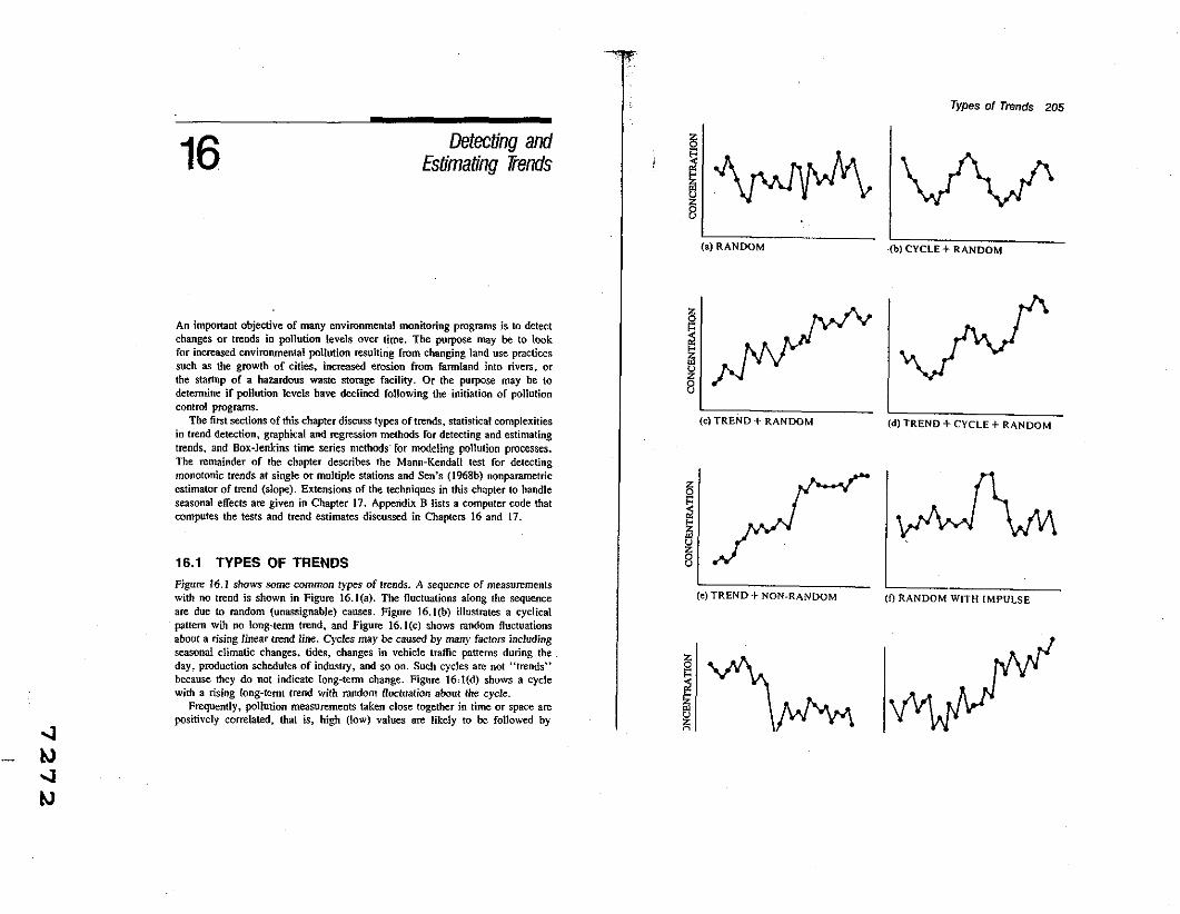
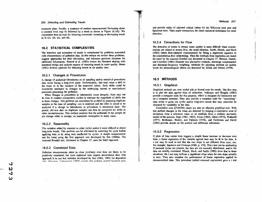
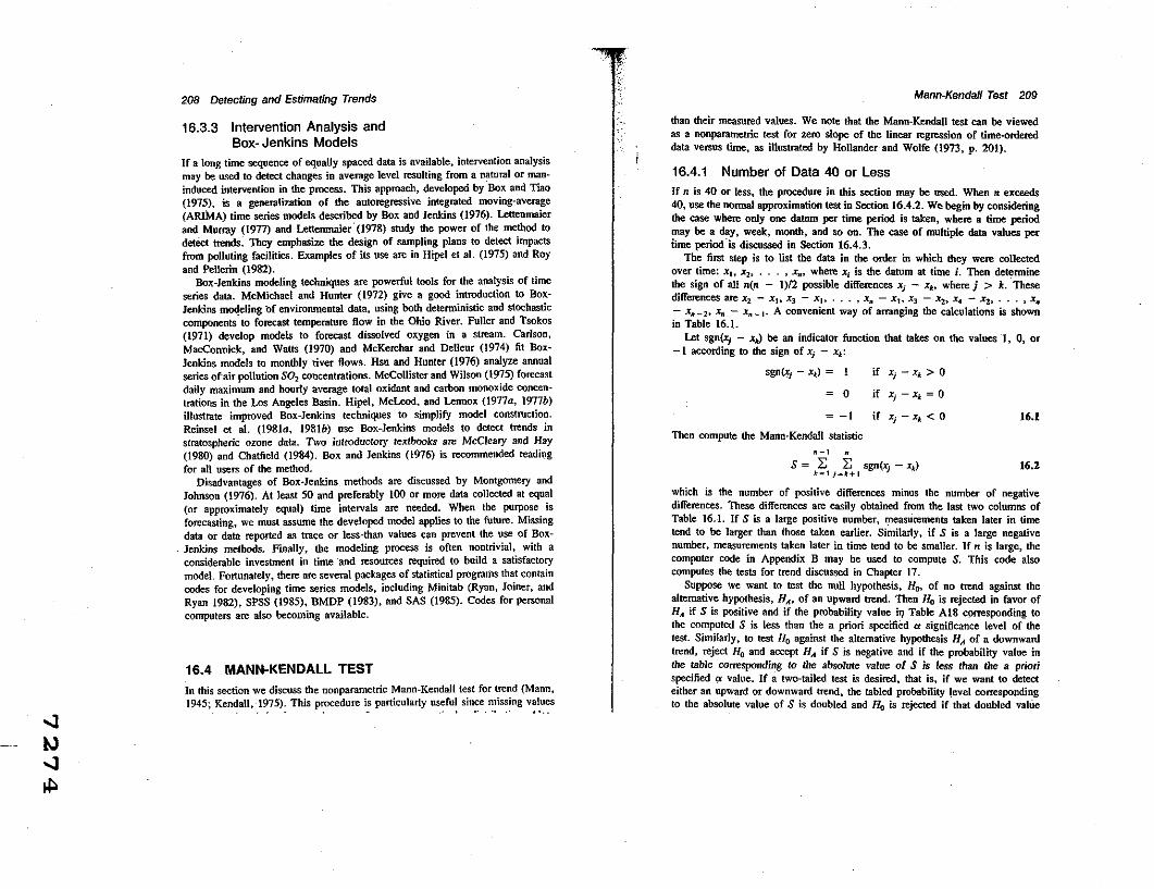
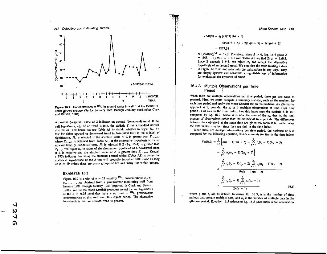
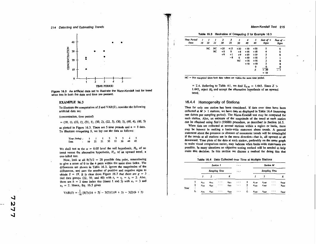
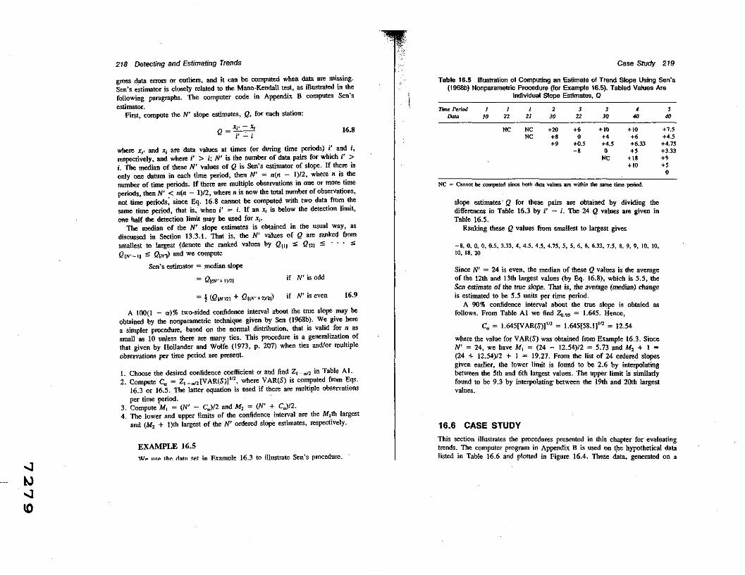
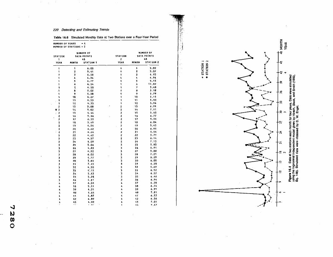
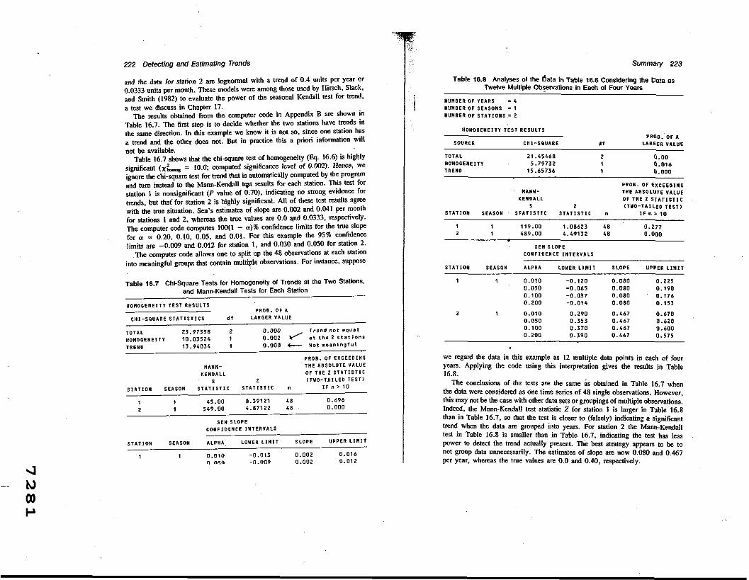
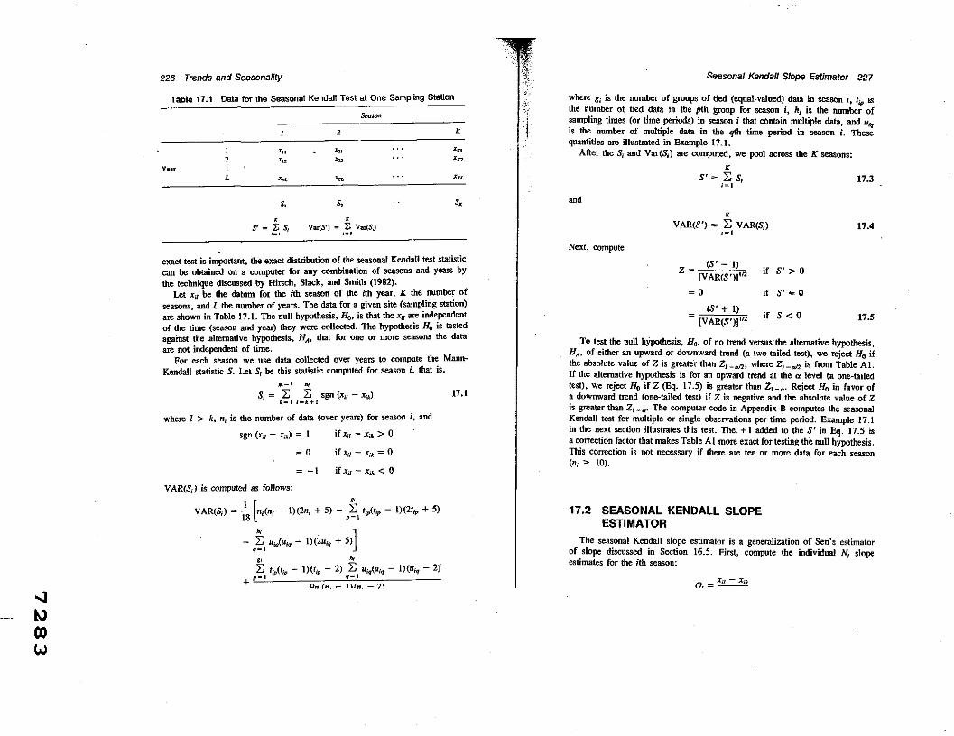
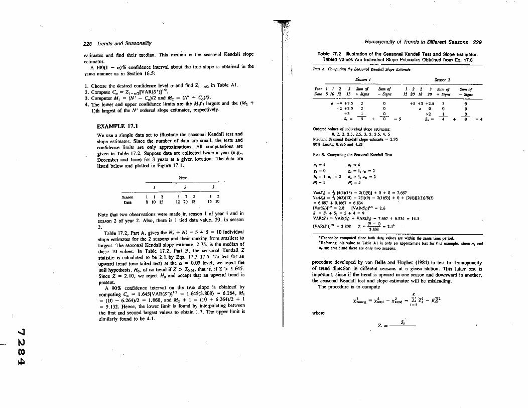
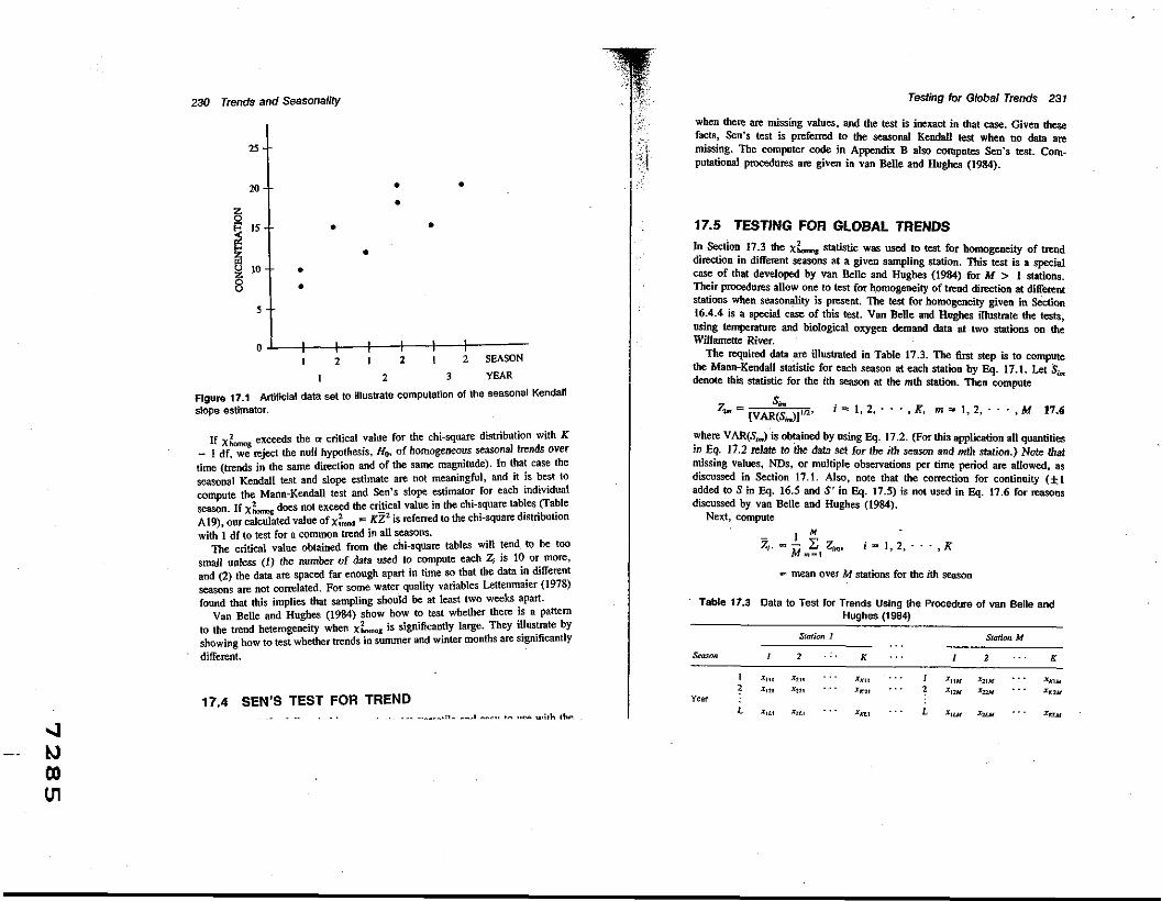
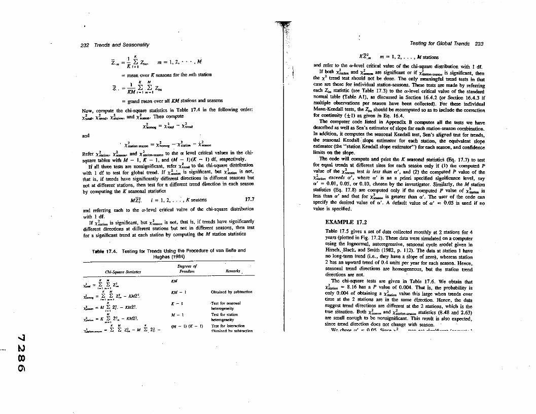
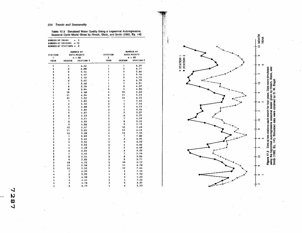
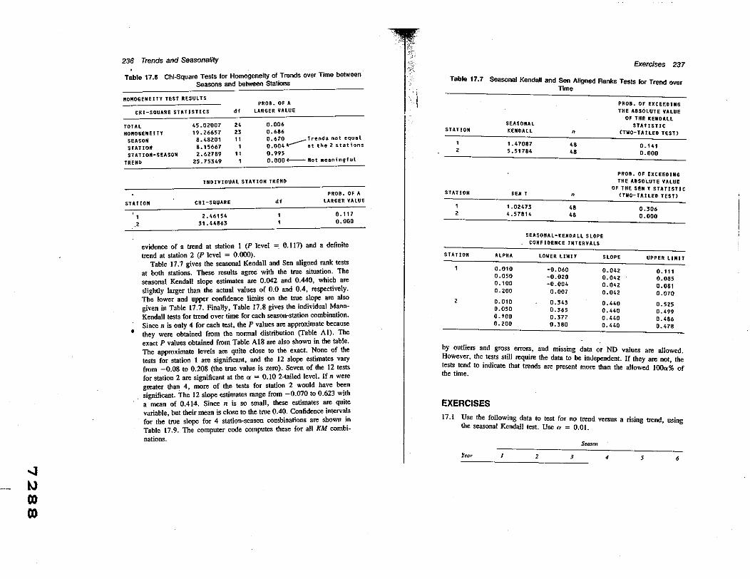
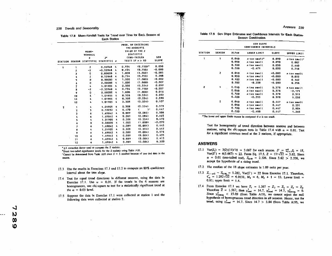Ddicarrdlo ~f~porenrsMa MargaretondDonoldIG i l k n

nilbwt is pinled on acid-Ire prpc 8 copyright0 1537 by John Wiley amp Sans Ins Allrights rewnnd

Pvblirhcd simuluncoudy in Canada

~ o p m a f t h i publication may beampaccd s u r d in smricval sysnm or tnnrmittd in any farma by any mcanrclce~oni mechanical pho~oeapyingmording scanttina w Mhawirc c i q t a s p r m i n d undnScelions I01 or 108 ofthe 1916 United Slaw CopyrightAct wilhml rirha ihr priorwrinenprmirion of ihc mbliahcr anuthonation amugh payment a1 thc

8ddruvdmUuPcrminionsDcpumunc John Wiley amp Smr 1ncW5 mid Avmuc New Y o 4 NY 10158M12 i212)850Mll lax (212) 8506m8 euro-Mail M-QWL~SYCOM

approptiaapusopy fee bUu Cowight Cl-ncccentcr m RarnuoalDrivr hnnaM A 01923 (978) lmfax (977504144 R-u to thc Pvhlitha fap r m i u i m Lould be

G i l M Richard0 memods m

Bibliogsphy p Includcr index

sraci~rica~ mvimnmmral ponution monitoring

I~ollaion-~nvirnnrnsnlal anpulsStarirtisa1 ~

Contents

11 Types and Objectives of Envimnmental Pollution Studies I I 12 Statistical Design and Analysis Pmblems 1 2 13 Overview of the Design and Analysis Pmeess 1 3 14 Summary 1 4

2 Sampling Environmental Populations 1 5

2 L Sampling in Space and Time 1 5 22 Target and Sampled Populations 1 7 23 Representative Units 9

-24 Choosing a Sam~line Plan I In~ 25 variability and Enor in Envimnmental Studies 1 LO 26 Case Study 1 13 27 Summary 1 15

3 Environmental Sampling Design 1 17

31 lntmduction 1 17 32 Criteria for Chmsiag a Sampling Plan 1 17 33 Methods for Selecting Sampling LoCaliations and Times 1 19 34 Summary 1 24

4 Simple Random Sampling 1 26

41 Basic Comeper 1 26 42 Eslimating tbe Mean and Total Amount 1 27 43 Effect of Measurement E m n 30 44 Number of Measurements Independent Data 1 30 45 Number of Mcasu~ments Conelated Data 35 46 Estimating VarO 1 42 47 Summary 1 4 3

5 Stratifled Random Sampling 1 45 c -

Types of Trends 205















Methods 207



163 METHODS

















= - I if 1 - x k lt O






( xnw D o t ~

I I0

2 is

3 I4

4 20

hof + tip

No -t i ~ ~





1VAR(S) = -[(- 1)(2n + 5) - 5 t(t - 1)(21 + 5)] 163

18 p = ~




i i i 1 3 5 7 9 II 1 3 5 7 9 11 IMONTH

I 2 YEAR




- 6(5)(12 + 5) - 2(1)(4 + 5) - 2(1)(4 + 511 f

= 122733








2 I (I - l)(lp - 2) 5 Juq - I)( - 2) P - I 9- I

+ 9n(rt - l)(n - 2)


+ 2( - 1)

165


C




i r l o 22 21 30 22 30 40 40 Sw S i p s

NC NC +20 +12 +20 +M +30 5 0 NC +8 0 + 8 +I8 +I8 4 0

+9 +I + 9 +19 +I9 5 0 --8 0 +lo +lo 2 I

NC +I8 +I8 2 0 f 10 +I0 2 0

0 - -0 S = m - I

= 19


I 2 3 4 5













1 2 K I 2 K







z = 4 167 ( ~ A R ( s ~ ) I ~





EXAivWLE 164




VAR(S) = 5(4)(15)-= 16667 and VAR(S2I8


Z=-- 7 -3 (166673~n- and amp = o= -0783

Thus

x2- = 171 + (-0783) - 2 (171 0783) = 31










S




= 4 ( Q ~ ~ ~ if ~N is even 169+ Q ~ ~ + ~ ~ )







Case Study 219



NC NC +20 +6 +I0 110 t75 NC +8 0 +d +6 +45

+9 +05 fd5 +633 i475 -8 0 +5 C333

NC +I8 +9 +to +5

0






C = 1645[VAR(S)] = 1645[58IJ1 = 1254







1 1 600 1 1 2 5 6 I 1 3 4 5 8 1 1 4 4 3 4 1 I 5 477 I




~~











I 1 4500 039121 L8 0696 2 1 54900 487122 48 0000



1 1 0010 -0013 0002 0016 n nm -0009 0002 0012

Summary 223
























amp







am

1 2 K

I XIS hl n

112 112 n

Yta 1 1 x x =rr







and

Next compute


- I










O - l gt f n - 7gt







sum 2 1 2 2 1 2 On 8 10 15 1220 18 1520












where


~(11I 2 1 2 1 2 S E A S O N

I 2 3 YEAR











Next compute




-

I = 2 X X - - 1 4 z I rnw 2 = 4 2 1 1r2 I X xx W

Year



- l XZ =-CZ r n = l 2 M

K t =













K m = l z MampampN






EXAMPLE 172



W = nnc 2 ---c- ~8







1 1 632 1 1 629 1 2 608 1 2 611 m C

1 3 516 1 3 566 -6 --0 ax-1 4 117 1 1 516 =E s0


--0 C -2 5 487 2 5 507 z 2 2 2 6 413 2 6 195 g 8 2 7 351 2 7 459 --2 5 z g2 8 132 2 8 522 m r r 2 9 106 2 9 513 2 10 147 2 10 569 2 11 505 2 11 641 2 12 520 2 12 753 3 1 583 3 1 702 3 2 565 3 2 693 3 3 532 3 3 655 m--

2223 1 533 3 4 666 3 5 420 3 5 669 -0 2 $8 3 6 385 3 6 523 N BG 3 7 145 3 7 511 lt E- - -c=

2= C =E45 -- rn





TOTAL 6502007 24 0006 80106EIElTY 1926657 23 0686

SEASON

SrArlON 818201 815667

11 1

0670 0001 J



TREND

262789 2575349

11 I



PROB OF A


1 246154 1 0117

2 3114863 1 0000





Exercises 237





1 147087 48 01412 551784 48 0000



1 102473 48 03062 157811 48 0000



1 0010 -0060 0042 0111 0050 0100 0200

-0020 -0004 0001

0042 0042 0042

0085 0081 0070


EXERCISES~ --







I 2 (TYO-rAlLED SEN


2 3 4

2 - 2

0 2

033968 -033968

000000 033968

4 1 4 4

0731 0731 1000 0731

(0750) (0750) (10001 107501

5 0 000000 4 1000 lt1000gt 6 8 9

10 1 1

0 4

-2 0 4 4

000000 101905

-03396 000000 101905 101905

4 4 4 4 1 6

1 ooo 0308 0731 1000 0308 0308

(1 000) (0334) (0750) (1000) (0334) (03341

1 2 1 101905 1 0308 (0334)

- -





Answers 239




-0171




0200 -0188 0147 1265



ANSWERS





Types of Trends 205















Methods 207



163 METHODS

















= - I if 1 - x k lt O






( xnw D o t ~

I I0

2 is

3 I4

4 20

hof + tip

No -t i ~ ~





1VAR(S) = -[(- 1)(2n + 5) - 5 t(t - 1)(21 + 5)] 163

18 p = ~




i i i 1 3 5 7 9 II 1 3 5 7 9 11 IMONTH

I 2 YEAR




- 6(5)(12 + 5) - 2(1)(4 + 5) - 2(1)(4 + 511 f

= 122733








2 I (I - l)(lp - 2) 5 Juq - I)( - 2) P - I 9- I

+ 9n(rt - l)(n - 2)


+ 2( - 1)

165


C




i r l o 22 21 30 22 30 40 40 Sw S i p s

NC NC +20 +12 +20 +M +30 5 0 NC +8 0 + 8 +I8 +I8 4 0

+9 +I + 9 +19 +I9 5 0 --8 0 +lo +lo 2 I

NC +I8 +I8 2 0 f 10 +I0 2 0

0 - -0 S = m - I

= 19


I 2 3 4 5













1 2 K I 2 K







z = 4 167 ( ~ A R ( s ~ ) I ~





EXAivWLE 164




VAR(S) = 5(4)(15)-= 16667 and VAR(S2I8


Z=-- 7 -3 (166673~n- and amp = o= -0783

Thus

x2- = 171 + (-0783) - 2 (171 0783) = 31










S




= 4 ( Q ~ ~ ~ if ~N is even 169+ Q ~ ~ + ~ ~ )







Case Study 219



NC NC +20 +6 +I0 110 t75 NC +8 0 +d +6 +45

+9 +05 fd5 +633 i475 -8 0 +5 C333

NC +I8 +9 +to +5

0






C = 1645[VAR(S)] = 1645[58IJ1 = 1254







1 1 600 1 1 2 5 6 I 1 3 4 5 8 1 1 4 4 3 4 1 I 5 477 I




~~











I 1 4500 039121 L8 0696 2 1 54900 487122 48 0000



1 1 0010 -0013 0002 0016 n nm -0009 0002 0012

Summary 223
























amp







am

1 2 K

I XIS hl n

112 112 n

Yta 1 1 x x =rr







and

Next compute


- I










O - l gt f n - 7gt







sum 2 1 2 2 1 2 On 8 10 15 1220 18 1520












where


~(11I 2 1 2 1 2 S E A S O N

I 2 3 YEAR











Next compute




-

I = 2 X X - - 1 4 z I rnw 2 = 4 2 1 1r2 I X xx W

Year



- l XZ =-CZ r n = l 2 M

K t =













K m = l z MampampN






EXAMPLE 172



W = nnc 2 ---c- ~8







1 1 632 1 1 629 1 2 608 1 2 611 m C

1 3 516 1 3 566 -6 --0 ax-1 4 117 1 1 516 =E s0


--0 C -2 5 487 2 5 507 z 2 2 2 6 413 2 6 195 g 8 2 7 351 2 7 459 --2 5 z g2 8 132 2 8 522 m r r 2 9 106 2 9 513 2 10 147 2 10 569 2 11 505 2 11 641 2 12 520 2 12 753 3 1 583 3 1 702 3 2 565 3 2 693 3 3 532 3 3 655 m--

2223 1 533 3 4 666 3 5 420 3 5 669 -0 2 $8 3 6 385 3 6 523 N BG 3 7 145 3 7 511 lt E- - -c=

2= C =E45 -- rn





TOTAL 6502007 24 0006 80106EIElTY 1926657 23 0686

SEASON

SrArlON 818201 815667

11 1

0670 0001 J



TREND

262789 2575349

11 I



PROB OF A


1 246154 1 0117

2 3114863 1 0000





Exercises 237





1 147087 48 01412 551784 48 0000



1 102473 48 03062 157811 48 0000



1 0010 -0060 0042 0111 0050 0100 0200

-0020 -0004 0001

0042 0042 0042

0085 0081 0070


EXERCISES~ --







I 2 (TYO-rAlLED SEN


2 3 4

2 - 2

0 2

033968 -033968

000000 033968

4 1 4 4

0731 0731 1000 0731

(0750) (0750) (10001 107501

5 0 000000 4 1000 lt1000gt 6 8 9

10 1 1

0 4

-2 0 4 4

000000 101905

-03396 000000 101905 101905

4 4 4 4 1 6

1 ooo 0308 0731 1000 0308 0308

(1 000) (0334) (0750) (1000) (0334) (03341

1 2 1 101905 1 0308 (0334)

- -





Answers 239




-0171




0200 -0188 0147 1265



ANSWERS












Methods 207



163 METHODS

















= - I if 1 - x k lt O






( xnw D o t ~

I I0

2 is

3 I4

4 20

hof + tip

No -t i ~ ~





1VAR(S) = -[(- 1)(2n + 5) - 5 t(t - 1)(21 + 5)] 163

18 p = ~




i i i 1 3 5 7 9 II 1 3 5 7 9 11 IMONTH

I 2 YEAR




- 6(5)(12 + 5) - 2(1)(4 + 5) - 2(1)(4 + 511 f

= 122733








2 I (I - l)(lp - 2) 5 Juq - I)( - 2) P - I 9- I

+ 9n(rt - l)(n - 2)


+ 2( - 1)

165


C




i r l o 22 21 30 22 30 40 40 Sw S i p s

NC NC +20 +12 +20 +M +30 5 0 NC +8 0 + 8 +I8 +I8 4 0

+9 +I + 9 +19 +I9 5 0 --8 0 +lo +lo 2 I

NC +I8 +I8 2 0 f 10 +I0 2 0

0 - -0 S = m - I

= 19


I 2 3 4 5













1 2 K I 2 K







z = 4 167 ( ~ A R ( s ~ ) I ~





EXAivWLE 164




VAR(S) = 5(4)(15)-= 16667 and VAR(S2I8


Z=-- 7 -3 (166673~n- and amp = o= -0783

Thus

x2- = 171 + (-0783) - 2 (171 0783) = 31










S




= 4 ( Q ~ ~ ~ if ~N is even 169+ Q ~ ~ + ~ ~ )







Case Study 219



NC NC +20 +6 +I0 110 t75 NC +8 0 +d +6 +45

+9 +05 fd5 +633 i475 -8 0 +5 C333

NC +I8 +9 +to +5

0






C = 1645[VAR(S)] = 1645[58IJ1 = 1254







1 1 600 1 1 2 5 6 I 1 3 4 5 8 1 1 4 4 3 4 1 I 5 477 I




~~











I 1 4500 039121 L8 0696 2 1 54900 487122 48 0000



1 1 0010 -0013 0002 0016 n nm -0009 0002 0012

Summary 223
























amp







am

1 2 K

I XIS hl n

112 112 n

Yta 1 1 x x =rr







and

Next compute


- I










O - l gt f n - 7gt







sum 2 1 2 2 1 2 On 8 10 15 1220 18 1520












where


~(11I 2 1 2 1 2 S E A S O N

I 2 3 YEAR











Next compute




-

I = 2 X X - - 1 4 z I rnw 2 = 4 2 1 1r2 I X xx W

Year



- l XZ =-CZ r n = l 2 M

K t =













K m = l z MampampN






EXAMPLE 172



W = nnc 2 ---c- ~8







1 1 632 1 1 629 1 2 608 1 2 611 m C

1 3 516 1 3 566 -6 --0 ax-1 4 117 1 1 516 =E s0


--0 C -2 5 487 2 5 507 z 2 2 2 6 413 2 6 195 g 8 2 7 351 2 7 459 --2 5 z g2 8 132 2 8 522 m r r 2 9 106 2 9 513 2 10 147 2 10 569 2 11 505 2 11 641 2 12 520 2 12 753 3 1 583 3 1 702 3 2 565 3 2 693 3 3 532 3 3 655 m--

2223 1 533 3 4 666 3 5 420 3 5 669 -0 2 $8 3 6 385 3 6 523 N BG 3 7 145 3 7 511 lt E- - -c=

2= C =E45 -- rn





TOTAL 6502007 24 0006 80106EIElTY 1926657 23 0686

SEASON

SrArlON 818201 815667

11 1

0670 0001 J



TREND

262789 2575349

11 I



PROB OF A


1 246154 1 0117

2 3114863 1 0000





Exercises 237





1 147087 48 01412 551784 48 0000



1 102473 48 03062 157811 48 0000



1 0010 -0060 0042 0111 0050 0100 0200

-0020 -0004 0001

0042 0042 0042

0085 0081 0070


EXERCISES~ --







I 2 (TYO-rAlLED SEN


2 3 4

2 - 2

0 2

033968 -033968

000000 033968

4 1 4 4

0731 0731 1000 0731

(0750) (0750) (10001 107501

5 0 000000 4 1000 lt1000gt 6 8 9

10 1 1

0 4

-2 0 4 4

000000 101905

-03396 000000 101905 101905

4 4 4 4 1 6

1 ooo 0308 0731 1000 0308 0308

(1 000) (0334) (0750) (1000) (0334) (03341

1 2 1 101905 1 0308 (0334)

- -





Answers 239




-0171




0200 -0188 0147 1265



ANSWERS


















= - I if 1 - x k lt O






( xnw D o t ~

I I0

2 is

3 I4

4 20

hof + tip

No -t i ~ ~





1VAR(S) = -[(- 1)(2n + 5) - 5 t(t - 1)(21 + 5)] 163

18 p = ~




i i i 1 3 5 7 9 II 1 3 5 7 9 11 IMONTH

I 2 YEAR




- 6(5)(12 + 5) - 2(1)(4 + 5) - 2(1)(4 + 511 f

= 122733








2 I (I - l)(lp - 2) 5 Juq - I)( - 2) P - I 9- I

+ 9n(rt - l)(n - 2)


+ 2( - 1)

165


C




i r l o 22 21 30 22 30 40 40 Sw S i p s

NC NC +20 +12 +20 +M +30 5 0 NC +8 0 + 8 +I8 +I8 4 0

+9 +I + 9 +19 +I9 5 0 --8 0 +lo +lo 2 I

NC +I8 +I8 2 0 f 10 +I0 2 0

0 - -0 S = m - I

= 19


I 2 3 4 5













1 2 K I 2 K







z = 4 167 ( ~ A R ( s ~ ) I ~





EXAivWLE 164




VAR(S) = 5(4)(15)-= 16667 and VAR(S2I8


Z=-- 7 -3 (166673~n- and amp = o= -0783

Thus

x2- = 171 + (-0783) - 2 (171 0783) = 31










S




= 4 ( Q ~ ~ ~ if ~N is even 169+ Q ~ ~ + ~ ~ )







Case Study 219



NC NC +20 +6 +I0 110 t75 NC +8 0 +d +6 +45

+9 +05 fd5 +633 i475 -8 0 +5 C333

NC +I8 +9 +to +5

0






C = 1645[VAR(S)] = 1645[58IJ1 = 1254







1 1 600 1 1 2 5 6 I 1 3 4 5 8 1 1 4 4 3 4 1 I 5 477 I




~~











I 1 4500 039121 L8 0696 2 1 54900 487122 48 0000



1 1 0010 -0013 0002 0016 n nm -0009 0002 0012

Summary 223
























amp







am

1 2 K

I XIS hl n

112 112 n

Yta 1 1 x x =rr







and

Next compute


- I










O - l gt f n - 7gt







sum 2 1 2 2 1 2 On 8 10 15 1220 18 1520












where


~(11I 2 1 2 1 2 S E A S O N

I 2 3 YEAR











Next compute




-

I = 2 X X - - 1 4 z I rnw 2 = 4 2 1 1r2 I X xx W

Year



- l XZ =-CZ r n = l 2 M

K t =













K m = l z MampampN






EXAMPLE 172



W = nnc 2 ---c- ~8







1 1 632 1 1 629 1 2 608 1 2 611 m C

1 3 516 1 3 566 -6 --0 ax-1 4 117 1 1 516 =E s0


--0 C -2 5 487 2 5 507 z 2 2 2 6 413 2 6 195 g 8 2 7 351 2 7 459 --2 5 z g2 8 132 2 8 522 m r r 2 9 106 2 9 513 2 10 147 2 10 569 2 11 505 2 11 641 2 12 520 2 12 753 3 1 583 3 1 702 3 2 565 3 2 693 3 3 532 3 3 655 m--

2223 1 533 3 4 666 3 5 420 3 5 669 -0 2 $8 3 6 385 3 6 523 N BG 3 7 145 3 7 511 lt E- - -c=

2= C =E45 -- rn





TOTAL 6502007 24 0006 80106EIElTY 1926657 23 0686

SEASON

SrArlON 818201 815667

11 1

0670 0001 J



TREND

262789 2575349

11 I



PROB OF A


1 246154 1 0117

2 3114863 1 0000





Exercises 237





1 147087 48 01412 551784 48 0000



1 102473 48 03062 157811 48 0000



1 0010 -0060 0042 0111 0050 0100 0200

-0020 -0004 0001

0042 0042 0042

0085 0081 0070


EXERCISES~ --







I 2 (TYO-rAlLED SEN


2 3 4

2 - 2

0 2

033968 -033968

000000 033968

4 1 4 4

0731 0731 1000 0731

(0750) (0750) (10001 107501

5 0 000000 4 1000 lt1000gt 6 8 9

10 1 1

0 4

-2 0 4 4

000000 101905

-03396 000000 101905 101905

4 4 4 4 1 6

1 ooo 0308 0731 1000 0308 0308

(1 000) (0334) (0750) (1000) (0334) (03341

1 2 1 101905 1 0308 (0334)

- -





Answers 239




-0171




0200 -0188 0147 1265



ANSWERS







( xnw D o t ~

I I0

2 is

3 I4

4 20

hof + tip

No -t i ~ ~





1VAR(S) = -[(- 1)(2n + 5) - 5 t(t - 1)(21 + 5)] 163

18 p = ~




i i i 1 3 5 7 9 II 1 3 5 7 9 11 IMONTH

I 2 YEAR




- 6(5)(12 + 5) - 2(1)(4 + 5) - 2(1)(4 + 511 f

= 122733








2 I (I - l)(lp - 2) 5 Juq - I)( - 2) P - I 9- I

+ 9n(rt - l)(n - 2)


+ 2( - 1)

165


C




i r l o 22 21 30 22 30 40 40 Sw S i p s

NC NC +20 +12 +20 +M +30 5 0 NC +8 0 + 8 +I8 +I8 4 0

+9 +I + 9 +19 +I9 5 0 --8 0 +lo +lo 2 I

NC +I8 +I8 2 0 f 10 +I0 2 0

0 - -0 S = m - I

= 19


I 2 3 4 5













1 2 K I 2 K







z = 4 167 ( ~ A R ( s ~ ) I ~





EXAivWLE 164




VAR(S) = 5(4)(15)-= 16667 and VAR(S2I8


Z=-- 7 -3 (166673~n- and amp = o= -0783

Thus

x2- = 171 + (-0783) - 2 (171 0783) = 31










S




= 4 ( Q ~ ~ ~ if ~N is even 169+ Q ~ ~ + ~ ~ )







Case Study 219



NC NC +20 +6 +I0 110 t75 NC +8 0 +d +6 +45

+9 +05 fd5 +633 i475 -8 0 +5 C333

NC +I8 +9 +to +5

0






C = 1645[VAR(S)] = 1645[58IJ1 = 1254







1 1 600 1 1 2 5 6 I 1 3 4 5 8 1 1 4 4 3 4 1 I 5 477 I




~~











I 1 4500 039121 L8 0696 2 1 54900 487122 48 0000



1 1 0010 -0013 0002 0016 n nm -0009 0002 0012

Summary 223
























amp







am

1 2 K

I XIS hl n

112 112 n

Yta 1 1 x x =rr







and

Next compute


- I










O - l gt f n - 7gt







sum 2 1 2 2 1 2 On 8 10 15 1220 18 1520












where


~(11I 2 1 2 1 2 S E A S O N

I 2 3 YEAR











Next compute




-

I = 2 X X - - 1 4 z I rnw 2 = 4 2 1 1r2 I X xx W

Year



- l XZ =-CZ r n = l 2 M

K t =













K m = l z MampampN






EXAMPLE 172



W = nnc 2 ---c- ~8







1 1 632 1 1 629 1 2 608 1 2 611 m C

1 3 516 1 3 566 -6 --0 ax-1 4 117 1 1 516 =E s0


--0 C -2 5 487 2 5 507 z 2 2 2 6 413 2 6 195 g 8 2 7 351 2 7 459 --2 5 z g2 8 132 2 8 522 m r r 2 9 106 2 9 513 2 10 147 2 10 569 2 11 505 2 11 641 2 12 520 2 12 753 3 1 583 3 1 702 3 2 565 3 2 693 3 3 532 3 3 655 m--

2223 1 533 3 4 666 3 5 420 3 5 669 -0 2 $8 3 6 385 3 6 523 N BG 3 7 145 3 7 511 lt E- - -c=

2= C =E45 -- rn





TOTAL 6502007 24 0006 80106EIElTY 1926657 23 0686

SEASON

SrArlON 818201 815667

11 1

0670 0001 J



TREND

262789 2575349

11 I



PROB OF A


1 246154 1 0117

2 3114863 1 0000





Exercises 237





1 147087 48 01412 551784 48 0000



1 102473 48 03062 157811 48 0000



1 0010 -0060 0042 0111 0050 0100 0200

-0020 -0004 0001

0042 0042 0042

0085 0081 0070


EXERCISES~ --







I 2 (TYO-rAlLED SEN


2 3 4

2 - 2

0 2

033968 -033968

000000 033968

4 1 4 4

0731 0731 1000 0731

(0750) (0750) (10001 107501

5 0 000000 4 1000 lt1000gt 6 8 9

10 1 1

0 4

-2 0 4 4

000000 101905

-03396 000000 101905 101905

4 4 4 4 1 6

1 ooo 0308 0731 1000 0308 0308

(1 000) (0334) (0750) (1000) (0334) (03341

1 2 1 101905 1 0308 (0334)

- -





Answers 239




-0171




0200 -0188 0147 1265



ANSWERS






i i i 1 3 5 7 9 II 1 3 5 7 9 11 IMONTH

I 2 YEAR




- 6(5)(12 + 5) - 2(1)(4 + 5) - 2(1)(4 + 511 f

= 122733








2 I (I - l)(lp - 2) 5 Juq - I)( - 2) P - I 9- I

+ 9n(rt - l)(n - 2)


+ 2( - 1)

165


C




i r l o 22 21 30 22 30 40 40 Sw S i p s

NC NC +20 +12 +20 +M +30 5 0 NC +8 0 + 8 +I8 +I8 4 0

+9 +I + 9 +19 +I9 5 0 --8 0 +lo +lo 2 I

NC +I8 +I8 2 0 f 10 +I0 2 0

0 - -0 S = m - I

= 19


I 2 3 4 5













1 2 K I 2 K







z = 4 167 ( ~ A R ( s ~ ) I ~





EXAivWLE 164




VAR(S) = 5(4)(15)-= 16667 and VAR(S2I8


Z=-- 7 -3 (166673~n- and amp = o= -0783

Thus

x2- = 171 + (-0783) - 2 (171 0783) = 31










S




= 4 ( Q ~ ~ ~ if ~N is even 169+ Q ~ ~ + ~ ~ )







Case Study 219



NC NC +20 +6 +I0 110 t75 NC +8 0 +d +6 +45

+9 +05 fd5 +633 i475 -8 0 +5 C333

NC +I8 +9 +to +5

0






C = 1645[VAR(S)] = 1645[58IJ1 = 1254







1 1 600 1 1 2 5 6 I 1 3 4 5 8 1 1 4 4 3 4 1 I 5 477 I




~~











I 1 4500 039121 L8 0696 2 1 54900 487122 48 0000



1 1 0010 -0013 0002 0016 n nm -0009 0002 0012

Summary 223
























amp







am

1 2 K

I XIS hl n

112 112 n

Yta 1 1 x x =rr







and

Next compute


- I










O - l gt f n - 7gt







sum 2 1 2 2 1 2 On 8 10 15 1220 18 1520












where


~(11I 2 1 2 1 2 S E A S O N

I 2 3 YEAR











Next compute




-

I = 2 X X - - 1 4 z I rnw 2 = 4 2 1 1r2 I X xx W

Year



- l XZ =-CZ r n = l 2 M

K t =













K m = l z MampampN






EXAMPLE 172



W = nnc 2 ---c- ~8







1 1 632 1 1 629 1 2 608 1 2 611 m C

1 3 516 1 3 566 -6 --0 ax-1 4 117 1 1 516 =E s0


--0 C -2 5 487 2 5 507 z 2 2 2 6 413 2 6 195 g 8 2 7 351 2 7 459 --2 5 z g2 8 132 2 8 522 m r r 2 9 106 2 9 513 2 10 147 2 10 569 2 11 505 2 11 641 2 12 520 2 12 753 3 1 583 3 1 702 3 2 565 3 2 693 3 3 532 3 3 655 m--

2223 1 533 3 4 666 3 5 420 3 5 669 -0 2 $8 3 6 385 3 6 523 N BG 3 7 145 3 7 511 lt E- - -c=

2= C =E45 -- rn





TOTAL 6502007 24 0006 80106EIElTY 1926657 23 0686

SEASON

SrArlON 818201 815667

11 1

0670 0001 J



TREND

262789 2575349

11 I



PROB OF A


1 246154 1 0117

2 3114863 1 0000





Exercises 237





1 147087 48 01412 551784 48 0000



1 102473 48 03062 157811 48 0000



1 0010 -0060 0042 0111 0050 0100 0200

-0020 -0004 0001

0042 0042 0042

0085 0081 0070


EXERCISES~ --







I 2 (TYO-rAlLED SEN


2 3 4

2 - 2

0 2

033968 -033968

000000 033968

4 1 4 4

0731 0731 1000 0731

(0750) (0750) (10001 107501

5 0 000000 4 1000 lt1000gt 6 8 9

10 1 1

0 4

-2 0 4 4

000000 101905

-03396 000000 101905 101905

4 4 4 4 1 6

1 ooo 0308 0731 1000 0308 0308

(1 000) (0334) (0750) (1000) (0334) (03341

1 2 1 101905 1 0308 (0334)

- -





Answers 239




-0171




0200 -0188 0147 1265



ANSWERS





C




i r l o 22 21 30 22 30 40 40 Sw S i p s

NC NC +20 +12 +20 +M +30 5 0 NC +8 0 + 8 +I8 +I8 4 0

+9 +I + 9 +19 +I9 5 0 --8 0 +lo +lo 2 I

NC +I8 +I8 2 0 f 10 +I0 2 0

0 - -0 S = m - I

= 19


I 2 3 4 5













1 2 K I 2 K







z = 4 167 ( ~ A R ( s ~ ) I ~





EXAivWLE 164




VAR(S) = 5(4)(15)-= 16667 and VAR(S2I8


Z=-- 7 -3 (166673~n- and amp = o= -0783

Thus

x2- = 171 + (-0783) - 2 (171 0783) = 31










S




= 4 ( Q ~ ~ ~ if ~N is even 169+ Q ~ ~ + ~ ~ )







Case Study 219



NC NC +20 +6 +I0 110 t75 NC +8 0 +d +6 +45

+9 +05 fd5 +633 i475 -8 0 +5 C333

NC +I8 +9 +to +5

0






C = 1645[VAR(S)] = 1645[58IJ1 = 1254







1 1 600 1 1 2 5 6 I 1 3 4 5 8 1 1 4 4 3 4 1 I 5 477 I




~~











I 1 4500 039121 L8 0696 2 1 54900 487122 48 0000



1 1 0010 -0013 0002 0016 n nm -0009 0002 0012

Summary 223
























amp







am

1 2 K

I XIS hl n

112 112 n

Yta 1 1 x x =rr







and

Next compute


- I










O - l gt f n - 7gt







sum 2 1 2 2 1 2 On 8 10 15 1220 18 1520












where


~(11I 2 1 2 1 2 S E A S O N

I 2 3 YEAR











Next compute




-

I = 2 X X - - 1 4 z I rnw 2 = 4 2 1 1r2 I X xx W

Year



- l XZ =-CZ r n = l 2 M

K t =













K m = l z MampampN






EXAMPLE 172



W = nnc 2 ---c- ~8







1 1 632 1 1 629 1 2 608 1 2 611 m C

1 3 516 1 3 566 -6 --0 ax-1 4 117 1 1 516 =E s0


--0 C -2 5 487 2 5 507 z 2 2 2 6 413 2 6 195 g 8 2 7 351 2 7 459 --2 5 z g2 8 132 2 8 522 m r r 2 9 106 2 9 513 2 10 147 2 10 569 2 11 505 2 11 641 2 12 520 2 12 753 3 1 583 3 1 702 3 2 565 3 2 693 3 3 532 3 3 655 m--

2223 1 533 3 4 666 3 5 420 3 5 669 -0 2 $8 3 6 385 3 6 523 N BG 3 7 145 3 7 511 lt E- - -c=

2= C =E45 -- rn





TOTAL 6502007 24 0006 80106EIElTY 1926657 23 0686

SEASON

SrArlON 818201 815667

11 1

0670 0001 J



TREND

262789 2575349

11 I



PROB OF A


1 246154 1 0117

2 3114863 1 0000





Exercises 237





1 147087 48 01412 551784 48 0000



1 102473 48 03062 157811 48 0000



1 0010 -0060 0042 0111 0050 0100 0200

-0020 -0004 0001

0042 0042 0042

0085 0081 0070


EXERCISES~ --







I 2 (TYO-rAlLED SEN


2 3 4

2 - 2

0 2

033968 -033968

000000 033968

4 1 4 4

0731 0731 1000 0731

(0750) (0750) (10001 107501

5 0 000000 4 1000 lt1000gt 6 8 9

10 1 1

0 4

-2 0 4 4

000000 101905

-03396 000000 101905 101905

4 4 4 4 1 6

1 ooo 0308 0731 1000 0308 0308

(1 000) (0334) (0750) (1000) (0334) (03341

1 2 1 101905 1 0308 (0334)

- -





Answers 239




-0171




0200 -0188 0147 1265



ANSWERS








z = 4 167 ( ~ A R ( s ~ ) I ~





EXAivWLE 164




VAR(S) = 5(4)(15)-= 16667 and VAR(S2I8


Z=-- 7 -3 (166673~n- and amp = o= -0783

Thus

x2- = 171 + (-0783) - 2 (171 0783) = 31










S




= 4 ( Q ~ ~ ~ if ~N is even 169+ Q ~ ~ + ~ ~ )







Case Study 219



NC NC +20 +6 +I0 110 t75 NC +8 0 +d +6 +45

+9 +05 fd5 +633 i475 -8 0 +5 C333

NC +I8 +9 +to +5

0






C = 1645[VAR(S)] = 1645[58IJ1 = 1254







1 1 600 1 1 2 5 6 I 1 3 4 5 8 1 1 4 4 3 4 1 I 5 477 I




~~











I 1 4500 039121 L8 0696 2 1 54900 487122 48 0000



1 1 0010 -0013 0002 0016 n nm -0009 0002 0012

Summary 223
























amp







am

1 2 K

I XIS hl n

112 112 n

Yta 1 1 x x =rr







and

Next compute


- I










O - l gt f n - 7gt







sum 2 1 2 2 1 2 On 8 10 15 1220 18 1520












where


~(11I 2 1 2 1 2 S E A S O N

I 2 3 YEAR











Next compute




-

I = 2 X X - - 1 4 z I rnw 2 = 4 2 1 1r2 I X xx W

Year



- l XZ =-CZ r n = l 2 M

K t =













K m = l z MampampN






EXAMPLE 172



W = nnc 2 ---c- ~8







1 1 632 1 1 629 1 2 608 1 2 611 m C

1 3 516 1 3 566 -6 --0 ax-1 4 117 1 1 516 =E s0


--0 C -2 5 487 2 5 507 z 2 2 2 6 413 2 6 195 g 8 2 7 351 2 7 459 --2 5 z g2 8 132 2 8 522 m r r 2 9 106 2 9 513 2 10 147 2 10 569 2 11 505 2 11 641 2 12 520 2 12 753 3 1 583 3 1 702 3 2 565 3 2 693 3 3 532 3 3 655 m--

2223 1 533 3 4 666 3 5 420 3 5 669 -0 2 $8 3 6 385 3 6 523 N BG 3 7 145 3 7 511 lt E- - -c=

2= C =E45 -- rn





TOTAL 6502007 24 0006 80106EIElTY 1926657 23 0686

SEASON

SrArlON 818201 815667

11 1

0670 0001 J



TREND

262789 2575349

11 I



PROB OF A


1 246154 1 0117

2 3114863 1 0000





Exercises 237





1 147087 48 01412 551784 48 0000



1 102473 48 03062 157811 48 0000



1 0010 -0060 0042 0111 0050 0100 0200

-0020 -0004 0001

0042 0042 0042

0085 0081 0070


EXERCISES~ --







I 2 (TYO-rAlLED SEN


2 3 4

2 - 2

0 2

033968 -033968

000000 033968

4 1 4 4

0731 0731 1000 0731

(0750) (0750) (10001 107501

5 0 000000 4 1000 lt1000gt 6 8 9

10 1 1

0 4

-2 0 4 4

000000 101905

-03396 000000 101905 101905

4 4 4 4 1 6

1 ooo 0308 0731 1000 0308 0308

(1 000) (0334) (0750) (1000) (0334) (03341

1 2 1 101905 1 0308 (0334)

- -





Answers 239




-0171




0200 -0188 0147 1265



ANSWERS










S




= 4 ( Q ~ ~ ~ if ~N is even 169+ Q ~ ~ + ~ ~ )







Case Study 219



NC NC +20 +6 +I0 110 t75 NC +8 0 +d +6 +45

+9 +05 fd5 +633 i475 -8 0 +5 C333

NC +I8 +9 +to +5

0






C = 1645[VAR(S)] = 1645[58IJ1 = 1254







1 1 600 1 1 2 5 6 I 1 3 4 5 8 1 1 4 4 3 4 1 I 5 477 I




~~











I 1 4500 039121 L8 0696 2 1 54900 487122 48 0000



1 1 0010 -0013 0002 0016 n nm -0009 0002 0012

Summary 223
























amp







am

1 2 K

I XIS hl n

112 112 n

Yta 1 1 x x =rr







and

Next compute


- I










O - l gt f n - 7gt







sum 2 1 2 2 1 2 On 8 10 15 1220 18 1520












where


~(11I 2 1 2 1 2 S E A S O N

I 2 3 YEAR











Next compute




-

I = 2 X X - - 1 4 z I rnw 2 = 4 2 1 1r2 I X xx W

Year



- l XZ =-CZ r n = l 2 M

K t =













K m = l z MampampN






EXAMPLE 172



W = nnc 2 ---c- ~8







1 1 632 1 1 629 1 2 608 1 2 611 m C

1 3 516 1 3 566 -6 --0 ax-1 4 117 1 1 516 =E s0


--0 C -2 5 487 2 5 507 z 2 2 2 6 413 2 6 195 g 8 2 7 351 2 7 459 --2 5 z g2 8 132 2 8 522 m r r 2 9 106 2 9 513 2 10 147 2 10 569 2 11 505 2 11 641 2 12 520 2 12 753 3 1 583 3 1 702 3 2 565 3 2 693 3 3 532 3 3 655 m--

2223 1 533 3 4 666 3 5 420 3 5 669 -0 2 $8 3 6 385 3 6 523 N BG 3 7 145 3 7 511 lt E- - -c=

2= C =E45 -- rn





TOTAL 6502007 24 0006 80106EIElTY 1926657 23 0686

SEASON

SrArlON 818201 815667

11 1

0670 0001 J



TREND

262789 2575349

11 I



PROB OF A


1 246154 1 0117

2 3114863 1 0000





Exercises 237





1 147087 48 01412 551784 48 0000



1 102473 48 03062 157811 48 0000



1 0010 -0060 0042 0111 0050 0100 0200

-0020 -0004 0001

0042 0042 0042

0085 0081 0070


EXERCISES~ --







I 2 (TYO-rAlLED SEN


2 3 4

2 - 2

0 2

033968 -033968

000000 033968

4 1 4 4

0731 0731 1000 0731

(0750) (0750) (10001 107501

5 0 000000 4 1000 lt1000gt 6 8 9

10 1 1

0 4

-2 0 4 4

000000 101905

-03396 000000 101905 101905

4 4 4 4 1 6

1 ooo 0308 0731 1000 0308 0308

(1 000) (0334) (0750) (1000) (0334) (03341

1 2 1 101905 1 0308 (0334)

- -





Answers 239




-0171




0200 -0188 0147 1265



ANSWERS









1 1 600 1 1 2 5 6 I 1 3 4 5 8 1 1 4 4 3 4 1 I 5 477 I




~~











I 1 4500 039121 L8 0696 2 1 54900 487122 48 0000



1 1 0010 -0013 0002 0016 n nm -0009 0002 0012

Summary 223
























amp







am

1 2 K

I XIS hl n

112 112 n

Yta 1 1 x x =rr







and

Next compute


- I










O - l gt f n - 7gt







sum 2 1 2 2 1 2 On 8 10 15 1220 18 1520












where


~(11I 2 1 2 1 2 S E A S O N

I 2 3 YEAR











Next compute




-

I = 2 X X - - 1 4 z I rnw 2 = 4 2 1 1r2 I X xx W

Year



- l XZ =-CZ r n = l 2 M

K t =













K m = l z MampampN






EXAMPLE 172



W = nnc 2 ---c- ~8







1 1 632 1 1 629 1 2 608 1 2 611 m C

1 3 516 1 3 566 -6 --0 ax-1 4 117 1 1 516 =E s0


--0 C -2 5 487 2 5 507 z 2 2 2 6 413 2 6 195 g 8 2 7 351 2 7 459 --2 5 z g2 8 132 2 8 522 m r r 2 9 106 2 9 513 2 10 147 2 10 569 2 11 505 2 11 641 2 12 520 2 12 753 3 1 583 3 1 702 3 2 565 3 2 693 3 3 532 3 3 655 m--

2223 1 533 3 4 666 3 5 420 3 5 669 -0 2 $8 3 6 385 3 6 523 N BG 3 7 145 3 7 511 lt E- - -c=

2= C =E45 -- rn





TOTAL 6502007 24 0006 80106EIElTY 1926657 23 0686

SEASON

SrArlON 818201 815667

11 1

0670 0001 J



TREND

262789 2575349

11 I



PROB OF A


1 246154 1 0117

2 3114863 1 0000





Exercises 237





1 147087 48 01412 551784 48 0000



1 102473 48 03062 157811 48 0000



1 0010 -0060 0042 0111 0050 0100 0200

-0020 -0004 0001

0042 0042 0042

0085 0081 0070


EXERCISES~ --







I 2 (TYO-rAlLED SEN


2 3 4

2 - 2

0 2

033968 -033968

000000 033968

4 1 4 4

0731 0731 1000 0731

(0750) (0750) (10001 107501

5 0 000000 4 1000 lt1000gt 6 8 9

10 1 1

0 4

-2 0 4 4

000000 101905

-03396 000000 101905 101905

4 4 4 4 1 6

1 ooo 0308 0731 1000 0308 0308

(1 000) (0334) (0750) (1000) (0334) (03341

1 2 1 101905 1 0308 (0334)

- -





Answers 239




-0171




0200 -0188 0147 1265



ANSWERS








~~











I 1 4500 039121 L8 0696 2 1 54900 487122 48 0000



1 1 0010 -0013 0002 0016 n nm -0009 0002 0012

Summary 223
























amp







am

1 2 K

I XIS hl n

112 112 n

Yta 1 1 x x =rr







and

Next compute


- I










O - l gt f n - 7gt







sum 2 1 2 2 1 2 On 8 10 15 1220 18 1520












where


~(11I 2 1 2 1 2 S E A S O N

I 2 3 YEAR











Next compute




-

I = 2 X X - - 1 4 z I rnw 2 = 4 2 1 1r2 I X xx W

Year



- l XZ =-CZ r n = l 2 M

K t =













K m = l z MampampN






EXAMPLE 172



W = nnc 2 ---c- ~8







1 1 632 1 1 629 1 2 608 1 2 611 m C

1 3 516 1 3 566 -6 --0 ax-1 4 117 1 1 516 =E s0


--0 C -2 5 487 2 5 507 z 2 2 2 6 413 2 6 195 g 8 2 7 351 2 7 459 --2 5 z g2 8 132 2 8 522 m r r 2 9 106 2 9 513 2 10 147 2 10 569 2 11 505 2 11 641 2 12 520 2 12 753 3 1 583 3 1 702 3 2 565 3 2 693 3 3 532 3 3 655 m--

2223 1 533 3 4 666 3 5 420 3 5 669 -0 2 $8 3 6 385 3 6 523 N BG 3 7 145 3 7 511 lt E- - -c=

2= C =E45 -- rn





TOTAL 6502007 24 0006 80106EIElTY 1926657 23 0686

SEASON

SrArlON 818201 815667

11 1

0670 0001 J



TREND

262789 2575349

11 I



PROB OF A


1 246154 1 0117

2 3114863 1 0000





Exercises 237





1 147087 48 01412 551784 48 0000



1 102473 48 03062 157811 48 0000



1 0010 -0060 0042 0111 0050 0100 0200

-0020 -0004 0001

0042 0042 0042

0085 0081 0070


EXERCISES~ --







I 2 (TYO-rAlLED SEN


2 3 4

2 - 2

0 2

033968 -033968

000000 033968

4 1 4 4

0731 0731 1000 0731

(0750) (0750) (10001 107501

5 0 000000 4 1000 lt1000gt 6 8 9

10 1 1

0 4

-2 0 4 4

000000 101905

-03396 000000 101905 101905

4 4 4 4 1 6

1 ooo 0308 0731 1000 0308 0308

(1 000) (0334) (0750) (1000) (0334) (03341

1 2 1 101905 1 0308 (0334)

- -





Answers 239




-0171




0200 -0188 0147 1265



ANSWERS

















amp







am

1 2 K

I XIS hl n

112 112 n

Yta 1 1 x x =rr







and

Next compute


- I










O - l gt f n - 7gt







sum 2 1 2 2 1 2 On 8 10 15 1220 18 1520












where


~(11I 2 1 2 1 2 S E A S O N

I 2 3 YEAR











Next compute




-

I = 2 X X - - 1 4 z I rnw 2 = 4 2 1 1r2 I X xx W

Year



- l XZ =-CZ r n = l 2 M

K t =













K m = l z MampampN






EXAMPLE 172



W = nnc 2 ---c- ~8







1 1 632 1 1 629 1 2 608 1 2 611 m C

1 3 516 1 3 566 -6 --0 ax-1 4 117 1 1 516 =E s0


--0 C -2 5 487 2 5 507 z 2 2 2 6 413 2 6 195 g 8 2 7 351 2 7 459 --2 5 z g2 8 132 2 8 522 m r r 2 9 106 2 9 513 2 10 147 2 10 569 2 11 505 2 11 641 2 12 520 2 12 753 3 1 583 3 1 702 3 2 565 3 2 693 3 3 532 3 3 655 m--

2223 1 533 3 4 666 3 5 420 3 5 669 -0 2 $8 3 6 385 3 6 523 N BG 3 7 145 3 7 511 lt E- - -c=

2= C =E45 -- rn





TOTAL 6502007 24 0006 80106EIElTY 1926657 23 0686

SEASON

SrArlON 818201 815667

11 1

0670 0001 J



TREND

262789 2575349

11 I



PROB OF A


1 246154 1 0117

2 3114863 1 0000





Exercises 237





1 147087 48 01412 551784 48 0000



1 102473 48 03062 157811 48 0000



1 0010 -0060 0042 0111 0050 0100 0200

-0020 -0004 0001

0042 0042 0042

0085 0081 0070


EXERCISES~ --







I 2 (TYO-rAlLED SEN


2 3 4

2 - 2

0 2

033968 -033968

000000 033968

4 1 4 4

0731 0731 1000 0731

(0750) (0750) (10001 107501

5 0 000000 4 1000 lt1000gt 6 8 9

10 1 1

0 4

-2 0 4 4

000000 101905

-03396 000000 101905 101905

4 4 4 4 1 6

1 ooo 0308 0731 1000 0308 0308

(1 000) (0334) (0750) (1000) (0334) (03341

1 2 1 101905 1 0308 (0334)

- -





Answers 239




-0171




0200 -0188 0147 1265



ANSWERS







am

1 2 K

I XIS hl n

112 112 n

Yta 1 1 x x =rr







and

Next compute


- I










O - l gt f n - 7gt







sum 2 1 2 2 1 2 On 8 10 15 1220 18 1520












where


~(11I 2 1 2 1 2 S E A S O N

I 2 3 YEAR











Next compute




-

I = 2 X X - - 1 4 z I rnw 2 = 4 2 1 1r2 I X xx W

Year



- l XZ =-CZ r n = l 2 M

K t =













K m = l z MampampN






EXAMPLE 172



W = nnc 2 ---c- ~8







1 1 632 1 1 629 1 2 608 1 2 611 m C

1 3 516 1 3 566 -6 --0 ax-1 4 117 1 1 516 =E s0


--0 C -2 5 487 2 5 507 z 2 2 2 6 413 2 6 195 g 8 2 7 351 2 7 459 --2 5 z g2 8 132 2 8 522 m r r 2 9 106 2 9 513 2 10 147 2 10 569 2 11 505 2 11 641 2 12 520 2 12 753 3 1 583 3 1 702 3 2 565 3 2 693 3 3 532 3 3 655 m--

2223 1 533 3 4 666 3 5 420 3 5 669 -0 2 $8 3 6 385 3 6 523 N BG 3 7 145 3 7 511 lt E- - -c=

2= C =E45 -- rn





TOTAL 6502007 24 0006 80106EIElTY 1926657 23 0686

SEASON

SrArlON 818201 815667

11 1

0670 0001 J



TREND

262789 2575349

11 I



PROB OF A


1 246154 1 0117

2 3114863 1 0000





Exercises 237





1 147087 48 01412 551784 48 0000



1 102473 48 03062 157811 48 0000



1 0010 -0060 0042 0111 0050 0100 0200

-0020 -0004 0001

0042 0042 0042

0085 0081 0070


EXERCISES~ --







I 2 (TYO-rAlLED SEN


2 3 4

2 - 2

0 2

033968 -033968

000000 033968

4 1 4 4

0731 0731 1000 0731

(0750) (0750) (10001 107501

5 0 000000 4 1000 lt1000gt 6 8 9

10 1 1

0 4

-2 0 4 4

000000 101905

-03396 000000 101905 101905

4 4 4 4 1 6

1 ooo 0308 0731 1000 0308 0308

(1 000) (0334) (0750) (1000) (0334) (03341

1 2 1 101905 1 0308 (0334)

- -





Answers 239




-0171




0200 -0188 0147 1265



ANSWERS











sum 2 1 2 2 1 2 On 8 10 15 1220 18 1520












where


~(11I 2 1 2 1 2 S E A S O N

I 2 3 YEAR











Next compute




-

I = 2 X X - - 1 4 z I rnw 2 = 4 2 1 1r2 I X xx W

Year



- l XZ =-CZ r n = l 2 M

K t =













K m = l z MampampN






EXAMPLE 172



W = nnc 2 ---c- ~8







1 1 632 1 1 629 1 2 608 1 2 611 m C

1 3 516 1 3 566 -6 --0 ax-1 4 117 1 1 516 =E s0


--0 C -2 5 487 2 5 507 z 2 2 2 6 413 2 6 195 g 8 2 7 351 2 7 459 --2 5 z g2 8 132 2 8 522 m r r 2 9 106 2 9 513 2 10 147 2 10 569 2 11 505 2 11 641 2 12 520 2 12 753 3 1 583 3 1 702 3 2 565 3 2 693 3 3 532 3 3 655 m--

2223 1 533 3 4 666 3 5 420 3 5 669 -0 2 $8 3 6 385 3 6 523 N BG 3 7 145 3 7 511 lt E- - -c=

2= C =E45 -- rn





TOTAL 6502007 24 0006 80106EIElTY 1926657 23 0686

SEASON

SrArlON 818201 815667

11 1

0670 0001 J



TREND

262789 2575349

11 I



PROB OF A


1 246154 1 0117

2 3114863 1 0000





Exercises 237





1 147087 48 01412 551784 48 0000



1 102473 48 03062 157811 48 0000



1 0010 -0060 0042 0111 0050 0100 0200

-0020 -0004 0001

0042 0042 0042

0085 0081 0070


EXERCISES~ --







I 2 (TYO-rAlLED SEN


2 3 4

2 - 2

0 2

033968 -033968

000000 033968

4 1 4 4

0731 0731 1000 0731

(0750) (0750) (10001 107501

5 0 000000 4 1000 lt1000gt 6 8 9

10 1 1

0 4

-2 0 4 4

000000 101905

-03396 000000 101905 101905

4 4 4 4 1 6

1 ooo 0308 0731 1000 0308 0308

(1 000) (0334) (0750) (1000) (0334) (03341

1 2 1 101905 1 0308 (0334)

- -





Answers 239




-0171




0200 -0188 0147 1265



ANSWERS






~(11I 2 1 2 1 2 S E A S O N

I 2 3 YEAR











Next compute




-

I = 2 X X - - 1 4 z I rnw 2 = 4 2 1 1r2 I X xx W

Year



- l XZ =-CZ r n = l 2 M

K t =













K m = l z MampampN






EXAMPLE 172



W = nnc 2 ---c- ~8







1 1 632 1 1 629 1 2 608 1 2 611 m C

1 3 516 1 3 566 -6 --0 ax-1 4 117 1 1 516 =E s0


--0 C -2 5 487 2 5 507 z 2 2 2 6 413 2 6 195 g 8 2 7 351 2 7 459 --2 5 z g2 8 132 2 8 522 m r r 2 9 106 2 9 513 2 10 147 2 10 569 2 11 505 2 11 641 2 12 520 2 12 753 3 1 583 3 1 702 3 2 565 3 2 693 3 3 532 3 3 655 m--

2223 1 533 3 4 666 3 5 420 3 5 669 -0 2 $8 3 6 385 3 6 523 N BG 3 7 145 3 7 511 lt E- - -c=

2= C =E45 -- rn





TOTAL 6502007 24 0006 80106EIElTY 1926657 23 0686

SEASON

SrArlON 818201 815667

11 1

0670 0001 J



TREND

262789 2575349

11 I



PROB OF A


1 246154 1 0117

2 3114863 1 0000





Exercises 237





1 147087 48 01412 551784 48 0000



1 102473 48 03062 157811 48 0000



1 0010 -0060 0042 0111 0050 0100 0200

-0020 -0004 0001

0042 0042 0042

0085 0081 0070


EXERCISES~ --







I 2 (TYO-rAlLED SEN


2 3 4

2 - 2

0 2

033968 -033968

000000 033968

4 1 4 4

0731 0731 1000 0731

(0750) (0750) (10001 107501

5 0 000000 4 1000 lt1000gt 6 8 9

10 1 1

0 4

-2 0 4 4

000000 101905

-03396 000000 101905 101905

4 4 4 4 1 6

1 ooo 0308 0731 1000 0308 0308

(1 000) (0334) (0750) (1000) (0334) (03341

1 2 1 101905 1 0308 (0334)

- -





Answers 239




-0171




0200 -0188 0147 1265



ANSWERS






- l XZ =-CZ r n = l 2 M

K t =













K m = l z MampampN






EXAMPLE 172



W = nnc 2 ---c- ~8







1 1 632 1 1 629 1 2 608 1 2 611 m C

1 3 516 1 3 566 -6 --0 ax-1 4 117 1 1 516 =E s0


--0 C -2 5 487 2 5 507 z 2 2 2 6 413 2 6 195 g 8 2 7 351 2 7 459 --2 5 z g2 8 132 2 8 522 m r r 2 9 106 2 9 513 2 10 147 2 10 569 2 11 505 2 11 641 2 12 520 2 12 753 3 1 583 3 1 702 3 2 565 3 2 693 3 3 532 3 3 655 m--

2223 1 533 3 4 666 3 5 420 3 5 669 -0 2 $8 3 6 385 3 6 523 N BG 3 7 145 3 7 511 lt E- - -c=

2= C =E45 -- rn





TOTAL 6502007 24 0006 80106EIElTY 1926657 23 0686

SEASON

SrArlON 818201 815667

11 1

0670 0001 J



TREND

262789 2575349

11 I



PROB OF A


1 246154 1 0117

2 3114863 1 0000





Exercises 237





1 147087 48 01412 551784 48 0000



1 102473 48 03062 157811 48 0000



1 0010 -0060 0042 0111 0050 0100 0200

-0020 -0004 0001

0042 0042 0042

0085 0081 0070


EXERCISES~ --







I 2 (TYO-rAlLED SEN


2 3 4

2 - 2

0 2

033968 -033968

000000 033968

4 1 4 4

0731 0731 1000 0731

(0750) (0750) (10001 107501

5 0 000000 4 1000 lt1000gt 6 8 9

10 1 1

0 4

-2 0 4 4

000000 101905

-03396 000000 101905 101905

4 4 4 4 1 6

1 ooo 0308 0731 1000 0308 0308

(1 000) (0334) (0750) (1000) (0334) (03341

1 2 1 101905 1 0308 (0334)

- -





Answers 239




-0171




0200 -0188 0147 1265



ANSWERS











1 1 632 1 1 629 1 2 608 1 2 611 m C

1 3 516 1 3 566 -6 --0 ax-1 4 117 1 1 516 =E s0


--0 C -2 5 487 2 5 507 z 2 2 2 6 413 2 6 195 g 8 2 7 351 2 7 459 --2 5 z g2 8 132 2 8 522 m r r 2 9 106 2 9 513 2 10 147 2 10 569 2 11 505 2 11 641 2 12 520 2 12 753 3 1 583 3 1 702 3 2 565 3 2 693 3 3 532 3 3 655 m--

2223 1 533 3 4 666 3 5 420 3 5 669 -0 2 $8 3 6 385 3 6 523 N BG 3 7 145 3 7 511 lt E- - -c=

2= C =E45 -- rn





TOTAL 6502007 24 0006 80106EIElTY 1926657 23 0686

SEASON

SrArlON 818201 815667

11 1

0670 0001 J



TREND

262789 2575349

11 I



PROB OF A


1 246154 1 0117

2 3114863 1 0000





Exercises 237





1 147087 48 01412 551784 48 0000



1 102473 48 03062 157811 48 0000



1 0010 -0060 0042 0111 0050 0100 0200

-0020 -0004 0001

0042 0042 0042

0085 0081 0070


EXERCISES~ --







I 2 (TYO-rAlLED SEN


2 3 4

2 - 2

0 2

033968 -033968

000000 033968

4 1 4 4

0731 0731 1000 0731

(0750) (0750) (10001 107501

5 0 000000 4 1000 lt1000gt 6 8 9

10 1 1

0 4

-2 0 4 4

000000 101905

-03396 000000 101905 101905

4 4 4 4 1 6

1 ooo 0308 0731 1000 0308 0308

(1 000) (0334) (0750) (1000) (0334) (03341

1 2 1 101905 1 0308 (0334)

- -





Answers 239




-0171




0200 -0188 0147 1265



ANSWERS









TOTAL 6502007 24 0006 80106EIElTY 1926657 23 0686

SEASON

SrArlON 818201 815667

11 1

0670 0001 J



TREND

262789 2575349

11 I



PROB OF A


1 246154 1 0117

2 3114863 1 0000





Exercises 237





1 147087 48 01412 551784 48 0000



1 102473 48 03062 157811 48 0000



1 0010 -0060 0042 0111 0050 0100 0200

-0020 -0004 0001

0042 0042 0042

0085 0081 0070


EXERCISES~ --







I 2 (TYO-rAlLED SEN


2 3 4

2 - 2

0 2

033968 -033968

000000 033968

4 1 4 4

0731 0731 1000 0731

(0750) (0750) (10001 107501

5 0 000000 4 1000 lt1000gt 6 8 9

10 1 1

0 4

-2 0 4 4

000000 101905

-03396 000000 101905 101905

4 4 4 4 1 6

1 ooo 0308 0731 1000 0308 0308

(1 000) (0334) (0750) (1000) (0334) (03341

1 2 1 101905 1 0308 (0334)

- -





Answers 239




-0171




0200 -0188 0147 1265



ANSWERS










I 2 (TYO-rAlLED SEN


2 3 4

2 - 2

0 2

033968 -033968

000000 033968

4 1 4 4

0731 0731 1000 0731

(0750) (0750) (10001 107501

5 0 000000 4 1000 lt1000gt 6 8 9

10 1 1

0 4

-2 0 4 4

000000 101905

-03396 000000 101905 101905

4 4 4 4 1 6

1 ooo 0308 0731 1000 0308 0308

(1 000) (0334) (0750) (1000) (0334) (03341

1 2 1 101905 1 0308 (0334)

- -





Answers 239




-0171




0200 -0188 0147 1265



ANSWERS





statistical methods for environmental pollution monitoring · pdf filestatistical methods for...

Documents