statistical downscaling of climate change impacts on...

Statistical downscaling of climate change impacts on ozone

concentrations in California

Abdullah Mahmud,1 Mary Tyree,2 Dan Cayan,2 Nehzat Motallebi,3

and Michael J. Kleeman1

Received 24 October 2007; revised 18 August 2008; accepted 27 August 2008; published 7 November 2008.

[1] The statistical relationship between the daily 1-hour maximum ozone (O3)concentrations and the daily maximum upper air temperature was explored for California’stwo most heavily polluted air basins: the South Coast Air Basin (SoCAB) and the SanJoaquin Valley Air Basin (SJVAB). A coarse-scale analysis of the temperature at anelevation of 850-mbar pressure (T850) for the period 1980–2004 was obtained from theNational Center for Environmental Prediction (NCEP)/National Center for AtmosphericResearch (NCAR) Reanalysis data set for grid points near Upland (SoCAB) andParlier (SJVAB). Daily 1-hour maximum ozone concentrations were obtained from theCalifornia Air Resources Board (CARB) for these locations over the same time period.The ozone concentrations measured at any given value of the Reanalysis T850 wereapproximately normally distributed. The 25%, 50%, and 75% quartile ozoneconcentrations increased linearly with T850, reflecting the effect of temperature onemissions and chemical reaction rates. A 2D Lagrangian (trajectory) form of the UCD/CITphotochemical air quality model was used in a perturbation study to explain the variabilityof the ozone concentrations at each value of T850. Wind speed, wind direction,temperature, relative humidity, mixing height, initial concentrations for VOCconcentrations, background ozone concentrations, time of year, and overall emissionswere perturbed in a realistic fashion during this study. A total of 62 model simulationswere performed, and the results were analyzed to show that long-term changes toemissions inventories were the largest sources of ozone variability at a fixed value ofT850. Projections of future T850 values in California were obtained from the GeophysicalFluid Dynamics Laboratory (GFDL) model under the Intergovernmental Panel onClimate Change (IPCC) A2 and B1 emissions scenarios for the years 2001 to 2100. Thefuture temperature trends combined with the historical statistical relationships suggestthat an additional 22–30 days year�1 in California would experience O3 �90 ppbunder the A2 global emissions scenario, and an additional 6–13 days year�1 wouldexperience O3� 90 ppb under the B1 global emissions scenario by the year 2050 (assumingthe NOx and VOC emissions remained at 1990–2004 levels). These calculations help toquantify the climate ‘‘penalty’’ that must be overcome to improve air quality in California.

Citation: Mahmud, A., M. Tyree, D. Cayan, N. Motallebi, and M. J. Kleeman (2008), Statistical downscaling of climate change

impacts on ozone concentrations in California, J. Geophys. Res., 113, D21103, doi:10.1029/2007JD009534.

1. Introduction

[2] Peak 1-hour average ozone concentrations in Califor-nia have declined from 375 ppb during the year 1985 to175 ppb in the year 2004 [Cox et al., 2006] because of theadoption of a long list of emissions controls. Health-based

ambient air quality standards for ozone concentrations are90 ppb (California 1-hour standard) or 85 ppb (federal8-hour standard revised to 75 ppb in 2008) indicating thatfurther progress is needed to protect public health. As of2007, 35 out of California’s 58 counties are designated non-attainment areas for the federal 8-hour ozone standard,affecting the health of �30 million residents.[3] California has one of the largest economies in the

world with correspondingly high emissions of air pollutants.The persistence of California’s ozone problem is associatedwith warm sunny days with stagnant atmospheric conditionsthat trap emissions close to the surface where they haveample opportunity to undergo photochemical reactions.Climate change is expected to alter the long-term meteoro-

JOURNAL OF GEOPHYSICAL RESEARCH, VOL. 113, D21103, doi:10.1029/2007JD009534, 2008ClickHere

for

FullArticle

1Department of Civil and Environmental Engineering, University ofCalifornia, Davis, California, USA.

2Scripps Institute of Oceanography, University of California, SanDiego, La Jolla, San Diego, California, USA.

3Research Division, California Air Resources Board, Sacramento,California, USA.

Copyright 2008 by the American Geophysical Union.0148-0227/08/2007JD009534$09.00

D21103 1 of 12

http://dx.doi.org/10.1029/2007JD009534

logical patterns in California, with potential negative con-sequences for air quality. Surface ozone is particularlysensitive to climate change because the chemical reactionsthat form ozone are temperature dependent, with higherlevels of ozone produced during warmer time periods [Awand Kleeman, 2003; Seinfeld and Pandis, 2006; Sillmanand Samson, 1995] In addition, biogenic emissions andanthropogenic evaporative emissions of volatile organiccompounds (VOCs), which are precursors to ozone forma-tion, will also increase with rising temperature [Constable etal., 1999; Fuentes et al., 2000; Rubin et al., 2006; Sandersonet al., 2003].[4] Quantitative analysis of climate impacts on future

ozone concentrations can be accomplished by dynamicallydownscaling Global Climate Model (GCM) results to re-gional scales using mesoscale meteorological models andregional air quality models [see for example, Dawson et al.,2007; Hogrefe et al., 2004; Steiner et al., 2006]. Thedynamic approach incorporates a mechanistic descriptionof atmospheric processes allowing it to extrapolate outsidehistorical conditions. Unfortunately, the dynamic approachis also very computationally expensive in regions withsevere topography such as California, and it may not yieldaccurate results if the description of the relevant atmospher-ic processes is incomplete.[5] The statistical downscaling approach originally de-

veloped for hydrologic variables [Snyder et al., 2004]provides a promising alternative technique to evaluateclimate effects on ozone concentrations. The statisticaldownscaling method relates coarse-scale meteorologicalvariables that are available directly from GCM simulationsto fine-scale outcomes. The statistical approach is compu-tationally efficient and guaranteed to capture the behavior ofthe historical atmospheric conditions. The disadvantage ofthe statistical downscaling approach is that future conditionsmay not follow the historical pattern because of the changesin the emissions, and separate statistical relationships needto be identified for each air basin of interest. Dynamic andstatistical downscaling techniques are complimentary andboth methods should be used to evaluate future ozone trendsin California.[6] The purpose of this paper is to develop a statistical

downscaling approach for climate effects on surface ozoneconcentrations in two major air basins in California: theSouth Coast Air Basin (SoCAB) and the San Joaquin ValleyAir basin (SJVAB). On the basis of an extensive reviewof all meteorological data, the upper air temperature at850-mbar pressure (T850) (�1.5 km altitude) will be usedas the independent variable for the analysis. The variabilityin the measured ozone concentration at a fixed value ofT850 will be explored using a perturbation analysis con-ducted with a mechanistic photochemical trajectory model.The verified statistical downscaling techniques will be usedto evaluate climate effects on future ozone formationpotential for the years between 2001–2100 using the outputfrom the Geophysical Fluid Dynamics Laboratory (GFDL)coupled Climate Model (CM2.1).

2. Data and Methods

[7] The daily maximum upper air temperatures at 850 mbar(T850) for the period 1980–2004 were obtained from the

National Center for Environmental Prediction (NCEP)/National Center for Atmospheric Research (NCAR) Reanal-ysis1 [Bell et al., 2007] at two grid points near - (1) Uplandin the in the South Coast Air Basin (SoCAB) and (2) Parlierin the San Joaquin Valley Air Basin (SJVAB). The NCEP/NCAR reanalysis assimilates historical measurements usingthe spectral statistical interpolation (SSI) scheme for theentire globe with a grid-cell size of 2.5�(longitude) �2.5�(latitude). The resulting gridded data are saved at thebeginning of each 6-hour interval (4 values saved each day).In the current project, the maximum of the 4 daily T850values was used as the independent variable for correlationwith ozone concentrations. Upper air temperature is con-sidered to be among the most reliable data in the reanalysisdata set (class A) because it is strongly constrained by directobservations [Kalnay et al., 1996].[8] Projections of daily maximum T850 values for the

period 2001–2100 were obtained from the GeophysicalFluid Dynamics Laboratory (GFDL) coupled climate model(CM2.1) [Delworth et al., 2006]. The daily model outputwas available with a grid cell size of 2.5� (longitude) � 4�(latitude) in 6-hour intervals. Simulated climate from GFDLCM2.1 were used in the Fourth Assessment Report of theIntergovernmental Panel on Climate Change (IPCC). GFDLCM2.1 T850 simulated under the Special Reports onEmission Scenarios (SRES) categories A2 and B1 werealso of particular importance for the first assessment ofclimate impacts in California [Cayan et al., 2008; Kalnay etal., 1996], and hence these T850 predictions were used inthe current study.[9] Daily 1-hour maximum ozone concentrations were

provided by the California Air Resources Board (CARB)for two monitoring sites at: (1) Upland in the South CoastAir Basin (SoCAB) and (2) Parlier in the San Joaquin ValleyAir Basin (SJVAB). The site at Upland (ARB ID: 36175,Lat: 34�601400, Lon: 117�3703500, Elevation: 379 meters) issituated in a dense residential area east (downwind) ofcentral Los Angeles. Ozone has been monitored continu-ously at Upland since 1 January 1973, and measurementsfor the period 1980–2004 were used in the current study.The site at Parlier (ARB ID: 10230, Lat: 36�3505000, Lon:119�3001500, Elevation: 96 meters) is situated in an agricul-tural region southeast (downwind) of Fresno (the largest andurban center in the SJVAB). Although Parlier is located in arelatively remote area, it experiences major air pollutionevents with emission signatures from the greater Fresnoarea. Continuous ozone measurements are available since1 January 1983 at Parlier, and data for the period 1990–2004 were used in the current study.[10] Ozone concentrations at Upland and Parlier were

measured with one of three possible instruments during thestudy period: a Dasibi 1003, and Dasibi 1008-AH, or anAdvanced Pollution Instruments (API) 400. All monitorswere regularly calibrated following a Standard OperatingProcedure (SOP) so that the measurements remained accu-rate [SOP delivers ± 3–10% bias] and consistent over along period of time. A test was performed in the currentstudy to verify that the apparent relationship between upperair temperature and ozone concentrations was stable acrosstransition periods when monitors were changed. Asexpected, the use of different ozone analyzers did not

D21103 MAHMUD ET AL.: CALIFORNIA STATISTICAL OZONE

2 of 12

D21103

significantly change the relationship between temperatureand ozone.[11] The variability in the relationship between ozone

concentrations and T850 was explored in the current projectusing a 2D Lagrangian (trajectory) form of the University ofCalifornia, Davis/California Institute of Technology (UCD/CIT) photochemical airshed model [Kleeman and Cass,1998, 1999a, 1999b; Kleeman et al., 1997, 1999]. Themodel tracks a 5 km � 5 km air parcel (5 vertical levelswith a column height of 1100 meters) as it is advectedacross the domain of interest. Diagnostic meteorologicalfields and boundary (initial) concentrations are interpolatedfrom measurements during the current study. The modeltracks the emissions of pollutants from natural and anthro-pogenic sources, the vertical mixing of pollutants due to

turbulent diffusion, the reaction of pollutants due to photo-chemical processing, the condensation/evaporation of semi-volatile pollutants on primary particles, and deposition ofpollutants to the surface of the earth. The Caltech Atmo-spheric Chemical Mechanism (CACM) [Griffin et al.,2002a, 2002b] was used in the 2D Lagrangian model topredict the formation of ozone and other photochemicalproducts. Previous studies have shown that CACM predic-tions for ozone and ozone precursors reproduce measuredconcentration trends at most sites in the SoCAB [Ying et al.,2007].

3. Results

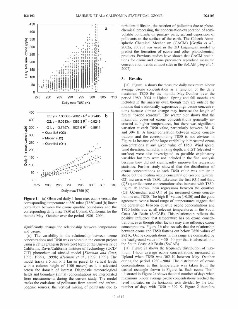
[12] Figure 1a shows the measured daily maximum 1-houraverage ozone concentration as a function of the dailymaximum T850 for the months May-October over theperiod 1980–2004 at Upland. Spring and fall months areincluded in the analysis even though they are outside themonths that traditionally experience high ozone concentra-tions because climate change may increase the length offuture ‘‘ozone seasons’’. The scatter plot shows that themaximum observed ozone concentrations generally in-creased at higher temperatures, but there was significantvariation at each T850 value, particularly between 281 Kand 304 K. A linear correlation between ozone concen-trations and the corresponding T850 is not obvious inFigure 1a because of the large variability in measured ozoneconcentrations at any given value of T850. Wind speed,wind direction, humidity, mixing depth, andDT (elevated –surface) were also investigated as possible explanatoryvariables but they were not included in the final analysisbecause they did not significantly improve the regressionstatistics. Further study showed that the distribution ofozone concentrations at each T850 value was similar inshape but the median ozone concentration (second quartile;Q2) increases with T850. Likewise, the first (Q1) and third(Q3) quartile ozone concentrations also increase with T850.Figure 1b shows linear regressions between the quartiles(Q3, Q2-median and Q1) of the measured ozone concen-trations and T850. The high R2 values (>0.80) and the goodagreement over a broad range of temperatures suggest thatthe correlation between quartile ozone concentrations andT850 holds true at all relevant temperatures in the SouthCoast Air Basin (SoCAB). This relationship reflects thepositive influence that temperature has on ozone concen-trations, even though other factors may also influence ozoneconcentrations. Figure 1b also reveals that the relationshipbetween ozone and T850 flattens out below T850 values of282 K. Ozone concentrations in this range are dominated bythe background value of �30–40 ppb that is advected intothe South Coast Air Basin (SoCAB).[13] Figure 2a shows the frequency distribution of max-

imum 1-hour average ozone concentrations measured atUpland when T850 was 302 K between May–Octoberduring the period 1980–2004. The distribution of ozoneconcentrations at this temperature was taken from thedashed rectangle shown in Figure 1a. Each ozone ‘‘bin’’illustrated in Figure 2a shows the total number of days whenmaximum 1-hour average ozone concentrations reached thelevel indicated on the horizontal axis divided by the totalnumber of days with T850 = 302 K. Figure 2 therefore

Figure 1. (a) Observed daily 1-hour max ozone versus thecorresponding temperature at 850 mbar (T850) and (b) linearcorrelation between the ozone quartile boundaries and thecorresponding daily max T850 at Upland, California, for themonths May–October over the period 1980–2004.


3 of 12

D21103

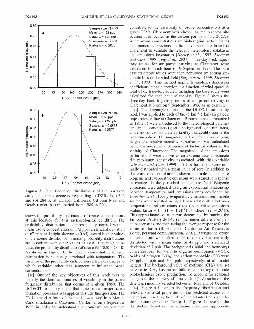
shows the probability distribution of ozone concentrationsat this location for this meteorological condition. Theprobability distribution is approximately normal with amean ozone concentration of 172 ppb, a standard deviationof 67 ppb, and slight skewness (0.65) toward higher valuesof the ozone distribution. Similar probability distributionsare associated with other values of T850. Figure 2b illus-trates the probability distribution of ozone for T850 = 284 K.As shown in Figure 1b, the median concentration of eachdistribution is positively correlated with temperature. Thevariance of the probability distribution reflects the degree towhich variables other than temperature influence ozoneconcentrations.[14] One of the key objectives of this work was to

identify the dominant sources of variability in the ozonefrequency distribution that occurs at a given T850. TheUCD/CIT air quality model that represents all major ozoneformation processes was applied to study this question. The2D Lagrangian form of the model was used in a Monte-Carlo simulation at Claremont, California, on 9 September1993 in order to understand the dominant sources that

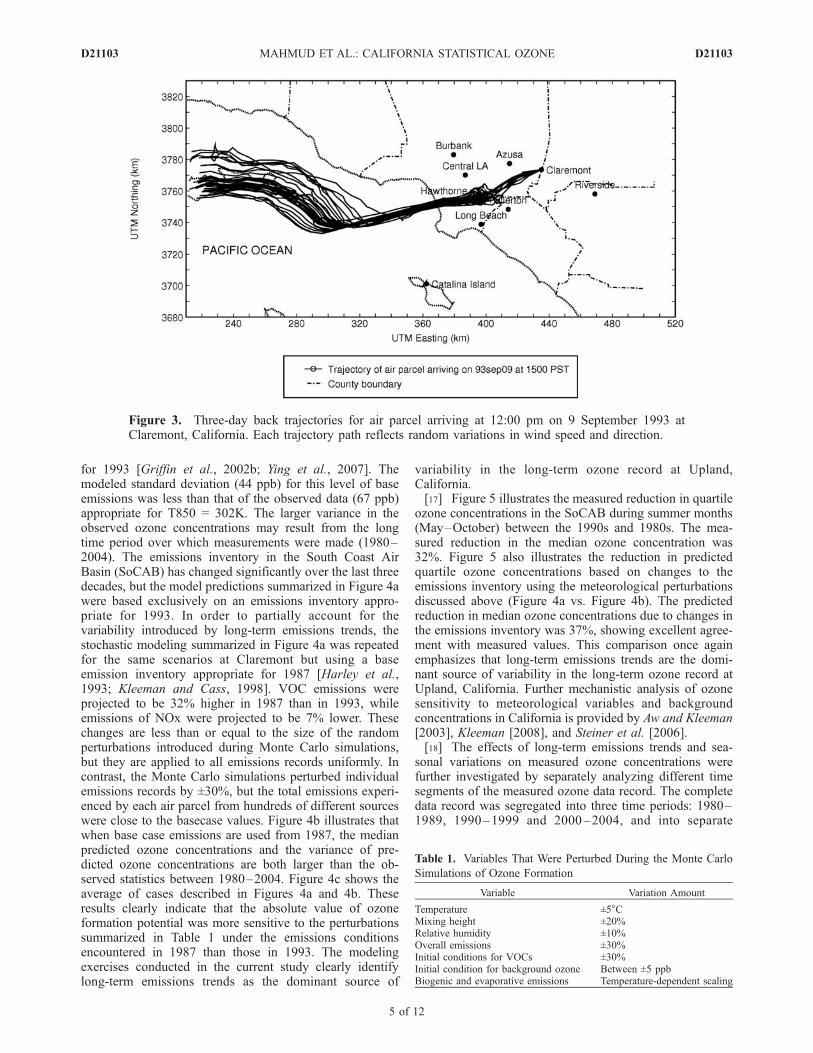
contribute to the variability of ozone concentrations at agiven T850. Claremont was chosen as the receptor sitebecause it is located in the eastern portion of the SoCABwhere ozone concentrations are highest (similar to Upland)and numerous previous studies have been conducted atClaremont to validate the relevant meteorology databasesand emissions inventories [Harley et al., 1993; Kleemanand Cass, 1998; Ying et al., 2007]. Three-day back trajec-tory routes for air parcel arriving at Claremont werecalculated for each hour on 9 September 1993. The basecase trajectory routes were then perturbed by adding sto-chastic bias to the wind-field [Bergin et al., 1999; Kleemanet al., 1999]. This method implicitly modifies dispersioncoefficients, since dispersion is a function of wind speed. Atotal of 62 trajectory routes, including the base route werecalculated for each hour of the day. Figure 3 shows thethree-day back trajectory routes of air parcel arriving atClaremont at 3 pm on 9 September 1993, as an example.[15] The Lagrangian form of the UCD/CIT air quality

model was applied to each of the (5 km * 5 km) air parcelstrajectories ending at Claremont. Perturbations (summarizedin Table 1) were introduced to the meteorological parame-ters, initial conditions (global background concentrations),and emissions to simulate variability that could occur in thereal atmosphere. The magnitude of the temperature, mixingheight and relative humidity perturbations was calculatedusing the measured distribution of historical values in thevicinity of Claremont. The magnitude of the emissionsperturbations were chosen as an extreme case to estimatethe maximum sensitivity associated with this variable[Kleeman and Cass, 1999b]. All perturbations were nor-mally distributed with a mean value of zero. In addition tothe emissions perturbations shown in Table 1, the basebiogenic and evaporative emissions were scaled in responseto changes in the perturbed temperature field. Biogenicemissions were adjusted using an exponential relationshipbetween temperature and emissions rates developed byGuenther et al. [1993]. Evaporative emissions from mobilesources were adjusted using a linear relationship betweentemperature and emissions rates (evaporative emissionsscaling factor = 1 + (T � Tref)*1.34 where Tref = 20�C).This approximate equation was determined by running theEmission FACtor (EMFAC) model under different temper-ature scenarios and then taking the average response for theentire air basin (B. Hancock, California Air ResourcesBoard, personal communication, 2007). Background ozoneconcentrations were taken to be random values normallydistributed with a mean value of 45 ppb and a standarddeviation of 5 ppb. The background (initial and boundary)concentrations for volatile organic compounds (VOC),oxides of nitrogen (NOX) and carbon monoxide (CO) were18 ppb, 2 ppb and 200 ppb, respectively, at all modelheights. The background value of methane (CH4) was setto zero as CH4 has no or little effect on regional-scalephotochemical ozone production. To account for seasonalchanges to the intensity of ultra violate (UV) radiation, thedate was randomly selected between 1 May and 31 October.[16] Figure 4 illustrates the frequency distribution and

relevant statistical properties of the predicted ozone con-centrations resulting from all of the Monte Carlo simula-tions summarized in Table 1. Figure 4a shows thedistribution based on the emission inventory appropriate

Figure 2. The frequency distributions of the observeddaily 1-hour max ozone corresponding to T850 of (a) 302and (b) 284 K at Upland, California, between May andOctober over the time period from 1980 to 2004.


4 of 12

D21103

for 1993 [Griffin et al., 2002b; Ying et al., 2007]. Themodeled standard deviation (44 ppb) for this level of baseemissions was less than that of the observed data (67 ppb)appropriate for T850 = 302K. The larger variance in theobserved ozone concentrations may result from the longtime period over which measurements were made (1980–2004). The emissions inventory in the South Coast AirBasin (SoCAB) has changed significantly over the last threedecades, but the model predictions summarized in Figure 4awere based exclusively on an emissions inventory appro-priate for 1993. In order to partially account for thevariability introduced by long-term emissions trends, thestochastic modeling summarized in Figure 4a was repeatedfor the same scenarios at Claremont but using a baseemission inventory appropriate for 1987 [Harley et al.,1993; Kleeman and Cass, 1998]. VOC emissions wereprojected to be 32% higher in 1987 than in 1993, whileemissions of NOx were projected to be 7% lower. Thesechanges are less than or equal to the size of the randomperturbations introduced during Monte Carlo simulations,but they are applied to all emissions records uniformly. Incontrast, the Monte Carlo simulations perturbed individualemissions records by ±30%, but the total emissions experi-enced by each air parcel from hundreds of different sourceswere close to the basecase values. Figure 4b illustrates thatwhen base case emissions are used from 1987, the medianpredicted ozone concentrations and the variance of pre-dicted ozone concentrations are both larger than the ob-served statistics between 1980–2004. Figure 4c shows theaverage of cases described in Figures 4a and 4b. Theseresults clearly indicate that the absolute value of ozoneformation potential was more sensitive to the perturbationssummarized in Table 1 under the emissions conditionsencountered in 1987 than those in 1993. The modelingexercises conducted in the current study clearly identifylong-term emissions trends as the dominant source of

variability in the long-term ozone record at Upland,California.[17] Figure 5 illustrates the measured reduction in quartile

ozone concentrations in the SoCAB during summer months(May–October) between the 1990s and 1980s. The mea-sured reduction in the median ozone concentration was32%. Figure 5 also illustrates the reduction in predictedquartile ozone concentrations based on changes to theemissions inventory using the meteorological perturbationsdiscussed above (Figure 4a vs. Figure 4b). The predictedreduction in median ozone concentrations due to changes inthe emissions inventory was 37%, showing excellent agree-ment with measured values. This comparison once againemphasizes that long-term emissions trends are the domi-nant source of variability in the long-term ozone record atUpland, California. Further mechanistic analysis of ozonesensitivity to meteorological variables and backgroundconcentrations in California is provided by Aw and Kleeman[2003], Kleeman [2008], and Steiner et al. [2006].[18] The effects of long-term emissions trends and sea-

sonal variations on measured ozone concentrations werefurther investigated by separately analyzing different timesegments of the measured ozone data record. The completedata record was segregated into three time periods: 1980–1989, 1990–1999 and 2000–2004, and into separate

Figure 3. Three-day back trajectories for air parcel arriving at 12:00 pm on 9 September 1993 atClaremont, California. Each trajectory path reflects random variations in wind speed and direction.

Table 1. Variables That Were Perturbed During the Monte Carlo

Simulations of Ozone Formation

Variable Variation Amount

Temperature ±5�CMixing height ±20%Relative humidity ±10%Overall emissions ±30%Initial conditions for VOCs ±30%Initial condition for background ozone Between ±5 ppbBiogenic and evaporative emissions Temperature-dependent scaling


5 of 12

D21103

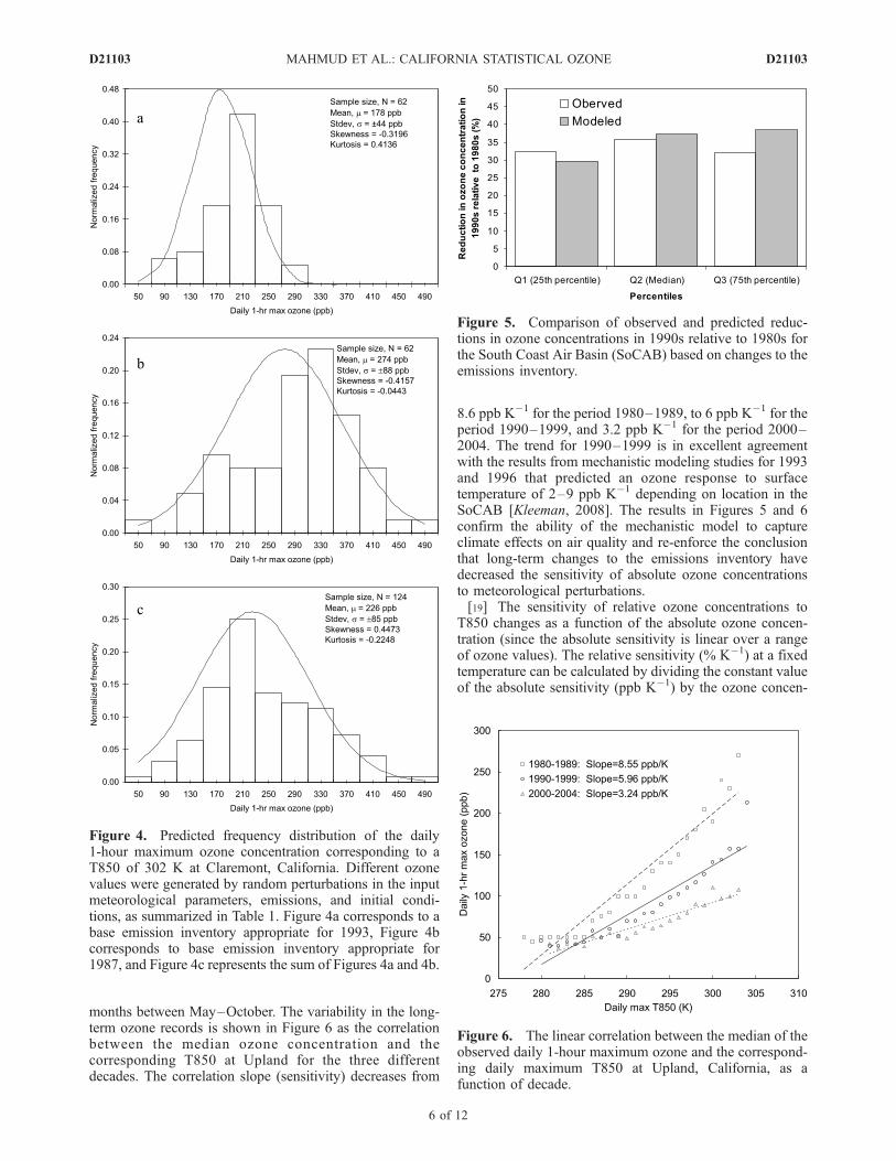
months between May–October. The variability in the long-term ozone records is shown in Figure 6 as the correlationbetween the median ozone concentration and thecorresponding T850 at Upland for the three differentdecades. The correlation slope (sensitivity) decreases from

8.6 ppb K�1 for the period 1980–1989, to 6 ppb K�1 for theperiod 1990–1999, and 3.2 ppb K�1 for the period 2000–2004. The trend for 1990–1999 is in excellent agreementwith the results from mechanistic modeling studies for 1993and 1996 that predicted an ozone response to surfacetemperature of 2–9 ppb K�1 depending on location in theSoCAB [Kleeman, 2008]. The results in Figures 5 and 6confirm the ability of the mechanistic model to captureclimate effects on air quality and re-enforce the conclusionthat long-term changes to the emissions inventory havedecreased the sensitivity of absolute ozone concentrationsto meteorological perturbations.[19] The sensitivity of relative ozone concentrations to

T850 changes as a function of the absolute ozone concen-tration (since the absolute sensitivity is linear over a rangeof ozone values). The relative sensitivity (% K�1) at a fixedtemperature can be calculated by dividing the constant valueof the absolute sensitivity (ppb K�1) by the ozone concen-

Figure 4. Predicted frequency distribution of the daily1-hour maximum ozone concentration corresponding to aT850 of 302 K at Claremont, California. Different ozonevalues were generated by random perturbations in the inputmeteorological parameters, emissions, and initial condi-tions, as summarized in Table 1. Figure 4a corresponds to abase emission inventory appropriate for 1993, Figure 4bcorresponds to base emission inventory appropriate for1987, and Figure 4c represents the sum of Figures 4a and 4b.

Figure 5. Comparison of observed and predicted reduc-tions in ozone concentrations in 1990s relative to 1980s forthe South Coast Air Basin (SoCAB) based on changes to theemissions inventory.

Figure 6. The linear correlation between the median of theobserved daily 1-hour maximum ozone and the correspond-ing daily maximum T850 at Upland, California, as afunction of decade.


6 of 12

D21103

tration (ppb) at the temperature of interest. Analysis of thedata shown in Figure 6 reveals that the sensitivity of relativeozone formation at T850 � 300 K is approximately constantat �4.3 % K�1 across each of the time periods that werestudied. When T850 < 300 K the calculated relative ozonesensitivity is influenced more strongly by the �30–40 ppbof background ozone that is transported into the air basin.Averaged across the entire range of temperatures illustratedin Figure 6, the relative sensitivity of ozone to temperaturedecreased from 6% K�1 in 1980–89 to 5.5% K�1 in 1990–99 and 4.3% K�1 in 2000–04. Overall, the sensitivity ofrelative ozone formation appears to be constant at hottertemperatures and decreasing at cooler temperatures acrossthe different time periods and emissions conditions studied.[20] Ozone precursor emissions have decreased from

1980–1989 levels because of improved technology andstringent emission control measures, producing a decreasingtrend in observed ozone concentrations [Cox et al., 2006].Future emissions changes may continue this downwardtrend, or they may rebound as population growth overtakesthe effects of increased efficiency. In either case, emissionswill be considered to be static at 1990–2004 levels for theremainder of the current study to allow for a direct analysisof climate change on ozone formation potential.[21] Figure 7 shows the linear regression between ozone

concentrations and Reanalysis T850 separately for different

summer months during the period 1990–2004 at Upland.The equations presented in the panels of Figure 7 representthe linear models based on the quartile ozone data. In eachpanel, the solid line represents the correlation based on themedian ozone concentration and the upper and lowerdashed lines indicate the correlation based on Q3 and Q1,respectively. The R2 values (>0.75) indicate that the aggre-gated statistics of the ozone concentration distribution andT850 are well correlated. Importantly, different slopes areobserved during different seasons. These reveal that ozoneresponds less strongly to temperature during the early spring(May– June) and late summer (September –October)months. Ozone concentrations respond most strongly totemperature during the middle of summer (July–August).The seasonal ozone response to T850 at Upland was alsoreanalyzed with a subset of the data points that have T850between 291 K–301 K. Values of T850 in this range weremeasured in all months June–September within the histor-ical data set, and so this analysis removes any potential biasassociated with temperature extremes experienced in onemonth but not other months. The ozone response within thecommon temperature range at Upland was still stronger inJuly–August vs. June or September, suggesting that someother seasonal factor besides temperature is influencing theresults. Monthly average mixing height measured between1984–1991 at Oakland, California (at the coast upwind of

Figure 7. Seasonal correlation between 1-hour maximum ozone and 1-hour maximum T850 at Upland,California, for the years between 1990 and 2004. Diamonds correspond to quartile 3 (Q3), squarescorrespond to quartile 2 (median; Q2), and triangles correspond to quartile 1 (Q1).


7 of 12

D21103

the SJVAB) varied from 660 ± 80 m (June), 550 ± 75 m(July), 620 ± 74 m (August), and 660 ± 150 m (September).Mixing depth can influence ozone production [Kleeman,2008], but the inclusion of the best-available mixing depthinformation in the current study did not add skill to thestatistical model. Another possible seasonal factor is trendsin biogenic emissions as vegetation follows a seasonalgrowth cycle [see for example Geron et al., 2000].[22] Figure 8 shows the linear regression of quartile

ozone concentrations from Reanalysis T850 at Parlier inthe SJVAB for each month between May–October. Ozonetrends in the SJVAB are qualitatively similar to those in theSoCAB, but the magnitude of the change induced bytemperature is different because the underlying emissionsinventories for the two air basins are not the same. Increasedtemperature still enhances ozone concentrations in theSJVAB, but the magnitude of the change is smaller thanthat observed in the SoCAB. As exhibited by the Uplandanalyses, July and August had the largest values of theregression slopes between ozone and T850 compared toother months.[23] Future trends in upper air temperature are simulated

by Global Climate Models (GCMs) in response to globalchange. There are several climate models currently availablein the scientific community including the National Centerfor Atmospheric Research Parallel Climate Model version 1

(NCAR-PCM1), the NCAR-Community Climate SystemModel version 3 (NCAR-CCSM3), the Geophysical FluidDynamics Coupled Model version 2.1 (GFDL CM2.1), theCentre National de Recherches Meteorologiques ClimateModel version 3 (CNRM-CM3) (French climate model), theMax Planck Institute for Meteorology ECHAM version 5(MPI-ECHAM5) (German climate model), and the Modelfor Interdisciplinary Research on Climate version 3.2(MIROC3.2) (medium resolution) (Japanese climate model).In the current study, the GFDL CM2.1 model was used toprovide simulated T850 over a global domain, includingCalifornia, for the years 2001–2100 based on several IPCCgreenhouse gas emissions scenarios. Table 2 summarizes thetemperature (T850) increase in California over the period2070–2099 relative to 1961–1990 predicted by all of theGCMs described above. Decadal average results for allmodels are similar with a temperature increase of 4–5�C(A2 highest-emission scenario) or 3–4�C (B1 lowest-emis-sions scenario) during the summer ozone season in both theSJVAB and the SoCAB. The daily GFDL CM2.1 values ofT850 simulated at coarse scale from model locations overthe SoCAB and the SJVAB under the A2 and the B1scenarios were used to estimate the potential for ozoneformation in California. Ozone concentrations at Uplandand Parlier were calculated based on the projected values ofT850 for each day and the monthly statistical relationships

Figure 8. Seasonal correlation between 1-hour maximum ozone and 1-hour maximum T850 at Parlier,California, for the years between 1990 and 2004. Diamonds correspond to quartile 3 (Q3), squarescorrespond to quartile 2 (median; Q2), and triangles correspond to quartile 1 (Q1).


8 of 12

D21103

between ozone and T850 illustrated in Figures 7 and 8 forthe period 1990–2004. The median (Q2) ozone-T850relationship in Figures 7 and 8 were used to obtain abaseline estimate, while Q1 and Q3 were used to obtainupper and lower bounds. In addition to the summer months(May–Oct), the correlations found in May and Octoberwere applied to each month of the periods February–April,and November–January, respectively. After calculating thedaily 1-hour max quartile (Q1, Q2 and Q3) ozone concen-trations with the projected temperature values for each year,the number of days with 90 ppb or more ozone wascalculated for each month and an aggregate yearly result

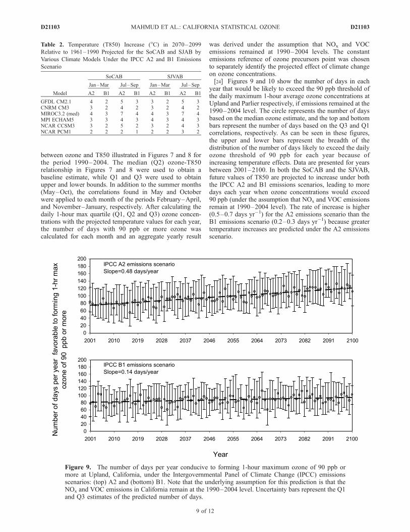
was derived under the assumption that NOx and VOCemissions remained at 1990–2004 levels. The constantemissions reference of ozone precursors point was chosento separately identify the projected effect of climate changeon ozone concentrations.[24] Figures 9 and 10 show the number of days in each

year that would be likely to exceed the 90 ppb threshold ofthe daily maximum 1-hour average ozone concentrations atUpland and Parlier respectively, if emissions remained at the1990–2004 level. The circle represents the number of daysbased on the median ozone estimate, and the top and bottombars represent the number of days based on the Q3 and Q1correlations, respectively. As can be seen in these figures,the upper and lower bars represent the breadth of thedistribution of the number of days likely to exceed the dailyozone threshold of 90 ppb for each year because ofincreasing temperature effects. Data are presented for yearsbetween 2001–2100. In both the SoCAB and the SJVAB,future values of T850 are projected to increase under boththe IPCC A2 and B1 emissions scenarios, leading to moredays each year when ozone concentrations would exceed90 ppb (under the assumption that NOx and VOC emissionsremain at 1990–2004 level). The rate of increase is higher(0.5–0.7 days yr�1) for the A2 emissions scenario than theB1 emissions scenario (0.2–0.3 days yr�1) because greatertemperature increases are predicted under the A2 emissionsscenario.

Figure 9. The number of days per year conducive to forming 1-hour maximum ozone of 90 ppb ormore at Upland, California, under the Intergovernmental Panel of Climate Change (IPCC) emissionsscenarios: (top) A2 and (bottom) B1. Note that the underlying assumption for this prediction is that theNOx and VOC emissions in California remain at the 1990–2004 level. Uncertainty bars represent the Q1and Q3 estimates of the predicted number of days.

Table 2. Temperature (T850) Increase (�C) in 2070–2099

Relative to 1961–1990 Projected for the SoCAB and SJAB by

Various Climate Models Under the IPCC A2 and B1 Emissions

Scenario

SoCAB SJVAB

Jan–Mar Jul–Sep Jan–Mar Jul–Sep

Model A2 B1 A2 B1 A2 B1 A2 B1

GFDL CM2.1 4 2 5 3 3 2 5 3CNRM CM3 3 2 4 2 3 2 4 2MIROC3.2 (med) 4 3 7 4 4 3 7 4MPI ECHAM5 3 3 4 3 4 3 4 3NCAR CCSM3 3 2 5 2 3 2 4 3NCAR PCM1 2 2 2 1 2 2 3 2


9 of 12

D21103

[25] The rate of increase for the number of days exceed-ing the 90 ppb ozone threshold at Parlier (SJVAB) is greaterthan at Upland (SoCAB) despite the fact that historicalozone concentrations are less sensitive to temperature at

Parlier during all months but October (compare Figure 7 toFigure 8). These apparently contradictory trends can beexplained by examining the total number of days exceeding90 ppb of ozone during each month of the years 2046–2055

Figure 10. The number of days per year conducive to forming 1-hour maximum ozone of 90 ppb ormore at Parlier, California, under the Intergovernmental Panel of Climate Change (IPCC) emissionsscenarios: (top) A2 and (bottom) B1. Note that the underlying assumption for this prediction is that theNOx and VOC emissions in California remain at the 1990–2004 level. Uncertainty bars represent the Q1and Q3 estimates of the predicted number of days.

Figure 11. Number of days per decade conducive to the formation of daily 1-hour max ozone�90 ppb for2046–2055 and 2091–2100 at Upland (SoCAB) and Parlier (SJVAB). Note that the underlying assumptionfor this prediction is that the NOx and VOC emissions in California remain at the 1990–2004 level.


10 of 12

D21103

and 2091–2100 assuming emissions remained at 1990–2004 levels. Figure 11 illustrates that the months of July andAugust become ‘‘saturated’’ after �2050 with continuedincreases occurring mainly in May–June and September–October. The annual growth at Parlier (SJVAB) is greaterthan Upland (SoCAB) primarily because of increases duringthe month of October. These trends reflect the greaterlengthening of the ‘‘ozone season’’ in the SJVAB comparedto the SoCAB assuming emissions remained constant at1990–2004 levels.[26] Table 3 illustrates the predicted seasonal (May–

October) median daily 1-hour ozone concentration for eachdecade over the period 2001–2100 at Upland (SoCAB) andParlier (SJVAB) under the IPCC A2 and B1 emissionsscenarios. Generally, the predicted median ozone increasesin both the SoCAB and SJVAB over time. The seasonalmedian daily 1-hour ozone concentration would exceed90 ppb as early as in 2031–2040 under the warminginduced by the A2 global emissions scenario assumingNOx and VOC emissions in California remain at the1990–2004 level. Global Climate Models are not expectedto accurately represent the weather during any given yearbut they should capture the meteorology over a period ofdecades. The GFDL CM2.1 model results were obtained forthe period 1990–2000 and the T850 values were used topredict ozone concentrations based on the correlationsderived in the current study. The average value of the 1-hourmaximum daily ozone concentration was 84 ppb (predicted)vs. 97 ppb (measured) in the SoCAB and 83 ppb (predicted)vs. 85 ppb (measured) in the SJVAB for this period indicatingthat the statistical downscaling method developed in thisstudy can effectively be used to project ozone concentrationsin the future for a given air basin.

4. Conclusion

[27] The daily maximum upper air temperature at analtitude of 850-mbar pressure (T850) taken from coarse-scale global model locations nearest to California’s twomost polluted air basins can be used to model daily 1-hourmaximum surface ozone concentrations in those air basins.Other explanatory variables including wind speed, winddirection, humidity, and mixing depth did no add skill to the

statistical model. There is not a one-to-one correlationbetween ozone and T850 extracted from the global Reanal-ysis data set, but the value of T850 can be used to predictthe statistical properties of the possible range of ozoneconcentrations. These ozone concentration distributionsare approximately normal and their 25%, 50% and 75%quartile concentrations are linearly correlated with temper-ature. By constructing separate linear regression models foreach month of the year, the effects of seasonal changes onthe ozone – T850 relationship can be represented. Theresponse of ozone to T850 is strongest in July and Augustand weaker in spring, early summer and fall. The sensitivityof absolute ozone concentrations to T850 has decreasedover the past several decades because of changes in anthro-pogenic emissions. Future anthropogenic emissions trendsin California will depend on the balance between populationgrowth vs. energy conservation and the further developmentof efficient technologies.[28] The statistical relationship between coarse-scale

T850 and fine-scale ozone concentrations provides anefficient technique to downscale global model circulationstructure to local air basin ozone concentrations. The effectof climate on future ozone concentrations can be evaluatedusing average emissions levels between 1990–2004 as aconstant reference point. Projections of future temperaturemade by the GFDL CM2.1 global climate model combinedwith the historical ozone trends suggest that, by the year2050, the number of days with conditions likely to encour-age ozone concentrations greater than 90 ppb would in-crease by 22–30 days yr�1 under the IPCC SRES A2emissions scenario and 6–13 days yr�1 under the B1emissions scenario. Warmer future temperatures will requirethe implementation of additional emissions controls inCalifornia to offset this climate ‘‘penalty’’.

[29] Acknowledgments. This research was supported by the Califor-nia Air Resources Board Project 04-349. D.R.C. and M.T. were funded bythe California Energy Commission through the California Climate ChangeCenter and by the NOAA RISA program through the California Applica-tions Program. We thank Martha Coakley and Josh Shiffrin for dataprocessing and analyses.

ReferencesAw, J., and M. J. Kleeman (2003), Evaluating the first-order effect ofintraannual temperature variability on urban air pollution, J. Geophys.Res., 108(D12), 4365, doi:10.1029/2002JD002688.

Bell, M. L., et al. (2007), Climate change, ambient ozone, and health in 50US cities, Clim. Change, 82, 61–76.

Bergin, M. S., et al. (1999), Formal uncertainty analysis of a Lagrangianphotochemical air pollution model, Environ. Sci. Technol., 33, 1116–1126.

Cayan, D. R., et al. (2008), Climate change scenarios for the Californiaregion, Clim. Change (Special Issue on Climate Change Scenarios), 87,S21–S42.

Constable, J. V. H., et al. (1999), Modelling changes in VOC emission inresponse to climate change in the continental United States, GlobalChange Biol., 5, 791–806.

Cox, P., et al. (2006), The California Almanac of Emissions and Air Qual-ity, Plann. and Tech. Support Div. Calif. Air Resour. Board, Sacramento,CA.

Dawson, J. P., et al. (2007), Sensitivity of ozone to summertime climate inthe eastern USA: A modeling case study, Atmos. Environ., 41, 1494–1511.

Delworth, T. L., et al. (2006), GFDL’s CM2 global coupled climatemodels. part I: Formulation and simulation characteristics, J. Clim.,19, 643–674.

Fuentes, J. D., et al. (2000), Biogenic hydrocarbons in the atmosphericboundary layer: A review, Bull. Am. Meteorol. Soc., 81, 1537–1575.

Table 3. Summary of Predicted Decadal Median Daily 1-Hr

Maximum Ozone Concentrations Under IPCC A2 and B1 Global

Emissions Scenarios at Upland (SoCAB) and Parlier (SJVAB)a

Median Ozone Concentration (ppb)

Upland (SoCAB) Parlier (SJVAB)

Decade A2 B1 A2 B1

2001–2010 84 84 86 872011–2020 84 87 87 872021–2030 86 86 88 862031–2040 92 87 90 892041–2050 90 87 90 892051–2060 92 87 92 882061–2070 97 89 93 912071–2080 100 91 96 902081–2090 105 92 97 912091–2100 111 91 101 92

aNote that the underlying assumption for this prediction is that the NOx

and VOC emissions in California remain at the 1990–2004 level.


11 of 12

D21103

Geron, C., et al. (2000), Temporal variability in basal isoprene emissionfactor, Tree Physiol., 20, 799–805.

Griffin, R. J., et al. (2002a), Secondary organic aerosol—3. Urban/regionalscale model of size- and composition-resolved aerosols, J. Geophys. Res.,107(D17), 4334, doi:10.1029/2006JD000544.

Griffin, R. J., et al. (2002b), Secondary organic aerosol—1. Atmosphericchemical mechanism for production of molecular constituents, J. Geo-phys. Res., 107(D17), 4332, doi:10.1029/2001JD000541.

Guenther, A. B., et al. (1993), Isoprene and monoterpene emission ratevariability—Model evaluations and sensitivity analyses, J. Geophys.Res., 98, 12,609–12,617.

Harley, R. A., et al. (1993), Photochemical modeling of the Southern Ca-lifornia air-quality study, Environ. Sci. Technol., 27, 378–388.

Hogrefe, C., et al. (2004), Simulating changes in regional air pollution overthe eastern United States due to changes in global and regional climateand emissions, J. Geophys. Res., 109, D22301, doi:10.1029/2004JD004690.

Kalnay, E., et al. (1996), The NCEP/NCAR 40-year reanalysis project, Bull.Am. Meteorol. Soc., 77, 437–471.

Kleeman, M. J. (2008), A preliminary assessment of the sensitivity of airquality in California to global change, Clim. Change, 87, suppl. 1, 273–292.

Kleeman, M. J., and G. R. Cass (1998), Source contributions to the size andcomposition distribution of urban particulate air pollution, Atmos. Environ.,32, 2803–2816.

Kleeman, M. J., and G. R. Cass (1999a), Effect of emission control strate-gies on the size and composition distribution of urban particulate airpollution, Environ. Sci. Technol., 33, 177–189.

Kleeman, M. J., and G. R. Cass (1999b), Identifying the effect of individualemissions sources on particulate air quality within a photochemical aero-sol processes trajectory model, Atmos. Environ., 33, 4597–4613.

Kleeman, M. J., G. R. Cass, and A. Eldering (1997), Modeling the airborneparticle complex as a source-oriented external mixture, J. Geophys. Res.,102(D17), 21,355–21,372.

Kleeman, M. J., et al. (1999), Source contributions to the size and composi-tion distribution of atmospheric particles: Southern California in Septem-ber 1996, Environ. Sci. Technol., 33, 4331–4341.

Rubin, J. I., et al. (2006), Temperature dependence of volatile organiccompound evaporative emissions from motor vehicles, J. Geophys.Res., 111, D03305, doi:10.1029/2005JD006458.

Sanderson, M. G., et al. (2003), Effect of climate change on isopreneemissions and surface ozone levels, Geophys. Res. Lett., 30(18), 1936,doi:10.1029/2003GL017642.

Seinfeld, J. H., and S. N. Pandis (2006), Atmospheric Chemistry and Phy-sics: From Air Pollution to Climate Change, Wiley, New York.

Sillman, S., and F. J. Samson (1995), Impact of temperature on oxidantphotochemistry in urban, polluted rural and remote environments,J. Geophys. Res., 100(D6), 11,497–11,508.

Snyder, M. A., et al. (2004), Modeled regional climate change in the hy-drologic regions of California: A CO2 sensitivity study, J. Am. WaterResour. Assoc., 40, 591–601.

Steiner, A. L., et al. (2006), Influence of future climate and emissions onregional air quality in California, J. Geophys. Res., 111, D18303,doi:10.1029/2005JD006935.

Ying, Q., et al. (2007), Verification of a source-oriented externally mixed airquality model during a severe photochemical smog episode, Atmos. En-viron., 41, 1521–1538.

��D. Cayan and M. Tyree, Scripps Institute of Oceanography, University of

California, San Diego, La Jolla, San Diego, CA 92093, USA.M. J. Kleeman and A. Mahmud, Department of Civil and Environmental

Engineering, University of California, Davis, 1 Shields Avenue, Davis, CA95616, USA. ([email protected])N. Motallebi, Research Division, California Air Resources Board,

Sacramento, CA 95812, USA.


12 of 12

D21103

statistical downscaling of climate change impacts on...

Documents