standard local labor demand manacorda - ucw project · local labor demand and child labor m....
TRANSCRIPT
1.
Local labor demand and child labor
M. ManacordaF. C. Rosati
March 2007
Und
erst
andi
ng C
hild
ren’
s Wor
k Pr
ojec
t Wor
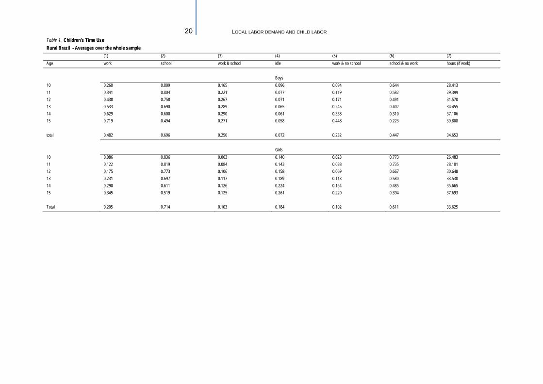
king
Pap
er S
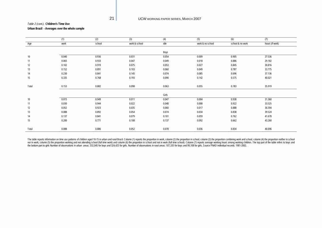
erie
s, M
arch
200
7

Local labor demand and child labor
M. Manacorda*
F. C. Rosati**
Working Paper March 2007
Understanding Children’s Work (UCW) Project
University of Rome “Tor Vergata” Faculty of Economics
V. Columbia 2, 00133 Rome
Tel: +39 06.7259.5618 Fax: +39 06.2020.687
Email: [email protected]
As part of broader efforts toward durable solutions to child labor, the International Labour Organization (ILO), the United Nations Children’s Fund (UNICEF), and the World Bank initiated the interagency Understanding Children’s Work (UCW) project in December 2000. The project is guided by the Oslo Agenda for Action, which laid out the priorities for the international community in the fight against child labor. Through a variety of data collection, research, and assessment activities, the UCW project is broadly directed toward improving understanding of child labor, its causes and effects, how it can be measured, and effective policies for addressing it. For further information, see the project website at www.ucw-project.org.
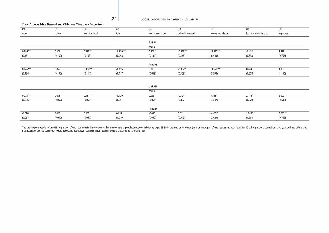
This paper is part of the research carried out within UCW (Understanding Children's Work), a joint ILO, World Bank and UNICEF project. The views expressed here are those of the authors' and should not be attributed to the ILO, the World Bank, UNICEF or any of these agencies’ member countries.
* Department of Economics, QMUL, Centre for Economic Performance and STICERD, LSE and CEPR ** UCW project and Univerisity of Rome “Tor Vergata”
Local labor demand and child labor
Working Paper No. 187 March, 2002
ABSTRACT
This paper uses micro data from the Brazilian PNAD between 1981 and 2002 to ascertain the role that local labor demand – proxied by male adult employment in the area of residence - plays in shaping the work and schooling decisions of children aged 10-15. Contrary to the widespread view that child labor is procyclical, we find evidence that employment (schooling) falls (increases) among young children (aged 10-12) when local labor demand is stronger. This result is consistent with the view that children's work is to a large extent the result of poverty, and that parents want to protect their children from child labor and do so if offered the opportunity.
Local labor demand and child labor
Working Paper March 2007
CONTENTS
Introduction ....................................................................................................................... 1 1. Local labor demand and child labor ...................................................................... 2 2. Data and descriptive information .......................................................................... 3 3. Empirical analysis.................................................................................................. 7
3.1 Basic evidence ....................................................................................................... 7 3.2 Basic regressions ................................................................................................... 7 3.3 Controls for observable characteristics .................................................................. 9 3.4 Controlling for migration ..................................................................................... 10 3.5 Differential responses by household income ....................................................... 11 3.6 Differential responses across age groups ............................................................. 12
4. Conclusions ......................................................................................................... 14 Appendix ......................................................................................................................... 15
A. A simple model of labor supply and schooling ................................................... 15

1 UCW WORKING PAPER SERIES, MARCH 2007
1. INTRODUCTION 1. Theory predicts that demand for and the returns to child work are important determinants of household decisions about children’s time use. Their role, however, has been subject to only limited empirical assessment (see Edmonds, 2007, for a review of the existing literature on local labor markets and child labor). Demand and returns from child work are typically difficult to measure especially as wages are observable only for a minority of children2 and labor market imperfections prevent sound imputations. The way that households respond in terms of their children's time use to labor market incentives has, on the other hand, relevant policy implications. Policy focus has been mainly targeted to improving access to school or to relaxing household resource constraints. However, such interventions might not be the most relevant in situations where labor demand is driving household decisions. Moreover, policy effectiveness might be reduced by behavioral responses; for example, policies aimed at lifting households out of poverty via labor demand boosting interventions might eventually end up harming children by increasing their incentives for work and early school drop out. 2. In this paper we exploit changes in the male adult employment in the area of residence to identify children's (aged 10-15) labor supply and schooling responses to variations in local labor demand. We use micro data from the Brazilian Pesquisa Nacional Por Amostra de Domicílios (PNAD) 1981-2002. 3. Economic theory leads to ambiguous predictions on the effect of a rise in local labor demand on children's time use.3 In fact, a stronger labor market is likely to generate both income and substitution effects, which might push in opposite directions. To the extent that improved labor market conditions generate higher earnings for adults and leisure (schooling) is a normal good, children's labor market participation should fall.4 On the other hand, if they are also associated with an increase in children's wages (and we will show that this is the case), this might lead to a rise in children's labor market participation. These effects are likely to be differentiated depending on the characteristics of the household and of the child. For example, the level of household income is likely to influence the relative size of income and substitution effects. Similarly, child productivity, returns to investment in their human capital and parental preferences over their children's time use are likely to be differentiated by age and gender. 4. We are not first ones to investigate empirically the effect of changes in local labor demand on children's time allocation (see the next section), but we will extend previous work by allowing for heterogeneous responses to changes in local labor market conditions. A consensus seems to have emerged in the empirical literature around the idea that children's labor supply increases in better times. Although not at all inconsistent with the standard textbook model of labor supply, this immediately raises serious concerns about a potential misalignment between children's and parents' interests (see Udry, 2004 on this). Similarly, this finding seems to contradict the idea that child labor is the result of extreme poverty. If parents would rather shelter their children from work but they are forced to engage them in productive activities out of
2 Most children do not work for a wage, but in their household farm or business. In these circumstances, labor market imperfection requires complex approaches in order to estimates the (shadow) contribution of children’s to household income (see Menon et al. 2005). 3 For a reference theoretical model see Cigno and Rosati, 2005. 4 Although school attendance might not necessarily fall due to substitution between adult and children’s time in household chores.
2 LOCAL LABOR DEMAND AND CHILD LABOR
destitution (as in Basu and Van, 1998), one would expect child labor to fall when both parents' and children's labor market opportunities improve. 5. Similar to the findings of others, our empirical analysis shows that in better times children aged 10-15 tend on average to work more, being more likely to combine work with school and less likely to be inactive. This result however masks substantial heterogeneity across groups. The very large sample size of our dataset (around one million observations) allows us to investigate with some precision differences in responses across different types of children. It is rural children and those who belong to poorer households who largely increase their labor supply in response to better labor market conditions. Among richer children the reverse happens, with improvements in local labor markets leading to a rise in school attendance and a fall in labor market participation. Our more novel result, however, is that younger children tend to cut their labor supply and increase school enrollment when labor demand is stronger. It is only at around ages 12 or 13 that young Brazilians start to behave like adults in the labor market. Hence, contrary to the widespread view that in better times children work more and drop out of school, we show that for young children the reverse happens. This is consistent with a simple model where child labor and schooling are the result of extreme poverty. Effects of labor market stance on relative returns to work differentiated by gender, area of residence and, especially, age and parental preferences for children's leisure and schooling (rather than labor market incentives) changing rapidly as the child grows are likely to explain these results. Our results strongly suggest - perhaps unsurprisingly - that some care must be exerted in pooling children of different ages together when dealing with child labor issues. 6. The organization of the paper is as follows. Section I briefly discusses the likely implications of a temporary increase in labor demand on children's work and school decisions and reviews the literature in this area. Section II introduces the data and presents basic evidence on child labor and schooling in Brazil. Section III presents the empirical estimates. Section IV discusses the results and concludes.
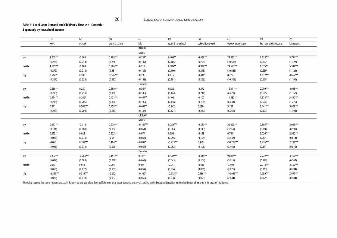
2. LOCAL LABOR DEMAND AND CHILD LABOR 7. Theory yields ambiguous predictions on an improvement in the state of the local labor market on young individuals' labor supply and school enrollment decisions. 8. To fix ideas, consider a simple labor supply model where households maximize a utility function that depends on consumption, children's leisure and schooling. Children can work for a market wage (we ignore work on the household farm) and school is costly. The technical appendix reports the equilibrium given a specific functional form for the utility function. 9. Consider a temporary exogenous increase in labor demand. One would expect adult wages to increase. Unless the elasticity of adults' labor supply is negative, one would expect both parents' employment and earnings to increase. If children's leisure (schooling) is a normal good, one would expect children's labor market participation to fall a result. The effect is reinforced if households have more than one child. In this case a rise in one child's labor income might go to the advantage of this child's siblings, further contributing to a reduction in child labor (Manacorda, 2006). 10. If an increase in labor demand also leads to a rise in children's market wages, this is deemed to have the opposite effect on children's time use due to a classical substitution effect. By increasing the opportunity cost of both school and leisure, one would expect a rise in children's labor market participation. The effect might be tempered or even reverted if parents attach a high utility to schooling and schooling is
3 UCW WORKING PAPER SERIES, MARCH 2007
costly or if the disutility of work is sufficiently high. In a world where there are direct costs of attending school, part of the increased earnings accruing to working children from higher market wages might go into purchasing more schooling. In this case schooling in combination with work might increase, leading potentially to an overall rise in school attendance. Similarly, if the disutility of children's work is sufficiently high, a rise in children's market wages will lead to a fall in children's labor supply (at the intensive margin) and no rise in participation. This would happen for example if schooling/leisure is a luxury and children only work up to the point where the household reaches a subsistence consumption level as in Basu and Van's (1998). 11. There is no lack of empirical evidence on the effect of increases in local labor demand on young children's labor supply and school enrollment in developing countries. Parikh and Sadoulet (2005) for example find a positive association between local area employment and work using a cross sectional of Brazilian (PNAD) data. Similar results are found by Guarcello et al. (2006) for Ethiopia and Manacorda and Kondylis (2006) for Tanzania. In a recent paper on Brazil that uses the same data as the ones used in this study, Krueger (2007) uses the variation in the value of coffee production across Brazilian counties and time to measure changes in local economic conditions. She shows that an increase in the value of coffee production induces a fall in school attendance and a rise in child labor among children of parents with low and intermediate levels of education. 12. The evidence that youth and adult employment covary positively and that young individuals tend to work more in periods of stronger labor demand is largely in line with work on youths and teenagers in the labor markets, most of which is based on data from developed countries. These studies show that young individuals' employment (schooling) responds positively (negatively) to improvement in local labor market conditions and that youths are particularly responsive to the state of the economic cycle (Blanchflower, 1999, Blanchflower and Freeman, 2000a, 2000b; Card and Lemieux, 2000; Eckstein and Wolpin, 1999; Freeman and Rodgers, 1999; Freeman and Wise, 1982; ILO, 2000; OCED, 1996, 1998, 1999; Rees, 1986). 13. Other papers examine separately improvements in children's market wages and household income. Based on the same data used in this paper, Duryea and Arends-Kuenning (2003) find that a rise in unskilled wages leads to an increase in urban teenagers’ (ages 14-16) employment, consistent with a simple model of labor supply but inconsistent with the idea that the leisure/schooling of these children is a luxury good (in which case labor supply should fall). Several pieces of research also convincingly show that improvements in household resources and living standards lead to a fall in child labor (see for example Edmonds, 2005 and 2006), and that negative shocks to household income lead to increased work participation and lower school attendance among children (Duryea and Arends-Kuenning, 2003), in turn suggesting that child leisure/schooling is a normal (not necessarily a luxury) good.
3. DATA AND DESCRIPTIVE INFORMATION 14. In the rest of this paper we examine more closely children's labor supply responses to changes in local labor demand in Brazil. We use micro data from the PNAD for the period 1981 to 2002. PNAD is a household survey run annually (with the exception of 1991, 1994 and 2000) that is representative of the entire Brazil except the rural North-West. The survey collects detailed individual and household socio economic characteristics as well as information on work activity and school enrolment consistently throughout the sample period. Labor market data are available throughout the whole period only for individuals aged 10 or older and include
4 LOCAL LABOR DEMAND AND CHILD LABOR
information on hours of work in the week preceding the survey. Work refers to both paid and unpaid (family or non family) work but excludes household chores. Data on labor earnings are only available for paid workers, a minority of working children especially in rural areas. 15. We focus our analysis on individuals aged 10-15. We have an overall sample of around one million children-observations over 19 waves: about three fourths in urban areas and one fourth in rural areas. This large sample size allows us to investigate in some detail heterogeneous responses across gender, residence and other characteristics of children, and potentially to shed some light on the role that constraints, opportunities and preferences play in shaping children's time use decisions in Brazil. 16. Table 1 presents descriptive data on children's time use. Column 1 presents the proportion of those currently involved in economic activities (work), column 2 the proportion enrolled in school, column 3 the proportion of individuals combining work and school, column 4 the proportion devoting no time to either of these activities, column 5 the proportion of children in work and not in school (working only) and column 6 the proportion of those in school and not in work (attending school only). Finally, column 7 reports working hours for those who work. The data are averages over the entire period of observation for the whole of Brazil. 17. As already shown by others (see for example World Bank, 2001b), children's work involvement is far from trivial in Brazil. Over the sample period, on average 48% of rural boys age 10-15 were in work and 70% were in school. Since these two figures add up to more than 100%, it is evident that a certain proportion of children combine work with school. This is illustrated in column 3, where one can see that around 25% of rural boys devote time to both activities. Despite a high probability of combining work with school, a significant proportion of children are classified as inactive, i.e. neither working nor attending school. For rural boys this proportion is in the order of 7%. Because 48% of children are in work and around 25% combine work and school, it follows that the residual 23% works only (column 5). Similarly, given that 70% are in school, the proportion attending school only is around 45% as shown in column 6. Hours of work among working children are remarkably high and in the order of 35 hours per week, almost a full time schedule over 5 days a week. Trends over age show, as expected, that as children grow older they tend increasingly to work, leaving school and inactivity. If anything, the proportion combining work and school rises modestly with age, implying that the increase in work participation happens at a faster rate than the fall in school attendance. 18. Results for rural girls are qualitatively similar. Girls though are much less likely than boys to be in work (21% versus 48%), less likely to combine work and school (10% versus 25%) and more likely to be in school only (60% versus 43%). With respect to boys, girls are also more likely to be inactive (18% versus 5%), although this masks a higher involvement in household chores. Trends over age are similar between the two gender groups, with the exception of inactivity. As girls leave school, an increasing proportion goes into inactivity (or household chores), in contrast to boys who get gradually absorbed into the labor market. 19. An analysis of urban children shows that urban boys are less likely to work (15% versus 48%) and are more likely to attend school (88% versus 70%) than rural children. Combining work and school also appears an option less often pursued by urban children compared to rural ones (10% versus 25%). Lower work involvement of urban children is presumably due to both higher living standards in urban areas compared to rural ones together with the circumstance that urban boys are not able to combine a flexible work schedule on the household farm with school attendance, one
5 UCW WORKING PAPER SERIES, MARCH 2007
option likely to be pursued by rural children. There are no appreciable differences between urban and rural boys in the proportion inactive or in the number of working hours. Trends over age are also similar with the notable exception of inactivity that falls with age for rural boys while it increases with age for urban boys. This suggests that non-enrollment among young children in rural areas is unlikely to be completely explained by their need to work. As they grow older, rural children do not appear to be short of employment opportunities, most likely on the household farm (hence potentially in rather unproductive jobs). In contrast, urban boys who leave school appear to be somewhat constrained in their employment opportunities. This should be no surprise if urban jobs provide better pay than rural ones: a simple Harris-Todaro (1970) model predicts that urban unemployment will arise (when urban wages are rigid) to keep the labor market in equilibrium. 20. Differences between girls and boys in urban labor markets are similar to the ones found in rural areas. Again, relative to boys, urban girls tend to work less (9% versus 15%), are less likely to combine work with school (5% versus 10%) and are slightly more likely to be inactive (8% versus 6%). Trends over age are remarkably similar across gender groups. 21. Although Table 1 gives a good indication of the average labor market outcomes of Brazilian children between 1981 and 2002, it also masks substantial heterogeneity in children's time use both over time and across areas. 22. Figures 1 to 3 plot time trends in children's time use between 1981 and 2002. As data across decades are not strictly comparable, given changes in the way the work variable is recorded and an overall change in the sampling scheme5 , some care must be exerted in making comparisons across decades. The main trends are not, however, affected by such discontinuities. 23. Figure 1 plots the proportion of children in work in each year, distinguishing between those in full time work and those combining work with school. During the 1980s child labor remains unchanged or falls modestly in rural areas and it increases modestly in urban areas. Rural boys' employment falls by 0.4 p.p. a year between 1981 and 1990 while for girls this fall is of around 0.2 p.p. In urban areas the employment to population ratio increases by 4 p.p. for boys and it remains unchanged for girls. The 1990s and early 2000s witness an overall fall in child labor in both rural and urban areas and for both boys and girls. Between 1992 and 2002 children's employment falls by about 2.3 p.p. a year for boys and 1.3 p.p. for girls in rural areas. In urban areas this fall is respectively of 1 p.p. and 0.6 p.p. The reduction in child labor in rural areas is mainly limited to children working only, while the share of children combining work and school remains substantially stable. The same does not to happen in urban areas where the share of children working while going to school
5 During the 1980s the survey does not count as workers those who devote to unpaid family work in the household enterprise 15 hours per week or less. To account for this, we exclude these workers from the employment count starting in 1991. Despite this adjustment some apparent discontinuity remains in the employment and wage series before and after 1990. This is due to a change in the questionnaire plus the circumstance that after each population census - run approximately at the turn of each decade - the PNAD sampling scheme gets re-adjourned to reflect changes in the distribution of the population across the country that have meanwhile intervened and the classification of areas into urban and rural areas is modified to account for changing urbanization over the previous decade.
6 LOCAL LABOR DEMAND AND CHILD LABOR
also decline.6 24. Trends in school attendance are even more pronounced. This is shown in Figure 2 where we present separate data for those attending school and working and for those attending school only. One can see a generalized increase in school attendance especially in rural areas. School attendance rises by 0.8 p.p. a year for rural boys during the 1980s and by 1.1 p.p. for rural girls. Over the 1990s and early 2000s this rise is in the order of 3.2 p.p. for boys and 2.6 p.p. for girls. 25. The acceleration in school attendance during the 1990s is also observed in urban areas. Here enrollment is roughly constant (for boys) or grows modestly (by 0.4 p.p. a year for girls) in the 1980s. During the 1990s, enrollment rises by 1.1 p.p. and 0.9 p.p. respectively for boys and girls. Because the proportion combining work and school remains roughly constant over time, this implies that most of the rise in school attendance is associated to a rising proportion of children attending school only. This is clearly confirmed by a visual inspection of Figure 2. Although the unprecedented rise in school attendance in rural Brazil is largely associated with a fall in the share of children working only, the rapid fall in inactivity - especially among rural girls - also contributes to this trend (see Figure 3). Among rural girls inactivity falls by respectively 0.7 p.p. and 1.3 p.p. a year over the 1980s and 1990s-early 2000s. In urban areas the fall is qualitatively similar but smaller in magnitude (less than half of what observed in rural areas). 26. Pronounced differences in children's employment and school enrollment can be observed not only over time but also across areas. To get a sense of such differences Figure 4 plots the incidence of child labor by state, separately for boys and girls and for rural and urban areas. To characterize the distribution of child labor, we have classified different states based on the different quartiles of children's employment to population ratio. A gray scale indicates the quartile to which the state belongs. The states in the lightest grey have an incidence of child labor below the first quartile. Those in the darkest grey by converse are the states with an incidence above the third quartile. The areas in white are those for which no information is available (rural areas in the north-west of the country). 27. One can clearly see a higher incidence of rural child labor in the poor North-east and the South. Child labor appears to be less of an issue in the Centre-west and in particular in the richer South-east. Results for urban children are rather different. This is - among other things - likely to reflect different patterns of urbanization and product specialization across areas. Again the North-east, but even more the Centre-west, tend to display the highest incidence of child labor. Urban child labor is the lowest in the North-west and the South-east. 28. The graph shows clear clustering of neighboring states displaying the same ranking in terms of child labor. This can be taken as evidence that systematic differences across areas (due for example to differences in institutions, distribution of income, natural resources, industrial structure or other economic fundamentals) tend to affect the incidence of child labor. Also, it appears that patterns are rather similar 6 One might wonder how much these trends were shaped by policy intervention and how much by economic factors. In 1996 a program aimed at eradicating child labor (PETI) wad launched. Although apparently the program was successful in reducing child labor (Yap et al, 2002), its very limited geographical coverage and the timing of its implementation suggest that this was not responsible for the secular decline in child labor. Minimum working age also increased over the period of observation (from 12 until 1987, to 14 between 1988 and 1997, to 16 from 1998). The data though do not reveal any significant discontinuity in child labor over time suggesting that legislation is unlikely to explain the observed changes. A conditional cash transfer program (Bolsa Escola, see World Bank 2001a) launched approximately at the same time as PETI was apparently very successful to foster school enrolment , but had little effect on child labor (Bourguignon et al, 2003, Cardoso and Portela-Souza, 2004). Compulsory schooling age remained fixed over the period of observation to 14.
7 UCW WORKING PAPER SERIES, MARCH 2007
between boys and girls, suggesting that indeed state-level characteristics are important determinants of child labor.
4. EMPIRICAL ANALYSIS 29. We turn now to assess empirically the effect of improvements in local labor market conditions on child labor and schooling. Similarly to others (e.g. Card and Lemieux, 2000) we take adult (ages 25-50) employment as an indicator of labor demand that is arguably exogenous to young individuals' labor supply. After some experimentation with the data, we have decided to use male prime age employment as an indicator of local labor demand for both boys and girls. We regard this "as a more exogenous" measure of local labor market conditions, since adult female employment might respond to variations in male employment due to added worker or discouraged worker effects. We define local markets as either the urban or rural areas of each state, and we use average adult employment in each area and year as a measure of the strength of local labor demand.
4.1 Basic evidence 30. Before proceeding to a more formal analysis, in Figure we present some basic evidence on the correlation between children's time use and adult employment. This also illustrates that our results are unlikely to be driven by outliers. The figure plots on the horizontal axis the state-year regression-adjusted male adult employment to population rate. This series is obtained as the residuals from a regression of male adult employment on additive year and state dummies separately for urban and rural areas and by gender. Because, as said, observations across decades cannot be strictly compared, we also include interactions between state dummies and two decade dummies (1990s and 2000s). On the vertical axis we report the regression adjusted child employment rate. The left hand side graphs refer to boys while the right hand graphs refer to girls. One can see a clear positive correlation between child employment and male adult employment. The correlation is particularly pronounced in rural areas. Girls appear unresponsive to variations in adult employment in urban areas. This simple correlation suggests indeed that in better times, both children and their parents take advantage of improved labor market opportunities by increasing their employment. 31. In Figure 6 we plot the regression-adjusted child school attendance on adult employment. Interestingly, we find little evidence of variations in the state of the local labor market affecting enrollment. If anything, the data show a slight positive correlation: children do not appear to withdraw from school in better times despite higher labor market involvement. They seem to take advantage of improved labor market conditions to increase their enrollment. We investigate below whether and to what extent the rise in labor market participation in better times comes from children being more likely to combine work with school or less likely to be inactive.
4.2 Basic regressions 32. In the rest of this section we investigate more formally the relationship between children's time use and adult employment using simple regression tools. In particular, we run the following regression:
8 LOCAL LABOR DEMAND AND CHILD LABOR
(1) Tist=dS+dt+β1 Est +xist'β2+uist
where Tist is an outcome (work, school, etc.) for child i living in State s at time t, Est is male adult employment to population in State s at time t, the x's are additional controls and the ds and dt are state and time dummies respectively. Identification of the coefficient of interest β1 is based on a simple differences in differences estimator. The model attributes any differential variation in children's time use across states (conditional on the x's) to the differential variation in adults' employment. 33. Consistency of the OLS coefficient requires unobserved determinants of child labor to be uncorrelated with adult employment. Although this hypothesis is ultimately untestable and we have no credible instrument for local adult employment, we discuss below potential sources of bias in the OLS estimates and we present empirical strategies that attempt to control for such sources of bias. 34. Table 2 presents OLS estimates of model (1). We restrict the sample to children living with at least one parent and who are offspring of either the head, the spouse of both. This reduces the original sample by around 8%. We start by presenting regression results for a specification where we only control for state and year effects. Again, we include interactions between state dummies and two decade dummies. In this way we only exploit the differential (within decades) trends in adult employment across States for identification. Additionally, the model includes additive age effects. Although our regressions are run on micro data, effectively we only exploit the variation in local labor demand over time and states for identification. For this reason, standard errors in this and all the following regressions are clustered by state and time. 35. The first row of Table 2 illustrates a clear effect on adult employment on rural boys' time use. Except for the school attendance variable in column 2 and the household income variable in column 8, all other coefficients are significant. Column 1 illustrates that a 1 percentage point rise in adults' employment is associated to a roughly equal rise in child employment. About two thirds of this rise translates into a rise in work in combination with school (column 3), while the residual third translates into a rise in work only (column 5). Columns 4 and 6 shed some additional light on the adjustment mechanism followed by rural children as a consequence of a rise in local labor demand. About one third of the rise in employment comes from a fall in inactivity and about two thirds from a fall in the number of children attending school only. Column 7 shows that children's hours of work (that include zeros for non workers) increase by about 2.7 for a rise of 10 p.p. in adult employment. The data (column 8) show no significant effect of improvements in local labor market conditions on rural household income, likely due to the fact that most individuals in rural areas are employed on the family farm and hence report no labor income. Finally, column 9 reports information on the correlation between children log wages and adult employment. Log wages are calculated as the ratio between monthly labor income and usual hours of work (multiplied by 4.2). Both these measures refer to the primary job. Estimates in column 9 show a significant increase in wages for rural boys when labor demand is stronger.7
7 One has to be cautious in interpreting this coefficient. Only a minority of children work for a market wage, the majority being involved in unpaid work on the household farm/enterprise or working as self employed and this proportion changes considerably over the business cycle. Estimates of the effect of local labor demand on children's wages might be biased due to a selection effect. Ex-ante it is unclear whether this source of selection is likely to lead to upward or downward biased estimates of local labor demand on market wages, since this will depend on whether it is workers with relatively high or low wages who enter the labor market during booms.
9 UCW WORKING PAPER SERIES, MARCH 2007
36. The results for girls (reported in the bottom part of the table) are similar to those for boys, although generally smaller in magnitude and not always statistically significant. Again, one finds evidence of girls working more as local labor demand gets stronger. Largely, girls shift from attending school only to work in combination with school. Perhaps surprisingly, we find no effect of stronger labor demand on girls' inactivity rates. In general, girls appear less responsive than boys to variations in local labor demand, consistent with girls' potential comparative advantage in home production or even labor market discrimination compared to boys. 37. Results for urban children are qualitatively similar to those for rural children, although in general smaller in magnitude. Urban boys appear to respond to improved labor market conditions by working more, and reducing their inactivity rate. Work in combination with school also increases. One notable difference between urban and rural households is that, among the former, household income appears to respond significantly to improved labor market conditions. A 10 p.p. rise in adult employment is associated to around a 20% rise in household income. As noted, this is most likely due to the different structure of employment in rural and urban areas. 38. Similarly to findings for rural areas, urban girls appears much less responsive to variations in local labor demand. If anything, one finds a marginally significant fall in hours worked by girls in better times. Similar to boys, we find that among urban girls wages increase in better times. 39. In sum, a rise in local labor demand appears to move some children out of inactivity and others away from attending school only into combining school with work. Work participation - whether or not in combination with school - rises. School attendance appears unaffected by changes in local labor demand, although stronger demand for labor implies that more children combine work and school and fewer devote all their time to schooling. 40. These results are largely consistent with idea that children respond to improvements in their labor market prospects by increasing their supply of labor to the market in a fashion similar to adults, and not dissimilar to findings in other developed and developing countries for teenagers and youths. Despite appreciable increases in household income (in urban areas), children's labor market opportunities (measured by the wage rate) also increase, generating a substitution effect that appears to dominate the income effect, hence leading to a rise in hours of work. However, increased children’s participation in the labor market does not seem to come at the expense of school attendance, as many children combine school and work. This does not imply that labor market participation comes at no cost: there is in fact increasing evidence that work while studying tends to affect negatively school survival and, especially, school achievement. 41. In the rest of this section we present a number of checks for the robustness of our results. In particular, we investigate potential sources of bias in the OLS estimates in Table 2. We then move on to studying the behavior of different groups of children.
4.3 Controls for observable characteristics 42. One second source of concern with the results in Table 2 is that any omitted determinants of children's time use patterns that are correlated with statewide trends in adult employment will tend to lead to biased OLS estimates in equation (1). For example, if there are systematic differences in statewide trends in parents' education, one might find that in those states where parents are better educated - and , say, because of this presumably more likely to work - children will be less likely to work. The omission of these variables might lead to an underestimation of the effect of local

10 LOCAL LABOR DEMAND AND CHILD LABOR
labor demand on children's employment. By the opposite token, say, if trends in income or wealth differ across states for reasons other than variations in aggregate labor demand, one might find that children's and adult employment will be spuriously correlated. For example, both adults and children will presumably tend to work more in poorer states. 43. In order to partially account for these sources of potential bias, in Table 4 we report linear probability estimates of model (1) where we condition on a very large number of household and state characteristics. We include: mother's age and age squared, father's age and age squared, mother's and father's years of education, dummies for missing father or missing mother, number of children in the household by age group (0, 1-3, 4-6, 7-9, 10-15, 16-18 and 19 and above) and dummies for total number of household members. We also include a number of characteristics of the home, durable ownership and access to basic services to proxy for household wealth.8 As state controls we include the ratio of children (10-15) to adults (25-50) in the population. This is a measure of aggregate child labor supply. A simple competitive model of the labor market suggests that this is an important determinant of children's outcomes (for evidence see among others Welch 1979; Koreman and Neumark, 2000; Card and Lemieux, 2000). We also include the area average of all the household characteristics listed above as individual controls. We compute these averages using all households in the sample independent of whether they have children aged 10-15 or not. 44. The points estimates in Table 4 are essentially identical to the ones in Table 2 (although, as predictable, slightly more precise). These results lend some support to the assumption that differences in adult employment across states are largely orthogonal to unobserved determinants of children's time use, lending some credibility to our claim that the estimates in Table 2 are consistent.9
4.4 Controlling for migration 45. One additional threat to the consistency of the estimates in Table 2 is that households might migrate from rural to urban areas or across states in search of job opportunities. In particular, if households whose children are more likely to work live disproportionately in areas of high labor demand, one might end up overestimating the effect of local labor market conditions on children's work. This might happen if households move endogenously to areas of high labor demand in search of job opportunities for children or if better labor market prospects disproportionately attract individuals whose children are more likely to be in work (e.g. poorer households). 46. In order to try to account for this potential source of bias, we follow two paths. As a first strategy we have re-computed the male adult employment to population rate in each state and year by pooling urban and rural individuals. We still allow the effect of this variable to differ between urban and rural areas. By pooling individuals from urban and rural areas we effectively eliminate the within-state variation in adult employment that might be correlated with unobserved determinants 8 Whether there is a bathroom and connection to the sewage system, whether garbage is collected, connection to electricity system, piped water, presence of water filter, material of walls and roof, number of rooms, whether the household has a fridge, whether it has a stove, whether the home belongs to the household 9 Interestingly even the results on log wages in column 9 appear to be essentially unaffected by the inclusion of these additional controls. Selection (on observables) along the economic cycle is unlikely to give reason of the positive effect of local labor demand on wages demand found in Table 2.
11 UCW WORKING PAPER SERIES, MARCH 2007
of children's time use due to household sorting across urban and rural areas. Results from this regression are reported in Table 5. Again, one can see no appreciable difference between the results in Tables 2 and 4 and those in Table 5. This suggests that endogenous sorting within states is not a source of serious concern for the consistency of the estimates above. 47. One notable exception to this pattern is household income. While regressions in Tables 2 and 4 show no significant effect of the local labor demand on rural household's income, this is not true in table 5, where a 10 p.p. rise in male adult employment leads to a rise in both urban and rural household income (in the order of 10-20%). 48. Although the above strategy controls for potential endogenous migration within states, an additional problem might arise if households endogenously migrate across states. To try to account for this potential source of bias we use the information available in the PNAD about the individual's state of birth. In practice we artificially treat children as if they were residing in their state of birth, or, if the child is residing in his state of birth but parents were born elsewhere, we use the parents' state of birth (the father's, or if the father is born in the state of residence but the mother is not, the mother's). We still use adult individuals residing in each state - independent of their state of birth - to compute the adult employment to population rate by state. 49. Unfortunately, data on state of birth are only available from 1990 onwards in the PNAD. In Table 6 we report the same regression as in Table 5 for years 1990-2002 only. Again, the right hand side variable is computed by pooling rural and urban households as a way to account for endogenous within-state migration. The point estimates tend to be very similar in the 1990s compared to the entire period. Standard errors also grow, not surprisingly, given that the sample size more than halves. 50. Table 7 reports a regression over the same sample period (1990-2002) where children are assigned the employment to population ratio in their state of origin (as defined above). Overall, around 30% of children happen to live in a different state from their parents' or their own state of birth. Once again, results are essentially unchanged relative to the top part of the table. If anything, point estimates are slightly larger, suggesting that migration is a mechanism for some households to escape poverty: had these household remained in their state of origin, one would have expected their children to be more vulnerable to current labor market conditions. In conclusion, though, accounting for either within or between states migration does not alter substantially the conclusions from Table 2.
4.5 Differential responses by household income 51. Having ascertained that the results in Table 2 are robust to a number of potential sources of bias, we now investigate potential heterogeneity in responses to economic opportunities across groups of children with different characteristics. 52. In Table 8 we focus on the differential effect of changes in local labor market conditions on children's time use across households with different levels of income. In particular, we split the sample into three groups: low, medium, and high per capita household income (computed excluding children's earnings). We define low (high) income households those below (above) the bottom (top) tertile of the income distribution. Because we condition on the household's position in the income distribution, consistency of these estimates requires (in addition to local labor demand being uncorrelated with unobserved determinants of children's time use) that the household ranking in the income distribution (but not their level of income) is
12 LOCAL LABOR DEMAND AND CHILD LABOR
unaffected by changes in local labor demand. This appears a rather mild assumption. Again, we include in the regressions the entire set of controls as in Table 4 and we use male employment to population rate by state (poling urban and rural households) as a measure of local labor demand as in Table 5. 53. The results show substantial heterogeneity in responses between poor and rich households. Broadly speaking, in better times, poorer children appear to increase their labor supply more than richer children. While in rural areas children's participation grows with stronger labor demand everywhere along the income distribution (although at a rate that declines with household income), among urban children - and especially among urban girls - stronger labor demand is associated with a fall in children's employment among richer families. 54. Although, as said, school attendance is on average unaffected by increases in labor demand, column 2 also illustrates substantial differences between richer and poorer children. While the former tend to increase their school attendance in better times, the reverse happens for poorer children. Poorer children witness an increase in their probability of working only (column 5) and a fall in attending school only (column 6), while the reverse happens for richer children. At the intensive margin, hours of work increase for poorer children in rural areas while they stay constant or fall for richer children (column 7). These results are even more remarkable given that poorer households appear to disproportionately benefit from temporary increases in local labor demand. This is illustrated in column 8 where one can notice that a 10 p.p. increase in adult employment leads to an increase of about 25% in household income among poorer households and about a third as much among richer households. Changes in market wages in column 9 appear on average largely uncorrelated with the household socio-economic status. 55. Our results, in line with those by Krueger (2007), show that despite the marginal increase in income being higher for poorer households (and the change in market wages being the same across household types), the overall effect of a positive labor demand shock for these households is a rise in child labor and some fall in schooling. Poorer household are more willing to trade their children's leisure or schooling for one extra unit of consumption relative to richer households when the opportunity arises. For richer households, the increase in consumption that would accrue to them from sending their children to work is not sufficient to compensate them or their children for the disutility of work. Poorer households are now instead willing to trade some increase in consumption for their children's leisure or schooling.
4.6 Differential responses across age groups 56. The second and more novel dimension of variation that we explore in this paper has to do with differences across age groups. Table 9 reports the results of regression (1) with the coefficient β1 allowed to vary by age. A substantial heterogeneity across different age groups is revealed. Broadly speaking, younger children tend to withdraw from the labor market in better times while the reverse happens for older children. 57. Among urban boys, for example, a 10 p.p. rise in adult employment is associated with a fall in the employment rate of children aged 10 of about 5 p.p. For children age 15, this is instead associated to a rise in their employment rate of around 15 p.p. 58. Rural children do not appear to cut their labor supply in response to increases in local labor demand (column 1), although children become more sensitive to the state of the local labor market as they age. We find no response in participation among rural children aged 10, while for those aged 15 a 10 p.p. rise in adult employment is
13 UCW WORKING PAPER SERIES, MARCH 2007
associated to an increase in participation of between 12 and 13 p.p. Even if participation rates of young rural children do not change as local labor demand becomes stronger, we find very pronounced adjustments at the intensive margin. Column 7 shows that a 10 p.p. rise in adult employment leads to a fall of about 3.2 hours of work among rural boys aged 10 and a rise of about 7.9 hours for children aged 15. This is matched by a significant increase in their school attendance in better times: when the labor market stance increases, young rural children move increasingly into school, without giving up their work. Older children, on the other hand, increase their labor market participation and reduce school attendance when labor market conditions improve. 59. Data on wages and income show some interesting patterns. Household income grows for all children in better times. Although there seems to be a declining effect on income as children become older, point estimates across age groups cannot be statistically told apart. A clearer pattern emerges for wages, at least in rural areas. Log wages grow for children of all ages, although more so for older children. For example, a 10 p.p. rise in adult employment leads to a rise in the wage rate of children aged 10 of 16%. The effect for 15 year-olds is 27%. However, given the high standard errors, the conclusion about the effect of local labor market conditions on wages of children of different ages must be taken with caution. 60. In practice, for young children low school attendance and high labor force participation seem to be dictated by low household income together potentially with low returns to work. Among elder children the reverse happens. Better labor market prospects seem to lead to higher labor market involvement and low school participation despite their households being better off. 61. We attempt to understand whether these differential effects are due to differential changes in labor market constraints (household income) and opportunities (market wages) across age groups, or rather to the residual variation that we attribute to preferences. Although as children grow older household income seems less responsive to changes in local labor demand and wages appear more responsive, suggesting that market forces might play a role in explain such differences, it is hard to make a strong case for these differences being significantly different across age groups. This suggests that the residual variation that we attribute to preferences must play a role. The results suggest that indeed parents tend to shelter younger children from work if given the opportunity. The response changes at around age 12-13 after which children behave similar to adults. 62. An alternative interpretation of the findings in Table 9 is that children of different ages respond to labor market opportunities in different fashion due to child labor legislation. Potentially, if younger children are not legally allowed to work (but older children are), when labor demand is stronger households might withdraw their younger children from the labor market. As a check for this alternative explanation in Figure 7 we plot the coefficients on local labor demand by age (as in Table 9) from a model where we allow these coefficients to vary across years. Because the minimum working age increased over the period of observation (from 12 up to 1987, to 14 between 1988 and 1997 , finally to 16 in 1998) one would expect these effects to change over time. It is remarkable that despite changing legislation and changing economic fundamentals, these effects appear roughly constant over time. In particular, one cannot detect any discontinuous change when minimum working age increases. Legislation hence is unlikely to explain the differential patterns in response across age groups.
14 LOCAL LABOR DEMAND AND CHILD LABOR
5. CONCLUSIONS 63. In this paper we investigate the labor supply and school enrollment responses of children age 10-15 to variations in the state of the local labor market using micro data from Brazil. 64. When labor demand is stronger both children's wages and household income increase. Consistent to what is observed in richer countries for teenagers and youths, the net effect of such changes is an increase in children's labor supply. But school attendance does not fall, as children substitute away from leisure towards work and combine school with work when labor demand is stronger. Overall, it appears that households weigh increased children's labor market opportunities more than the increase in household resources, so that the net effect of stronger labor demand is a rise in children's participation. 65. We show that these results are robust to alternative econometric specifications and to the inclusion of a very large array of observable controls. We also present evidence that intra- and inter-state migration of households with working children towards high labor demand areas is unlikely to be responsible for our findings. 66. Although our results suggest that on average children respond to economic incentives in a fashion similar to adults, these results conceal substantial heterogeneity. The very large sample size (just below one million observations) allows us to investigate such heterogeneous effects in some detail. We find that it is largely poorer and rural children who take advantage of increased labor market opportunities. For these children, labor supply increases and school attendance falls when adult employment grows. This result again is consistent with findings elsewhere in the literature that poorer youths are more responsive to the state of the economic cycle. We argue that this is simply due to decreasing marginal utility of consumption. For richer households, the increase in consumption that would accrue to them from sending their children to work is not sufficient to compensate them or their children from the disutility of work. Poorer households are now instead willing to trade some increase in consumption for their children's leisure or schooling. 67. Our results on the differential responses across age groups are to our knowledge previously undocumented in the literature on child labor. We find that children aged 13-15 appear to respond to stronger local labor demand by increasing their labor supply and reducing their school enrollment, similarly to teenagers in developed countries. By contrast, for young children (ages 10-12), we find that stronger labor demand leads to a fall (in urban areas) or no variation (in rural areas) in labor market participation. In both areas, school enrollment of these children increases in periods of stronger labor demand. We find no statistically significant differences across age groups in the effect of stronger labor demand on wages and household income, and we speculate that such differential behavior across age groups is largely ascribable to parental preferences. We also rule out that child labor laws are responsible for these differential responses across age groups. We conclude that younger children are indeed treated differently from older ones, who in turn behave similarly to adults. It appears that parents want to protect their young children from child labor and do so if offered the opportunity.

15 UCW WORKING PAPER SERIES, MARCH 2007
APPENDIX A. A simple model of labor supply and schooling
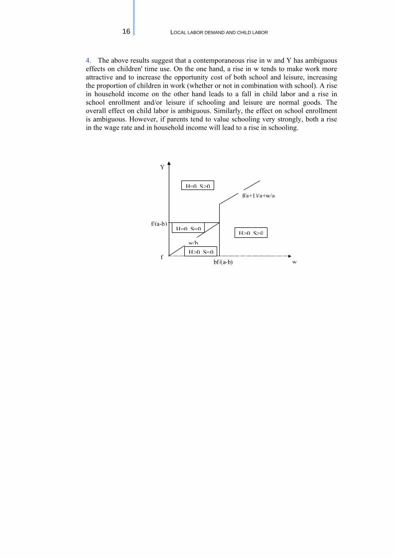
1. To understand the likely implications of a contemporaneous rise in household income and children's wages, assume that households maximize the following very simple Stone-Geary utility function: (A1) U= lnC+ aS+ bL where C is consumption, S is schooling and L is leisure. The model is extremely simplified in so far as it assumes separability of leisure and schooling. Maximization is achieved under a budget and a time constraint: (A2) C = Y + wH − fS (A3) L = 1 − H − S where Y is unearned income (including parents' ad siblings' earnings), w is the wage rate, H is work and f is the cost of schooling. The second constraint simply states that children split their time endowment (standardized to 1) into leisure, work and schooling. 2. One can solve the problem above with respect to H, S and L. We assume that a>b(b+1), i.e. that parents value their children's schooling substantially more than their leisure and for analytical tractability we assume that b>1. Finally we assume that Y>f, i.e. that household income is always sufficient to cover tuition costs. In the picture we present the equilibrium. 3. Four regimes are possible.
i. Child labor with no schooling (H>0, S=0). This arises if household income is low and wages are comparatively high. The opportunity cost of leisure (w) and schooling (w+f) are low compared to the marginal utility of consumption. Parents finance consumption through child labor.
ii. Idleness (H=0, S=0). At any given (low) wage a marginal rise in household income pushes children away from the labor market into idleness, given that leisure is a normal good. Similarly, at given low income, a marginal fall in the wage rate reduces the opportunity cost of leisure, hence increasing idleness.
iii. Schooling with no labor (H=0, S>0). Further increases in household income push children into school. Since school is more costly than leisure but also more highly valued by households, some individuals transit from inactivity to school. Others stop combining work with school and devote entirely to school.
iv. Work in combination with school (H>0, S>0). A rise in the wage rate reduces the consumption of leisure increasing labor supply. Since the opportunity cost of school increases too, some individuals transit from school only to school in combination with work. Others switch from work only to work in combination with school as the extra income accruing to working children is used to finance their schooling. Potentially the supply of labor might fall if the income effect of a rise in the wage rate prevails over the substitution effect.
16 LOCAL LABOR DEMAND AND CHILD LABOR
4. The above results suggest that a contemporaneous rise in w and Y has ambiguous effects on children' time use. On the one hand, a rise in w tends to make work more attractive and to increase the opportunity cost of both school and leisure, increasing the proportion of children in work (whether or not in combination with school). A rise in household income on the other hand leads to a fall in child labor and a rise in school enrollment and/or leisure if schooling and leisure are normal goods. The overall effect on child labor is ambiguous. Similarly, the effect on school enrollment is ambiguous. However, if parents tend to value schooling very strongly, both a rise in the wage rate and in household income will lead to a rise in schooling.
w
Y
bf/(a-b)
f/(a-b)
f
w/b
f(a+1)/a+w/a
H>0, S>0
H=0, S>0
H=0, S=0
H>0, S=0
17 UCW WORKING PAPER SERIES, MARCH 2007
REFERENCES
Basu, K. and Van, P. H. (1998), “The economics of child labor”, The American Economic Review, 88 (3), 412-27. Blanchflower D. (1999) “What can be done to reduce the high levels of youth joblessness in the world?”, mimeo, department of economics, Dartmouth College, 1999. Blanchflower, David G. and Richard B. Freeman (2000a), “Introduction”, in Blanchflower D. G. and R. B. Freeman (ed.s) “Youth Employment and Joblessness in Advanced Countries”, University of Chicago Press and NBER, 2000. Blanchflower, David G. and Richard B. Freeman (2000b), “The Declining Economic Status of Young Workers in OECD Countries”, in Blanchflower D. G. and R. B. Freeman (ed.s) “Youth Employment and Joblessness in Advanced Countries”, University of Chicago Press and NBER, 2000. Bourguignon Francois, Francisco H. G. Ferreira, and Phillippe G. Leite (2003), “Conditional Cash Transfers, Schooling, and Child Labor: Micro-Simulating Brazil's Bolsa Escola Program”, The World Bank Economic Review, Vol. 17, No. 2, 229-254 Card, David. and Thomas Lemieux (2000), “Adapting to Circumstances: The Evolution of Work, School, and Living Arrangements Among North American Youth”, in R. B. Freeman (ed.s) “Youth Employment and Joblessness in Advanced Countries”, University of Chicago Press and NBER, 2000. Cardoso Eliana and André Portela Souza (2004), “The Impact of Cash Transfers on Child Labor and School Attendance In Brazil”, Working Paper No. 04-W07, Department of Economics, Vanderbilt University, April 2004. Cigno, A and Rosati, F.C. (2005), “The economics of child labor”, Oxford University Press Duryea, Suzanne and Mary P. Arends-Kuenning (2003), “School Attendance, Child Labor and Local Labor Market Fluctuations in Urban Brazil”, World Development, 31 (7): 1165-1178. 2003. Duryea, Suzanne, David Lam and Deborah Levison (2003), “Effects of Economic Shocks on Children's Employment and Schooling in Brazil”, PSC Research Report, No. 03-541. December 2003. Eckstein Zvi and Kenneth, I. Wolpin (1999), "Why Youths Drop Out of High School: The Impact of Preferences, Opportunities, and Abilities", Econometrica, Vol. 67, No. 6 (Nov., 1999), 1295-1339.
18 LOCAL LABOR DEMAND AND CHILD LABOR
Edmonds, E. (2005) “Does Child Labor Decline with Improving Economic Status?”, The Journal of Human Resources, 40(1), Winter 2005, 77-99. Edmonds, E. (2006) “Child Labor and Schooling Responses to Anticipated Income in South Africa”, Journal of Development Economics, December 2006, 81(2), 386-414. Edmonds, E. (2007) “Child Labor”, NBER Working Papers, W12926, February 2007. Freeman, Richard B. and David A. Wise (1982), “The Youth Labor Market Problem: Its Nature, Causes, and Consequences”, in R. B. Freeman and D. A. Wise (ed.s), “The Youth Labor Market Problem: Its Nature, Causes, and Consequences”, NBER Conference Volume, University of Chicago Press and NBER, 1982. Freeman, Richard B. and William M. Rodgers III (1999), “Area Economic Conditions and the Labor Market Outcomes of Young Men in the 1990s Expansion”, NBER Working Papers, w7073, April 1999. Guarcello, Lorenzo, Marco Manacorda, Furio Rosati, Jean Fares, Scott Lyon and Cristina Valdivia (2005), “School-to-Work Transitions in Sub-Saharan Africa: An overview”, UCW Working Paper, n.15, November 2005. Guarcello, Lorenzo, Scott Lyon and Furio C. Rosati (2006), “Child Labor and Youth Employment: Ethiopia Country Study”, UCW Working Paper, July 2006. ILO (2000), “Employing Youth: Promoting Employment-Intensive Growth”, ILO, Geneva. Koreman, Sanders and David, Neumark (2000), “Cohort Crowding and Youth Labor Markets: A Cross-National Analysis”, in Blanchflower D. G. and R. B. Freeman (ed.s) “Youth Employment and Joblessness in Advanced Countries”, University of Chicago Press and NBER, 2000. Manacorda, Marco and Florence Kondylis (2006), “Youths in the Labor Market and the Transition from School to Work in Tanzania”, mimeo, Centre for Economic Performance, LSE, April 2006. Menon, M, Perali, F and Rosati, Furio C (2005), “The Shadow Wage of Child Labor: An Application to Nepal”, UCW Working paper, November 2005 OECD, (1996), “1996 Employment Outlook, Growing into work: youth and the labor market over the 1980s and 1990s” (Chapter 4), Paris, 1996. OECD, (1998), “1998 Employment Outlook, Getting started, settling in: the transition from education to the labor market” (chapter 3), Paris, 1998.
19 UCW WORKING PAPER SERIES, MARCH 2007
OECD, (1999), “Preparing Youth for the 21st Century: The Transition from Education to the Labor Market”, Paris, 1999. Parikh, Anokhi and Elisabeth Sadoulet (2005). “The Effect of Parents' Occupation on Child Labor and School Attendance in Brazil”, mimeo, University of California at Berkeley, February 2005. Udry, Christopher (2004), “Child Labor”, mimeo, department of economics, Yale University, August, 2004 Unesco (2000), “National Education for all Evaluation Report - EFA 2000”, 2000. Welch, Finis (1979) “Effects of Cohort Size on Earnings: The Baby Boom Babies Financial Bust', Journal of Political Economy, n. 87, vol. 5, 1979, S65-S97. World Bank (2001a), “Brazil. An Assessment of the Bolsa Escola Programs”, Washington DC, 2001. World Bank (2001b), “Brazil. Eradicating Child Labor in Brazil”, Washington DC, 2001 Yap Yoon-Tien, Guilherme Sedlacek
and Peter F. Orazem
(2000), “Limiting Child
Labor Through Behavior-Based Income Transfers: An Experimental Evaluation of the PETI Program in Rural Brazil”, mimeo, Inter American Development Bank, 2002.
20 LOCAL LABOR DEMAND AND CHILD LABOR
Table 1. Children's Time Use Rural Brazil - Averages over the whole sample (1) (2) (3) (4) (5) (6) (7) Age work school work & school idle work & no school school & no work hours (if work) Boys 10 0.260 0.809 0.165 0.096 0.094 0.644 28.413 11 0.341 0.804 0.221 0.077 0.119 0.582 29.399 12 0.438 0.758 0.267 0.071 0.171 0.491 31.570 13 0.533 0.690 0.289 0.065 0.245 0.402 34.455 14 0.629 0.600 0.290 0.061 0.338 0.310 37.106 15 0.719 0.494 0.271 0.058 0.448 0.223 39.808 total 0.482 0.696 0.250 0.072 0.232 0.447 34.653 Girls 10 0.086 0.836 0.063 0.140 0.023 0.773 26.483 11 0.122 0.819 0.084 0.143 0.038 0.735 28.181 12 0.175 0.773 0.106 0.158 0.069 0.667 30.648 13 0.231 0.697 0.117 0.189 0.113 0.580 33.530 14 0.290 0.611 0.126 0.224 0.164 0.485 35.665 15 0.345 0.519 0.125 0.261 0.220 0.394 37.693 Total 0.205 0.714 0.103 0.184 0.102 0.611 33.625
21 UCW WORKING PAPER SERIES, MARCH 2007Table 2 (cont.). Children's Time Use Urban Brazil - Averages over the whole sample
(1) (2) (3) (4) (5) (6) (7) Age work school work & school idle work & no school school & no work hours (if work) Boys 10 0.040 0.936 0.031 0.054 0.009 0.905 27.536 11 0.065 0.933 0.047 0.049 0.018 0.886 29.182 12 0.102 0.919 0.075 0.053 0.027 0.845 30.816 13 0.152 0.891 0.103 0.060 0.049 0.787 33.775 14 0.230 0.841 0.145 0.074 0.085 0.696 37.136 15 0.335 0.768 0.193 0.090 0.142 0.575 40.021 Total 0.153 0.882 0.098 0.063 0.055 0.783 35.919 Girls 10 0.015 0.949 0.011 0.047 0.004 0.938 31.360 11 0.030 0.944 0.022 0.048 0.008 0.922 33.525 12 0.052 0.923 0.035 0.060 0.017 0.888 36.594 13 0.088 0.892 0.054 0.074 0.034 0.838 39.524 14 0.137 0.841 0.079 0.101 0.059 0.762 41.678 15 0.200 0.771 0.108 0.137 0.092 0.662 43.260 Total 0.088 0.886 0.052 0.078 0.036 0.834 40.696
The table reports information on time use patterns of children aged 10-15 in urban and rural Brazil. Column (1) reports the proportion in work, column (2) the proportion in school, column (3) the proportion combining work and school, column (4) the proportion neither in school nor in work, column (5) the proportion working and not attending school (full time work) and column (6) the proportion in school and not in work (full time school). Column (7) reports average working hours among working children. The top part of the table refers to boys and the bottom part to girls Number of observations in urban areas: 332,045 for boys and 324,425 for girls. Number of observations in rural areas: 107,335 for boys and 99,108 for girls. Source PNAD individual records: 1981-2002.
22 LOCAL LABOR DEMAND AND CHILD LABOR
Table 2. Local labor Demand and Children's Time use - No controls (1) (2) (3) (4) (5) (6) (7) (8) (9) work school work & school idle work & no school school & no work weekly work hours log household income log wages RURAL Males 0.956*** 0.106 0.685*** -0.379*** 0.270** -0.576*** 27.292*** -0.418 1.483* (0.181) (0.152) (0.163) (0.093) (0.131) (0.168) (6.443) (0.538) (0.755) Females 0.446*** 0.077 0.404*** -0.115 0.043 -0.332** 11.629*** 0.404 1.333 (0.134) (0.130) (0.114) (0.117) (0.069) (0.158) (3.798) (0.508) (1.166) URBAN Males 0.233*** 0.078 0.181*** -0.129** 0.053 -0.104 5.368* 2.186*** 2.002*** (0.086) (0.067) (0.069) (0.051) (0.051) (0.087) (3.047) (0.370) (0.509) Females -0.028 0.018 0.007 0.014 -0.033 0.012 -4.471* 1.988*** 3.283*** (0.057) (0.062) (0.047) (0.049) (0.032) (0.073) (2.423) (0.368) (0.763)
The table reports results of an OLS regression of each variable (in the top row) on the employment to population ratio of individuals aged 25-50 in the area or residence (rural or urban part of each state) and year (equation 1). All regressions control for state, year and age effects and interactions of decade dummies (1980s, 1990s and 2000s) with state dummies. Standard errors clustered by state and year.
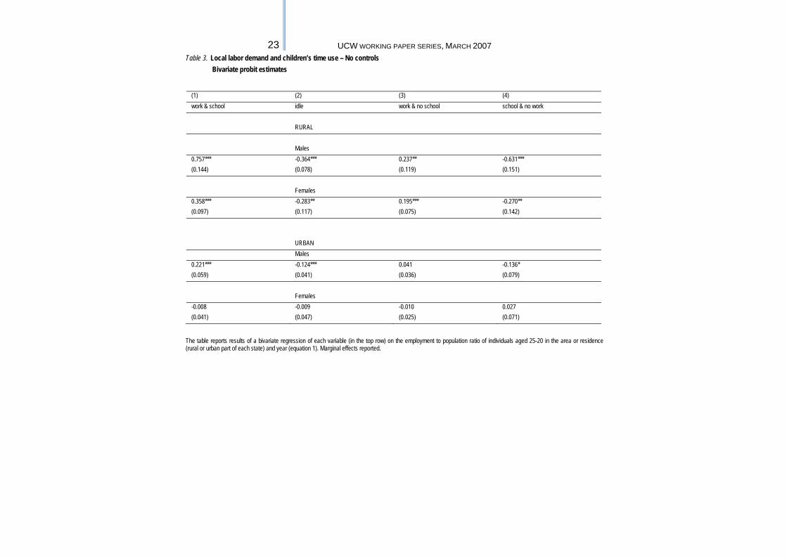
23 UCW WORKING PAPER SERIES, MARCH 2007Table 3. Local labor demand and children’s time use – No controls
Bivariate probit estimates
(1) (2) (3) (4) work & school idle work & no school school & no work RURAL Males 0.757*** -0.364*** 0.237** -0.631*** (0.144) (0.078) (0.119) (0.151) Females 0.358*** -0.283** 0.195*** -0.270** (0.097) (0.117) (0.075) (0.142) URBAN Males 0.221*** -0.124*** 0.041 -0.136* (0.059) (0.041) (0.036) (0.079) Females -0.008 -0.009 -0.010 0.027 (0.041) (0.047) (0.025) (0.071)
The table reports results of a bivariate regression of each variable (in the top row) on the employment to population ratio of individuals aged 25-20 in the area or residence (rural or urban part of each state) and year (equation 1). Marginal effects reported.
24 LOCAL LABOR DEMAND AND CHILD LABOR
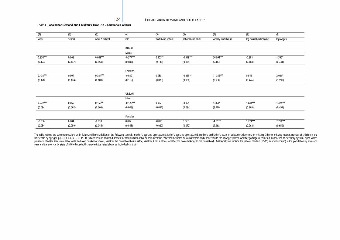
Table 4. Local labor Demand and Children's Time use - Additional Controls
(1) (2) (3) (4) (5) (6) (7) (8) (9) work school work & school idle work & no school school & no work weekly work hours log household income log wages RURAL Males 0.958*** 0.068 0.649*** -0.377*** 0.307** -0.579*** 26.991*** -0.281 1.356* (0.174) (0.147) (0.158) (0.087) (0.133) (0.159) (6.183) (0.483) (0.731) Females 0.435*** 0.004 0.354*** -0.080 0.080 -0.355** 11.355*** 0.545 2.031* (0.128) (0.124) (0.109) (0.115) (0.073) (0.150) (3.730) (0.446) (1.193) URBAN Males 0.222*** 0.065 0.159** -0.126*** 0.062 -0.095 5.064* 1.844*** 1.474*** (0.084) (0.062) (0.066) (0.048) (0.051) (0.084) (2.960) (0.265) (0.499) Females -0.036 0.004 -0.018 0.012 -0.016 0.022 -4.097* 1.721*** 2.711*** (0.054) (0.059) (0.045) (0.046) (0.030) (0.072) (2.268) (0.263) (0.659)
The table reports the same regressions as in Table 2 with the addition of the following controls: mother's age and age squared, father's age and age squared, mother's and father's years of education, dummies for missing father or missing mother, number of children in the household by age group (0, 1-3, 4-6, 7-9, 10-15, 16-18 and 19 and above) dummies for total number of household members, whether the home has a bathroom and connection to the sewage system, whether garbage is collected, connection to electricity system, piped water, presence of water filter, material of walls and roof, number of rooms, whether the household has a fridge, whether it has a stove, whether the home belongs to the household). Additionally we include the ratio of children (10-15) to adults (25-50) in the population by state and year and the average by state of all the household characteristics listed above as individual controls.
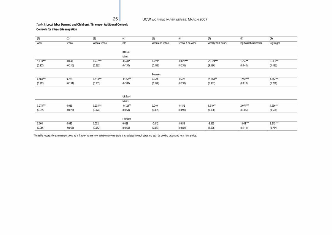
25 UCW WORKING PAPER SERIES, MARCH 2007Table 5. Local labor Demand and Children's Time use - Additional Controls Controls for intra-state migration
(1) (2) (3) (4) (5) (6) (7) (8) (9) work school work & school idle work & no school school & no work weekly work hours log household income log wages RURAL Males 1.074*** -0.047 0.772*** -0.249* 0.299* -0.822*** 25.324*** 1.259** 5.003*** (0.255) (0.216) (0.233) (0.130) (0.179) (0.235) (9.586) (0.640) (1.133) Females 0.584*** 0.289 0.514*** -0.357** 0.070 -0.227 15.464** 1.966*** 4.582*** (0.203) (0.194) (0.155) (0.180) (0.120) (0.232) (6.137) (0.610) (1.288) URBAN Males 0.275*** 0.083 0.235*** -0.123** 0.040 -0.152 6.619** 2.074*** 1.936*** (0.095) (0.072) (0.074) (0.053) (0.055) (0.098) (3.338) (0.306) (0.568) Females 0.008 0.015 0.052 0.028 -0.042 -0.038 -3.363 1.941*** 3.513*** (0.065) (0.066) (0.052) (0.050) (0.033) (0.084) (2.596) (0.311) (0.734)
The table reports the same regressions as in Table 4 where now adult employment rate is calculated in each state and year by pooling urban and rural households.
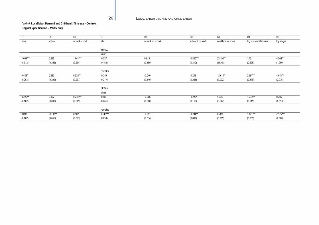
26 LOCAL LABOR DEMAND AND CHILD LABOR
Table 6. Local labor Demand and Children's Time use - Controls Original Specification – 1990S only (1) (2) (3) (4) (5) (6) (7) (8) (9) work school work & school idle work & no school school & no work weekly work hours log household income log wages RURAL Males 1.059*** 0.215 1.041*** -0.227 0.015 -0.830*** 23.190** 1.131 4.564*** (0.312) (0.242) (0.294) (0.152) (0.189) (0.310) (10.403) (0.805) (1.250) Females 0.485* 0.290 0.524** -0.245 -0.040 -0.239 12.614* 2.697*** 4.681** (0.253) (0.229) (0.207) (0.217) (0.140) (0.263) (7.002) (0.670) (2.075) URBAN Males 0.225** 0.002 0.231*** 0.003 -0.006 -0.228* 5.745 1.272*** 0.205 (0.107) (0.088) (0.089) (0.061) (0.060) (0.118) (3.642) (0.319) (0.693) Females 0.092 -0.138** 0.107 0.148*** -0.011 -0.244** 0.789 1.121*** 2.575*** (0.087) (0.065) (0.073) (0.053) (0.034) (0.099) (3.205) (0.339) (0.880)

27 UCW WORKING PAPER SERIES, MARCH 2007Table 7. Local labor Demand and Children's Time use - Controls Controlling for intra- and inter-state migration- – 1990s only (1) (2) (3) (4) (5) (6) (7) (8) (9) work school work & school idle work & no school school & no work weekly work hours log household income log wages RURAL Males 1.231*** 0.153 1.142*** -0.231 0.085 -0.996*** 30.487*** 1.138 3.318** (0.300) (0.254) (0.280) (0.157) (0.181) (0.311) (9.968) (0.776) (1.290) Females 0.634*** 0.302 0.696*** -0.235 -0.063 -0.399* 16.952** 2.390*** 1.337 (0.221) (0.220) (0.186) (0.215) (0.117) (0.226) (6.794) (0.748) (1.814) URBAN Males 0.189* 0.004 0.219** 0.027 -0.030 -0.216* 6.240* 1.073*** 1.083 (0.109) (0.089) (0.093) (0.066) (0.059) (0.115) (3.759) (0.278) (0.700) Females 0.152* -0.144** 0.143** 0.129** 0.013 -0.285*** 3.548 0.917*** -0.342 (0.085) (0.073) (0.071) (0.063) (0.033) (0.109) (3.017) (0.317) (1.026) The top of the table reports the same regressions as in Table 5 estimated only on the period 1990-2002. The tables re-imputes children back to their (or their parents') state of birth (as opposed to their state of residence). See text for details.
28 LOCAL LABOR DEMAND AND CHILD LABOR
Table 8. Local labor Demand and Children's Time use - Controls Separately by household income (1) (2) (3) (4) (5) (6) (7) (8) (9) work school work & school idle work & no school school & no work weekly work hours log household income log wages RURAL Males low 1.205*** -0.163 0.798*** -0.237* 0.405** -0.966*** 28.352*** 2.228*** 5.774*** (0.274) (0.214) (0.236) (0.137) (0.185) (0.251) (10.518) (0.702) (1.322) middle 1.195*** -0.169 0.806*** -0.213 0.385** -0.979*** 29.577*** 1.575** 5.344*** (0.272) (0.213) (0.231) (0.132) (0.190) (0.245) (10.545) (0.650) (1.182) high 0.644** 0.183 0.626*** -0.196 0.016 -0.446* 8.222 1.672*** 4.657*** (0.267) (0.225) (0.237) (0.139) (0.191) (0.256) (10.309) (0.638) (1.191) Females low 0.636*** 0.280 0.550*** -0.364* 0.085 -0.272 16.971*** 2.799*** 4.048*** (0.203) (0.210) (0.166) (0.186) (0.124) (0.246) (6.421) (0.685) (1.358) middle 0.574*** 0.366* 0.471*** -0.467** 0.103 -0.107 14.682** 1.878*** 3.490*** (0.208) (0.206) (0.166) (0.195) (0.118) (0.255) (6.433) (0.604) (1.275) high 0.311 0.545*** 0.453*** -0.401** -0.142 0.090 5.157 2.141*** 5.008*** (0.213) (0.203) (0.163) (0.184) (0.127) (0.257) (6.761) (0.603) (1.396) URBAN Males low 0.557*** -0.118 0.270*** -0.169*** 0.286*** -0.387*** 20.990*** 2.805*** 2.015*** (0.101) (0.088) (0.082) (0.064) (0.063) (0.113) (3.561) (0.318) (0.599) middle 0.273*** 0.023 0.222*** -0.074 0.050 -0.198* 6.734* 2.020*** 2.510*** (0.098) (0.073) (0.081) (0.053) (0.056) (0.104) (3.432) (0.301) (0.614) high -0.050 0.332*** 0.184** -0.099* -0.233*** 0.149 -10.718*** 1.226*** 2.281*** (0.098) (0.079) (0.078) (0.054) (0.058) (0.106) (3.460) (0.317) (0.675) Females low 0.292*** -0.263*** 0.151*** 0.121* 0.142*** -0.414*** 9.087*** 2.722*** 3.107*** (0.077) (0.084) (0.058) (0.062) (0.043) (0.104) (3.211) (0.328) (0.764) middle 0.013 0.018 0.056 0.024 -0.041 -0.039 -3.409 2.014*** 4.302*** (0.068) (0.072) (0.057) (0.057) (0.034) (0.089) (2.676) (0.313) (0.784) high -0.287*** 0.315*** -0.072 -0.100* -0.213*** 0.386*** -16.926*** 1.259*** 3.977*** (0.070) (0.078) (0.057) (0.059) (0.038) (0.093) (2.844) (0.329) (0.904) The table reports the same regressions as in Table 4 where we allow the coefficient on local labor demand to vary according to the household position in the distribution of income in its area of residence.
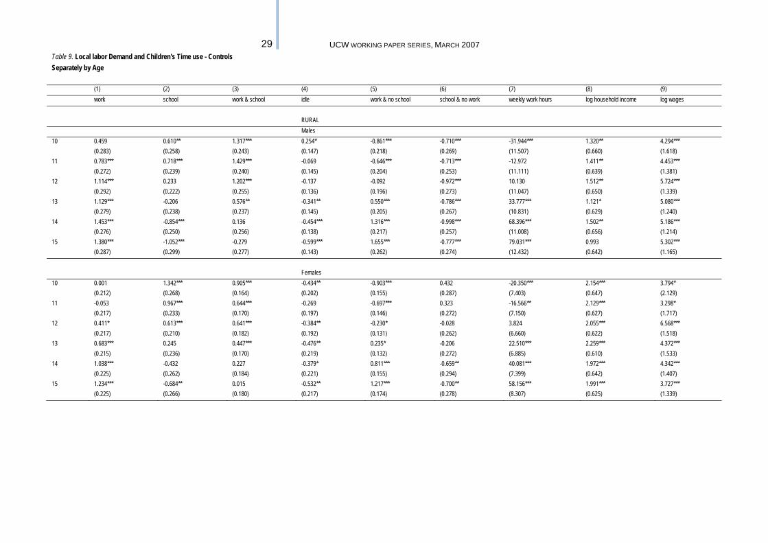
29 UCW WORKING PAPER SERIES, MARCH 2007Table 9. Local labor Demand and Children's Time use - Controls Separately by Age (1) (2) (3) (4) (5) (6) (7) (8) (9) work school work & school idle work & no school school & no work weekly work hours log household income log wages RURAL Males 10 0.459 0.610** 1.317*** 0.254* -0.861*** -0.710*** -31.944*** 1.320** 4.294*** (0.283) (0.258) (0.243) (0.147) (0.218) (0.269) (11.507) (0.660) (1.618) 11 0.783*** 0.718*** 1.429*** -0.069 -0.646*** -0.713*** -12.972 1.411** 4.453*** (0.272) (0.239) (0.240) (0.145) (0.204) (0.253) (11.111) (0.639) (1.381) 12 1.114*** 0.233 1.202*** -0.137 -0.092 -0.972*** 10.130 1.512** 5.724*** (0.292) (0.222) (0.255) (0.136) (0.196) (0.273) (11.047) (0.650) (1.339) 13 1.129*** -0.206 0.576** -0.341** 0.550*** -0.786*** 33.777*** 1.121* 5.080*** (0.279) (0.238) (0.237) (0.145) (0.205) (0.267) (10.831) (0.629) (1.240) 14 1.453*** -0.854*** 0.136 -0.454*** 1.316*** -0.998*** 68.396*** 1.502** 5.186*** (0.276) (0.250) (0.256) (0.138) (0.217) (0.257) (11.008) (0.656) (1.214) 15 1.380*** -1.052*** -0.279 -0.599*** 1.655*** -0.777*** 79.031*** 0.993 5.302*** (0.287) (0.299) (0.277) (0.143) (0.262) (0.274) (12.432) (0.642) (1.165) Females 10 0.001 1.342*** 0.905*** -0.434** -0.903*** 0.432 -20.350*** 2.154*** 3.794* (0.212) (0.268) (0.164) (0.202) (0.155) (0.287) (7.403) (0.647) (2.129) 11 -0.053 0.967*** 0.644*** -0.269 -0.697*** 0.323 -16.566** 2.129*** 3.298* (0.217) (0.233) (0.170) (0.197) (0.146) (0.272) (7.150) (0.627) (1.717) 12 0.411* 0.613*** 0.641*** -0.384** -0.230* -0.028 3.824 2.055*** 6.568*** (0.217) (0.210) (0.182) (0.192) (0.131) (0.262) (6.660) (0.622) (1.518) 13 0.683*** 0.245 0.447*** -0.476** 0.235* -0.206 22.510*** 2.259*** 4.372*** (0.215) (0.236) (0.170) (0.219) (0.132) (0.272) (6.885) (0.610) (1.533) 14 1.038*** -0.432 0.227 -0.379* 0.811*** -0.659** 40.081*** 1.972*** 4.342*** (0.225) (0.262) (0.184) (0.221) (0.155) (0.294) (7.399) (0.642) (1.407) 15 1.234*** -0.684** 0.015 -0.532** 1.217*** -0.700** 58.156*** 1.991*** 3.727*** (0.225) (0.266) (0.180) (0.217) (0.174) (0.278) (8.307) (0.625) (1.339)
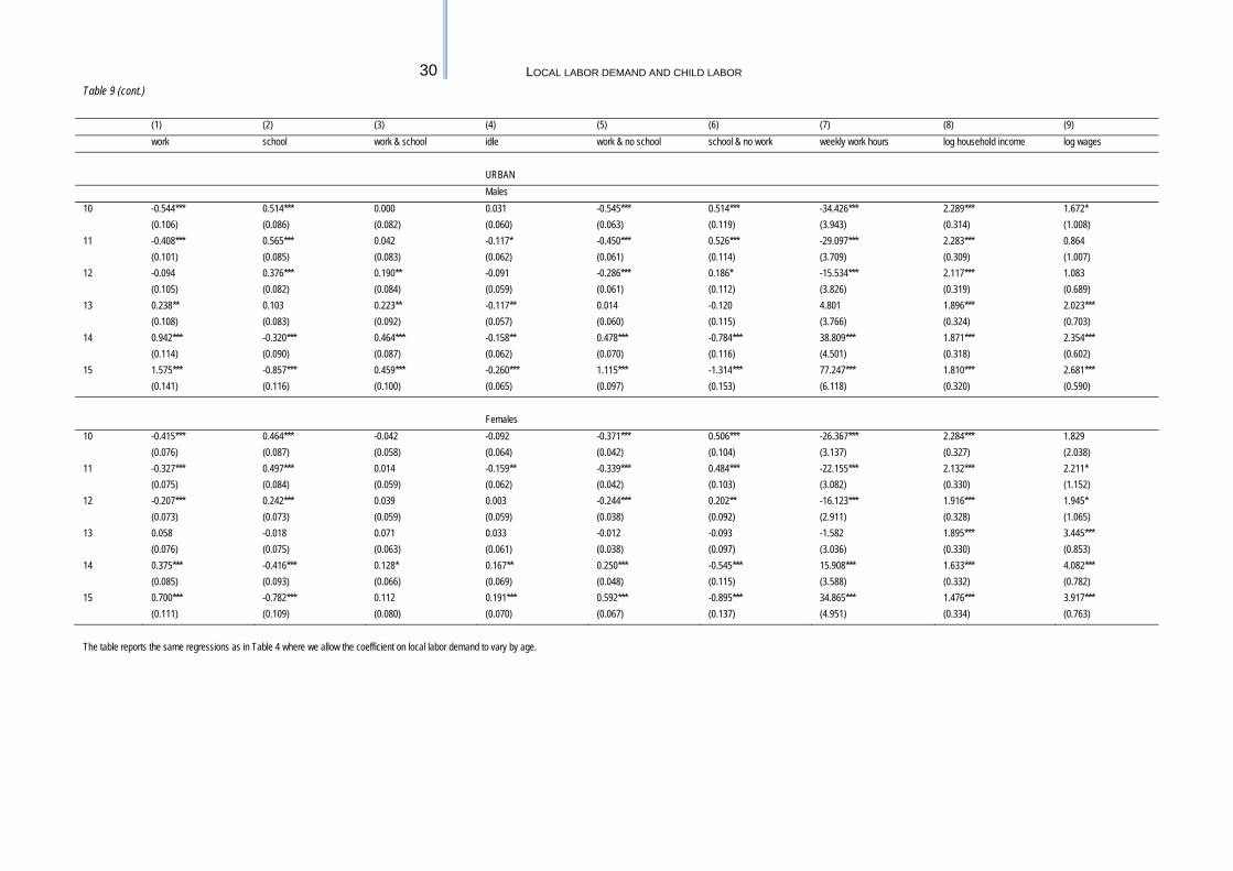
30 LOCAL LABOR DEMAND AND CHILD LABOR
Table 9 (cont.) (1) (2) (3) (4) (5) (6) (7) (8) (9) work school work & school idle work & no school school & no work weekly work hours log household income log wages URBAN Males 10 -0.544*** 0.514*** 0.000 0.031 -0.545*** 0.514*** -34.426*** 2.289*** 1.672* (0.106) (0.086) (0.082) (0.060) (0.063) (0.119) (3.943) (0.314) (1.008) 11 -0.408*** 0.565*** 0.042 -0.117* -0.450*** 0.526*** -29.097*** 2.283*** 0.864 (0.101) (0.085) (0.083) (0.062) (0.061) (0.114) (3.709) (0.309) (1.007) 12 -0.094 0.376*** 0.190** -0.091 -0.286*** 0.186* -15.534*** 2.117*** 1.083 (0.105) (0.082) (0.084) (0.059) (0.061) (0.112) (3.826) (0.319) (0.689) 13 0.238** 0.103 0.223** -0.117** 0.014 -0.120 4.801 1.896*** 2.023*** (0.108) (0.083) (0.092) (0.057) (0.060) (0.115) (3.766) (0.324) (0.703) 14 0.942*** -0.320*** 0.464*** -0.158** 0.478*** -0.784*** 38.809*** 1.871*** 2.354*** (0.114) (0.090) (0.087) (0.062) (0.070) (0.116) (4.501) (0.318) (0.602) 15 1.575*** -0.857*** 0.459*** -0.260*** 1.115*** -1.314*** 77.247*** 1.810*** 2.681*** (0.141) (0.116) (0.100) (0.065) (0.097) (0.153) (6.118) (0.320) (0.590) Females 10 -0.415*** 0.464*** -0.042 -0.092 -0.371*** 0.506*** -26.367*** 2.284*** 1.829 (0.076) (0.087) (0.058) (0.064) (0.042) (0.104) (3.137) (0.327) (2.038) 11 -0.327*** 0.497*** 0.014 -0.159** -0.339*** 0.484*** -22.155*** 2.132*** 2.211* (0.075) (0.084) (0.059) (0.062) (0.042) (0.103) (3.082) (0.330) (1.152) 12 -0.207*** 0.242*** 0.039 0.003 -0.244*** 0.202** -16.123*** 1.916*** 1.945* (0.073) (0.073) (0.059) (0.059) (0.038) (0.092) (2.911) (0.328) (1.065) 13 0.058 -0.018 0.071 0.033 -0.012 -0.093 -1.582 1.895*** 3.445*** (0.076) (0.075) (0.063) (0.061) (0.038) (0.097) (3.036) (0.330) (0.853) 14 0.375*** -0.416*** 0.128* 0.167** 0.250*** -0.545*** 15.908*** 1.633*** 4.082*** (0.085) (0.093) (0.066) (0.069) (0.048) (0.115) (3.588) (0.332) (0.782) 15 0.700*** -0.782*** 0.112 0.191*** 0.592*** -0.895*** 34.865*** 1.476*** 3.917*** (0.111) (0.109) (0.080) (0.070) (0.067) (0.137) (4.951) (0.334) (0.763) The table reports the same regressions as in Table 4 where we allow the coefficient on local labor demand to vary by age.
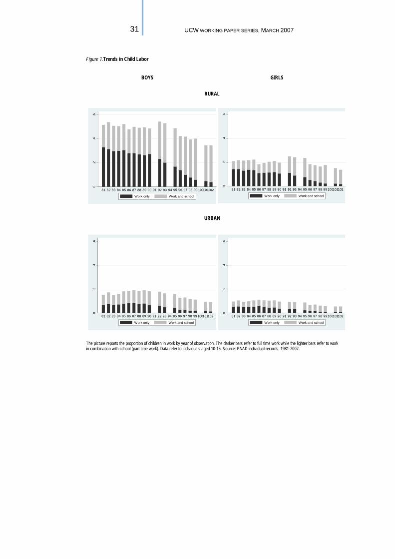
31 UCW WORKING PAPER SERIES, MARCH 2007
Figure 1.Trends in Child Labor
BOYS GIRLS
RURAL
URBAN
The picture reports the proportion of children in work by year of observation. The darker bars refer to full time work while the lighter bars refer to work in combination with school (part time work). Data refer to individuals aged 10-15. Source: PNAD individual records: 1981-2002.
0.2
.4.6
81 82 83 84 85 86 87 88 89 90 91 92 93 94 95 96 97 98 99100101102
Work only Work and school
0.2
.4.6
81 82 83 84 85 86 87 88 89 90 91 92 93 94 95 96 97 98 99100101102
Work only Work and school
0.2
.4.6
81 82 83 84 85 86 87 88 89 90 91 92 93 94 95 96 97 98 99100101102
Work only Work and school
0.2
.4.6
81 82 83 84 85 86 87 88 89 90 91 92 93 94 95 96 97 98 99100101102
Work only Work and school
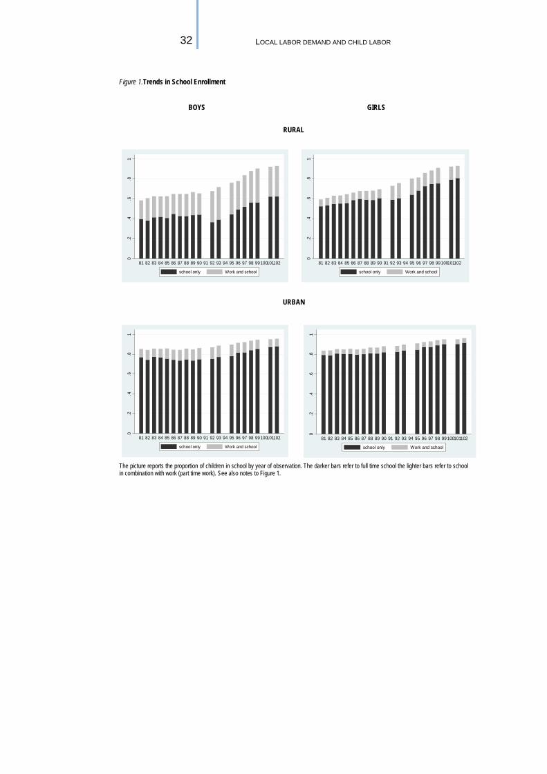
32 LOCAL LABOR DEMAND AND CHILD LABOR
Figure 1.Trends in School Enrollment
BOYS GIRLS
RURAL
URBAN
The picture reports the proportion of children in school by year of observation. The darker bars refer to full time school the lighter bars refer to school in combination with work (part time work). See also notes to Figure 1.
0.2
.4.6
.81
81 82 83 84 85 86 87 88 89 90 91 92 93 94 95 96 97 98 99100101102
school only Work and school
0.2
.4.6
.81
81 82 83 84 85 86 87 88 89 90 91 92 93 94 95 96 97 98 99 100101102
school only Work and school
0.2
.4.6
.81
81 82 83 84 85 86 87 88 89 90 91 92 93 94 95 96 97 98 99100101102
school only Work and school
0.2
.4.6
.81
81 82 83 84 85 86 87 88 89 90 91 92 93 94 95 96 97 98 99100101102
school only Work and school
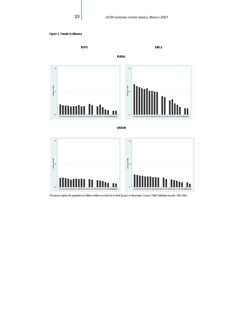
33 UCW WORKING PAPER SERIES, MARCH 2007
Figure 3. Trends in idleness
BOYS GIRLS
RURAL
URBAN
The picture reports the proportion of children neither in school nor in work by year of observation. Source: PNAD individual records: 1981-2002.
0.2
.4m
ean
of id
le
81 82 83 84 85 86 87 88 89 90 91 92 93 94 95 96 97 98 99100101102
0.2
.4m
ean
of id
le
81 82 83 84 85 86 87 88 89 90 91 92 93 94 95 96 97 98 99100101102
0.2
.4m
ean
of id
le
81 82 83 84 85 86 87 88 89 90 91 92 93 94 95 96 97 98 99100101102
0.2
.4m
ean
of id
le
81 82 83 84 85 86 87 88 89 90 91 92 93 94 95 96 97 98 99100101102
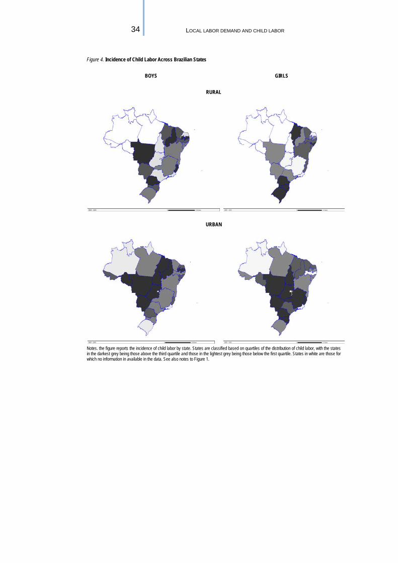
34 LOCAL LABOR DEMAND AND CHILD LABOR
Figure 4. Incidence of Child Labor Across Brazilian States
BOYS GIRLS
RURAL
URBAN
Notes. the figure reports the incidence of child labor by state. States are classified based on quartiles of the distribution of child labor, with the states in the darkest grey being those above the third quartile and those in the lightest grey being those below the first quartile. States in white are those for which no information in available in the data. See also notes to Figure 1.
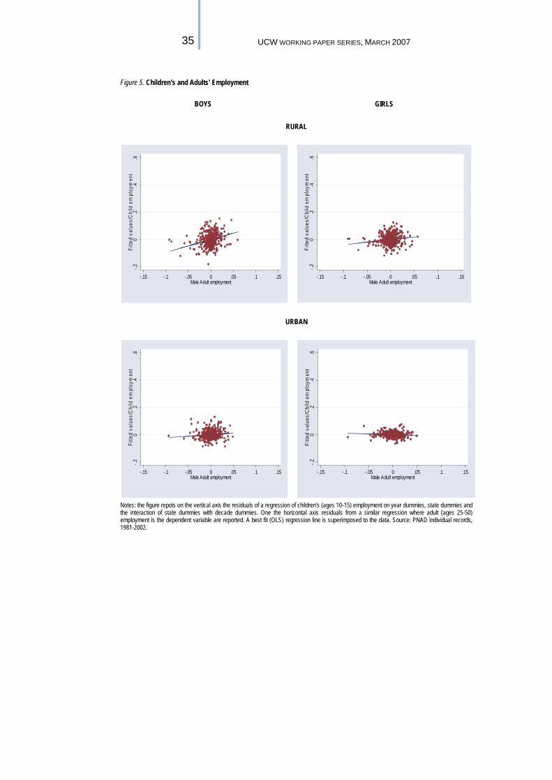
35 UCW WORKING PAPER SERIES, MARCH 2007
Figure 5. Children's and Adults' Employment
BOYS GIRLS
RURAL
URBAN
Notes: the figure repots on the vertical axis the residuals of a regression of children's (ages 10-15) employment on year dummies, state dummies and the interaction of state dummies with decade dummies. One the horizontal axis residuals from a similar regression where adult (ages 25-50) employment is the dependent variable are reported. A best fit (OLS) regression line is superimposed to the data. Source: PNAD individual records, 1981-2002.
-.20
.2.4
.6Fi
tted
valu
es/C
hild
em
ploy
men
t
-.15 -.1 -.05 0 .05 .1 .15Male Adult employment
-.20
.2.4
.6Fi
tted
valu
es/C
hild
em
ploy
men
t
-.15 -.1 -.05 0 .05 .1 .15Male Adult employment
-.20
.2.4
.6Fi
tted
valu
es/C
hild
em
ploy
men
t
-.15 -.1 -.05 0 .05 .1 .15Male Adult employment
-.20
.2.4
.6Fi
tted
valu
es/C
hild
em
ploy
men
t
-.15 -.1 -.05 0 .05 .1 .15Male Adult employment
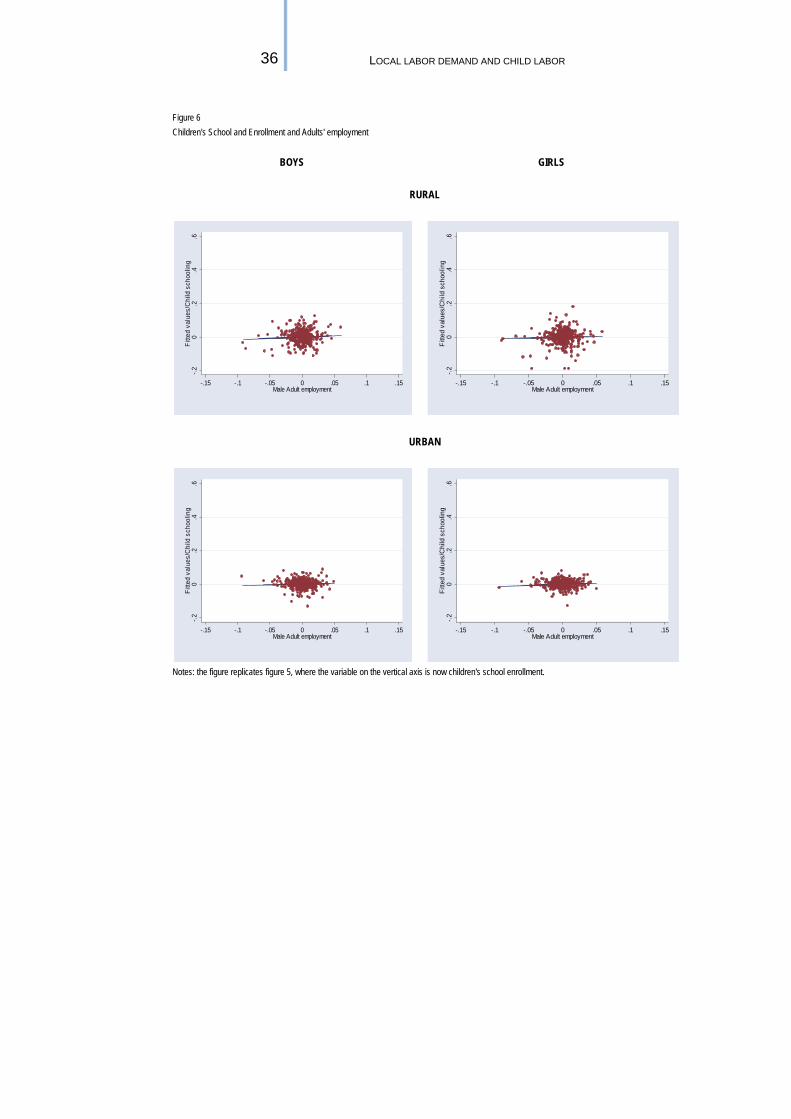
36 LOCAL LABOR DEMAND AND CHILD LABOR
Figure 6 Children's School and Enrollment and Adults' employment
BOYS GIRLS
RURAL
URBAN
Notes: the figure replicates figure 5, where the variable on the vertical axis is now children's school enrollment.
-.20
.2.4
.6Fi
tted
valu
es/C
hild
sch
oolin
g
-.15 -.1 -.05 0 .05 .1 .15Male Adult employment
-.20
.2.4
.6Fi
tted
valu
es/C
hild
sch
oolin
g
-.15 -.1 -.05 0 .05 .1 .15Male Adult employment
-.20
.2.4
.6Fi
tted
valu
es/C
hild
sch
oolin
g
-.15 -.1 -.05 0 .05 .1 .15Male Adult employment
-.20
.2.4
.6Fi
tted
valu
es/C
hild
sch
oolin
g
-.15 -.1 -.05 0 .05 .1 .15Male Adult employment
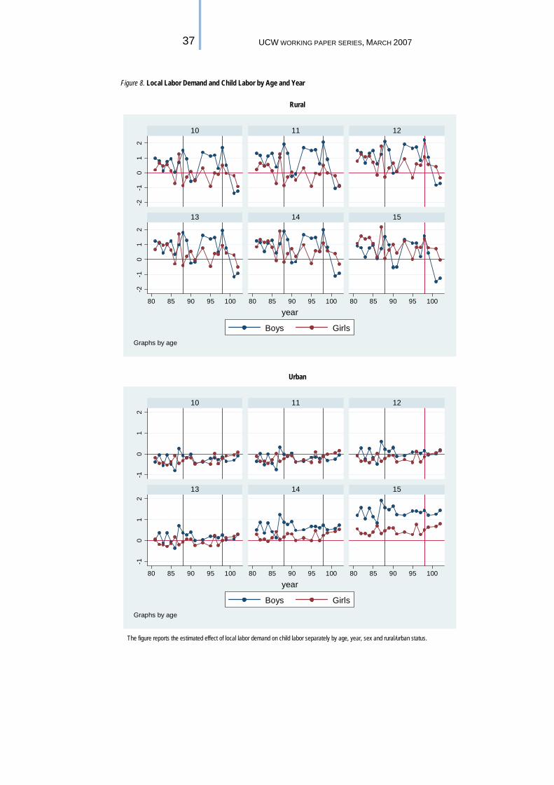
37 UCW WORKING PAPER SERIES, MARCH 2007
Figure 8. Local Labor Demand and Child Labor by Age and Year
Rural
Urban
The figure reports the estimated effect of local labor demand on child labor separately by age, year, sex and rural/urban status.
-2-1
01
2-2
-10
12
80 85 90 95 100 80 85 90 95 100 80 85 90 95 100
10 11 12
13 14 15
Boys Girls
year
Graphs by age
-10
12
-10
12
80 85 90 95 100 80 85 90 95 100 80 85 90 95 100
10 11 12
13 14 15
Boys Girls
year
Graphs by age