Stabilizing Cell Phone Video using Inertial Measurement Sensors

Gustav Hanning, Nicklas Forslow, Per-Erik Forssen, Erik Ringaby, David Tornqvist, Jonas Callmer

Department of Electrical Engineering

Linkoping University

http://www.liu.se/forskning/foass/per-erik-forssen/VGS

Abstract

We present a system that rectifies and stabilizes video

sequences on mobile devices with rolling-shutter cameras.

The system corrects for rolling-shutter distortions using

measurements from accelerometer and gyroscope sensors,

and a 3D rotational distortion model. In order to obtain

a stabilized video, and at the same time keep most content

in view, we propose an adaptive low-pass filter algorithm

to obtain the output camera trajectory. The accuracy of the

orientation estimates has been evaluated experimentally us-

ing ground truth data from a motion capture system. We

have conducted a user study, where the output from our sys-

tem, implemented in iOS, has been compared to that of three

other applications, as well as to the uncorrected video. The

study shows that users prefer our sensor-based system.

1. Introduction

Most mobile video-recording devices of today make use

of CMOS sensors with rolling-shutter (RS) readout [6]. An

RS camera captures video by exposing every frame line-by-

line from top to bottom. This is in contrast to a global shut-

ter, where an entire frame is acquired at once.

The RS technique gives rise to image distortions in sit-

uations where either the device or the target is moving.

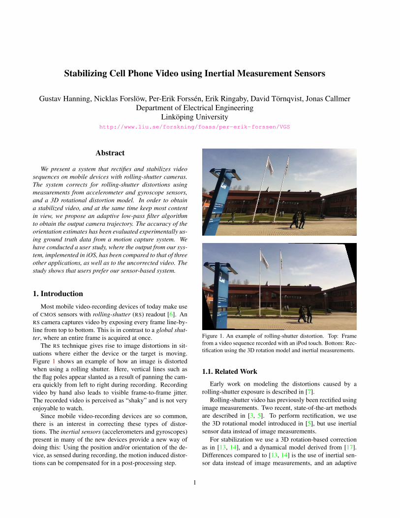
Figure 1 shows an example of how an image is distorted

when using a rolling shutter. Here, vertical lines such as

the flag poles appear slanted as a result of panning the cam-

era quickly from left to right during recording. Recording

video by hand also leads to visible frame-to-frame jitter.

The recorded video is perceived as “shaky” and is not very

enjoyable to watch.

Since mobile video-recording devices are so common,

there is an interest in correcting these types of distor-

tions. The inertial sensors (accelerometers and gyroscopes)

present in many of the new devices provide a new way of

doing this: Using the position and/or orientation of the de-

vice, as sensed during recording, the motion induced distor-

tions can be compensated for in a post-processing step.

Figure 1. An example of rolling-shutter distortion. Top: Frame

from a video sequence recorded with an iPod touch. Bottom: Rec-

tification using the 3D rotation model and inertial measurements.

1.1. Related Work

Early work on modeling the distortions caused by a

rolling-shutter exposure is described in [7].

Rolling-shutter video has previously been rectified using

image measurements. Two recent, state-of-the-art methods

are described in [3, 5]. To perform rectification, we use

the 3D rotational model introduced in [5], but use inertial

sensor data instead of image measurements.

For stabilization we use a 3D rotation-based correction

as in [13, 14], and a dynamical model derived from [17].

Differences compared to [13, 14] is the use of inertial sen-

sor data instead of image measurements, and an adaptive

1

SynchronizationCamera

Gyroscope

Accelerometer

EKF & EKFS

CUSUM LS �lterAdaptive

low-pass �lter

Stabilization &

Recti�cation

Resulting video

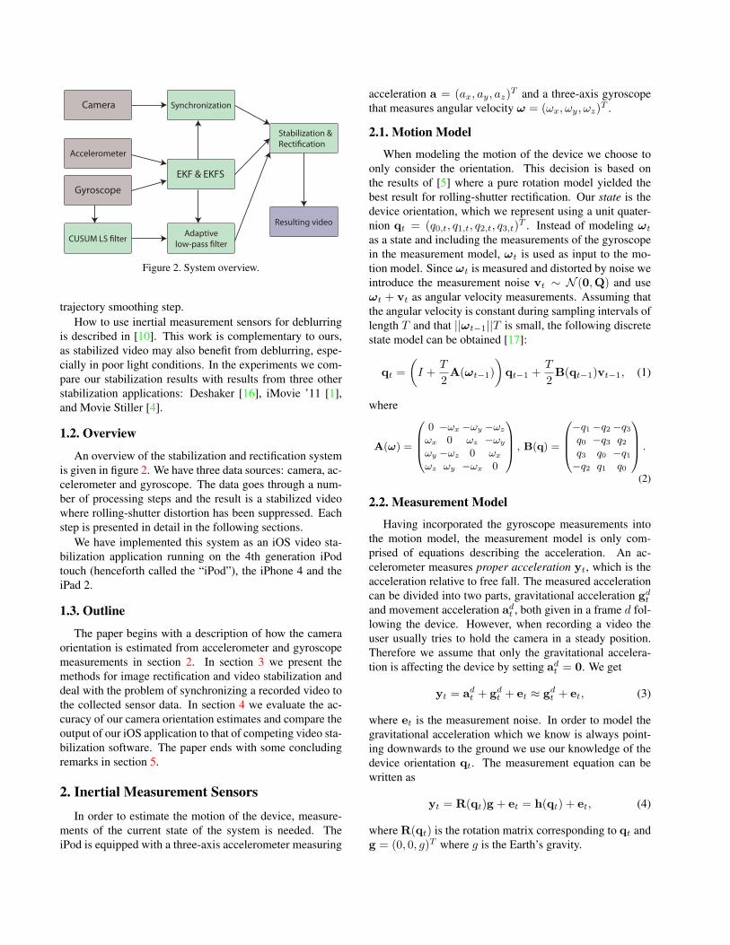
Figure 2. System overview.

trajectory smoothing step.

How to use inertial measurement sensors for deblurring

is described in [10]. This work is complementary to ours,

as stabilized video may also benefit from deblurring, espe-

cially in poor light conditions. In the experiments we com-

pare our stabilization results with results from three other

stabilization applications: Deshaker [16], iMovie ’11 [1],

and Movie Stiller [4].

1.2. Overview

An overview of the stabilization and rectification system

is given in figure 2. We have three data sources: camera, ac-

celerometer and gyroscope. The data goes through a num-

ber of processing steps and the result is a stabilized video

where rolling-shutter distortion has been suppressed. Each

step is presented in detail in the following sections.

We have implemented this system as an iOS video sta-

bilization application running on the 4th generation iPod

touch (henceforth called the “iPod”), the iPhone 4 and the

iPad 2.

1.3. Outline

The paper begins with a description of how the camera

orientation is estimated from accelerometer and gyroscope

measurements in section 2. In section 3 we present the

methods for image rectification and video stabilization and

deal with the problem of synchronizing a recorded video to

the collected sensor data. In section 4 we evaluate the ac-

curacy of our camera orientation estimates and compare the

output of our iOS application to that of competing video sta-

bilization software. The paper ends with some concluding

remarks in section 5.

2. Inertial Measurement Sensors

In order to estimate the motion of the device, measure-

ments of the current state of the system is needed. The

iPod is equipped with a three-axis accelerometer measuring

acceleration a = (ax, ay, az)T and a three-axis gyroscope

that measures angular velocity ω = (ωx, ωy, ωz)T .

2.1. Motion Model

When modeling the motion of the device we choose to

only consider the orientation. This decision is based on

the results of [5] where a pure rotation model yielded the

best result for rolling-shutter rectification. Our state is the

device orientation, which we represent using a unit quater-

nion qt = (q0,t, q1,t, q2,t, q3,t)T . Instead of modeling ωt

as a state and including the measurements of the gyroscope

in the measurement model, ωt is used as input to the mo-

tion model. Since ωt is measured and distorted by noise we

introduce the measurement noise vt ∼ N (0,Q) and use

ωt + vt as angular velocity measurements. Assuming that

the angular velocity is constant during sampling intervals of

length T and that ||ωt−1||T is small, the following discrete

state model can be obtained [17]:

qt =

(

I +T

2A(ωt−1)

)

qt−1 +T

2B(qt−1)vt−1, (1)

where

A(ω) =

0

B

B

@

0 −ωx−ωy −ωz

ωx 0 ωz −ωy

ωy −ωz 0 ωx

ωz ωy −ωx 0

1

C

C

A

, B(q) =

0

B

B

@

−q1−q2−q3q0 −q3 q2q3 q0 −q1−q2 q1 q0

1

C

C

A

.

(2)

2.2. Measurement Model

Having incorporated the gyroscope measurements into

the motion model, the measurement model is only com-

prised of equations describing the acceleration. An ac-

celerometer measures proper acceleration yt, which is the

acceleration relative to free fall. The measured acceleration

can be divided into two parts, gravitational acceleration gdt

and movement acceleration adt , both given in a frame d fol-

lowing the device. However, when recording a video the

user usually tries to hold the camera in a steady position.

Therefore we assume that only the gravitational accelera-

tion is affecting the device by setting adt = 0. We get

yt = adt + gd

t + et ≈ gdt + et, (3)

where et is the measurement noise. In order to model the

gravitational acceleration which we know is always point-

ing downwards to the ground we use our knowledge of the

device orientation qt. The measurement equation can be

written as

yt = R(qt)g + et = h(qt) + et, (4)

where R(qt) is the rotation matrix corresponding to qt and

g = (0, 0, g)T where g is the Earth’s gravity.

2.3. EKF Filtering

We use an Extended Kalman Filter (EKF) to estimate the

orientation of the device and therefore, the measurement

model needs to be linearized. Here, a prediction step or

time update is made before incorporating the accelerome-

ter measurements into the estimate. Denote this estimate

qt|t−1. Now, we can use a first order Taylor expansion

around qt|t−1 to approximate the measurement model as

yt = h(qt)+et ≈ h(qt|t−1)+H(qt|t−1)(qt−qt|t−1)+et,

(5)

where

H(qt|t−1) =∂ht(q)

∂q

∣

∣

∣

∣

∣

q=qt|t−1

. (6)

To get rid of the nonlinear term h(qt|t−1) we form a new

measurement variable yt by rearranging (5):

yt = yt−h(qt|t−1)+H(qt|t−1)qt|t−1 ≈ H(qt|t−1)qt+et,

(7)

resulting in the sought linearized measurement model [17].

Assume that the noise terms, vt−1 and et, are zero-mean

normally-distributed random variables with covariance ma-

trices Qt−1 and Rt, respectively. Furthermore, assume

qi ∼ N (µi,Pi), where qi is the initial state. With these

assumptions the EKF can be applied to (1), (4) and (7). Note

that the state qt is normalized after both measurement and

time updates in order to maintain qt as a unit quaternion.

Since we use an off-line approach we have access to all

measurements yt, t = 1, . . . , N when estimating the ori-

entation. We want to use this information to find the best

possible state estimate qt|1:N . Therefore a second filtering

pass, using an Extended Kalman Filter Smoother (EKFS), is

performed utilizing all available measurements to improve

the EKF estimates. For complete derivations of the EKF and

EKFS refer to [19].

2.4. Adaptive Smoothing using Change Detection

When capturing a movie using a handheld device it is

almost impossible to hold the device steady. Due to user in-

duced shakes and/or small movements, the resulting video

will be perceived as shaky. In order to stabilize this kind of

video sequence, a smooth orientation estimation is needed.

One can think of this smoothed estimation as the rotational

motion that the device would have had if the orientation es-

timate was free from small shakes or movements. A com-

mon Hanning window of length M can be used to low-pass

filter the orientation. The corresponding weights wm can be

calculated as

wm =

{

0.5(

1 + cos(

2πmM−1

))

, −M−1

2≤ m ≤ M−1

2

0, elsewhere.

(8)

The window can then be applied in the time domain

at time t on a window of the EKFS orientation estimates

qt|1:N , to obtain a stabilized orientation. The general ideas

behind such a weighted averaging of quaternions can be

found in [8].

When applying a window to the orientation estimates

it is important to vary the window length depending on

how the orientation changes. In order to suppress all user

induced shakes, the window length M needs to be large.

However, a largeM will create an inaccurate motion for fast

motion changes, leading to large areas in the video frames

that lack image information. To solve this problem we use

a Cumulative Sum Least Squares Filter (CUSUM LS Filter)

[9] to detect when fast orientation changes occur. The idea

is to divide qt|1:N into different segments which can then

be filtered with windows of different lengths.

The input to the CUSUM LS Filter is the norm of the an-

gular velocity yk = ‖ωk‖ as measured by the gyroscope.

We model this new measurement as

yk = θk + ek, (9)

where k = 1, . . . , N and ek is the measurement noise. The

LS estimation θ of the signal is given by

θk =1

k

k∑

i=1

yi. (10)

Define the distance measures s1k and s2k as

s1k = yk − θk−1, s2k = −yk + θk−1, (11)

where θk−1 is the LS estimation based on measurements up

to k − 1. The distance measures will serve as input to the

test statistics, g1

k and g2

k, defined as

g1

k = max(gk−1+s1k−ν, 0), g2

k = max(gk−1+s2k−ν, 0),(12)

where ν is a small drift term subtracted at each time in-

stance. The reason for having two test statistics is the abil-

ity to handle positive as well as negative changes in ‖ωk‖.

Each test statistic sums up its input with the intention of giv-

ing an alarm when the sum exceeds the threshold h. When

an alarm is signaled the filter is reset and a new LS estima-

tion starts. The output is the index vector I containing the

alarm indices. These indices make up the segments si of

qt|1:N . Both ν and h are design parameters set to achieve

alarms at the desired levels.

The adaptive smoothing algorithm uses two main filters,

both Hanning windows (8). Let these two windows be of

length K and L, where K > L. First we find the big seg-

ments satisfying

length(si) > K. (13)

In these segments ‖ωk‖ is small or changes slowly and

can thus be LP-filtered with the wider window of length K.

The remaining small segments where ‖ωk‖ changes rapidly

can be filtered with the narrow window of length L. In or-

der to achieve a smooth transition between the two windows

we let the length of the windows increase or decrease with

a step size a = 2. This will also guarantee that the transi-

tioning window’s symmetrical shape is kept.

3. Image Rectification and Video Stabilization

We use the orientation estimates obtained from the EKFS

to rectify each frame of a recorded video. By low-pass fil-

tering the quaternion estimates, we can suppress frame-to-

frame jitter and stabilize the video.

3.1. Camera Model

The cell phone’s camera is modeled using the pinhole

camera model. Using homogenous coordinates, the rela-

tions between a point in space X and its projection onto the

image plane x are

x = KX and X = λK−1x, (14)

where K is the camera calibration matrix and λ is a non-

zero scale factor. K is estimated from images of a calibra-

tion pattern using the Zhang method [20], as implemented

in OpenCV.

3.2. Rolling Shutter Correction

If an image is captured with a rolling-shutter camera, the

rows are read at different time instances and at each of these

instances the camera has a certain orientation. We want to

transform the image to make it look as if all rows were cap-

tured at once.

To each point x = (x, y, z)T in a frame we associate a

time instance t(x) which can be calculated as

t(x) = tf + try

zN, (15)

where tf is the instance in time when the image acquisition

started and tr is the readout time of the camera, which is

assumed to be known. N is the number of rows in the im-

age. The readout time, tr, can be estimated by recording a

flashing light source with a known frequency [5, 7].

The orientation of the camera at time t(x) is found by

interpolating from the EKFS estimates. Let q1 and q2 be

two consecutive estimates belonging to times t1 and t2 such

that t1 ≤ t(x) ≤ t2. We use spherical interpolation [15] to

find the camera orientation:

q(x) = SLERP(q1,q2,t(x) − t1

t2 − t1). (16)

Now let qm be the camera orientation for the middle row

of the image. The rotation from the middle row to the row

containing x is

qm(x) = q−1

m ⊙ q(x), (17)

where ⊙ denotes quaternion multiplication. For each point

in the image we can calculate it’s position during the acqui-

sition of the middle row of the frame.

X = λK−1x (18)(

0X′

)

= qm(x)−1 ⊙

(

0X

)

⊙ qm(x) (19)

x′ = KX′ (20)

x′ is thus the new, rectified position. Using this tech-

nique, all rows are aligned to the middle row. One can get

another reference row by replacing qm in (17).

3.3. Video Stabilization

If a video is recorded by hand, it will be shaky and the

EKFS estimates will vary a lot from frame to frame. To

remove these quick changes in orientation, i.e. to stabilize

the video, we low-pass filter the quaternions as described in

section 2.4.

For each frame we find the low-pass filtered camera ori-

entation corresponding to the middle row, qLPm . The stabi-

lized location of an image point is then calculated as

q∆ = q−1

m ⊙ qLPm (21)

(

0X′′

)

= q∆ ⊙

(

0X′

)

⊙ q−1

∆(22)

x′′ = KX′′. (23)

3.4. Synchronization

Synchronizing the sensor data to the recorded video is

important as failure to do so leads to a poor result, often

worse than the original video. Both sensor data and frames

are time stamped on the iPod, but there is an unknown delay

between the two. We add a term td to (15), representing this

delay:

t(x) = tf + td + try

zN. (24)

To find td, a number of points are randomly selected in

each of M consecutive frames of the video (Harris points

give similar results). The points of a frame are tracked to

the next frame by the use of the KLT tracker [12] imple-

mented in OpenCV. They are then re-tracked to the original

frame and only those that return to their original position,

within a threshold of 0.5 pixels, are kept. Figure 3 shows

25 random points in a video frame. Successfully tracked

points are marked with yellow circles. Points for which the

tracking failed are marked with red circles.

For each resulting point correspondence x ↔ y, we ro-

tate y = (u, v, w)T back to the position it had at time in-

stance t(x):Y = λK−1y (25)

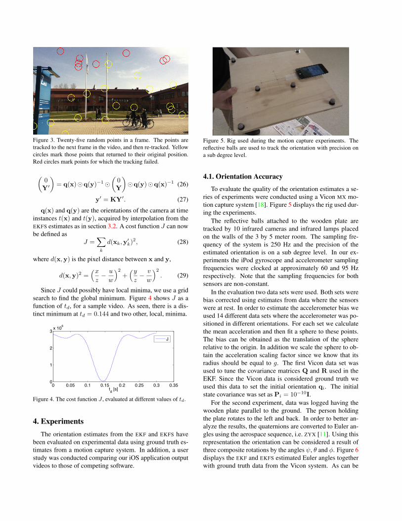
Figure 3. Twenty-five random points in a frame. The points are

tracked to the next frame in the video, and then re-tracked. Yellow

circles mark those points that returned to their original position.

Red circles mark points for which the tracking failed.

(

0Y′

)

= q(x)⊙q(y)−1 ⊙

(

0Y

)

⊙q(y)⊙q(x)−1 (26)

y′ = KY′. (27)

q(x) and q(y) are the orientations of the camera at time

instances t(x) and t(y), acquired by interpolation from the

EKFS estimates as in section 3.2. A cost function J can now

be defined as

J =∑

k

d(xk,y′k)2, (28)

where d(x,y) is the pixel distance between x and y,

d(x,y)2 =(x

z−u

w

)2

+(y

z−v

w

)2

. (29)

Since J could possibly have local minima, we use a grid

search to find the global minimum. Figure 4 shows J as a

function of td, for a sample video. As seen, there is a dis-

tinct minimum at td = 0.144 and two other, local, minima.

0 0.05 0.1 0.15 0.2 0.25 0.3 0.350

1

2

3x 10

6

td [s]

J

Figure 4. The cost function J , evaluated at different values of td.

4. Experiments

The orientation estimates from the EKF and EKFS have

been evaluated on experimental data using ground truth es-

timates from a motion capture system. In addition, a user

study was conducted comparing our iOS application output

videos to those of competing software.

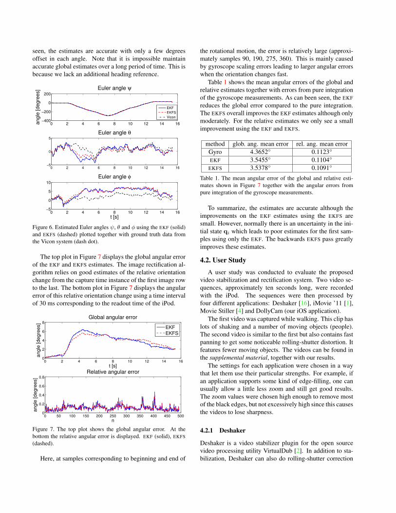
Figure 5. Rig used during the motion capture experiments. The

reflective balls are used to track the orientation with precision on

a sub degree level.

4.1. Orientation Accuracy

To evaluate the quality of the orientation estimates a se-

ries of experiments were conducted using a Vicon MX mo-

tion capture system [18]. Figure 5 displays the rig used dur-

ing the experiments.

The reflective balls attached to the wooden plate are

tracked by 10 infrared cameras and infrared lamps placed

on the walls of the 3 by 5 meter room. The sampling fre-

quency of the system is 250 Hz and the precision of the

estimated orientation is on a sub degree level. In our ex-

periments the iPod gyroscope and accelerometer sampling

frequencies were clocked at approximately 60 and 95 Hz

respectively. Note that the sampling frequencies for both

sensors are non-constant.

In the evaluation two data sets were used. Both sets were

bias corrected using estimates from data where the sensors

were at rest. In order to estimate the accelerometer bias we

used 14 different data sets where the accelerometer was po-

sitioned in different orientations. For each set we calculate

the mean acceleration and then fit a sphere to these points.

The bias can be obtained as the translation of the sphere

relative to the origin. In addition we scale the sphere to ob-

tain the acceleration scaling factor since we know that its

radius should be equal to g. The first Vicon data set was

used to tune the covariance matrices Q and R used in the

EKF. Since the Vicon data is considered ground truth we

used this data to set the initial orientation qi. The initial

state covariance was set as Pi = 10−10I.

For the second experiment, data was logged having the

wooden plate parallel to the ground. The person holding

the plate rotates to the left and back. In order to better an-

alyze the results, the quaternions are converted to Euler an-

gles using the aerospace sequence, i.e. ZYX [11]. Using this

representation the orientation can be considered a result of

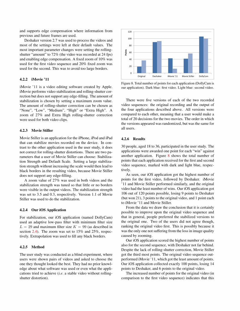
three composite rotations by the angles ψ, θ and φ. Figure 6

displays the EKF and EKFS estimated Euler angles together

with ground truth data from the Vicon system. As can be

seen, the estimates are accurate with only a few degrees

offset in each angle. Note that it is impossible maintain

accurate global estimates over a long period of time. This is

because we lack an additional heading reference.

0 2 4 6 8 10 12 14 16−400

−200

0

200

Euler angle ψ

an

gle

[d

eg

ree

s]

0 2 4 6 8 10 12 14 16−5

0

5

Euler angle θ

0 2 4 6 8 10 12 14 16−5

0

5

10

Euler angle φ

t [s]

EKF

EKFS

Vicon

Figure 6. Estimated Euler angles ψ, θ and φ using the EKF (solid)

and EKFS (dashed) plotted together with ground truth data from

the Vicon system (dash dot).

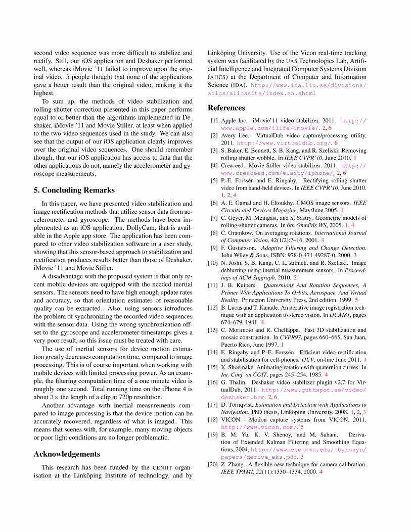
The top plot in Figure 7 displays the global angular error

of the EKF and EKFS estimates. The image rectification al-

gorithm relies on good estimates of the relative orientation

change from the capture time instance of the first image row

to the last. The bottom plot in Figure 7 displays the angular

error of this relative orientation change using a time interval

of 30 ms corresponding to the readout time of the iPod.

0 2 4 6 8 10 12 14 160

2

4

6

8

Global angular error

t [s]

an

gle

[d

eg

ree

s]

0 50 100 150 200 250 300 350 400 450 5000

0.2

0.4

0.6

0.8

Relative angular error

n

an

gle

[d

eg

ree

s]

EKF

EKFS

Figure 7. The top plot shows the global angular error. At the

bottom the relative angular error is displayed. EKF (solid), EKFS

(dashed).

Here, at samples corresponding to beginning and end of

the rotational motion, the error is relatively large (approxi-

mately samples 90, 190, 275, 360). This is mainly caused

by gyroscope scaling errors leading to larger angular errors

when the orientation changes fast.

Table 1 shows the mean angular errors of the global and

relative estimates together with errors from pure integration

of the gyroscope measurements. As can been seen, the EKF

reduces the global error compared to the pure integration.

The EKFS overall improves the EKF estimates although only

moderately. For the relative estimates we only see a small

improvement using the EKF and EKFS.

method glob. ang. mean error rel. ang. mean error

Gyro 4.3652◦ 0.1123◦

EKF 3.5455◦ 0.1104◦

EKFS 3.5378◦ 0.1091◦

Table 1. The mean angular error of the global and relative esti-

mates shown in Figure 7 together with the angular errors from

pure integration of the gyroscope measurements.

To summarize, the estimates are accurate although the

improvements on the EKF estimates using the EKFS are

small. However, normally there is an uncertainty in the ini-

tial state qi which leads to poor estimates for the first sam-

ples using only the EKF. The backwards EKFS pass greatly

improves these estimates.

4.2. User Study

A user study was conducted to evaluate the proposed

video stabilization and rectification system. Two video se-

quences, approximately ten seconds long, were recorded

with the iPod. The sequences were then processed by

four different applications: Deshaker [16], iMovie ’11 [1],

Movie Stiller [4] and DollyCam (our iOS application).

The first video was captured while walking. This clip has

lots of shaking and a number of moving objects (people).

The second video is similar to the first but also contains fast

panning to get some noticeable rolling-shutter distortion. It

features fewer moving objects. The videos can be found in

the supplemental material, together with our results.

The settings for each application were chosen in a way

that let them use their particular strengths. For example, if

an application supports some kind of edge-filling, one can

usually allow a little less zoom and still get good results.

The zoom values were chosen high enough to remove most

of the black edges, but not excessively high since this causes

the videos to lose sharpness.

4.2.1 Deshaker

Deshaker is a video stabilizer plugin for the open source

video processing utility VirtualDub [2]. In addition to sta-

bilization, Deshaker can also do rolling-shutter correction

and supports edge compensation where information from

previous and future frames are used.

Deshaker version 2.7 was used to process the videos and

most of the settings were left at their default values. The

most important parameter changes were setting the rolling-

shutter “amount” to 72% (the video was recorded at 24 fps)

and enabling edge compensation. A fixed zoom of 10% was

used for the first video sequence and 20% fixed zoom was

used for the second. This was to avoid too large borders.

4.2.2 iMovie ’11

iMovie ’11 is a video editing software created by Apple.

iMovie performs video stabilization and rolling-shutter cor-

rection but does not support any edge-filling. The amount of

stabilization is chosen by setting a maximum zoom value.

The amount of rolling-shutter correction can be chosen as

“None”, “Low”, “Medium”, “High” or “Extra High”. A

zoom of 27% and Extra High rolling-shutter correction

were used for both video clips.

4.2.3 Movie Stiller

Movie Stiller is an application for the iPhone, iPod and iPad

that can stabilize movies recorded on the device. In con-

trast to the other application used in the user study, it does

not correct for rolling-shutter distortions. There are two pa-

rameters that a user of Movie Stiller can choose: Stabiliza-

tion Strength and Default Scale. Setting a large stabiliza-

tion strength without increasing the scale would then lead to

black borders in the resulting video, because Movie Stiller

does not support any edge-filling.

A zoom value of 27% was used in both videos and the

stabilization strength was tuned so that little or no borders

were visible in the output videos. The stabilization strength

was set to 3.5 and 0.3, respectively. Version 1.1 of Movie

Stiller was used to do the stabilization.

4.2.4 Our iOS Application

For stabilization, our iOS application (named DollyCam)

used an adaptive low-pass filter with minimum filter size

L = 29 and maximum filter size K = 99 (as described in

section 2.4). The zoom was set to 15% and 25%, respec-

tively. Extrapolation was used to fill any black borders.

4.2.5 Method

The user study was conducted as a blind experiment, where

users were shown pairs of videos and asked to choose the

one they thought looked the best. They had no prior knowl-

edge about what software was used or even what the appli-

cations tried to achieve (i.e. a stable video without rolling-

shutter distortion).

80

100

120

ints

0

20

40

60

80

100

120

Original Deshaker iMovie '11 Movie Stiller DollyCam

Po

ints

Figure 8. Total number of points for each application (DollyCam is

our application). Dark blue: first video. Light blue: second video.

There were five versions of each of the two recorded

video sequences: the original recording and the output of

the four applications described above. All versions were

compared to each other, meaning that a user would make a

total of 20 decisions for the two movies. The order in which

the versions appeared was randomized, but was the same for

all users.

4.2.6 Results

30 people, aged 18 to 36, participated in the user study. The

applications were awarded one point for each “win” against

another application. Figure 8 shows the total number of

points that each application received for the first and second

video sequence, marked with dark and light blue, respec-

tively.

As seen, our iOS application got the highest number of

points for the first video, followed by Deshaker. iMovie

’11 and Movie Stiller performed similarly, and the original

video had the least number of wins. Our iOS application got

106 out of 120 points possible, losing 9 points to Deshaker

(but won 21), 3 points to the original video, and 1 point each

to iMovie ’11 and Movie Stiller.

From the data we draw the conclusion that it is certainly

possible to improve upon the original video sequence and

that in general, people preferred the stabilized versions to

the original one. Two of the users did not agree though,

ranking the original video first. This is possibly because it

was the only one not suffering from the loss in image quality

caused by zooming.

Our iOS application scored the highest number of points

also for the second sequence, with Deshaker not far behind.

Despite the lack of rolling-shutter correction, Movie Stiller

got the third most points. The original video sequence out-

performed iMovie ’11, which got the least amount of points.

Our iOS application collected exactly 100 points, losing 14

points to Deshaker, and 6 points to the original video.

The increased number of points for the original video (in

comparison to the first video sequence) indicates that this

second video sequence was more difficult to stabilize and

rectify. Still, our iOS application and Deshaker performed

well, whereas iMovie ’11 failed to improve upon the orig-

inal video. 5 people thought that none of the applications

gave a better result than the original video, ranking it the

highest.

To sum up, the methods of video stabilization and

rolling-shutter correction presented in this paper performs

equal to or better than the algorithms implemented in De-

shaker, iMovie ’11 and Movie Stiller, at least when applied

to the two video sequences used in the study. We can also

see that the output of our iOS application clearly improves

over the original video sequences. One should remember

though, that our iOS application has access to data that the

other applications do not, namely the accelerometer and gy-

roscope measurements.

5. Concluding Remarks

In this paper, we have presented video stabilization and

image rectification methods that utilize sensor data from ac-

celerometer and gyroscope. The methods have been im-

plemented as an iOS application, DollyCam, that is avail-

able in the Apple app store. The application has been com-

pared to other video stabilization software in a user study,

showing that this sensor-based approach to stabilization and

rectification produces results better than those of Deshaker,

iMovie ’11 and Movie Stiller.

A disadvantage with the proposed system is that only re-

cent mobile devices are equipped with the needed inertial

sensors. The sensors need to have high enough update rates

and accuracy, so that orientation estimates of reasonable

quality can be extracted. Also, using sensors introduces

the problem of synchronizing the recorded video sequences

with the sensor data. Using the wrong synchronization off-

set to the gyroscope and accelerometer timestamps gives a

very poor result, so this issue must be treated with care.

The use of inertial sensors for device motion estima-

tion greatly decreases computation time, compared to image

processing. This is of course important when working with

mobile devices with limited processing power. As an exam-

ple, the filtering computation time of a one minute video is

roughly one second. Total running time on the iPhone 4 is

about 3× the length of a clip at 720p resolution.

Another advantage with inertial measurements com-

pared to image processing is that the device motion can be

accurately recovered, regardless of what is imaged. This

means that scenes with, for example, many moving objects

or poor light conditions are no longer problematic.

Acknowledgements

This research has been funded by the CENIIT organ-

isation at the Linkoping Institute of technology, and by

Linkoping University. Use of the Vicon real-time tracking

system was facilitated by the UAS Technologies Lab, Artifi-

cial Intelligence and Integrated Computer Systems Division

(AIICS) at the Department of Computer and Information

Science (IDA). http://www.ida.liu.se/divisions/

aiics/aiicssite/index.en.shtml

References

[1] Apple Inc. iMovie’11 video stabilizer, 2011. http://

www.apple.com/ilife/imovie/. 2, 6

[2] Avery Lee. VirtualDub video capture/processing utility,

2011. http://www.virtualdub.org/. 6

[3] S. Baker, E. Bennett, S. B. Kang, and R. Szeliski. Removing

rolling shutter wobble. In IEEE CVPR’10, June 2010. 1

[4] Creaceed. Movie Stiller video stabilizer, 2011. http://

www.creaceed.com/elasty/iphone/. 2, 6

[5] P.-E. Forssen and E. Ringaby. Rectifying rolling shutter

video from hand-held devices. In IEEE CVPR’10, June 2010.

1, 2, 4

[6] A. E. Gamal and H. Eltoukhy. CMOS image sensors. IEEE

Circuits and Devices Magazine, May/June 2005. 1

[7] C. Geyer, M. Meingast, and S. Sastry. Geometric models of

rolling-shutter cameras. In 6th OmniVis WS, 2005. 1, 4

[8] C. Gramkow. On averaging rotations. International Journal

of Computer Vision, 42(1/2):7–16, 2001. 3

[9] F. Gustafsson. Adaptive Filtering and Change Detection.

John Wiley & Sons, ISBN: 978-0-471-49287-0, 2000. 3

[10] N. Joshi, S. B. Kang, C. L. Zitnick, and R. Szeliski. Image

deblurring using inertial measurement sensors. In Proceed-

ings of ACM Siggraph, 2010. 2

[11] J. B. Kuipers. Quaternions And Rotation Sequences, A

Primer With Applications To Orbits, Aerospace, And Virtual

Reality. Princeton University Press, 2nd edition, 1999. 5

[12] B. Lucas and T. Kanade. An iterative image registration tech-

nique with an application to stereo vision. In IJCAI81, pages

674–679, 1981. 4

[13] C. Morimoto and R. Chellappa. Fast 3D stabilization and

mosaic construction. In CVPR97, pages 660–665, San Juan,

Puerto Rico, June 1997. 1

[14] E. Ringaby and P.-E. Forssen. Efficient video rectification

and stabilisation for cell-phones. IJCV, on-line June 2011. 1

[15] K. Shoemake. Animating rotation with quaternion curves. In

Int. Conf. on CGIT, pages 245–254, 1985. 4

[16] G. Thalin. Deshaker video stabilizer plugin v2.7 for Vir-

tualDub, 2011. http://www.guthspot.se/video/

deshaker.htm. 2, 6

[17] D. Tornqvist. Estimation and Detection with Applications to

Navigation. PhD thesis, Linkoping University, 2008. 1, 2, 3

[18] VICON - Motion capture systems from VICON, 2011.

http://www.vicon.com/. 5

[19] B. M. Yu, K. V. Shenoy, and M. Sahani. Deriva-

tion of Extended Kalman Filtering and Smoothing Equa-

tions, 2004. http://www.ece.cmu.edu/˜byronyu/

papers/derive_eks.pdf. 3

[20] Z. Zhang. A flexible new technique for camera calibration.

IEEE TPAMI, 22(11):1330–1334, 2000. 4