special issue: the econometrics of financial markets || an empirical assessment of non-linearities...

The Review of Economic Studies, Ltd.

An Empirical Assessment of Non-Linearities in Models of Exchange Rate DeterminationAuthor(s): Richard A. Meese and Andrew K. RoseReviewed work(s):Source: The Review of Economic Studies, Vol. 58, No. 3, Special Issue: The Econometrics ofFinancial Markets (May, 1991), pp. 603-619Published by: Oxford University PressStable URL: http://www.jstor.org/stable/2298014 .

Accessed: 22/02/2013 13:17

Your use of the JSTOR archive indicates your acceptance of the Terms & Conditions of Use, available at .http://www.jstor.org/page/info/about/policies/terms.jsp

.JSTOR is a not-for-profit service that helps scholars, researchers, and students discover, use, and build upon a wide range ofcontent in a trusted digital archive. We use information technology and tools to increase productivity and facilitate new formsof scholarship. For more information about JSTOR, please contact [email protected].

.

Oxford University Press and The Review of Economic Studies, Ltd. are collaborating with JSTOR to digitize,preserve and extend access to The Review of Economic Studies.

http://www.jstor.org

This content downloaded on Fri, 22 Feb 2013 13:17:15 PMAll use subject to JSTOR Terms and Conditions

http://www.jstor.org/action/showPublisher?publisherCode=oup

http://www.jstor.org/stable/2298014?origin=JSTOR-pdf

http://www.jstor.org/page/info/about/policies/terms.jsp


Review of Economic Studies (1991) 58, 603-619 0034-6527/91/00360603$02.00

? 1991 The Review of Economic Studies Limited

An Empirical Assessment of

Non-Linearities in Models of

Exchange Rate Determination RICHARD A. MEESE

and ANDREW K. ROSE

University of California, Berkeley

First version received September 1989; final version accepted September 1990 (Eds.)

This paper examines the empirical relation between nominal exchange rates and macroeconomic fundamentals for five major OECD countries between 1974 and 1987. Five theoretical models of exchange rate determination are considered. Potential non-linearities are examined using a variety of parametric and non-parametric techniques. We find that the poor explanatory power of the models considered cannot be attributed to non-linearities arising from time-deformation or improper functional form.

I. INTRODUCTION

It is now recognized that empirical exchange rate models of the post-Bretton Woods era are characterized by parameter instability and dismal forecast performance. For instance, Meese and Rogoff (1983) have shown that a simple random walk forecasts as well as most linear exchange rate models. In this paper, we assess the importance of non- linearities in empirical models of the exchange rate. In particular, we test the hypothesis that non-linear extensions of existing structural models of exchange rates perform significantly better than existing (linear) models.

Recent research has convincingly demonstrated the importance of non-linearities in exchange rates. The univariate distribution of (high frequency) exchange rate changes is known to be leptokurtic (Westerfield (1977), Boothe and Glassman (1987) and Hsieh (1988)). Researchers have also found conditional heteroskedasticity in the residuals of both time-series and structural models of spot exchange rates (e.g. Cumby and Obstfeld (1984), Domowitz and Hakkio (1985), Hsieh (1989) and Engle, Ito and Lin (1990)). However, the existence of residual conditional heteroskedasticity or leptokurtosis in exchange returns, may not improve our ability to explain the levels of exchange rates, since these effects operate through even-ordered moments. This point is made forcefully in a recent paper by Diebold and Nason (1990). They employ univariate non-parametric time-series methods to forecast the conditional mean of spot exchange rates, but find little improvement in predictive accuracy over a simple random walk.

One of the very few papers that attempts to test structural multivariate models of the exchange rate with non-linear techniques is Schinasi and Swamy (1989).' They show that non-linear random coefficients techniques sometimes lead to improved forecasting

1. Of related interest are the papers by Chinn (1991), Diebold and Pauly (1988) and Engel and Hamilton (1990).

603



604 REVIEW OF ECONOMIC STUDIES

ability of exchange rate models. The analysis by Schinasi and Swamy is conducted over one short forecast period; average parameter values are unfortunately not reported. Nevertheless, such findings suggest that taking proper account of non-linearities may improve our understanding of the determinants of exchange rates.

The techniques that we use in this paper are intended to isolate non-linearities that are both economically meaningful and affect the level of the exchange rate. That is, we are interested in testing for a nonlinear relationship between the exchange rate and fundamentals, rather than nonlinear serial dependence in moments of the univariate exchange rate distribution.

In this paper, we consider five structural exchange rate models, and account for potential non-linearities in these models in three ways. First, we examine the possibility that economic events take place on a time scale that differs from calendar time, recently dubbed "time-deformation" by Stock (1987). Next, we employ a non-parametric procedure to estimate the functional form of our exchange rate models, thus accounting for potential mis-specifications of utility, production and demand for money functions in standard linear models. Finally, we consider whether non-linear exchange rate dynamics might arise for intrinsic economic reasons. Much recent research has focussed on the possibility that non-linear dynamics arise from the nature of the policy regime (Flood and Garber (1983), Krugman (1988), and Froot and Obstfeld (1989); see also Kaminsky (1989)). The statistical procedures which we use can easily handle the non-linearities relevant to this literature, but are much more general, and can be used to estimate structural models without many of the restrictions typically employed in empirical work.

Despite the generality and multiplicity of our techniques, our empirical results are negative. We do not deny that non-linear effects are important in understanding even moments of exchange rate processes. However, we do conclude that incorporating non-linearities into existing structural models of exchange rate determination does not at present appear to be a research strategy which is likely to improve dramatically our ability to understand how exchange rates are determined.

The paper is organized as follows. Section II contains a brief review of the theoretical exchange rate models which we consider; Section III provides a variety of rationalizations for non-linearities in these models. Section IV contains a description of the data, and some preliminary diagnostics. Our three non-linear techniques are presented in the next three sections. Section V contains tests for time-deformation; Section VI presents non- parametric functional form estimates; Section VII is concerned with non-parametric regression analysis. Finally, Section VIII is a brief conclusion.

II. FIVE STRUCTURAL EXCHANGE RATE MODELS

The first three models of exchange rate determination which we consider are variants of the popular monetary models of Dornbusch (1976), Frenkel (1976), and Mussa (1976). All three models consist of a conventional well-specified domestic money demand equation with stationary disturbance,2 an analogous foreign money demand equation, and an equation relating the expected change in the spot rate to the interest differential, and an exogenously-varying risk premium on domestic assets (which may equal zero). More thorough reviews of exchange rate theories, are available in The Handbook of International Economics.

2. Mis-specified money demand functions will result in mis-specified exchange rate equations. Ericsson and Hendry (1990) provide evidence on the stability of money demand functions in two countries.



MEESE & ROSE EXCHANGE RATE DETERMINATION 605

The flexible-price monetary model (our first model) assumes purchasing power parity (PPP) holds up to an exogenous real exchange rate shock. The sticky-price variants (our second and third models) assume slow adjustment of goods prices relative to asset prices, and thus allow deviations from PPP to be slowly damped. One version of our sticky-price monetary model does not contain cumulated domestic and foreign trade balances, while the other does. The trade balance term can arise, for example, when wealth is included in the money demand equations. All three models are subsumed in:

s =f(m, ip, r, p, tb) + error (1)

where: s is the bilateral spot exchange rate (measured as the domestic price of a unit of foreign exchange, e.g. $/DM); m denotes the relative (ratio of domestic to foreign) nominal money supply; ip denotes relative industrial production; r denotes the nominal interest differential; p denotes the inflation differential; and tb denotes the relative cumulated trade balances. The properties of the error term are considered explicitly below, for both parametric and non-parametric specifications of (1).

The flexible-price monetary model imposes the restriction that p and tb do not enter equation (1). The first sticky-price monetary model imposes the constraint that trade balances do not enter (1), and in addition, assumes that the real interest differential, r -p is an appropriate explanatory variable. The second sticky-price monetary model also employs the real interest differential, but has no restriction on the trade balance term.

The second group of exchange rate models which we consider is based on explicit maximizing behaviour. The first is a variant of the highly-stylized Lucas (1982) model of a two-good, two-country, pure-exchange economy. A representative agent who con- sumes both foreign and domestic output maximizes the expected discounted utility of current and future consumption subject to budget and cash in advance constraints. The solution for the spot exchange rate is the product of relative monies, incomes and the marginal rate of substitut-ion between domestic and foreign goods. We parametrize the model by assuming a Cobb-Douglas utility function. This in turn implies that the spot exchange rate can be simply related to relative money supplies and domestic outputs;3

s=f(m, ip)+error. (2)

Our fifth and final model is Hodrick's (1988) extension of Svensson's exchange rate model (1985a, b). The basic framework is that of Lucas (1982) with a modification of the timing of goods and money market transactions. Hodrick's contribution is to add exogenous fiscal policy and examine the effect of time-varying conditional variances of the exogenous processes on the level of the spot rate. A version of Hodrick's model can be parameterized as:

s=f(m, ip, 8m, h(m), h(ip), h(8m))+error, (3)

where 8m is the change in relative money growth rates, and h( -) denotes the conditional variance of the variable in parentheses.4

III. POTENTIAL SOURCES OF NON-LINEARITIES

There are two separate motivations for our concern with non-linear exchange rate models. Observable data may be related in some non-linear fashion to an intrinsically linear but unobservable data generation process (DGP); alternatively, the data generation process may be intrinsically non-linear. In this section, we briefly discuss these issues in turn.

3. The Lucas model is observationally equivalent to the particular solution to a flexible-price exchange rate model with random-walk fundamentals; Krugman (1990).

4. The lack of parsimony in the Hodrick model renders some statistical procedures below intractable.




One potential source of non-linearities in exchange rate models is the possibility that economic time and calendar time might differ. For example, the appropriate time scale for currency markets might "speed up" in calendar time in periods when an usually large amount of news must be processed by the market. Clark's (1973) model of this phenomenon subordinates asset prices to an information arrival process; Clark shows how this framework can potentially explain the observed leptokurtosis in asset returns. Stock (1987) explores the possibility that the relationship between economic and calendar time depends on the economic history of certain variables which indicate acceleration or deceleration of economic time. He develops a test statistic for time-deformation which amounts to a set of linear restrictions in a vector autoregression (VAR). Time-deformation test results are reported in the next section.

Time-deformation is not the only reason why an intrinsically linear data-generation process may be poorly modelled by linear empirical models. Mis-specification of the functional form in the empirical model may also lead to manifestations of non-linearities. The widely used logarithmic transformation has a number of attractive features (e.g. it allows coefficients to be interpreted as elasticities, and ensures positivity of the fitted dependent variable). However, economic theory rarely implies that the log transformation is appropriate. While the log transformation is testable, in practice it is rarely tested. As inappropriate functional form (e.g. application of the log transformation) can lead to apparently non-linear manifestations of model mis-specification, it seems worthwhile to test the functional form of structural exchange ratea models. Recent advances in non- parametric and semi-parametric regression techniques allow statistical inference to be conducted with few assumptions regarding functional form.

Alternatively, the data-generation process itself may be intrinsically non-linear. A curent class of rational expectations models is intrinsically non-linear. In these models, forward-looking agents forecast the future time-path of fundamentals; however, if agents expect that government reaction functions are subject to stochastic change, or that the authorities will regulate the fundamentals driving the exchange rate when the latter approaches or reaches the band of a "target zone", then the appropriate prediction formula (and hence, reduced-form exchange rate equation) may have a complicated non-linear form. Recent research on the possibility of stochastic regime changes and target zones in exchange rate models includes: Engel and Hamilton (1990); Flood and Garber (1983); Flood and Rose (1990); Froot and Obstfeld (1989); Krugman (1990); and Meese and Rose (1990). Closed-form solutions have been found for models without inertia, such as our first model, the flexible-price monetary model. When agents assign a non-zero probability to a regime change (such as a policy of increased currency market intervention when the exchange rate approaches some pre-announced barrier), Krugman shows that the exchange rate solution contains both the conventional linear terms of equation (1), and a set of non-linear terms in current fundamentals. A formal test for this type of non-linear mis-specification in our five representative exchange rate equations is presented below.

IV. DATA AND PRELIMINARY DIAGNOSTICS

Data

All of the data are taken from the OECD's Main Economic Indicators, including measures of:bilateral exchange rates (vis-a-vis the U.S. dollar); exports; imports; industrial production indices (used as the proxy for real output); the CPI (used as the price proxy); the money supply (Ml); and the short-term interest rate. All data has been transformed into




differentials between foreign and U.S. values. The data are monthly, seasonally adjusted, and span 1974 through 1987. The trade flow data is deflated by the CPI. Unless noted, natural logarithms are taken of all variables except for the trade balance and the short-term interest rate; we investigate the validity of such transformations below.

Unit-roots

We test for manifestations of non-stationarity, both as a first step in exploring the characteristics of the data, and since the presence of such nonstationarity often has important econometric implications (Stock and Watson (1988) provide a recent survey).

A variable x is said to have a unit-root in its autoregressive process if its autoregressive representation is of the form:

(1 -L)xt = (lJ1- L)xtI 1+ * * *+p(l -L)xt-p +Et

where s is a stationary stochastic process, E (Di < 1, and Lkx Xt-k.

A number of statistics have been proposed as tests for the existence of unit-roots. We use the well-known Dickey-Fuller test (augmented in this case by four lags of the differenced variables, as well as a constant), which can be computed by running the regression:

(1- L)xt = a +8xtI +Yj=i bi(l - L)xt-i + Et

A large negative estimate of /8 is inconsistent with the null hypothesis of a unit-root in x. Table I reports Dickey-Fuller tests for unit-roots for the variables in our first four

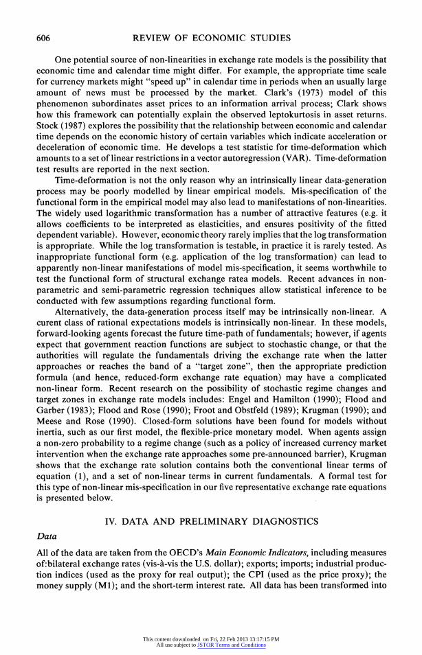
models (relaxing the differential form of the explanatory variables does not change results). The sample period is 1974:1 through 1987:12, so that 168 observations are included; critical values are also reported. Also reported are the non-parametric unit-root tests suggested by Perron (1988), which impose less structure on the process of the disturbance term {?}. A constant term is incorporated in the Perron tests so that the same critical values apply to both sets of unit-root tests.5

TABLE I

Unit-root tests

Canada Germany Japan U. K.

Augmented Dickey-Fuller Tests Exchange Rate -1 15 0 77 1 08 0-31 Nominal Interest Rate -3 86 -4 52 -2 41 -3 20 Real Interest Rate -2-94 -2-86 -3-27 -2-73 Money -0 16 -0 55 -0-23 -0-02 Domestic Output -2 79 -1 09 -1 64 -1 43 Cumulated Trade Balance 1-49 2-09 0-71 1-23

Perron Tests Exchange Rate -1-56 -1-36 -0-18 -1 98 Nominal Interest Rate -4-02 -4-21 -2-49 -2-60 Real Interest Rate -3.40 -3 02 -3 00 -1-34 Money -0-54 -0 60 -0 11 -0-43 Domestic Output -2-63 -1-86 -1-49 -1P87 Cumulated Trade Balance 10-34 11-43 10-16 8-82

Note. Critical Values for rejecting null hypothesis of unit-root: (0-01)-3.50; (0-05)-2 89; (0 1)- 2 58.

5. Twelve lags are used to construct the estimated variance of the disturbance process, so that the Perron tests are estimated with 156 observations. Including a deterministic trend (and using appropriate critical values) does not change any conclusions. Results are also insensitive to exact choice of sample period, as well as the exact number of augmenting lags.




The test statistics are consistent with the hypothesis that unit-root non-stationarity characterizes most of the variables. The null hypothesis of a unit-root in the univariate representation cannot be rejected for any of the variables at reasonable significance levels, except for some of the interest rate differentials.6 As a result, we choose to use first- differences in much of our analysis below, noting that the first-difference of a stationary series is also stationary. We also note that the use of potentially stationary interest differentials affects tests for co-integration, a topic we now pursue.

Co-integration

If unit-root non-stationarity characterizes the DGP of the variables of interest, "co- integration" is a pre-condition for the existence of a stable, linear relationship between the exchange rate and the relevant explanatory variables given by each of our structural models. A vector of variables is co-integrated if each variable in the vector individually contains a unit-root, but a linear combination of the variables is stationary.

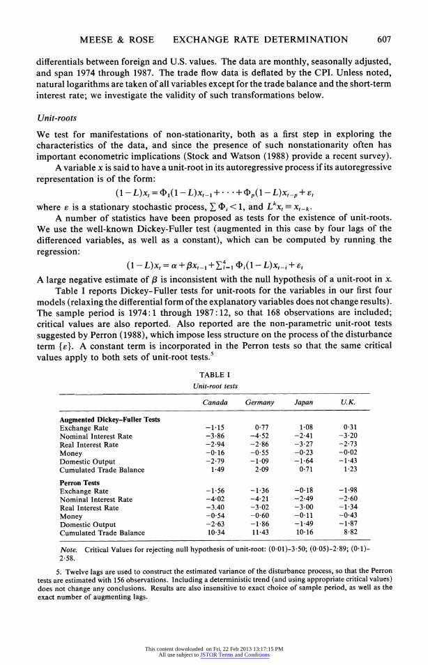
Table II contains the augmented Dickey-Fuller ("ADF") tests recommended by Engle and Granger (1987). These tests are tests for a unit-root of the residual from a "co-integrating" regression of the (logarithm of the) bilateral exchange rate on the relevant explanatory variables.7 Rejection of the null hypothesis is a rejection of the hypothesis of no co-integration. As in Table I, the sample period is 74:1 through 87:12, and the Dickey-Fuller tests are augmented by four lagged differences of the residual. Critical values drawn from Engle and Yoo (1987) are also included.

The presence of potentially stationary interest differentials may invalidate some of the Engle-Granger tests. Therefore, Table II also includes the results of tests for the number of co-integrating vectors proposed by Johansen (1988). This procedure allows for potentially stationary variables, and has the further benefit of greater power than the

TABLE II

Co-integration tests

Engle and Granger Augmented Dickey-Fuller Tests

Model Canada Germany Japan U.K.

Lucas -3-20 -0-72 -0 75 -1 12 Flexible-price -3*08 -0*76 -1*96 -1*02 Sticky-price 1 -3-08 -1-69 -2-03 -1-34 Sticky-price 2 -1-31 -3 79 -3-62 -1-36 0-10 Critical values for rejection of null hypothesis of no co-integration: Lucas Model -3 5; Flexible-price and Sticky-price 1 -3-8; Sticky-price 2 -4-2.

Johansen Tests (Number of co-integrating vectors without/with exchange rate)


Lucas 0/2 1/0 1/1 0/0 Flexible-price 1/1 2/1 2/2 1/0 Sticky-price 1 1/1 1/0 1/1 1/1 Sticky-price 2 3/2 3/3 4/3 3/2

6. In monetary exchange rate models, the nominal interest differential is the proxy for expected depreciation, less a possible risk premium on domestic assets. Under rational expectations, expected depreciation is actual depreciation less a forecast error. The finding of stationary interest differentials is consistent with stationary forecast errors for expected depreciation and a stationary risk premium.

7. Again, relaxing the differential form of the explanatory variables does not change results.




Engle and Granger test, as it incorporates system dynamics. The number of co-integrating vectors indicated at the 0-05 level by the Johansen procedure is tabulated in Table II. Two statistics are reported for each model: the number of co-integrating vectors warranted in a system composed of the explanatory variables (e.g. differentials of logs of money, output and nominal interest rates in the flexible-price model); and the number of co-integrating vectors when the (log of the) exchange rate is added to the system. If the exchange rate is co-integrated with the explanatory variables, its addition to the system consisting of the latter should increase the number of co-integrating vectors by one.8

The results do not indicate linear co-integration for any exchange rate. None of the Engle and Granger tests is significant even at the 0.10 significance level. The Johansen tests indicate that when the exchange rate is added to a system consisting of the explanatory variables implied by a given structural model, another co-integrating vector is not generally found; that is, the number of co-integrating vectors does not generally rise with the addition of the exchange rate. Succinctly, the results in table II indicate that the linear relationship between exchange rates and the fundamentals of the four structural models is tenuous at best. As a result, in much of the analysis below, all of the variables will be first-differenced.

V. TIME-DEFORMATION

Stock (1987) suggests a simple test for time-deformation. The test requires estimation of the following unrestricted system of equations for Y(t), the first difference of the time t observations of all the variables (dependent and explanatory) in the model:

Y= C?+ C(L) t_J+C2 (L)zt,_+ C3(L)zt,_ Yt,1+et where C1(L) and C3(L) denote matrix polynomials of order P in the lag operator; C2(L) is scalar, of order P; zt denotes a scalar indicator variable for the change of time scale; and et is a normally distributed iid error term. The hypothesis of no time-deformation is a joint test of the linear constraints C2(L)= C3(L)=0. It should be noted that the validity of this test rests upon the assumption that the exchange rate model is correctly specified; that is, the test is observationally equivalent to a standard mis-specification test for omitted variables.

Selective results are reported in Table III. We have experimented with a wide variety of indicator variables (zt); the results in Table III use as indicator variables the growth rates of: the nominal exchange rate (s); the inflation rate differential (p); the nominal interest rate differential (r); the money supply differential (m); and the industrial production differential (ip). Thus, for each model and each exchange rate, five F-tests are reported. A large statistic signifies a significant departure from the null hypothesis of no time deformation. Rejection of the null hypothesis at the 0 05 (0-01) level is marked by one (two) asterisk(s); critical values are also tabulated.

We have also examined a range of other indicator variables, including the growth rates of: the unemployment rate differential; the CPI differential; the real interest rate differential; and the real exchange rate differential; the levels of: the CPI differential; the real exchange rate; the nominal exchange rate; a residual from a co-integrating regression; a residual from a VAR in levels; conditional volatilities of variables; and the volume of gross bilateral financial transactions. None of these variables strongly indicates the presence of time-deformation. These results are also insensitive to the exact number of lags in the VARs, and to the exact sample period.

8. The VARs used to generate the Johansen tests are estimated with a constant and two lags over the sample 1974:3 through 1987:12.




TABLE III

F-tests of time-deformation

Indicator Canada Germany Japan U.K.

Lucas Model (Critical Value for Rejection of null hypothesis of no time-deformation: F(8, 153)=2-00 (2-65) at 0 05 (0 01))

s 1-89 2-41* 1 11 1-57 p 1-23 1-40 0-61 1-07 r 110 0 70 0 74 1-26 m 1-79 0-98 0-46 1-26 ip 1*96 0-46 1-96 1-13

Flexible-price Monetary Model (Critical value for Rejection of null hypothesis of no time-deformation: F(10, 149)=1 90 (2-45) at 0 05 (0 01))

s 1-52 2.16* 0-90 2.57** p 1-06 1.11 0-80 0-95 r 0-71 0 94 0 77 0-66 m 1-56 0-82 0 58 0-96 ip 1-33 1-04 2-41* 1-24

Sticky-price Monetary Model 1 (Critical Value for Rejection of Null hypothesis of no time-deformation: F(10, 149)=1 90 (2 45) at 0-05 at 0 05 (0.01))

s 1-48 1.91* 091 1-62 p 0-71 0-96 0-59 0-87 r 0-53 0 74 0-63 0 70 m 1 54 0 93 0-41 0-78 ip 1-38 1-31 1-83 1-37

Sticky-price Monetary Model 2 (Critical Value for Rejection of null hypothesis of no time-deformation: F(10, 145)=1-80 (2 30) at 0 05 (0 01))

s 1-32 1-98* 0.99 1-39 p 0-66 0-82 0-98 0-67 r 1-03 1 01 0-67 0-61 m 1-50 1-24 0-88 0-86 ip 1-15 1-36 1-63 1-18

Hodrick Model (Critical Value for Rejection of null hypothesis of no time-deformation: F(22, 125)=1-63 (2 00) at 0 05 (0 01))

s 094 077 1-28 094 p 2.08** 1-18 0-89 1-16 r 0-53 0-64 0-64 1-02 m 1.19 1-02 109 105 ip 0-77 1-44 1-39 093

For the indicator variables we have selected, there is no evidence that non-linearities in current exchange rate models can be attributed to time-deformation. Rejections of the null hypothesis of no time-deformation occur in a relatively random way across model, country and indicator variable. While some rejections emerge (for instance, the s indicator variable tends to indicate time-deformation at the 0-05 level for most models with the German data9), these are neither strong nor uniform. We conclude that there is little evidence of important time-deformation in exchange rates.10

9. The results of Diebold and Pauly (1988) indicate that this may be merely a manifestation of an exchange rate risk premium. The existence of such a premium would imply that our structural models are mis-specified; if this premium is correlated with the square of the exchange rate, our time-deformation test would typically reject the joint null hypothesis of no time deformation and correct specification, when the exchange rate is used as the indicator.

10. Researchers who cannot reject the presence of statistically significant autoregressive conditional heteroskedasticity in exchange rate models often appeal informally to the concept of time-deformation as an economic rationalization for their results. Our negative results on time-deformation imply that this informal appeal may not be tenable, at least at the frequencies examined.




VI. NON-PARAMETRIC FUNCTIONAL FORM ESTIMATION

In this section of the paper, we briefly describe and then implement a non-parametric technique to estimate optimally the functional form of the explanatory variables in a multiple linear regression model which links the exchange rate to its fundamental determinants. In particular, we look for potentially non-linear transformations of our fundamentals which might strengthen the apparently weak linear relationship between the fundamentals and the exchange rate.

Researchers seeking to understand a linear relationship between a set of explanatory variables (xi) and a dependent variable (yi) with regression techniques, often replace xi and yi with transformations of the raw variables, denoted F(xi) and fQ(yi). For example, economists often apply the logarithmic transformation (i.e. ( * )=Q( * )=logarithm (*)). Sometimes applied researchers test or estimate the nature of the transformation, though usually after restricting themselves to a particular parametric family of functions.

Breiman and Friedman (1985) suggest a non-parametric way of estimating data transformations (F(D*) and Q( *)) so as to minimize the expected mean squared error of the regression f1(yi)=I3'F(xi)+Ei. The essence of the methodology is a simple algorithm which estimates a series of alternating conditional expectations (hence the technique is known as the "ACE" algorithm). I(K*) is estimated conditionally for a given choice of fQ(); then fQ() is estimated conditioning on the estimate of ?( ). ACE operates iteratively; the transformations of all of the variables except one are treated as fixed, and the optimal transformation for the variable in question is estimated with a non-parametric "data smooth" technique. The algorithm then proceeds to the next variable; iterations continue until the equation mean squared-error has been minimized. This technique unravels the transformations that make the relationship between fQ(y) and ?(x) as linear as possible (using the mean squared-residual-error as a measure of departure from linearity).

Breiman and Friedman demonstrate theoretically that the ACE algorithm produces transformations which asymptotically converge to the optimal transformations."' ACE relies on only extremely weak distributional assumptions, and can handle a wide variety of non-linear transformations of the data. It should be noted that ACE does not treat the explanatory variables as fixed, instead treating the variables as if drawn from a joint distribution.

In finite samples, the results depend on a "data smooth" technique used to generate empirical estimates of the conditional expectations. Data smooth techniques estimate "regression surfaces" (in this case f( y) and ?(x)) in a non- or a semi-parametric fashion. For instance, the histogram is a data smooth; it divides the data into disjoint intervals and "smooths the data" by summing the number of data points in each interval. Many such techniques exist, (e.g. kernel and nearest neighbour techniques); Breiman and Friedman recommend the "super-smoother", which uses local linear fits with a varying window width, the latter determined by local cross-validation.

Results

In practice, ACE is often used to produce scatter plots of the transformed and untransfor- med variables. Monte Carlo experimentation indicates that such plots are often highly suggestive of transformations and functional forms present in the data-generation process.

11. I.e. the transformation which delivers the "maximal correlation" between ?(x) and Q(y), an unam- biguously defined concept.




We follow the graphical approach in this paper, and also pursue more formal statistical analysis. ACE normalizes the regression coefficients of the transformed regressions to unity, so that a scatter plot of the raw variable against the transformation reveals not only the shape of the relevant function, but also the sign of the coefficient. That is, a negative coefficient on an explanatory variable will show up as a negatively-sloped transformation. 12

We use ACE to estimate optimal transformations for our five structural models. Each equation is a regression of the bilateral exchange rate on the fundamentals dictated by the five structural models.

Recall that the hypothesis of no co-integration could not be rejected for the raw variables. Having estimated the optimal transformations with ACE, we first ask: is there evidence that the ACE-transformed variables are co-integrated? A positive answer might imply that linear models which use raw variables are mis-specified, insofar as only the absence of appropriate (non-linear) transformations of the variables would be responsible for the finding of no co-integrations between the raw variables. A finding of co-integration between the ACE-transformed variables can alternatively be characterized as a finding of non-linear co-integration (Hallman (1987)).

Co-integration tests for the ACE-transformed variables are in Table IV. The test statistics are comparable to those of Table II; they are augmented Dickey-Fuller tests for a unit-root in the residual from a linear co-integrating regression of the level of the (ACE-transformed) exchange rate on the levels of the relevant (ACE-transformed) determinants. To gauge the statistical significance of the test statistics, we generate critical values with the Monte Carlo method used by Engle and Yoo (1987)2l

TABLE IV

Augmented Dickey-Fuller co-integration tests with ACE-transformed variables


Flexible-price -2*69 -2 45 -3*60 -4*12 Sticky-price 1 -3-31 -4 09 -295 -4-47 Sticky-price 2 -6-72 -6-46 -5-91 -6-23 Lucas -3-51 -1-85 -2-64 -4-17

Note. Simulated Critical Values (010) for rejection of null hypothesis of no co-integration: Lucas Model -5-11; Flexible-price and Sticky-price 1 Models -6 05; Sticky-price Model 2 -6-91.

The test statistics of Table IV are consistent with the hypothesis that the exchange rate is not co-integrated with (potentially non-linear) transformations of the fundamental determinants posited by the four structural models. This conclusion is the same as that of Table II; there is no evidence of any stationary empirical counterpart to the posited structural models either linear or non-linear.'4

12. For ease of interpretation, the dependent variable transformation (Q()) is constrained to be linear. 13. In particular, we generate vectors of 198 observations of (the relevant number of) independent random

walks without drift and standard unit-normal innovations. After discarding the initial 30 observations, we estimate ACE transformations, estimate a co-integrating regression using the transformed variables, and compute the ADF test for a unit-root in the co-integrating residual. This procedure is then replicated 2000 times.

14. It would be interesting to add a formal Hausman-style test of non-linear functional form by comparing the linear fit of our models with the fit after transformation by ACE. Technical problems arise because rates of convergence of non-parametric estimators differ from those of standard parametric ones.




0.75-

0.50-

0.25

0.00- S.

-0.25 I I 0 - 0.050 0.025 0.000 0.025 0.050

FIGURE 1

Canadian money

0.3-

0.2 :

0.1

-0.0 J

-0.1 .

-0.2-

- 0.3 4 - 0.025 0.000 0.025 0.050

FIGURE 2

Canadian output

0.4-

0.3-

0.2-

0.1 -

-0.0-

- 0.1 '

-0.3- 4

- 0.21 'E

- 5.0 2.5 0.0 2.5 5.0

FIGURE 3

Canadian interest rate




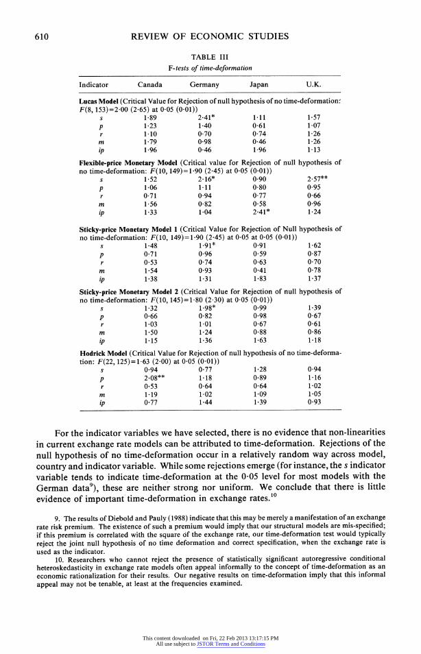
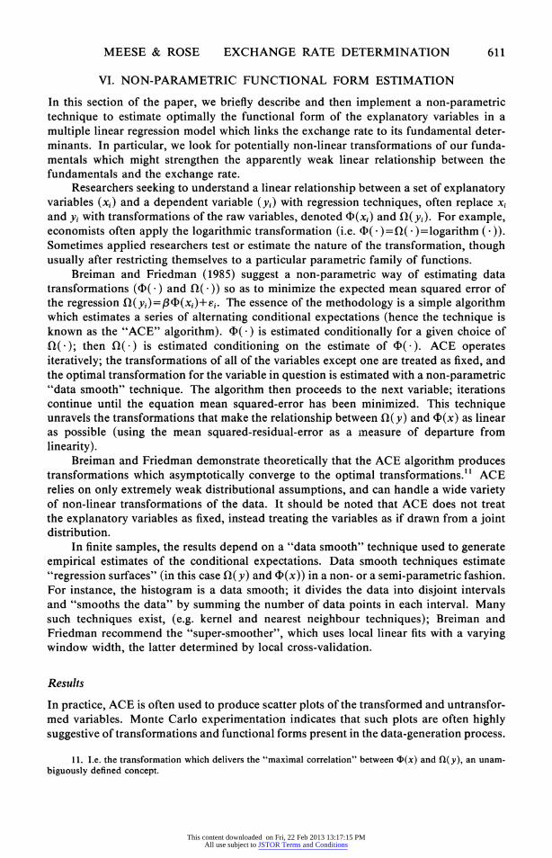
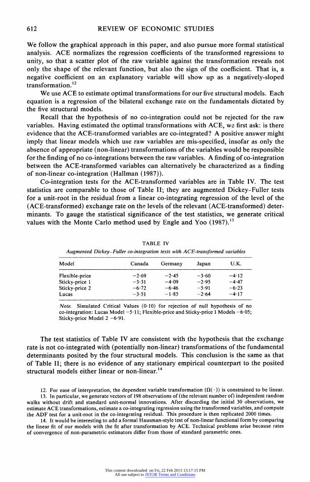
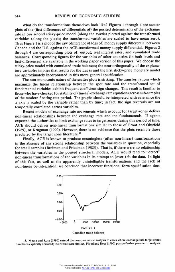
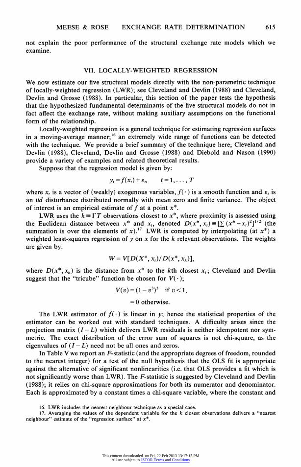
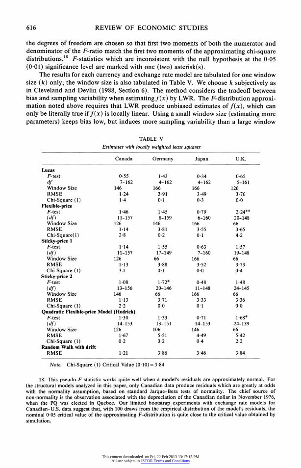
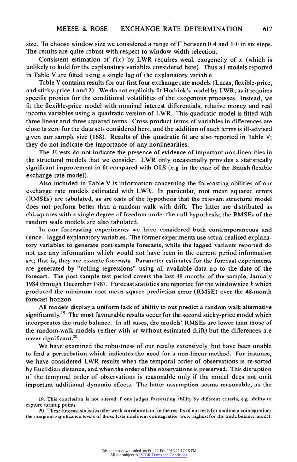
What do the transformations themselves look like? Figures 1 through 4 are scatter plots of the (first-differences of differentials of) the posited determinants of the exchange rate in our second sticky-price model (along the x-axis) plotted against the transformed variables (along the y-axis; the transformed variables are scaled to have mean zero). Thus Figure 1 is a plot of the raw (difference of logs of) money supply differential between Canada and the U.S. against the ACE-transformed money supply differential. Figures 2 through 4 are corresponding plots of: output; real interest rates; and cumulated trade balances. Corresponding figures for the variables of other countries (in both levels and first-differences) are available in the working paper version of this paper. We choose the sticky-price model with cumulated trade balances; the near orthogonality of the explanatory variables implies that results for the Lucas and the first sticky-price monetary model are approximately incorporated in this more general specification.

The non-monotonic nature of the scatter plots is striking. The transformations which maximize the linear relationship between the spot rate and the transformed set of fundamental variables exhibit frequent coefficient sign changes. This result is familiar to those who have checked for stability of (linear) exchange rate equations across sub-samples of the modern floating-rate period. The graphs should be interpreted with care since the x-axis is scaled by the variable rather than by time; in fact, the sign reversals are not temporally correlated across variables.

Recent models of exchange rate movements which account for target-zones deliver non-linear relationships between the exchange rate and the fundamentals. If agents expected the authorities to limit exchange rates to target zones during this period of time, ACE should deliver non-linear transformations similar to those of Froot and Obstfeld (1989), or Krugman (1990). However, there is no evidence that the plots resemble those predicted by the target zone literature.15

Finally, ACE is known to produce meaningless (often non-linear) transformations in the absence of any strong relationship between the variables in question, especially for small samples (Breiman and Friedman (1985)). That is, if there were no relationship between the variables in the posited structural models, ACE would tend to "detect" non-linear transformations of the variables in its attempt to (over-) fit the data. In light of this fact, as well as the apparently unintelligible transformations and the lack of non-linear co-integration, we conclude that incorrect functional form specification does

0.751

0.50 4

0.25-

0.00- 0

-0.25-

- 0.60- , , , , , I -05000 0 5000 10000 15000 20000

FIGURE 4

Canadian trade balance

15. Meese and Rose (1990) extend the non-parametric analysis to cases where exchange rate target zones

have been explicitly declared; their results are similar. Flood and Rose (1990) pursue further parametric analysis.




not explain the poor performance of the structural exchange rate models which we examine.

VII. LOCALLY-WEIGHTED REGRESSION

We now estimate our five structural models directly with the non-parametric technique of locally-weighted regression (LWR); see Cleveland and Devlin (1988) and Cleveland, Devlin and Grosse (1988). In particular, this section of the paper tests the hypothesis that the hypothesized fundamental determinants of the five structural models do not in fact affect the exchange rate, without making auxiliary assumptions on the functional form of the relationship.

Locally-weighted regression is a general technique for estimating regression surfaces in a moving-average manner;'6 an extremely wide range of functions can be detected with the technique. We provide a brief summary of the technique here; Cleveland and Devlin (1988), Cleveland, Devlin and Grosse (1988) and Diebold and Nason (1990) provide a variety of examples and related theoretical results.

Suppose that the regression model is given by:

yt =f(xt)+ St, t =l,9...,9T

where xt is a vector of (weakly) exogenous variables, f( - ) is a smooth function and Et is an iid disturbance distributed normally with mean zero and finite variance. The object of interest is an empirical estimate of f at a point x8.

LWR uses the k F T observations closest to x*, where proximity is assessed using the Euclidean distance between x* and xt, denoted D(x*, xt) [(x* - xt)2]'2 (the summation is over the elements of x).'7 LWR is computed by interpolating (at x*) a weighted least-squares regression of y on x for the k relevant observations. The weights are given by:

W = V[D(X*, Xt )/ D(X*, xk )],

where D(x*, Xk) is the distance from x* to the kth closest xt; Cleveland and Devlin suggest that the "tricube" function be chosen for V(*);

V(V) = (I - V3)3 if v < 1,

= 0 otherwise.

The LWR estimator of f() is linear in y; hence the statistical properties of the estimator can be worked out with standard techniques. A difficulty arises since the projection matrix (I - L) which delivers LWR residuals is neither idempotent nor sym- metric. The exact distribution of the error sum of squares is not chi-square, as the eigenvalues of (I - L) need not be all ones and zeros.

In Table V we report an F-statistic (and the appropriate degrees of freedom, rounded to the nearest integer) for a test of the null hypothesis that the OLS fit is appropriate against the alternative of significant nonlinearities (i.e. that OLS provides a fit which is not significantly worse than LWR). The F-statistic is suggested by Cleveland and Devlin (1988); it relies on chi-square approximations for both its numerator and denominator. Each is approximated by a constant times a chi-square variable, where the constant and

16. LWR includes the nearest-neighbour technique as a special case. 17. Averaging the values of the dependent variable for the k closest observations delivers a "nearest

neighbour" estimate of the "regression surface" at x*.




the degrees of freedom are chosen so that first two moments of both the numerator and denominator of the F-ratio match the first two moments of the approximating chi-square distributions.'8 F-statistics which are inconsistent with the null hypothesis at the 0 05 (0.01) significance level are marked with one (two) asterisk(s).

The results for each currency and exchange rate model are tabulated for one window size (k) only; the window size is also tabulated in Table V. We choose k subjectively as in Cleveland and Devlin (1988, Section 6). The method considers the tradeoff between bias and sampling variability when estimating f(x) by LWR. The F-distribution approxi- mation noted above requires that LWR produce unbiased estimates of f(x), which can only be literally true if f(x) is locally linear. Using a small window size (estimating more parameters) keeps bias low, but induces more sampling variability than a large window

TABLE V

Estimates with locally weighted least squares

Canada Germany Japan U.K.

Lucas F-test 0-55 1-43 0 34 0 65 df 7-162 4-162 4-162 5-161 Window Size 146 166 166 126 RMSE 1 24 3'91 3-49 3 76 Chi-Square (1) 1-4 0-1 0 3 0.0

Flexible-price F-test 1 46 1 45 0-79 2-24** (df) 11-157 8-159 6-160 20-148 Window Size 126 146 166 66 RMSE 1-14 3-81 3-55 3 65 Chi-Square(1) 2 8 0-2 0-1 4 2

Sticky-price 1 F-test 1 14 1 55 0 63 1 57 (df) 11-157 17-149 7-160 19-148 Window Size 126 66 166 66 RMSE 1-13 3-88 3-52 3-73 Chi-Square (1) 3.1 0-1 0.0 0'4

Sticky-price 2 F-test 1-08 1-72* 0,48 1-48 (df) 13-156 20-146 11-148 24-145 Window Size 146 66 166 66 RMSE 1-13 3 71 3-33 3 36 Chi-Square (1) 2-2 0.0 0-1 0.0

Quadratic Flexible-price Model (Hodrick) F-test 1-30 1 33 0 71 1-68* (df) 14-153 13-151 14-153 24-139 Window Size 126 106 146 66 RMSE 1-67 5-51 4-49 5 42 Chi-Square (1) 0-2 0-2 0-4 2-2

Random Walk with drift RMSE 1-21 3 86 3-46 3-84

Note. Chi-Square (1) Critical Value (0.10)=3 84

18. This pseudo-F statistic works quite well when a model's residuals are approximately normal. For the structural models analyzed in this paper, only Canadian data produce residuals which are greatly at odds with the normality assumption, based on standard Jarque-Bera tests of normality. The chief source of non-normality is the observation associated with the depreciation of the Canadian dollar in November 1976, when the PQ was elected in Quebec. Our limited bootstrap experiments with exchange rate models for Canadian-U.S. data suggest that, with 100 draws from the empirical distribution of the model's residuals, the nominal 0 05 critical value of the approximating F-distribution is quite close to the critical value obtained by simulation.




size. To choose window size we considered a range of F between 04 and 1'0 in six steps. The results are quite robust with respect to window width selection.

Consistent estimation of f(x) by LWR requires weak exogeneity of x (which is unlikely to hold for the explanatory variables considered here). Thus all models reported in Table V are fitted using a single lag of the explanatory variable.

Table V contains results for our first four exchange rate models (Lucas, flexible-price, and sticky-price 1 and 2). We do not explicitly fit Hodrick's model by LWR, as it requires specific proxies for the conditional volatilities of the exogenous processes. Instead, we fit the flexible-price model with nominal interest differentials, relative money and real income variables using a quadratic version of LWR. This quadratic model is fitted with three linear and three squared terms. Cross-product terms of variables in differences are close to zero for the data sets considered here, and the addition of such terms is ill-advised given our sample size (168). Results of this quadratic fit are also reported in Table V; they do not indicate the importance of any nonlinearities.

The F-tests do not indicate the presence of evidence of important non-linearities in the structural models that we consider. LWR only occasionally provides a statistically significant improvement in fit compared with OLS (e.g. in the case of the British flexible exchange rate model).

Also included in Table V is information concerning the forecasting abilities of our exchange rate models estimated with LWR. In particular, root mean squared errors (RMSEs) are tabulated, as are tests of the hypothesis that the relevant structural model does not perform better than a random walk with drift. The latter are distributed as chi-squares with a single degree of freedom under the null hypothesis; the RMSEs of the random walk models are also tabulated.

In our forecasting experiments we have considered both contemporaneous and (once-) lagged explanatory variables. The former experiments use actual realized explanatory variables to generate post-sample forecasts, while the lagged variants reported do not use any information which would not have been in the current period information set; that is, they are ex-ante forecasts. Parameter estimates for the forecast experiments are generated by "rolling regressions" using all available data up to the date of the forecast. The post-sample test period covers the last 48 months of the sample, January 1984 through December 1987. Forecast statistics are reported for the window size k which produced the minimum root mean square prediction error (RMSE) over the 48-month forecast horizon.

All models display a uniform lack of ability to out-predict a random walk alternative significantly.'9 The most favourable results occur for the second sticky-price model which incorporates the trade balance. In all cases, the models' RMSEs are lower than those of the random-walk models (either with or without estimated drift) but the differences are never significant.20

We have examined the robustness of our results extensively, but have been unable to find a perturbation which indicates the need for a non-linear method. For instance, we have considered LWR results when the temporal order of observations is re-sorted by Euclidian distance, and when the order of the observations is preserved. This disruption of the temporal order of observations is reasonable only if the model does not omit important additional dynamic effects. The latter assumption seems reasonable, as the

19. This conclusion is not altered if one judges forecasting ability by different criteria, e.g. ability to capture turning points.

20. These forecast statistics offer weak corroboration for the results of our tests for nonlinear cointegration; the marginal significance levels of those tests nonlinear cointegration were highest for the trade balance model.




residuals from the models estimated with LWR seem to have innovation residuals (as demonstrated by standard Lagrange Multiplier tests) which are homoskedastic (we have used both White's tests for heteroskedasticity and Engle's ARCH tests to confirm the latter hypothesis). However, sorting the data does not lead to stronger indications of non-linearities.21

VIII. CONCLUSIONS

We have applied a battery of parametric and non-parametric techniques to five structural exchange rate models in an attempt to account for potentially important sources of non-linearities in exchange rate models. However, our results are quite negative. There is no evidence that time-deformation is responsible for significant non-linearities in structural exchange rate models. There is also little evidence that inappropriate transformations of fundamentals are responsible for the poor performance of the models considered. While non-linear effects may be important in modelling exchange rate risk premia, we conclude that accounting for non-linearities in current exchange rate models does not appear to be a promising way to improve our ability to explain currency movements between major OECD countries. Acknowledgement. The second author was a consultant at: the IMF; the World Bank; and the Board of Governors of the Federal Reserve System during the course of this paper. We thank the Center for Research in Management at Berkeley for assistance with the data. For comments, we thank: two anonymous referees; Charlie Bean; Frank Diebold; Neil Ericsson; Bob Flood; Robert Hodrick; Jim Nason; Ken West; Janet Yellen; and Arnold Zellner. We also thank seminar participants at: the Board of Governors; the World Bank; University of California at Berkeley; Northwestern University; NYU; the Universities of Chicago, Pennsylvania, Washing- ton, and Wisconsin; Camp Econometrics III; and the Conference on Econometrics of Financial Markets. This is a shortened version of a working paper with the same title, which is available as IFDP *367.

REFERENCES BOOTHE, P. and GLASSMAN, D. (1987), "The Statistical Distribution of Exchange Rates", Journal of

International Economics, 22, 297-319. BREIMAN, L. and FRIEDMAN, J. H. (1985), "Estimating Transformations for Multiple Regression and

Correlation", Journal of the American Statistical Association, 80, 450-619. CHINN, M. D. (1991), "Some Linear and Non-Linear Thoughts on Exchange Rates", Journal of International

Money and Finance (forthcoming). CLARK, P. K. (1973), "A Subordinated Stochastic Process Model with Finite Variance for Speculative Prices",

Econometrica, 41, 135-155. CLEVELAND, W. S. and DEVLIN, S. J. (1988), "Locally Weighted Regression: an Approach to Regression

Analysis by Local Fitting", Journal of the American Statistical Association, 83, 596-610. CLEVELAND, W. S., DEVLIN, S. J. and GROSSE, E. (1988), "Regression by Local Fitting: Methods,

Properties, and Computational Algorithms", Journal of Econometrics, 37, 87-114. CUMBY, R. and OBSTFELD, M. (1984), International Interest-Rate and Price-Level Linkages under Flexible

Exchange Rate: a Review of Recent Evidence", in Bilson, J. F. 0. and Marston, R. (eds), Exchange Rates: Theory and Practice (Chicago: University of Chicago).

DIEBOLD, F. X. and NASON, J. M. (1990), "Nonparametric Exchange Rate Prediction?", Journal of Inter- national Economics, 28, 315-332.

DIEBOLD, F. X. and PAULY, P. (1988), "Endogenous Risk in a Rational Expectations Portfolio-Balance Model of the Deutschemark/Dollar Rate", European Economic Review, 32, 27-54.

DOMOWITZ, I. and HAKKIO, C. S. (1985), "Conditional Variance and the Risk Premium in the Foreign Exchange Market", Journal of International Economics, 19, 47-66.

DORNBUSCH, R. (1976), "Expectations and Exchange Rate Dynamics", Journal of Political Economy, 84, 1161-1176.

ENGEL, C. and HAMILTON, J. D. (1990) "Long Swings in the Exchange Rate: Are They in the Data and Do Markets Know It?", American Economic Review (forthcoming).

ENGLE, R. F. and GRANGER, C. W. J. (1987), "Co-integration and Error Correction: Representation, Estimation and Testing", Econometrica, 55, 251-276.

21. The fact that sorted and non-sorted data yield similar results, suggests that the use of not seasonally adjusted fundamentals would not alter our results. Our co-integration tests should also not be affected by the temporal filtering induced by most seasonal adjustment transformations.




ENGLE, R. F. and YOO, B. S. (1987), "Forecasting and Testing in Co-integrated Systems", Journal of Econometrics, 35, 143-159.

ENGLE, R. F., ITO, T., and LIN, W. (1990), "Meteor Showers or Heat Waves? Heteroskedastic Daily Volatility in the Foreign Exchange Market", Econometrica, 58, 525-542.

ERICSSON, R. and HENDRY, D. F. (1990), "Modeling the Demand for Narrow Money in the United Kingdom and the United States" (IFDP No. 383).

FLOOD, R. A. and GARBER, P. (1983), "A Model of Stochastic Process Switching", Econometrica, 51, 537-564. FLOOD, R. A. and ROSE, A. K. (1990), "Non-Linear Exchange Rate Determination and the EMS" (mimeo). FRENKEL, J. A. (1976), "A Monetary Approach to the Exchange Rate: Doctrinal Aspects and Empirical

Evidence", Scandinavian Journal of Economics, 78, 200-224. FROOT, K. A. and OBSTFELD, M. (1989), "Exchange Rate Dynamics under Stochastic Regime Shifts: a

Unified Approach" (NBER working paper No. 2835). HALLMAN (1987), "A Non-Linear Extension of the Co-Integration Concept" (mimeo). HODRICK, R. J. (1988), "Risk, Uncertainty and Exchange Rates", Journal of Monetary Economics, 23,433-459. HSIEH, D. A. (1988), "The Statistical Properties of Daily Foreign Exchange Rates: 1974-1983", Journal of

International Economics, 24, 129-145. HSIEH, D. A. (1989), "Testing for Nonlinear Dependence in Daily Foreign Exchange Rates", Journal of

Business, 62, 339-368. JOHANSEN, S. (1988), "Statistical Analysis of Co-integration Vectors", Journal of Economic Dynamics and

Control, 12, 231-254. KAMINSKY, G. (1989), "The Peso Problem and the Behavior of the Exchange Rate" (UCSD WP *89-5). KRUGMAN, P. (1990), "Target Zones and Exchange Rate Dynamics", Quarterly Journal of Economics

(forthcoming). LUCAS, R. E. Jr. (1982), "Interest Rate and Currency Prices in a Two-Country World", Journal of Monetary

Economics, 10, 335-360. MEESE, R. A. and ROGOFF, K. (1983), "Empirical Exchange Rate Models of the Seventies: Do They Fit

Out of Sample?", Journal of International Economics, 14, 3-24. MEESE, R. A. and ROSE, A. K. (1990), "Non-Linear, Non-Parametric Non-Essential Exchange Rate Estima-

tion", American Economic Review, 80, 192-196. MUSSA, M. (1976), "The Exchange Rate and the Balance of Payments", Scandinavian Journal of Economics,

229-248. PERRON, P. (1988), "Trends and Random Walks in Macroeconomic Time Series", Journal of Economic

Dynamics & Control, 12, 297-332. SCHINASI, and SWAMY, P. A. V. B. (1987), "The out-of-sample forecasting performance of Exchange Rate

Models when Coefficients are Allowed to Change", Journal of International Money and Finance, 8, 375-390. STOCK, J. H. (1987), "Measuring Business Cycle Time", Journal of Political Economy, 95, 1240-1261. STOCK, J. H. and WATSON, M. (1988), "Variable Trends in Economic Time Series", Journal of Economic

Perspectives, 2, 147-174. SVENSSON, L. E. 0. (1985a), "Currency Prices, Terms of Trade, and Interest Rates: a General Equilibrium

Asset-Pricing Cash-in-Advance Approach", Journal of International Economics, 18, 17-41. SVENSSON, L. E. 0. (1985b), "Money and Asset Prices in a Cash-in-Advance Economy", Journal of Political

Economy, 93, 919-944. WESTERFIELD, J. M. (1977), "An examination of Foreign Exchange Risk under Fixed and Floating Rate

Regimes", Journal of International Economics, 7, 181-200.



special issue: the econometrics of financial markets || an empirical assessment of non-linearities...

Documents