NeuroImage 79 (2013) 241–263

Contents lists available at SciVerse ScienceDirect

NeuroImage

j ourna l homepage: www.e lsev ie r .com/ locate /yn img

Spatio-temporal Granger causality: A new framework

Qiang Luo a,b,1, Wenlian Lu c,d,e,1, Wei Cheng c,1, Pedro A. Valdes-Sosa f, Xiaotong Wen g,Mingzhou Ding g, Jianfeng Feng b,c,d,e,⁎a Department of Management, School of Information Systems and Management, National University of Defense Technology, Hunan 410073, PR Chinab Shanghai Center for Mathematical Sciences, Fudan University, Shanghai 200433, PR Chinac Centre for Computational Systems Biology, School of Mathematical Sciences, Fudan University, Shanghai 200433, PR Chinad Centre for Scientific Computing, University of Warwick, Coventry CV4 7AL, UKe Fudan University-Jinling Hospital Computational Translational Medicine Centre, Fudan University, Shanghai 200433, PR Chinaf Cuban Neuroscience Center, Ave 25 #15202 esquina 158, Cubanacan, Playa, Cubag J. Crayton Pruitt Family Department of Biomedical Engineering, University of Florida, Gainesville, FL, US

⁎ Corresponding author at: Fudan University, ShanghE-mail address: jianfeng64@gmail.com (J. Feng).

1 These authors contributed to this work equally.

1053-8119/$ – see front matter © 2013 Elsevier Inc. Allhttp://dx.doi.org/10.1016/j.neuroimage.2013.04.091

a b s t r a c t

a r t i c l e i n f o

Article history:Accepted 22 April 2013Available online 3 May 2013

That physiological oscillations of various frequencies are present in fMRI signals is the rule, not the exception.Herein, we propose a novel theoretical framework, spatio-temporal Granger causality, which allows usto more reliably and precisely estimate the Granger causality from experimental datasets possessingtime-varying properties caused by physiological oscillations. Within this framework, Granger causality isredefined as a global index measuring the directed information flow between two time series withtime-varying properties. Both theoretical analyses and numerical examples demonstrate that Granger causal-ity is a monotonically increasing function of the temporal resolution used in the estimation. This is consistentwith the general principle of coarse graining, which causes information loss by smoothing out very fine-scaledetails in time and space. Our results confirm that the Granger causality at the finer spatio-temporal scalesconsiderably outperforms the traditional approach in terms of an improved consistency between tworesting-state scans of the same subject. To optimally estimate the Granger causality, the proposed theoreticalframework is implemented through a combination of several approaches, such as dividing the optimal timewindow and estimating the parameters at the fine temporal and spatial scales. Taken together, our approachprovides a novel and robust framework for estimating the Granger causality from fMRI, EEG, and other relat-ed data.

© 2013 Elsevier Inc. All rights reserved.

Introduction

Granger causality, a standard statistical tool for detecting thedirectional influence of system components, plays a key role inunderstanding systems behavior in many different areas, includingeconomics (Chen et al., 2011), climate studies (Evan et al., 2011),genetics (Zhu et al., 2010) and neuroscience (Ge et al., 2009, 2012;Guo et al., 2008; Luo et al., 2011). The concept of Granger causalitywas originally proposed by Wiener in 1956 (Wiener, 1956), andintroduced into data analysis by Granger in 1969 (Granger, 1969).The idea can be briefly described as follows: If the historical informa-tion of time series A significantly improves the prediction accuracy ofthe future of time series B in a multivariate autoregressive (MVAR)model, then the Granger causality from time series A to B is identified.

ai 200433, PR China.

rights reserved.

In classic Granger causality, time-invariant MVAR models are used tofit the experimental data of the observed time series.

However, a time-varying property is a common phenomenon in var-ious systems. For example, the gene regulatory network in Saccharomycescerevisiae was reported to evolve its topology (Luscombe et al., 2004)with respect to different stimuli or different life processes. A time-varying protein–protein interaction network for p53 was reported inTuncbag et al. (2009), and the authors subsequently suggested the useof a 4D view of a protein–protein interaction network, with time beingthe 4th dimension. In the primary visual cortex of anesthetized macaquemonkeys, ensembles of neurons have dynamically reorganized their ef-fective connectivity moment to moment (Ohiorhenuan et al., 2010).The importance of a slow oscillation, such as the theta rhythm, in a neu-ronal systemwas analyzed in Smerieri et al. (2010). It should be pointedout that even if the time series data are observed to be weakly stationary(i.e., stationary in the secondmoment), the system configurationmay betime-varying. A typical example of this is Xt = a cos(ωt + Ut) + ξt,where t is time, a and ω are constants, Ut ~ U[−π, π] is a uniform distri-bution, and ξt is noise. It is thus natural to consider time-varying systems

242 Q. Luo et al. / NeuroImage 79 (2013) 241–263

and attempt to understand their impact on the estimation of Grangercausality.

Analyzing systems with time-varying structures has recentlyattracted greater interest, and many statistical methods have beenproposed. An adaptive multivariate autoregressive model using shortsliding time windows was proposed in Ding et al. (2000) to deal witha non-stationary, event-related potential (ERP) time series. Inspectingthe directed interdependencies of electroencephalography (EEG) data,a short time window approach to define time-dependent Granger cau-sality was proposed in Hesse et al. (2003). Time-varying Granger cau-sality was also modeled using Markov-switching models in Psaradakiset al. (2005). In these models, time-varying Granger causality wasmodeled using a hidden discrete Markov process with a finite statespace. Wavelet-based time-varying Granger causality to establish thefunctional connectivity maps from fMRI data was suggested in Sato etal. (2006). Considering the time-series data as independent and identi-cally distributed observations, a method to infer the time-varying bio-logical and social networks was proposed in Ahmed and Xing (2009),but this method did not provide the directional information of thetime-varying relationship between variables. In Havlicek et al. (2010),Sommerlade et al. (2012), the dual Kalman filter was used to establishtime-varying Granger causality between non-stationary time series.These approaches extended the classic Granger causality analysis to anon-stationary case through adaptive multivariate autoregressivemodeling under the assumption that the coefficients in the time-varying MVARmodel can be modeled by a randomwalk. As a responseto research dealing with the time-varying properties in the MVARmodel, and the definition of Granger causality as a functionwith respectto time, we propose the use of a robust global index for measuring thedirect information flow between time series, despite the time-varyingproperties. Granger causality is currently a popular model for this pur-pose, but classic Granger causality does not consider the time-varyingproperties of the data. Moreover, it is a widely held misconceptionthat the longer the time series we have, the more reliable the resultsthat are obtainable for Granger causality.

The aims of this paper are twofold:

(1) We answer the following question: What is the impact of thetemporal scale in MVAR models on the resulting directionalinfluence of Granger causality? For Gaussian variables, Grangercausality is equivalent to the directed information transferbetween variables. The question therefore becomes how thetemporal scale in the MVAR model influences the estimationof the information flows between each variable within asystem. In Smith et al. (2011), the authors compared theperformances of Granger causality analyses with differenttime lengths, and found that the longer the time series was,the better the performance. In their simulations, however, theunderlying circuit stayed the same. In this paper, we investigatethe effects of time-varying underlying circuits on a Grangercausality analysis both mathematically and empirically.

(2) The second aim of this paper is to provide an efficient algorithmfor estimating the global Granger causality index between twotime series without any prior knowledge of the TV-MVARmodel. It should be emphasized that there is a trade-off betweenthe fineness of the change-point set and the accuracy of theestimation of the coefficients at each time window. Time win-dows that are too short might prevent a reliable estimation ofthe parameters. Time windows that are too long, on the otherhand, might increase the probability of an incorrect inferenceof Granger causality. Based on Bayesian information criterion(BIC) and a change-point searching algorithm, we propose amethod for determining the optimal size of a change-point setand the optimal change-points as a means to achieve the opti-mal balance between the fineness of the Granger causality andthe accuracy of the model estimation. The theoretical results

and algorithms were verified by estimating the average and cu-mulative Granger causalities on the simulated and experimentaldata, both of which confirmed that a finer change-point setprovides a larger overall causality measurement.

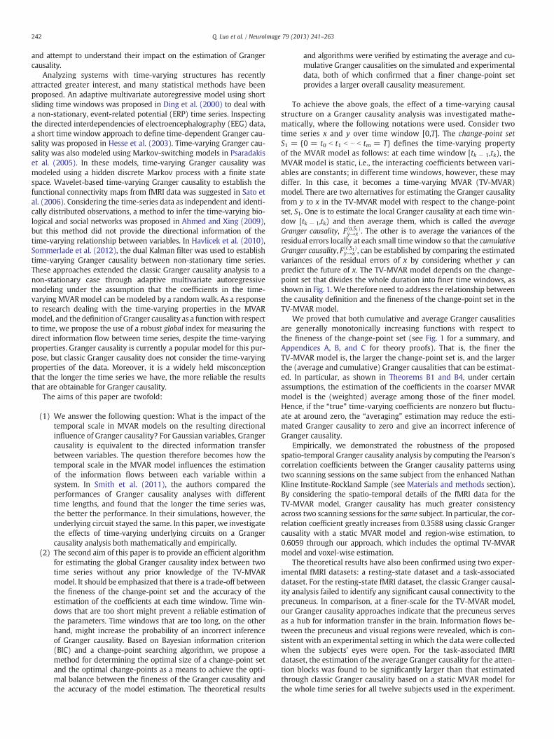
To achieve the above goals, the effect of a time-varying causalstructure on a Granger causality analysis was investigated mathe-matically, where the following notations were used. Consider twotime series x and y over time window [0,T]. The change-point setS1 = {0 = t0 b t1 b ⋯ b tm = T} defines the time-varying propertyof the MVAR model as follows: at each time window [tk − 1,tk), theMVAR model is static, i.e., the interacting coefficients between vari-ables are constants; in different time windows, however, these maydiffer. In this case, it becomes a time-varying MVAR (TV-MVAR)model. There are two alternatives for estimating the Granger causalityfrom y to x in the TV-MVAR model with respect to the change-pointset, S1. One is to estimate the local Granger causality at each time win-dow [tk − 1,tk) and then average them, which is called the averageGranger causality, F a;S1ð Þ

y→x . The other is to average the variances of theresidual errors locally at each small timewindow so that the cumulativeGranger causality, F c;S1ð Þ

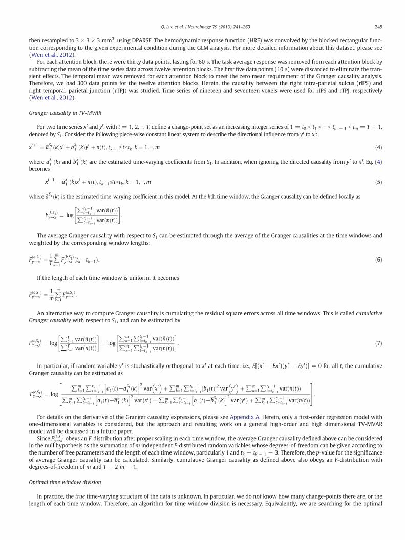
y→x , can be established by comparing the estimatedvariances of the residual errors of x by considering whether y canpredict the future of x. The TV-MVAR model depends on the change-point set that divides the whole duration into finer time windows, asshown in Fig. 1. We therefore need to address the relationship betweenthe causality definition and the fineness of the change-point set in theTV-MVAR model.

We proved that both cumulative and average Granger causalitiesare generally monotonically increasing functions with respect tothe fineness of the change-point set (see Fig. 1 for a summary, andAppendices A, B, and C for theory proofs). That is, the finer theTV-MVAR model is, the larger the change-point set is, and the largerthe (average and cumulative) Granger causalities that can be estimat-ed. In particular, as shown in Theorems B1 and B4, under certainassumptions, the estimation of the coefficients in the coarser MVARmodel is the (weighted) average among those of the finer model.Hence, if the “true” time-varying coefficients are nonzero but fluctu-ate at around zero, the “averaging” estimation may reduce the esti-mated Granger causality to zero and give an incorrect inference ofGranger causality.

Empirically, we demonstrated the robustness of the proposedspatio-temporal Granger causality analysis by computing the Pearson'scorrelation coefficients between the Granger causality patterns usingtwo scanning sessions on the same subject from the enhanced NathanKline Institute-Rockland Sample (see Materials and methods section).By considering the spatio-temporal details of the fMRI data for theTV-MVAR model, Granger causality has much greater consistencyacross two scanning sessions for the same subject. In particular, the cor-relation coefficient greatly increases from 0.3588 using classic Grangercausality with a static MVAR model and region-wise estimation, to0.6059 through our approach, which includes the optimal TV-MVARmodel and voxel-wise estimation.

The theoretical results have also been confirmed using two exper-imental fMRI datasets: a resting-state dataset and a task-associateddataset. For the resting-state fMRI dataset, the classic Granger causal-ity analysis failed to identify any significant causal connectivity to theprecuneus. In comparison, at a finer-scale for the TV-MVAR model,our Granger causality approaches indicate that the precuneus servesas a hub for information transfer in the brain. Information flows be-tween the precuneus and visual regions were revealed, which is con-sistent with an experimental setting in which the data were collectedwhen the subjects' eyes were open. For the task-associated fMRIdataset, the estimation of the average Granger causality for the atten-tion blocks was found to be significantly larger than that estimatedthrough classic Granger causality based on a static MVAR model forthe whole time series for all twelve subjects used in the experiment.

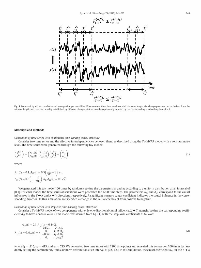
Fig. 1. Monotonicity of the cumulative and average Granger causalities. If we consider finer time windows with the same length, the change-point set can be derived from thewindow length, and thus the causality established by different change-point sets can be equivalently denoted by the corresponding window lengths mi for Si.

243Q. Luo et al. / NeuroImage 79 (2013) 241–263

Materials and methods

Generation of time series with continuous time-varying causal structureConsider two time series and the effective interdependencies between them, as described using the TV-MVAR model with a constant noise

level. The time series were generated through the following toy model:

xtþ1

ytþ1

� �¼ A11 tð Þ A12 tð Þ

A21 tð Þ A22 tð Þ� �

xt

yt

� �þ nt

xy

ntyx

!; ð1Þ

where

A11 tð Þ ¼ 0:1;A12 tð Þ ¼ 0:5t

600−1

� �⋅u1;

A21 tð Þ ¼ 0:5 1− t400

� �⋅u2;A22 tð Þ ¼ 0:1

ffiffiffi2

p:

We generated this toy model 100 times by randomly setting the parameters u1 and u2 according to a uniform distribution at an interval of[0,1]. For each model, the time series observations were generated for 1200 time steps. The parameters A12 and A21 correspond to the causalinfluences in the Y ➔ X and X ➔ Y directions, respectively. A significant nonzero causal coefficient indicates the causal influence in the corre-sponding direction. In this simulation, we specified a change in the causal coefficient from positive to negative.

Generation of time series with stepwise time-varying causal structureConsider a TV-MVAR model of two components with only one directional causal influence, X ➔ Y; namely, setting the corresponding coeffi-

cient A21 to have nonzero values. This model was derived from Eq. (1) with the step-wise coefficients as follows:

A11 tð Þ ¼ 0:1;A22 tð Þ ¼ 0:1ffiffiffi2

p;

A12 tð Þ ¼ 0;A21 tð Þ ¼0:5u1; 0bt≤t10; t1bt≤t2

−0:5u1; t2bt≤t30; t3bt≤T

8>><>>:ð2Þ

where t1 = 215, t2 = 415, and t3 = 715. We generated two time series with 1200 time points and repeated this generation 100 times by ran-domly setting the parameter u1 from a uniform distribution at an interval of [0.5, 1.5]. In this simulation, the causal coefficient A12 for the Y ➔ X

244 Q. Luo et al. / NeuroImage 79 (2013) 241–263

direction was set to zero, and thus there was no causal influence from Y to X, and the causal coefficient A21 varied across different timewindows.

Generation of BOLD signal with time-varying effective connectionHerein, we simulated the fMRI time series of two brain regions, X and Y, for 400 s. By introducing a time-varying causal structure, the

simulation scheme for the fMRI data in Schippers et al. (2011) was adopted. First, a neuronal interaction (local field potential, or LFP) wassimulated using a bi-dimensional first-order TV-MVAR model with a time step of 10 ms:

xtþ1

ytþ1

� �¼ A xt

yt

� �þ nt

xy

ntyx

!; ð3Þ

where

A11 ¼ 0:9;A22 ¼ 0:9;

A12 ¼ 0;A21 ¼ 0:5; 0bt≤18;000−0:5: 18;000bt≤40;000 :

�

The model had an causal influence from X to Y of a predetermined time-varying strength, A21, with no influence from Y to X.Second, both signalswere convolvedwith the default hemodynamic responsemodels from the SPM5 toolbox (http://www.fil.ion.ucl.ac.uk/spm/),

and Gaussian noises were added as physiological noise in the BOLD response. The HRF was specified through seven model parameters: delay ofresponse relative to onset (in seconds), delay of undershoot relative to onset (in seconds), dispersion of response, dispersion of undershoot, ratioof response to undershoot, onset (in seconds), and length of kernel. To investigate the effect of hemodynamic response variability on the Granger cau-sality analysis, we systematically varied the delay of response ranging from 0 to 5 s. To mimic the neuronal delay between the cause-region to theeffect-region, time series Y was shifted by 50 ms against X before the convolution of the HRF (Deshpande et al., 2010; Schippers et al., 2011; Smithet al., 2012).

Third, BOLD signals were generated by down-sampling the convolved time series by 2 Hz as a high sampling rate, and 1 Hz as a low samplingrate (resembling an acquisition rate (TR) of an MR-scanner), and Gaussian noise was again added as acquisition noise. After each step, the sig-nals were normalized to zero means and unit variances. The total amount of noise added was 20%.

Multiband Imaging test–retest pilot datasetThis set of fMRI data comes from the enhanced Nathan Kline Institute-Rockland Sample. The whole dataset consists of resting-state fMRI

recordings from two sessions for seventeen subjects (healthy, aged 19–57, thirteen males and four females).The fMRI data were collected using 3 T, and 40 slices were acquired for 900 volumes. Multiband echo planar imaging approaches enable the

acquisition of fMRI data with unprecedented sampling rates (TR = 0.645 s) for full-brain coverage through an acquisition of multiple slices si-multaneously at the same time. For more detailed information about this dataset, please see the website at http://fcon_1000.projects.nitrc.org/indi/pro/eNKI_RS_TRT/FrontPage.html.

Data pre-processing was performed using DPARSF software (Yan and Zang, 2010). The first fifty volumes were discarded to allow for scannerstabilization. Since multiple slices were excited simultaneously, a simple slice time correction might not work well. Given its short effective TR,such a correction is probably less important, and is therefore omitted in our data pre-processing. After the realignment for head-motion correc-tion, the standard Montreal Neurological Institute (MNI) template provided by SPM2 was used for spatial normalization with a re-samplingvoxel size of 3 × 3 × 3 mm3. After smoothing (FWHM = 8 mm), the imaging data were temporally filtered (band pass, 0.01–0.08 Hz) toremove the effects of a very low-frequency drift and high-frequency noises (e.g., respiratory and cardiac rhythms). An automated anatomicallabeling (AAL) atlas (Tzourio-Mazoyer et al., 2002) was used to parcellate the brain into ninety regions of interest (ROIs). To verify the principleof voxel-level Granger causality, the brain was also divided into 1024 ROIs with around 45 voxels each according to a high-resolution brain atlasprovided by Zalesky et al. (2010).

Resting-state fMRI datasetThe resting-state fMRI dataset is a subset of a large database, called the 1000 Functional Connectomes Project (Biswal et al., 2010),

which is freely accessible at www.nitrc.org/projects/fcon_1000/. The dataset provided by Buckner's group at Cambridge, USA, was usedfor the present study. This dataset consists of 198 healthy subjects (75 males and 123 females, aged 18–30). The fMRI data (TR = 3 s)were collected using 3 T, and 47 slices were acquired for 119 volumes. Further details about this dataset can be found at the websiteprovided above.

The first five volumes were discarded to allow for scanner stabilization. DPARSF (Yan and Zang, 2010), which is based on SPM8, was used forpre-processing the fMRI data, including slice-timing correction, motion correction, co-registration, gray/white matter segmentation, and spatialnormalization into a Montreal Neurological Institute (MNI) space, then and re-sampled to 3 × 3 × 3 mm3. The waveform of each voxel wasdetrended and passed through a band-pass filter of 0.01 to 0.08 Hz. The data were smoothed spatially (FWHM = 8 mm). As a result, time seriesdata with 114 time points from ninety brain regions (AAL-atlas) for 198 subjects were achieved.

fMRI dataset for attention taskThe dataset of an fMRI time series for an attention-task experiment was provided by the Ding Group at the University of Florida, USA (Wen et

al., 2012), which consisted of twelve subjects who successfully completed the task (eight females and four males, aged 20–28). This experimentadopted a mixed blocked/event-related design. There were twelve attention blocks and twelve passive-view blocks, along with some fixationintervals. In each attention block, the subjects performed a trial-by-trail cued visual spatial-attention task. The fMRI data were collected using3 T, and 33 slices were acquired for 180 volumes for each of the six runs with TR 2 s. The dataset was pre-processed by slice timing, motioncorrection, co-registration to an individual anatomical image, and normalization to the Montreal Neurological Institute (MNI) template, and

245Q. Luo et al. / NeuroImage 79 (2013) 241–263

then resampled to 3 × 3 × 3 mm3, using DPARSF. The hemodynamic response function (HRF) was convolved by the blocked rectangular func-tion corresponding to the given experimental condition during the GLM analysis. For more detailed information about this dataset, please see(Wen et al., 2012).

For each attention block, there were thirty data points, lasting for 60 s. The task average response was removed from each attention block bysubtracting the mean of the time series data across twelve attention blocks. The first five data points (10 s) were discarded to eliminate the tran-sient effects. The temporal mean was removed for each attention block to meet the zero mean requirement of the Granger causality analysis.Therefore, we had 300 data points for the twelve attention blocks. Herein, the causality between the right intra-parietal sulcus (rIPS) andright temporal–parietal junction (rTPJ) was studied. Time series of nineteen and seventeen voxels were used for rIPS and rTPJ, respectively(Wen et al., 2012).

Granger causality in TV-MVAR

For two time series xt and yt, with t = 1, 2, ⋯, T, define a change-point set as an increasing integer series of 1 = t0 b t1 b ⋯ b tm − 1 b tm = T + 1,denoted by S1. Consider the following piece-wise constant linear system to describe the directional influence from yt to xt:

xtþ1 ¼ aS11 kð Þxt þ bS1

1 kð Þyt þ n tð Þ; tk−1≤tbtk; k ¼ 1; ⋯;m ð4Þ

where aS11 kð Þ and bS1

1 kð Þ are the estimated time-varying coefficients from S1. In addition, when ignoring the directed causality from yt to xt, Eq. (4)becomes

xtþ1 ¼ ~aS11 kð Þxt þ ~n tð Þ; tk−1≤tbtk; k ¼ 1; ⋯;m ð5Þ

where ~aS11 kð Þ is the estimated time-varying coefficient in this model. At the kth time window, the Granger causality can be defined locally as

F k;S1ð Þy→x ¼ log

∑tk−1t¼tk−1

var ~n tð Þð Þ∑tk−1

t¼tk−1var n tð Þð Þ

" #:

The average Granger causality with respect to S1 can be estimated through the average of the Granger causalities at the time windows andweighted by the corresponding window lengths:

F a;S1ð Þy→x ¼ 1

T∑m

k¼1F k;S1ð Þy→x tk−tk−1ð Þ: ð6Þ

If the length of each time window is uniform, it becomes

F a;S1ð Þy→x ¼ 1

m∑m

k¼1F k;S1ð Þy→x :

An alternative way to compute Granger causality is cumulating the residual square errors across all time windows. This is called cumulativeGranger causality with respect to S1, and can be estimated by

F c;S1ð ÞY→X ¼ log

∑Tt¼1 var ~n tð Þð Þ

∑Tt¼1 var n tð Þð Þ

" #¼ log

∑mk¼1∑

tk−1t¼tk−1

var ~n tð Þð Þ∑m

k¼1∑tk−1t¼tk−1

var n tð Þð Þ

" #: ð7Þ

In particular, if random variable yt is stochastically orthogonal to xt at each time, i.e., E[(xt − Ext)(yt − Eyt)] = 0 for all t, the cumulativeGranger causality can be estimated as

F c;S1ð ÞY→X ¼ log

∑mk¼1∑

tk−1t¼tk−1

a1 tð Þ−~aS11 kð Þ

h i2var xt� �

þ∑mk¼1∑

tk−1t¼tk−1

b1 tð Þ½ �2 var yt� �

þ∑mk¼1∑

tk−1t¼tk−1

var n tð Þð Þ

∑mk¼1∑

tk−1t¼tk−1

a1 tð Þ−aS11 kð Þ

h i2var xt� þ∑m

k¼1∑tk−1t¼tk−1

b1 tð Þ−bS11 kð Þ

h i2var yt� þ∑m

k¼1∑tk−1t¼tk−1

var n tð Þð Þ

264375:

For details on the derivative of the Granger causality expressions, please see Appendix A. Herein, only a first-order regression model withone-dimensional variables is considered, but the approach and resulting work on a general high-order and high dimensional TV-MVARmodel will be discussed in a future paper.

Since F k;S1ð Þy→x obeys an F-distribution after proper scaling in each time window, the average Granger causality defined above can be considered

in the null hypothesis as the summation ofm independent F-distributed random variables whose degrees-of-freedom can be given according tothe number of free parameters and the length of each time window, particularly 1 and tk − tk − 1 − 3. Therefore, the p-value for the significanceof average Granger causality can be calculated. Similarly, cumulative Granger causality as defined above also obeys an F-distribution withdegrees-of-freedom of m and T − 2 m − 1.

Optimal time window division

In practice, the true time-varying structure of the data is unknown. In particular, we do not know how many change-points there are, or thelength of each time window. Therefore, an algorithm for time-window division is necessary. Equivalently, we are searching for the optimal

246 Q. Luo et al. / NeuroImage 79 (2013) 241–263

change-point set. The optimal time-window division indicates a trade-off between the satisfactory accuracy of the model parameter estimationand the lossless causal information established by the model. Mathematically, consider the following step-wise TV-MVAR model

X t þ 1ð Þ ¼Xmk¼1

ak1X tð ÞI tk−1 ;tk½ Þ þ n tð Þ; ð8Þ

where I tk−1 ;tk½ � is the characteristic function of time window [tk − 1,tk), n(t) is a Gaussian white noise term, a1k represents a (constant) coefficient inthe kth interval, and

S mð Þ ¼ t1; ⋯; tm−1 1 ¼ t0bt1b⋯btm−1btm ¼ T þ 1j gf

is the change-point set. Given the change-points, the model can be fit into each time window as ak1, and the variance of the residual errors can be

estimated for each time window, denoted by Σk. Therefore, the accuracy of the model can be defined based on the weighted average of thevariances of the residuals in each time window as follows:

err S mð Þð Þ ¼ 1m

Xmk¼1

tk−tk−1ð Þdet Σk

� �: ð9Þ

On the other hand, the information captured by this model can be measured based on the average Granger causality in all directions definedin the previous section, as noted by

agc S mð Þð Þ ¼ 12m

Xmk¼1

F k;S mð Þð Þy→x þ F k;S mð Þð Þ

x→y

� �: ð10Þ

To minimize the prediction error and maximize the detected causality information, the optimal window division can be derived by optimiz-ing the following cost function with the trade-off parameter λ

Sopt m;λð Þ ¼ argminS mð Þ

err S mð Þð Þ þ λ=agc S mð Þð Þð Þ: ð11Þ

Given the trade-off parameter λ0 and lower bound l0 of the lengths of the divided time windows, the optimal change-points SOpt(m,λ0) can beestablished by solving the following constrained optimization problem

minS mð Þ err S mð Þð Þ þ λ0=agc S mð Þð Þð Þs:t: tk−tk−1≥l0 for allk ¼ 1;2;…;m:

ð12Þ

A constrained condition is required for a reliable estimation of the model coefficients in Eq. (8) at each divided time window. Thisconstrained optimization problem can be solved based on the optimization functions provided in MATLAB. In this paper, we used the fminconfunction for a nonlinear constrained optimization problem.

To determine the parameter, we search for the optimal change-point set Sopt(m,λ) for different λ ∈ [λ1,λ2], and then calculate the Bayesianinformation criterion (BIC) for this change-point set as follows:

BIC m;λð Þ ¼ −2Xmk¼1

LLFk þ 22m log T þ 1ð Þ; ð13Þ

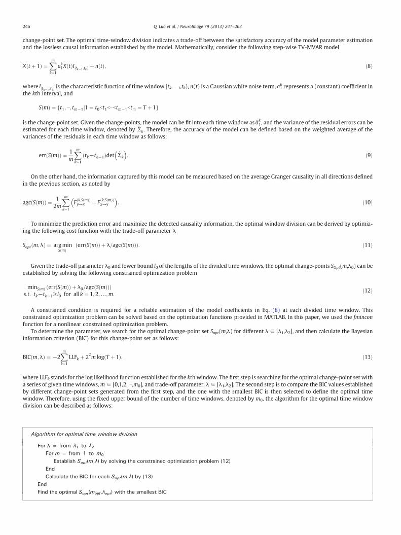
where LLFk stands for the log likelihood function established for the kth window. The first step is searching for the optimal change-point set witha series of given time windows,m ∈ [0,1,2, ⋯,m0], and trade-off parameter, λ ∈ [λ1,λ2]. The second step is to compare the BIC values establishedby different change-point sets generated from the first step, and the one with the smallest BIC is then selected to define the optimal timewindow. Therefore, using the fixed upper bound of the number of time windows, denoted by m0, the algorithm for the optimal time windowdivision can be described as follows:

Algorithm for optimal time window division

For λ = from λ1 to λ2For m = from 1 to m0

Establish Sopt(m,λ) by solving the constrained optimization problem (12)EndCalculate the BIC for each Sopt(m,λ) by (13)

EndFind the optimal Sopt(mopt,λopt) with the smallest BIC

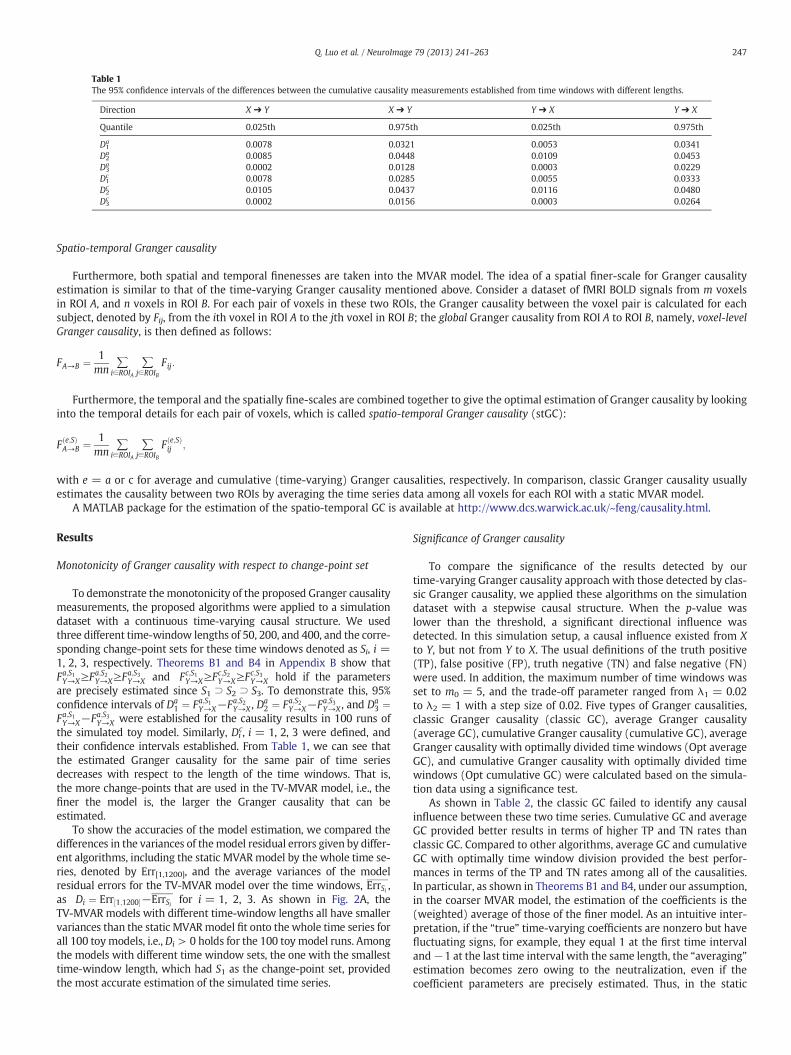
Table 1The 95% confidence intervals of the differences between the cumulative causality measurements established from time windows with different lengths.

Direction X ➔ Y X ➔ Y Y ➔ X Y ➔ X

Quantile 0.025th 0.975th 0.025th 0.975th

D1a 0.0078 0.0321 0.0053 0.0341

D2a 0.0085 0.0448 0.0109 0.0453

D3a 0.0002 0.0128 0.0003 0.0229

D1c 0.0078 0.0285 0.0055 0.0333

D2c 0.0105 0.0437 0.0116 0.0480

D3c 0.0002 0.0156 0.0003 0.0264

247Q. Luo et al. / NeuroImage 79 (2013) 241–263

Spatio-temporal Granger causality

Furthermore, both spatial and temporal finenesses are taken into the MVAR model. The idea of a spatial finer-scale for Granger causalityestimation is similar to that of the time-varying Granger causality mentioned above. Consider a dataset of fMRI BOLD signals from m voxelsin ROI A, and n voxels in ROI B. For each pair of voxels in these two ROIs, the Granger causality between the voxel pair is calculated for eachsubject, denoted by Fij, from the ith voxel in ROI A to the jth voxel in ROI B; the global Granger causality from ROI A to ROI B, namely, voxel-levelGranger causality, is then defined as follows:

FA→B ¼ 1mn

∑i∈ROIA

∑j∈ROIB

Fij:

Furthermore, the temporal and the spatially fine-scales are combined together to give the optimal estimation of Granger causality by lookinginto the temporal details for each pair of voxels, which is called spatio-temporal Granger causality (stGC):

F e;Sð ÞA→B ¼ 1

mn∑

i∈ROIA∑

j∈ROIBF e;Sð Þij ;

with e = a or c for average and cumulative (time-varying) Granger causalities, respectively. In comparison, classic Granger causality usuallyestimates the causality between two ROIs by averaging the time series data among all voxels for each ROI with a static MVAR model.

A MATLAB package for the estimation of the spatio-temporal GC is available at http://www.dcs.warwick.ac.uk/~feng/causality.html.

Results

Monotonicity of Granger causality with respect to change-point set

To demonstrate themonotonicity of the proposed Granger causalitymeasurements, the proposed algorithms were applied to a simulationdataset with a continuous time-varying causal structure. We usedthree different time-window lengths of 50, 200, and 400, and the corre-sponding change-point sets for these time windows denoted as Si, i =1, 2, 3, respectively. Theorems B1 and B4 in Appendix B show thatFa;S1Y→X≥Fa;S2Y→X≥Fa;S3Y→X and Fc;S1Y→X≥Fc;S2Y→X≥Fc;S3Y→X hold if the parametersare precisely estimated since S1 ⊃ S2 ⊃ S3. To demonstrate this, 95%confidence intervals of Da

1 ¼ Fa;S1Y→X−Fa;S2Y→X , Da2 ¼ Fa;S2Y→X−Fa;S3Y→X , and Da

3 ¼Fa;S1Y→X−Fa;S3Y→X were established for the causality results in 100 runs ofthe simulated toy model. Similarly, Di

c, i = 1, 2, 3 were defined, andtheir confidence intervals established. From Table 1, we can see thatthe estimated Granger causality for the same pair of time seriesdecreases with respect to the length of the time windows. That is,the more change-points that are used in the TV-MVAR model, i.e., thefiner the model is, the larger the Granger causality that can beestimated.

To show the accuracies of the model estimation, we compared thedifferences in the variances of themodel residual errors given by differ-ent algorithms, including the static MVARmodel by the whole time se-ries, denoted by Err[1,1200], and the average variances of the modelresidual errors for the TV-MVAR model over the time windows, ErrSi ,as Di ¼ Err 1;1200½ �−ErrSi for i = 1, 2, 3. As shown in Fig. 2A, theTV-MVAR models with different time-window lengths all have smallervariances than the static MVARmodel fit onto the whole time series forall 100 toymodels, i.e., Di > 0 holds for the 100 toy model runs. Amongthe models with different time window sets, the one with the smallesttime-window length, which had S1 as the change-point set, providedthe most accurate estimation of the simulated time series.

Significance of Granger causality

To compare the significance of the results detected by ourtime-varying Granger causality approach with those detected by clas-sic Granger causality, we applied these algorithms on the simulationdataset with a stepwise causal structure. When the p-value waslower than the threshold, a significant directional influence wasdetected. In this simulation setup, a causal influence existed from Xto Y, but not from Y to X. The usual definitions of the truth positive(TP), false positive (FP), truth negative (TN) and false negative (FN)were used. In addition, the maximum number of time windows wasset to m0 = 5, and the trade-off parameter ranged from λ1 = 0.02to λ2 = 1 with a step size of 0.02. Five types of Granger causalities,classic Granger causality (classic GC), average Granger causality(average GC), cumulative Granger causality (cumulative GC), averageGranger causality with optimally divided time windows (Opt averageGC), and cumulative Granger causality with optimally divided timewindows (Opt cumulative GC) were calculated based on the simula-tion data using a significance test.

As shown in Table 2, the classic GC failed to identify any causalinfluence between these two time series. Cumulative GC and averageGC provided better results in terms of higher TP and TN rates thanclassic GC. Compared to other algorithms, average GC and cumulativeGC with optimally time window division provided the best perfor-mances in terms of the TP and TN rates among all of the causalities.In particular, as shown in Theorems B1 and B4, under our assumption,in the coarser MVAR model, the estimation of the coefficients is the(weighted) average of those of the finer model. As an intuitive inter-pretation, if the “true” time-varying coefficients are nonzero but havefluctuating signs, for example, they equal 1 at the first time intervaland−1 at the last time interval with the same length, the “averaging”estimation becomes zero owing to the neutralization, even if thecoefficient parameters are precisely estimated. Thus, in the static

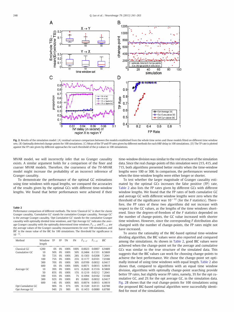
Fig. 2. Results of the simulation model: (A) residual variance comparison between the models established from the whole time series and those models fitted on different time windowsets. (B) Optimally detected change-points for 100 simulations. (C)Mean of the TP and FP rates given by differentmethods for eachHRF delay in 100 simulations. (D) The TP rate is plottedagainst the FP rate given by different approaches for each threshold of the p-values in 100 simulations.

248 Q. Luo et al. / NeuroImage 79 (2013) 241–263

MVAR model, we will incorrectly infer that no Granger causalityexists. A similar argument holds for a comparison of the finer andcoarser MVAR models. Therefore, the coarseness of the TV-MVARmodel might increase the probability of an incorrect inference ofGranger causality.

To demonstrate the performance of the optimal GC estimationsusing time windows with equal lengths, we compared the accuraciesof the results given by the optimal GCs with different time-windowlengths. We found that better performances were achieved if their

Table 2Performance comparison of different methods. The term ‘Classical GC’ is short for classicGranger causality, ‘Cumulative GC’ stands for cumulative Granger causality, ‘Average GC’is the average Granger causality, ‘Opt Cumulative GC’ stands for the cumulative Grangercausality with optimally divided time windows, and ‘Opt Average GC’ indicates the aver-age Granger causality with the optimally determined time windows. F X→Y and F Y→X arethe average values of the Granger causality measurements for over 100 simulations, andBIC is the mean value of the BIC for 100 simulations. The threshold for significance is10−12.

Method Windowlength

TP FP TN FN F X→Y F Y→X BIC

Classical GC 1200 0% 0% 100% 100% 0.0023 0.0007 6.9489Cumulative GC 10 50% 0% 100% 50% 0.2484 0.1331 8.5869

50 72% 0% 100% 28% 0.1303 0.0208 7.2041100 75% 0% 100% 25% 0.1177 0.0101 7.0188300 70% 0% 100% 30% 0.0709 0.0032 6.9417600 0% 0% 100% 100% 0.0071 0.0015 6.9819

Average GC 10 39% 0% 100% 61% 0.2620 0.1516 8.586950 85% 0% 100% 15% 0.1219 0.0212 7.2041

100 93% 0% 100% 7% 0.1094 0.0102 7.0188300 92% 0% 100% 8% 0.0681 0.0032 6.9417600 14% 0% 100% 86% 0.0074 0.0015 6.9819

Opt Cumulative GC 90% 3% 97% 10% 0.1320 0.0131 6.8780Opt Average GC 94% 2% 98% 6% 0.1453 0.0080 6.8780

time-windowdivisionwas similar to the real structure of the simulationdata. Since the real change-points of this simulation were 215, 415, and715, both algorithms presented better results when the time-windowlengths were 100 or 300. In comparison, the performances worsenedwhen the time-window lengths were either longer or shorter.

To test whether the larger magnitude of Granger causality esti-mated by the optimal GCs increases the false positive (FP) rate,Table 2 also lists the FP rates given by different GCs with differentwindow lengths. We found that the FP rates of both cumulative GCand average GC with different window lengths were zero when thethreshold of the significance was 10−12 (for the F statistics). There-fore, the FP rates of these two algorithms did not increase withrespect to the GC values, as the lengths of the time windows short-ened. Since the degrees-of-freedom of the F statistics depended onthe number of change-points, the GC value increased with shortertime windows. However, since the corresponding F distribution alsochanged with the number of change-points, the FP rates might nothave increased.

To assess the rationality of the BIC-based optimal time-windowdividing algorithm, the BIC values were also reported and comparedamong the simulations. As shown in Table 2, good BIC values wereachieved when the change-point set for the average and cumulativeGCs was similar to the true structure of the simulated data. Thissuggests that the BIC values can work for choosing change-points toachieve the best performance. We chose the change-point set opti-mally instead of using time windows with equal length. Table 2 alsoshows that, compared to algorithms with an equal time windowdivision, algorithms with optimally change-point searching providebetter TP rates, but slightly worse FP rates, namely, 3% for the opt cu-mulative GC, and 2% for the opt average GC, in the simulation data.Fig. 2B shows that the real change-points for 100 simulations usingthe proposed BIC-based optimal algorithm were successfully identi-fied for most of the simulations.

249Q. Luo et al. / NeuroImage 79 (2013) 241–263

To compare the computational complexities among the different al-gorithms, we reported the running time of each algorithm on the simu-lated dataset. As listed in Table 3, because the method for optimallydividing the time windows is very time-consuming, the greater thenumber of time windows we used, the greater the amount of timethat was required to run the algorithm. In practice, since the underlyingtime-varying structure of the data is unknown,we can either run the op-timal time-window dividing algorithm, or try different time-windowlengths and select the optimal length through a comparison of their BICs.

Effect of regional variation in HRF on Granger causality analysis

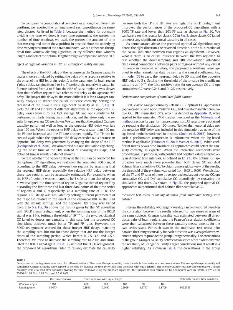
The effects of the HRF delay of the response on the Granger causalityanalysis were simulated by setting the delay of the response relative tothe onset of the HRF for brain region X as the parameter for brain regionY plus a delay ranging from 0 to 3 s. Therefore, the underlying causal in-fluence existed from X to Y, but the HRF of cause-region X was slowerthan that of effect-region Y. We refer to this delay as the opposite HRFdelay. The longer this delay is, the more difficult it is for a Granger cau-sality analysis to detect the causal influence correctly. Setting thethreshold of the p-value for a significant causality as 10−6, Fig. 2Cplots the TP and FP rates of different algorithms as the opposite HRFdelay varies from 0 to 3 s. Opt average GC and opt cumulative GCperformed similarly during the simulation, and therefore, only the re-sults for opt average GC are shown.We can see that the optimal Grangercausality performed well as long as the opposite HRF delay was lessthan 100 ms. When the opposite HRF delay was greater than 100 ms,the FP rate increased and the TP rate dropped rapidly. The TP rate in-creased again when the opposite HRF delay exceeded 0.4 s because anopposite HRF delay was generated by changing the shape of the HRF(Deshpande et al., 2010).We also carried out our simulations by chang-ing the onset time of the HRF instead of changing its shape, andobtained similar results (data not shown).

To test whether the opposite delay in the HRF can be corrected forthe optimal GC algorithms, we realigned the simulated BOLD signalaccording to the HRF delay between two regions by assuming thatthe regional HRF delay, especially the relative HRF delay betweenthese two regions, can be accurately estimated. For example, whenthe HRF of region Y was estimated to be 3 s faster than that of regionX, we realigned the time series of region X against that of region Y bydiscarding the first three and last three data points of the time seriesof regions X and Y, respectively, at a sampling rate of 1 Hz. Theregional HRF delay was simulated by setting different parameters ofthe response relative to the onset in the canonical HRF in the SPMwith the default settings, and the opposite HRF delay was variedfrom 2 to 5 s. Fig. 3A shows the results given by the GC algorithmwith BOLD signal realignment, when the sampling rate of the BOLDsignal was 1 Hz. Setting a threshold of 10−9 for the p-value, classicalGC failed to detect any causality in this case, but the proposed GCalgorithms achieved much better TP and FP rates. However, theBOLD realignment worked for those integer HRF delays matchingthe sampling rate, but not for those delays that are not the integertimes of the sampling period, which herein is 2.5, 3.5, and 4.5 s.Therefore, we tried to increase the sampling rate to 2 Hz, and simu-lated the BOLD signal again. In Fig. 3B, without the BOLD realignment,the proposed GC algorithms failed to reliably estimate the causality

Table 3Comparison of running time (in seconds) for different methods. The classic Granger causalitcumulative Granger causality were applied to the data by dividing the time series into timcausality were also used after optimally dividing the time windows using the proposed alT5600 @ 1.83 GHz, 1.83 GHz, and 1.5 G RAM.

One time window Time windows with equal lengt

Window length 1200 600 300Running time 0.0073 0.2936 0.4697

because both the TP and FP rates are high. The BOLD realignmentimproved the performances of the proposed GC algorithms with a100% TP rate and lower than 20% FP rate, as shown in Fig. 3C. Wecan barely see the results for classic GC in Fig. 3, since classic GC failedto detect any significant causal causality in all cases.

As demonstrated above, the proposed optimal GC algorithms maydetect the right direction, the reversed direction, or the bi-direction ofthe causal influence between two regions as significant. However,what if there is no causal influence between the two regions? Totest whether the downsampling and HRF convolution introducefalse causal connections between pairs of regions without any causalinfluence in neuronal activities, the proposed algorithms were ap-plied to other simulation data by setting the causal coefficient, A21,in model (3) to zero, the neuronal delay to 50 ms, and the oppositeHRF delay to 3 s. Setting the threshold of the p-value for significantcausality as 10−6, the false positive rates for opt average GC and optcumulative GC were 0.24% and 0.12%, respectively.

Performance comparison of simulated fMRI dataset

First, classic Granger causality (classic GC), optimal GC approaches(opt average GC and opt cumulative GC), and dual Kalman filter cumula-tive GC (Dkf cumulative GC), which is defined in Appendix D, wereapplied to the simulated fMRI dataset described in the Materials andmethods section for a performance comparison. All resultswere obtainedby repeating the simulation 100 times. Neither the neuronal delay northe negative HRF delay was included in this simulation, as none of thelag-based methods work well in this case (Smith et al., 2012); however,such a performance comparison is informative when the lag-basedmethod is applicable (Friston et al., 2012; Wen et al., 2012). When coef-ficient matrix Awas time-invariant, all approaches could detect the cau-sality correctly, as expected. When the interaction coefficients weretime-varying, in particular, with positive and negative values alternative-ly in different time intervals, as defined in Eq. (3), the optimal GC ap-proaches were much more powerful than both classic GC and dualKalman filter cumulative GC. To obtain a more global view of the results,the threshold of the p-values was varied from 0.05 to 0.001.We calculat-ed the TP and FP rates of these three approaches, i.e., opt average GC, optcumulative GC, and Dkf cumulative GC, accordingly, by repeating thesimulation 100 times. As shown in Fig. 2D, the proposed optimal GCapproaches outperformed dual Kalman filter cumulative GC.

Increased test–retest reliability obtained from multiband resting-statedataset

Herein, the reliability of Granger causality can bemeasured based onthe correlation between the results inferred for two series of scans ofthe same subjects. Granger causality was estimated between all direc-tional pairs of brain regions, and the Pearson's correlation coefficientswere then calculated between these causality measurements for thetwo series scans. For each scan in the multiband test–retest pilotdataset, the Granger causality for each directionwas averaged over sev-enteen subjects to provide the groupGranger causality. The correlationsof the groupGranger causality between two series of scans demonstratethe reliability of Granger causality. Larger correlations might result in ahigher reliability. As shown in Fig. 4, the correlations in the group

y treats the whole time series as a one time window. The average Granger causality ande windows with equal lengths. The average Granger causality and cumulative Grangergorithm. This simulation was carried out by a computer with an Intel® Core™ 2 CPU

h Optimally divided time windows

100 50 100.9969 1.9747 9.8709 346.5863

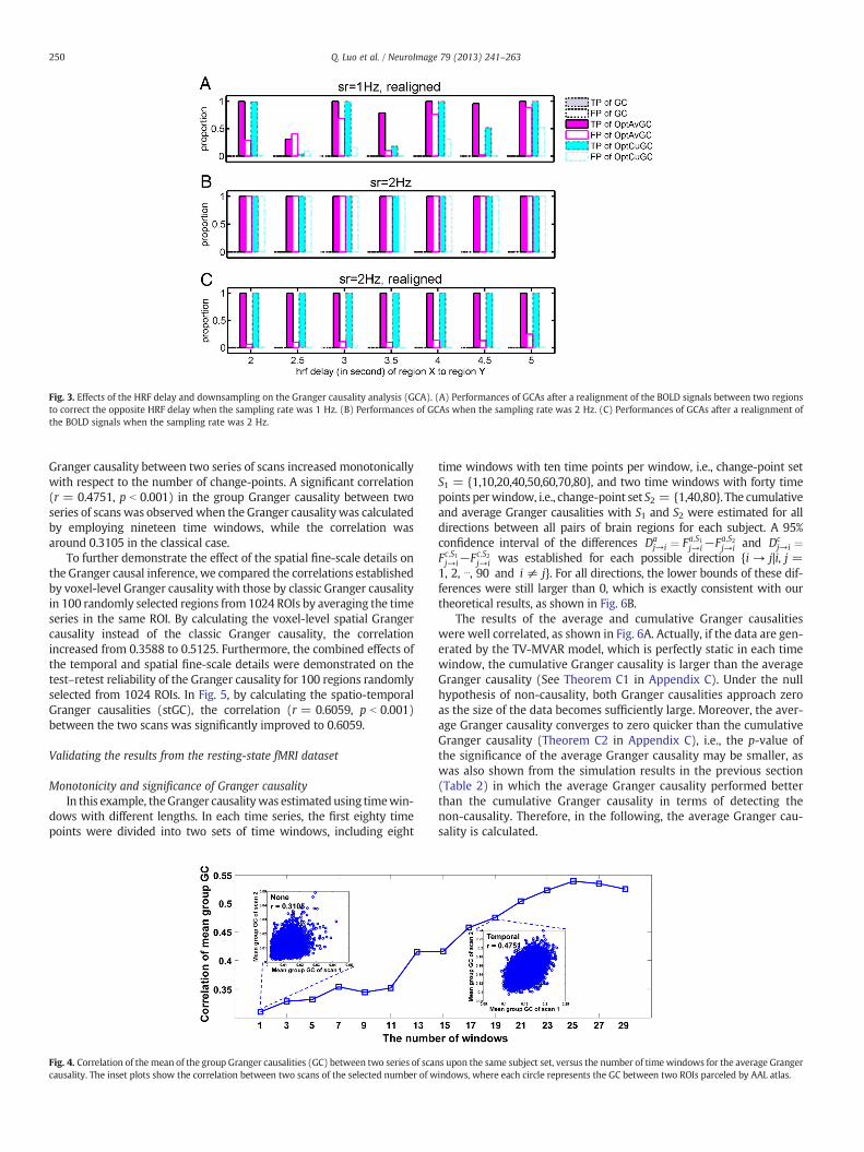
Fig. 3. Effects of the HRF delay and downsampling on the Granger causality analysis (GCA). (A) Performances of GCAs after a realignment of the BOLD signals between two regionsto correct the opposite HRF delay when the sampling rate was 1 Hz. (B) Performances of GCAs when the sampling rate was 2 Hz. (C) Performances of GCAs after a realignment ofthe BOLD signals when the sampling rate was 2 Hz.

250 Q. Luo et al. / NeuroImage 79 (2013) 241–263

Granger causality between two series of scans increased monotonicallywith respect to the number of change-points. A significant correlation(r = 0.4751, p b 0.001) in the group Granger causality between twoseries of scans was observedwhen the Granger causalitywas calculatedby employing nineteen time windows, while the correlation wasaround 0.3105 in the classical case.

To further demonstrate the effect of the spatial fine-scale details onthe Granger causal inference, we compared the correlations establishedby voxel-level Granger causality with those by classic Granger causalityin 100 randomly selected regions from 1024 ROIs by averaging the timeseries in the same ROI. By calculating the voxel-level spatial Grangercausality instead of the classic Granger causality, the correlationincreased from 0.3588 to 0.5125. Furthermore, the combined effects ofthe temporal and spatial fine-scale details were demonstrated on thetest–retest reliability of the Granger causality for 100 regions randomlyselected from 1024 ROIs. In Fig. 5, by calculating the spatio-temporalGranger causalities (stGC), the correlation (r = 0.6059, p b 0.001)between the two scans was significantly improved to 0.6059.

Validating the results from the resting-state fMRI dataset

Monotonicity and significance of Granger causalityIn this example, theGranger causalitywas estimated using timewin-

dows with different lengths. In each time series, the first eighty timepoints were divided into two sets of time windows, including eight

Fig. 4. Correlation of the mean of the group Granger causalities (GC) between two series of scacausality. The inset plots show the correlation between two scans of the selected number of w

time windows with ten time points per window, i.e., change-point setS1 = {1,10,20,40,50,60,70,80}, and two time windows with forty timepoints perwindow, i.e., change-point set S2 = {1,40,80}. The cumulativeand average Granger causalities with S1 and S2 were estimated for alldirections between all pairs of brain regions for each subject. A 95%confidence interval of the differences Da

j→i ¼ Fa;S1j→i−Fa;S2j→i and Dcj→i ¼

Fc;S1j→i−Fc;S2j→i was established for each possible direction {i → j|i, j =1, 2, ⋯, 90 and i ≠ j}. For all directions, the lower bounds of these dif-ferences were still larger than 0, which is exactly consistent with ourtheoretical results, as shown in Fig. 6B.

The results of the average and cumulative Granger causalitieswere well correlated, as shown in Fig. 6A. Actually, if the data are gen-erated by the TV-MVAR model, which is perfectly static in each timewindow, the cumulative Granger causality is larger than the averageGranger causality (See Theorem C1 in Appendix C). Under the nullhypothesis of non-causality, both Granger causalities approach zeroas the size of the data becomes sufficiently large. Moreover, the aver-age Granger causality converges to zero quicker than the cumulativeGranger causality (Theorem C2 in Appendix C), i.e., the p-value ofthe significance of the average Granger causality may be smaller, aswas also shown from the simulation results in the previous section(Table 2) in which the average Granger causality performed betterthan the cumulative Granger causality in terms of detecting thenon-causality. Therefore, in the following, the average Granger cau-sality is calculated.

ns upon the same subject set, versus the number of time windows for the average Grangerindows, where each circle represents the GC between two ROIs parceled by AAL atlas.

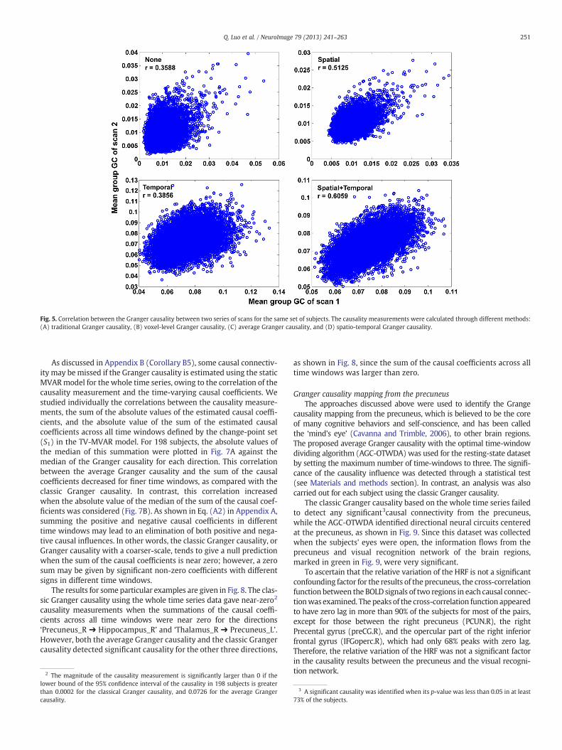
Fig. 5. Correlation between the Granger causality between two series of scans for the same set of subjects. The causality measurements were calculated through different methods:(A) traditional Granger causality, (B) voxel-level Granger causality, (C) average Granger causality, and (D) spatio-temporal Granger causality.

251Q. Luo et al. / NeuroImage 79 (2013) 241–263

As discussed in Appendix B (Corollary B5), some causal connectiv-ity may bemissed if the Granger causality is estimated using the staticMVARmodel for the whole time series, owing to the correlation of thecausality measurement and the time-varying causal coefficients. Westudied individually the correlations between the causality measure-ments, the sum of the absolute values of the estimated causal coeffi-cients, and the absolute value of the sum of the estimated causalcoefficients across all time windows defined by the change-point set(S1) in the TV-MVAR model. For 198 subjects, the absolute values ofthe median of this summation were plotted in Fig. 7A against themedian of the Granger causality for each direction. This correlationbetween the average Granger causality and the sum of the causalcoefficients decreased for finer time windows, as compared with theclassic Granger causality. In contrast, this correlation increasedwhen the absolute value of the median of the sum of the causal coef-ficients was considered (Fig. 7B). As shown in Eq. (A2) in Appendix A,summing the positive and negative causal coefficients in differenttime windows may lead to an elimination of both positive and nega-tive causal influences. In other words, the classic Granger causality, orGranger causality with a coarser-scale, tends to give a null predictionwhen the sum of the causal coefficients is near zero; however, a zerosum may be given by significant non-zero coefficients with differentsigns in different time windows.

The results for some particular examples are given in Fig. 8. The clas-sic Granger causality using the whole time series data gave near-zero2

causality measurements when the summations of the causal coeffi-cients across all time windows were near zero for the directions‘Precuneus_R ➔ Hippocampus_R’ and ‘Thalamus_R ➔ Precuneus_L’.However, both the average Granger causality and the classic Grangercausality detected significant causality for the other three directions,

2 The magnitude of the causality measurement is significantly larger than 0 if thelower bound of the 95% confidence interval of the causality in 198 subjects is greaterthan 0.0002 for the classical Granger causality, and 0.0726 for the average Grangercausality.

as shown in Fig. 8, since the sum of the causal coefficients across alltime windows was larger than zero.

Granger causality mapping from the precuneusThe approaches discussed above were used to identify the Grange

causality mapping from the precuneus, which is believed to be the coreof many cognitive behaviors and self-conscience, and has been calledthe ‘mind's eye’ (Cavanna and Trimble, 2006), to other brain regions.The proposed average Granger causality with the optimal time-windowdividing algorithm (AGC-OTWDA) was used for the resting-state datasetby setting the maximum number of time-windows to three. The signifi-cance of the causality influence was detected through a statistical test(see Materials and methods section). In contrast, an analysis was alsocarried out for each subject using the classic Granger causality.

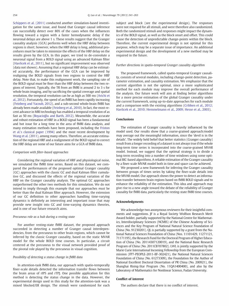
The classic Granger causality based on the whole time series failedto detect any significant3causal connectivity from the precuneus,while the AGC-OTWDA identified directional neural circuits centeredat the precuneus, as shown in Fig. 9. Since this dataset was collectedwhen the subjects' eyes were open, the information flows from theprecuneus and visual recognition network of the brain regions,marked in green in Fig. 9, were very significant.

To ascertain that the relative variation of the HRF is not a significantconfounding factor for the results of the precuneus, the cross-correlationfunction between the BOLD signals of two regions in each causal connec-tionwasexamined. The peaksof the cross-correlation function appearedto have zero lag in more than 90% of the subjects for most of the pairs,except for those between the right precuneus (PCUN.R), the rightPrecental gyrus (preCG.R), and the opercular part of the right inferiorfrontal gyrus (IFGoperc.R), which had only 68% peaks with zero lag.Therefore, the relative variation of the HRF was not a significant factorin the causality results between the precuneus and the visual recogni-tion network.

3 A significant causality was identified when its p-value was less than 0.05 in at least73% of the subjects.

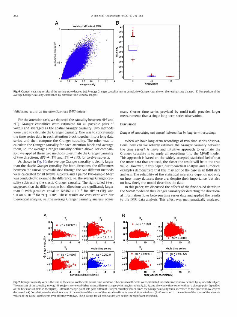
Fig. 6. Granger causality results of the resting-state dataset. (A) Average Granger causality versus cumulative Granger causality on the resting-state dataset. (B) Comparison of theaverage Granger causality established by different time window lengths.

252 Q. Luo et al. / NeuroImage 79 (2013) 241–263

Validating results on the attention-task fMRI dataset

For the attention task, we detected the causality between rIPS andrTPJ. Granger causalities were estimated for all possible pairs ofvoxels and averaged as the spatial Granger causality. Two methodswere used to calculate the Granger causality. One was to concatenatethe time series data in each attention block together into a long dataseries, and then compute the Granger causality. The other was tocalculate the Granger causality for each attention block and averagethem, i.e., the average Granger causality defined above. For compari-son, we applied these two methods to estimate the Granger causalityof two directions, rIPS ➔ rTPJ and rTPJ ➔ rIPS, for twelve subjects.

As shown in Fig. 10, the average Granger causality is clearly largerthan the classic Granger causality. For both directions, the differencesbetween the causalities established through the two different methodswere calculated for all twelve subjects, and a paired two-sample t-testwas conducted to examine the difference, i.e., the average Granger cau-sality subtracting the classic Granger causality. The right-tailed t-testsuggested that the differences in both directions are significantly largerthan 0 with p-values equal to 6.6482 × 10−6 for rIPS ➔ rTPJ, and9.0040 × 10−5 for rTPJ ➔ rIPS. These results are consistent with ourtheoretical analysis, i.e., the average Granger causality analysis across

Fig. 7. Granger causality versus the sum of the causal coefficients across time windows. TheThe medians of the causality among 198 subjects were established using different change-poas the titles for subplots in the figure). Different change-point sets gave different Granger cadecreased. (A) Correlation to the absolute value of the median of the sums of the causal coeffivalues of the causal coefficients over all time windows. The p-values for all correlations are

many shorter time series provided by multi-trails provides largermeasurements than a single long-term series observation.

Discussion

Danger of smoothing out causal information in long-term recordings

When we have long-term recordings of two time series observa-tions, how can we reliably estimate the Granger causality betweenthe time series? A naive and intuitive approach to estimate theGranger causality is to apply all recordings into the MVAR model.This approach is based on the widely-accepted statistical belief thatthe more data that are used, the closer the result will be to the truevalue. However, in this paper, our theoretical analysis and numericalexamples demonstrate that this may not be the case in an fMRI dataanalysis. The reliability of the statistical inference depends not onlyon how many datasets there are, despite their importance, but alsoon how finely the model describes the data.

In this paper, we discussed the effects of the fine-scaled details inthe MVAR model on the Granger causality for detecting the direction-al information flows between time series data and applied the resultsto the fMRI data analysis. This effect was mathematically analyzed,

causal coefficients were estimated for each time window defined by S1 for each subject.int sets, including S1, S2, S3, and the whole time series without a change-point (specifiedusality values, since the Granger causality value increased as the time window lengthscients over all time windows. (B) Correlation to the median of the sums of the absolutebelow the significant threshold.

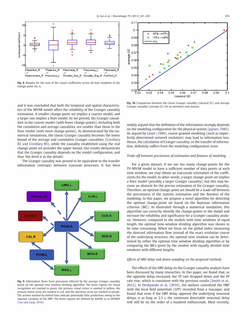
Fig. 10. Comparison between the classic Granger causality (classical GC) and averageGranger causality (average GC) for an attention-task dataset.

Fig. 8. Boxplot for the sum of the causal coefficients across all time windows of thechange-point set, S1.

253Q. Luo et al. / NeuroImage 79 (2013) 241–263

and it was concluded that both the temporal and spatial characteris-tics of the MVAR model affect the reliability of the Granger causalityestimation. A smaller change-point set implies a coarser model, anda larger one implies a finer model. As we proved, the Granger causal-ities in the coarser model (with fewer change-points), including boththe cumulative and average causalities, are smaller than those in thefiner model (with more change-points). As demonstrated by the nu-merical simulations, the classic Granger causality becomes the lowerbound of the average and cumulative Granger causalities (CorollaryB2 and Corollary B5), while the causality established using the realchange-point set provides the upper bound. Our results demonstratethat the Granger causality depends on the model configuration, andthus ‘the devil is in the details’.

The Granger causality was proved to be equivalent to the transferinformation (entropy) between Gaussian processes. It has been

Fig. 9. Information flows from precuneus inferred by the average Granger causalitybased on the optimal time window dividing algorithm. The brain regions for visualrecognition are marked in green, the primary visual cortex is marked in yellow, thesensory motor areas are marked in red, and the attention areas are marked in purple.The arrows marked by dotted lines indicate potentially false predictions owing to theregional variation of the HRF. The brain regions are defined by AAL90, as in DPARSF(Yan and Zang, 2010).

widely argued that the definition of the information strongly dependson the modeling configuration for the physical system (Jaynes, 1985).As argued by Lloyd (1989), coarse-grained modeling (such as imper-fectly determined network evolution) may lead to information loss.Hence, the calculation of Granger causality, or the transfer of informa-tion, definitely suffers from the modeling configuration issue.

Trade-off between preciseness of estimation and fineness of modeling

For a given dataset, if we use too many change-points for theTV-MVAR model to have a sufficient number of data points at eachtime window, we may obtain an inaccurate estimation of the coeffi-cients for the model. In other words, a larger change-point set impliesa finer model (possibly a larger Granger causality), but this may be-come an obstacle for the precise estimation of the Granger causality.Therefore, an optimal change-point set should be a trade-off betweenthe preciseness of the statistic estimation and the fineness of themodeling. In this paper, we propose a novel algorithm for detectingthe optimal change-point set based on the Bayesian informationcriterion (BIC). As illustrated through a numerical simulation, thisalgorithm can correctly identify the change-points in the model andincrease the reliability and significance for a Granger causality analy-sis. However, compared to the models with time windows of equallength, the optimal time-window dividing algorithm was shown tobe time consuming. When we focus on the global index measuringthe directed information flow instead of the exact evolution courseof the underlying structure, the optimal time window can be deter-mined by either the optimal time window dividing algorithm or bycomparing the BICs given by the models with equally divided timewindows with different lengths.

Effects of HRF delay and down-sampling on the proposed methods

The effects of the HRF delay on the Granger causality analysis havebeen discussed by many researches. In this paper, we found that, asthe opposite delay increased, the TP rate dropped down and the FPrate rose, which is consistent with the previous results (Smith et al.,2012). In Deshpande et al. (2010), the authors convolved the HRFwith the local field potentials (LFP) recorded from a macaque, andfound that even if the HRF delay opposed the underlying neuronaldelays is as long as 2.5 s, the minimum detectable neuronal delaywill still be on the order of a hundred milliseconds. Most recently,

254 Q. Luo et al. / NeuroImage 79 (2013) 241–263

Schippers et al. (2011) conducted another simulation-based investi-gation for the same issue, and found that Granger causal inferencecan successfully detect over 80% of the cases when the influencesflowing toward a region with a faster hemodynamic delay if theneuronal delays are above 1 s. These results suggest that the Grangercausality analysis (GCA) performs well when the HRF delay betweenregions is short; however, when the HRF delay is long, additional pro-cedures must be taken to minimize the effects of the HRF delay on theresults given by the GCA. In this paper, we tried to de-convolute aneuronal signal from a BOLD signal using an advanced Kalman filter(Havlicek et al., 2011), but no significant improvement was observed(data not shown). Assuming that a regional HRF delay can be estimat-ed accurately, the performance of the GCA can be improved byrealigning the BOLD signals from two regions to control the HRFdelay. Note that, to make this realignment work, the sampling rate ofthe BOLD signal must be finer than the HRF delay between the two re-gions of interest. Typically, the TR from an fMRI is around 2 to 3 s forwhole brain imaging, and by sacrificing the spatial coverage and spatialresolution, the temporal resolution can be as high as 500 ms (Arichi etal., 2012). Fortunately, the speed of an fMRI has been rapidly increasing(Feinberg and Yacoub, 2012), and a sub-second whole-brain fMRI hasalready beenmade available (Feinberg et al., 2010). In fact, the most re-cent advance inMRI technology has enabled a temporal resolution of asfast as 50 ms (Boyacioğlu and Barth, 2012). Meanwhile, the accurateand robust estimation of HRF in a BOLD signal has been a fundamentaland hot issue for a long time in the area of fMRI data analysis, andmany estimation methods have been proposed, including the Fristonet al.'s classical paper (1994) and the most recent development byWang et al. (2011), amongmany others. Therefore, an accurate estima-tion of the regional HRF and a realignment of the BOLD signal to correctthe HRF delay are some of our future aims for a GCA of fMRI data.

Comparison with filter-based approaches

Considering the regional variation of HRF and physiological noise,we simulated the fMRI time series. Based on this dataset, we com-pared the performances of the proposed optimal Granger causality(GC) approaches with the classic GC and dual Kalman filter cumula-tive GC, and discussed the effects of the regional variation of theHRF on the Granger causality analysis. The optimal GC approachesoutperformed the other two methods for this simulation. We do notintend to imply through this example that our approaches must bebetter than the dual Kalman filter approach. However, the extensionof our GC definition to other approaches handling time-varyingdynamics is definitely an interesting and important issue that mayprovide new insight into GC and time-varying dynamics theories,and is one of our future research aims.

Precuneus role as a hub during a resting state

For another resting-state fMRI dataset, the proposed approachsucceeded in detecting a number of Granger causal interdepen-dencies, from the precuneus to other brain regions, which cannot beinferred by the classic Granger causality, based on the static MVARmodel for the whole BOLD time courses. In particular, a circuitcentered at the precuneus to the visual network provided proof ofthe pivotal role played by the precuneus in visual cognition.

Possibility of detecting a status change in fMRI data

In attention-task fMRI data, our approach with spatio-temporallyfiner-scale details detected the information transfer flows betweenthe brain areas of rIPS and rTPJ. One possible application for thismethod is detecting the status change in the data. However, theexperimental design used in this study for the attention-task was amixed blocked/ER design. The stimuli were randomized for each

subject and block (see the experimental design). The responseswere not required for all stimuli, and were therefore also randomized.Both the randomized stimuli and responses might impact the dynam-ics of the BOLD signal, as well as the block onset and offset. This couldcause the detection of unpredictable change-points within the block.Therefore, the current experimental design is not optimal for thispurpose, which may be a separate issue of importance. An additionalexperimental design and the development of a new method may berequired in the future.

Further directions in spatio-temporal Granger causality algorithm

The proposed framework, called spatio-temporal Granger causali-ty, consists of several modules, including change-point detection, pa-rameter estimation, and causality estimation. We emphasize that thecurrent algorithm is not the optimal, since a more sophisticatedmethod for each module may improve the overall performance ofthe analysis. Our future work will aim at finding better algorithmsfor a more precise estimation of the global Granger causality underthe current framework, using up-to-date approaches for each moduleand a comparison with the existing algorithms (Cribben et al., 2012;Havlicek et al., 2010; Hemmelmann et al., 2009; Hesse et al., 2003).

Conclusions

The estimation of Granger causality is heavily influenced by themodel used. Our results show that a coarse-grained approach/modelmay average out the meaningful information, since the ‘devil is in thedetails’. The widely held belief that better statistics (Granger causality)result froma longer recording of a dataset is not always true if thewholelong-term time series is incorporated into the coarse-grained MVARmodel. Instead, we suggest that the optimal strategy is to divide along-term recording into a number of time windows using some opti-mal BIC-based algorithms. A reliable estimation of the Granger causalityby a finer-scale MVAR model both in time and space can be achieved.

We proposed a new framework for inferring the Granger causalitybetween groups of times series by taking the finer-scale details intotheMVARmodel. Our approach shows the power to detect an informa-tion transfer between brain regions based on fMRI BOLD signals and toenhance the reliability of the estimation. This idea and approach maygive rise to a new angle toward the debate of the reliability of Grangercausality for fMRI data, particularly the resting-state fMRI time courses.

Acknowledgments

We acknowledge two anonymous reviewers for their insightful com-ments and suggestions. JF is a Royal Society Wolfson Research MeritAward holder, partially supported by the National Centre for Mathemat-ics, Interdisciplinary Sciences (NCMIS) of the Chinese Academy of Sci-ences and the Key Program of National Natural Science Foundation ofChina (No. 91230201). QL is partially supported by a grant from the Na-tional Natural Sciences Foundation of China (Nos. 11101429, 11271121,71171195), the Research Fund for theDoctoral ProgramofHigher Educa-tion of China (No. 20114307120019), and the National Basic ResearchProgram of China (No. 2011CB707802). LWL is jointly supported by theMarie Curie International Incoming Fellowship from the European Com-mission (FP7-PEOPLE-2011-IIF-302421), the National Natural SciencesFoundation of China (No. 61273309), the Foundation for the Author ofNational Excellent Doctoral Dissertation of PR China (No. 200921), theShanghai Rising-Star Program (No. 11QA1400400), and also by theLaboratory of Mathematics for Nonlinear Science, Fudan University.

Conflict of interest

The authors declare that there is no conflict of interest.

255age 79 (2013) 241–263

Q. Luo et al. / NeuroIm

Appendix A. Solution of the time-varying linear regression

To build up a theoretical analysis of the Granger causality, we assume that the time series are generated by the following first-order(discrete-time) time-varying multivariate autoregressive (TV-MVAR) model:

x tþ1ð Þ ¼ a1 tð Þxt þ b1 tð Þyt þ n tð Þ; t ¼ 1;2; ⋯; T; ðA1Þ

where nt is white Gaussian noise statistically independent of x and y:

En tð Þ ¼ 0; E n tð Þn t′� �h i

¼ σ2n tð Þδt;t′ :

Here, δt,t ' is the Kronecker delta. Without loss of generality, we can suppose that xt and ytare centered, i.e., all means are equal to zeros, and thevariances of xt and yt both equal to 1, by multiplying coefficients a1(t) and b1(t) by their variances, respectively. Moreover, we assume that the cor-relation between xt and yt are stationary, i.e., E(xtyt) = c for a constant c ∈ [0,1]. Thus, we can perform a simple linear transformation tomake x andy orthogonal:

zt ¼yt−cxt� �ffiffiffiffiffiffiffiffiffiffiffiffi1−c2

p ;

which implies that zt has its mean equal to 0 and its variance equal to 1, and is uncorrelated with xt. Thus, (A1) becomes:

xtþ1 ¼ ~a1 tð Þxt þ ~b1 tð Þzt þ nt

with ~a1 tð Þ ¼ a1 tð Þ þ b1 tð Þc; ~b1 tð Þ ¼ b1 tð Þffiffiffiffiffiffiffiffiffiffiffiffi1−c2

p. Hence, we can discuss this problem assuming that xt and yt are uncorrelated that will not lose

generality. Therefore, in the following, we assume that xt and yt are uncorrelated.Considering the time-varying linear regression system (A1), we estimate the Granger causality with a different time-window split. More gen-

erally, we consider Eq. (2) or (3) to replace the intrinsic system. To estimate the theoretical values of the time-varying Granger causalities byaveraging or cumulating as mentioned in the main text, first, we are to estimate the parameters aS1

1 kð Þ and bS1ð Þ1 kð Þ by minimizing the following

residual square errors across the whole time interval:

∑T

t¼1E xtþ1−a

S11 kð Þxt−bS1

1 kð Þyt� �2 �

¼ ∑T

t¼1E a1 tð Þ−aS1

1 kð Þ� �

xt þ b1 tð Þ−bS11 kð Þ

� �xt þ nt

h i2� �¼ ∑

m

k¼1∑tk−1

t¼tk−1

E

("a1 tð Þ−aS1

1 kð Þ� �

xt

þ b1 tð Þ−bS11 kð Þ

� �yt þ nt �2g ¼ ∑

m

k¼1∑tk−1

t¼tk−1

a1 tð Þ−aS11 kð Þ

� �2 þ b1 tð Þ−bS11 kð Þ

� �2 þ σ2n tð Þ

�

which is equivalent to a series of minimization problems:

mina1S1 kð Þ ∑

tk−1

t¼tk−1

a1 tð Þ−aS11 kð Þ

� �2; mina1

S1 kð Þ ∑tk−1

t¼tk−1

b1 tð Þ−bS11 kð Þ

� �2for all k = 1, ⋯, m. It can be seen that the (expectation of) the solution should be

aS11 kð Þ ¼ 1

tk−tk−1∑tk−1

t¼tk−1

a1 tð Þ; bS11 kð Þ ¼ 1

tk−tk−1∑tk−1

t¼tk−1

b1 tð Þ; for allk: ðA2Þ

Appendix B. Monotonicity of the Ganger causalities of TV-MVAR models

Monotonicity of cumulative Granger causality

By the estimation of the coefficients, Eq. (A2), the cumulative Granger causality with the given time window lengths can be estimated as:

F c;S1ð ÞY→X ¼ log

US1þ∑T

t¼1 b1 tð Þð Þ2 þ∑Tt¼1σ

2n tð Þ

US1þ VS1

þ∑Tt¼1σ

2n tð Þ

!;

where

US1¼ ∑

m

k¼1∑tk−1

t¼tk−1

a1 tð Þ−aS11 kð Þ

� �2; VS1

¼ ∑m

k¼1∑tk−1

t¼tk−1

b1 tð Þ−bS11 kð Þ

� �2:

We have the following result.

256 Q. Luo et al. / NeuroImage 79 (2013) 241–263

Theorem B1. For two change-point sets S1 and S2, if S1 S2, then

F c;S1ð ÞY→X≤F c;S2ð Þ

Y→X :

Proof. Let S1 be composed of the following integer series:

1 ¼ t0bt1b⋯btm−1btm ¼ T þ 1:

Since the increasing integer series S2 contains S1, we can denote S2 as follows;

1 ¼ t0 ¼ð Þt11bt21b⋯btn11 btn1þ11 ¼ t12 ¼ t1ð Þ b⋯btnm−1þ1

m−1 ¼ t1m ¼ tm−1ð Þbt2mb⋯btnmm ¼ tmð Þ ¼ T þ 1:

In other words, in each time interval defined by S1, for instance, from tk − 1 to tk, we denote t1kbt2kb⋯bt

nkk btnkþ1

k as the integers in S2, which arelocated between tk − 1 and tk For simplicity, we let tnkþ1

k ¼ t1kþ1. Then, the TV-MVAR model with respect to S2 can be formulated as

xtþ1 ¼ aS21 k; qð Þxt þ bS2

1 k; qð Þxt þ ~n tð Þ; tqk≤tbtqþ1k ; q ¼ 1; ⋯;nk; k ¼ 1; ⋯;m: ðB1Þ

First, we are to prove that US1≥US2 and VS1≥VS2 are essentially the same. So, we need to prove one of them, for instance, VS1≥VS2 .In fact, we rewrite VS2 as follows:

VS2¼ ∑

S1j j

k¼1∑nk

q¼1∑

tqþ1k

−1

t¼tqk

b1 tð Þ−bS21 τ tqk

� � � �2where τ(tkq) denotes the order of tkq in the ordered integer set S2.

Thus, it is sufficient to show that in each time window of S1, it holds that

∑tk−1

t¼tk−1

b1 tð Þ−bS11 kð Þ

� �2≥∑nk

q¼1∑

tqþ1k

−1

t¼tqk

b1 tð Þ−bS21 τ tqk

� � � �2:

We note that

∑tk−1

t¼tk−1

b1 tð Þ−bS11 kð Þ

� �2 ¼ ∑tk−1

t¼tk−1

b1 tð Þ½ �2− tk−tk−1ð Þ bS11 kð Þ

h i2;∑

nk

q¼1∑

tqþ1k −1

t¼tqk

b1 tð Þ−bS21 τ tqk

� � � �2 ¼ ∑tk−1

t¼tk−1

b21 tð Þ−∑nk

q¼1tqþ1k −tqk

� �bS21 τ tqk

� � � �2and

bS11 kð Þ ¼ 1

tk−tk−1∑nk

q¼1tqþ1k −tqk

� �bS21 τ tqk

� � ;∑

nk

q¼1tqþ1k −tqk

� �¼ tk−tk−1:

Hence,

tk−tk−1ð Þ bS11 kð Þ

h i2 ¼ tk−tk−1ð Þ 1tk−tk−1

∑nk

q¼1tqþ1k −tqk

� �bS2

1

τ tqk� � " #2

≤ tk−tk−1ð Þ 1tk−tk−1

∑nk

q¼1tqþ1k −tqk

� �bS21 τ tqk

� � h i2 ¼ ∑nk

q¼1tqþ1k −tqk

� �bS21 τ tqk

� � h i2ðB2Þ

owing to the well-known fact that the weighted algebraic average is less than the square average with the weighting. This implies VS1≥VS2

. So, itis with US1

≥US2.

From VS1≥VS2 , we immediately have

∑Tt¼1 b1 tð Þð Þ2 þ∑T

t¼1σ2n tð Þ

VS1þ∑T

t¼1σ2n tð Þ ≤∑T

t¼1 b1 tð Þð Þ2 þ∑Tt¼1σ

2n tð Þ

VS2þ∑T

t¼1σ2n tð Þ :

Combined by US1≥US2 , we can derive

US1þ∑T

t¼1 b1 tð Þð Þ2 þ∑Tt¼1σ

2n tð Þ

US1þ VS1

þ∑Tt¼1σ

2n tð Þ ≤

US2þ∑T

t¼1 b1 tð Þð Þ2 þ∑Tt¼1σ

2n tð Þ

US2þ VS2

þ∑Tt¼1σ

2n tð Þ :

This means F c;S1ð ÞY→X≤F c;S2ð Þ

Y→X . From Eq. (B2), one can see that the inequality holds if and only if

bS21 τ tqk

� � ¼ bS11 kð Þ ðB3Þ

holds for all q = 1, ⋯, nk and all k.

257Q. Luo et al. / NeuroImage 79 (2013) 241–263

From Theorem B1 and its proof, in particular Eq. (B3) as the sufficient and necessary condition for F c;S1ð ÞY→X ¼ F c;S2ð Þ

Y→X . We immediately have theupper and lower bounds of the cumulative Granger causality.

Corollary B2. Let S0 = {1, T + 1} and S* be the ordered time point set that exactly comprise of the change-points in the TV-MVAR. Then, for anyordered time point set S, we have

F c;S0ð ÞY→X≤F c;Sð Þ

Y→X≤F c;S�ð ÞY→X :

This corollary shows that the static (classic) Granger causality actually is the lower-bound of the cumulative Granger causality. And, if thetime series are exactly generated by TV-MVAR (Eq. (A1)) with the change-point set S*, the cumulative Granger causality based on it is theupper bounds of all.

We should point out that Theorem B1 holds under the condition that one switching time set is contained in the other. It does not imply thatthe more change-points are, the larger cumulative Granger causality it will have.

Conjecture 1. If |S2| ≥ |S1|, then F c;S1ð ÞY→X≤F c;S2ð Þ

Y→X .We claim that this conjecture is not true by a simple counter example. Let T = 6, S1 = {1,4,7}, S2 = {1,3,5,7}, and S = {1,7}. We suppose that

the data is produced by the model (5) with a constant a1 and b1(t) is periodic with a period 2, i.e, b1(1) = b1(3) = b1(5) and b1(2) = b1(4) =b1(6). But the two values do not equal pair-wisely. It is clear that for S2, the parameters can be estimated as

bS21 1ð Þ ¼ bS2

1 2ð Þ ¼ bS21 3ð Þ ¼ 1

2b1 1ð Þ þ b1 2ð Þð Þ;

which equals to the whole average

b1 ¼ 16

b1 1ð Þ þ b1 2ð Þ þ b1 3ð Þ þ b1 4ð Þ þ b1 5ð Þ þ b1 6ð Þð Þ:

So, the corresponding Granger causality with S2 can be estimated equal to that of the static MVARmodel (the change-point is composed of S),i.e., F c;S2ð Þ

Y→X ¼ F c;Sð ÞY→X .

Noting thatF c;Sð ÞY→XbF

c;S1ð ÞY→X , where the strict inequality is because of b

S11 1ð Þ ¼ 1

3 b1 1ð Þ þ b1 2ð Þ þ b3 2ð Þð Þ≠b1. So,we haveF c;S2ð ÞY→X bF

c;S1ð ÞY→X despite |S2| > |S1|.

Let us consider a numerical example with a1(t) = 1, σn1(t) = 1 for all t, and b1(1) = b1(3) = b1(5) = 1 and b1(2) = b1(4) = b1(6) = 0. Direct

calculations lead that

F c;S1ð ÞY→X ¼ log

∑6t¼1 b1 tð Þð Þ2 þ 6

∑2k¼1∑3k

t¼3 k−1ð Þþ1 b1 tð Þ−bi1 kð Þ

� �2 þ 6

0B@1CA ¼ log

6þ 38=9þ 6

¼ log8162

:

However,

F c;S2ð ÞY→X ¼ log

∑6t¼1 b1 tð Þð Þ2 þ 6

∑3k¼1∑2k

t¼2 k−1ð Þþ1 b1 tð Þ−bi1 kð Þ

� �2 þ 6

0B@1CA ¼ log

6þ 33=2þ 6

¼ log65b log

8162

¼ F c;S1ð ÞY→X :

Monotonicity of average Granger causality

Another approach to estimate the Granger causality of TV-MVAR model is to estimate the Granger causality at each time windows (betweenswitching) can average them according to the length of each time window. Recall S1 = {1 = t0 b t1 b ⋯ b tm − 1 b tm = T + 1} as an increasinginteger sequence that denotes the change-point and the TV-MVAR model as

xtþ1 ¼ aS11 kð Þxt þ bS1

1 kð Þxt þ⌣n tð Þ; tk−1≤tbtk; k ¼ 1; ⋯;m: ðB4Þ

At each time window, the Granger causality can be estimated as

F k;S1ð ÞY→X ¼ log

Uk þ∑tk−1t¼tk−1

b1 tð Þð Þ2 þ∑tk−1t¼tk−1

σ2n tð Þ

Uk þ Vk þ∑tk−1t¼tk−1

σ2n tð Þ

!:

With

Uk ¼ ∑tk−1

t¼tk−1

a1 tð Þ−aS11 kð Þ

� �2;Vk ¼ ∑

tk−1

t¼tk−1

b1 tð Þ−bS11 kð Þ

� �2:

Then, we estimate the Granger causality by the TV-MVAR model (B4) as follows:

F a;S1ð ÞY→X ¼ 1

T∑m

k¼1F k;S1ð ÞY→X tk−tk−1ð Þ;

258 Q. Luo et al. / NeuroImage 79 (2013) 241–263

named the average Granger causality, the weighted average according to the lengths of the time windows. To investigate the relationshipbetween the average Granger causality and the fineness of temporal resolution, we need the following Lemma:

Lemma B3. For any positive integer T, any m real constants [ct]t = 1T , any T nonnegative constants [pt]t = 1

T with ∑Tt¼1pt ¼ 1 and any positive

constants [σt2]t = 1

T , we have the following inequality

log∑T

t¼1c2t pt þ σ2

∑tt¼1 ct−cð Þ2pt þ σ2

!≤∑

t

t¼1pt log

c2t þ σ2t

σ2t

!

where c ¼ ∑Tt¼1ptct and σ2 ¼ ∑T

t¼1ptσ2t .

Proof. Let us consider the following function with respect to C = [ct]t = 1T and Σ = [σt

2]t = 1T

V ¼ logσ2 þ c2

σ2 þ v−∑

T

t¼1pt log

σ2t þ c2tσ2

t

!

with

c2 ¼ ∑T

t¼1c2t pt ; v ¼ ∑

T

t¼1c tð Þ−c½ �2pt ¼ c2− cð Þ2:

We make minor modifications on the problem according to the following three facts. First, noting

v ¼ ∑T

t¼1ct−c½ �2pt ¼ ∑

T

t¼1ct½ Þ�2pt− ∑

T

t¼1ctpt

!2

≥∑T

t¼1jct 2pt− ∑

T

t¼1ctj jpt

!2

;

if we replace ct by |ct| in V, which is denoted by V , then we have V≤V .

Therefore, without loss of generality, it is sufficient to prove V≤0 by considering the case that all ct are nonnegative.Second, considering

∂V∂ctjct¼0 ¼ 2cptσ2 þ v;

which is positive in the case that there is at least one positive ct with nonzero pt. So, it is sufficient to consider the case that all ct are positive;Third, it holds

∑T

t¼1pt log σ2

t

� �≤ log σ2

� �owing to the Jensen's inequality.

In summary, we can consider the following function instead of V:

~V y; v;Σð Þ ¼ logσ2 þ c2

σ2 þ v−∑

T

t¼1pt log

σ2t þ ytσ2

!:

Letting yt = (ct)2, owing to the fact that all ct are nonnegative, y = [yt], with fixed c2 and σ2, we are going to show that ~V is nonnegative byconsidering the following maximization problem:

max~V y; v;Σð Þs:t:XTt¼1

ytpt ¼ c2;∑T

t¼1

ffiffiffiffiffiyt

ppt ¼

ffiffiffiffiffiffiffiffiffiffiffiffic2−v

p;∑

T

t¼1ptσ

2t ¼ σ2

;σ2t > 0; yt > 0;∀t: ðB5Þ

To solve Eq. (B5), we introduce the following auxiliary Lagrange function:

L y; v;Σ;λ; μ;γð Þ¼ ~V

y; v;Σð Þ þ λ ∑T

t¼1ytpt−b2

!þ μ ∑

T

t¼1

ffiffiffiffiffiyt

ppt−

ffiffiffiffiffiffiffiffiffiffiffiffic2−v

p !þ γ ∑

T

t¼1σ2

t pt−σ2

!:

By the Karush–Kuhn–Tucker conditions, the necessary conditions of the minimum of Eq. (B5) include:

∂L∂yt

¼ pt − 1σ2

t þ yt� þ λþ μ

2ffiffiffiffiffiyt

p" #

¼ 0;

∂L∂v ¼ − 1

σ2 þ vþ μ

2ffiffiffiffiffiffiffiffiffiffiffiffic2−v

p ¼ 0;

259Q. Luo et al. / NeuroImage 79 (2013) 241–263

∂L∂ σ2

t

� ¼ pt − 1σ2

t þ yt� þ γ

" #¼ 0:

This leads (i) pt = 0 or (ii) σt2 + yt = 1/γ and

yt ¼μ

2 γ−λð Þ �2

: ðB6Þ

In other words, for these yt with nonzero pt, if we are to solve yt from the above equalities as a function with respect to σ, λ, μ, γ, c2 and v,which are independent of the index t, then we can only have one expression from Eq. (B6). It should be emphasized that we are not solving thevalues of yt but its expression with respect to the t-independent quantities, σ, λ, μ, γ, c2 and v. Therefore, the possible minimum points of R(y,v)only has one single value of yt. So it is with

σ2t ¼ 1

γ− μ

2 γ−λð Þ �2

:

It can be seen that if yt and σt2 can only have a single value respectively, then ~V y; v;Σð Þ ¼ 0. So, the maximum of ~V y; v;Σð Þ is zero. Hence, the

intrinsic V has its maximum equal to zero. Therefore, Lemma B3 is proved and the equality holds if and only if yt and σt2 can only have a single

value respectively.Theorem B4. Let S1 and S2 be two sequences of increasing integers. If S1 S2, then

F a;S1ð ÞY→X≤F a;S2ð Þ

Y→X :

Proof. We denote the sets S1 and S2 by the symbols as in the proof of Theorem B1. According to Eq. (B1), the Granger causality at the timewindow of S2, the k-th window of S1 and the q-th can be written as:

F k;q;S2ð ÞY→X ¼ log

Uk;q þ∑tqþ1k

−1

t¼tqk

b1 tð Þð Þ2 þ∑tqþ1k

−1

t¼tqk

σ2n tð Þ

Uk;q þ Vk;q þ∑tqþ1k

−1

t¼tqk

σ2n tð Þ

0B@1CA

where

Uk;q ¼ ∑tqþ1k

−1

t¼tqk

a1 tð Þ−aS21 τ tqk

� � � �2;Vk;q ¼ ∑

tqþ1k

−1

t¼tqk

b1 tð Þ−bS21 τ tqk

� � � �2:

Then, the average Granger causality with respect to S2 is

F a;S2ð ÞY→X ¼ 1

T∑S1j j

k¼1∑nk

q¼1F k;q;S2ð ÞY→X tqþ1

k −tqk� �

:

Note

∑nk

q¼1aS21 τ tqk

� � tqþ1k −tqk

� �¼ aS1

1 kð Þ;∑nk

q¼1bS21 τ tqk

� � tqþ1k −tqk

� �¼ bS1

1 kð Þ;

and

∑tqþ1k

−1

t¼tqk

a1 tð Þ½ �2 ¼ ∑tqþ1k

−1

t¼tqk

a1 tð Þ−aS21 τ tqk

� � h i2 þ aS21 τ tqk

� � h i2tqþ1k −tqk

� �;

∑tqþ1k −1

t¼tqk

b1 tð Þ½ �2 ¼ ∑tqþ1k −1

t¼tqk

a1 tð Þ−bS21 τ tqk

� � h i2 þ bS21 τ tqk

� � h i2tqþ1k −tqk

� �:

Compared with F a;S2ð ÞY→X , we can rewrite the term of F a;S1ð Þ

Y→X , i.e., Fk;S1ð ÞY→X , as follows:

F k;S1ð ÞY→X ¼ log

Uk þ∑tk−1t¼tk−1

b1 tð Þð Þ2 þ∑tk−1t¼tk−1

σ2n tð Þ

Uk þ Vk þ∑tk−1t¼tk−1

σ2n tð Þ

!¼ log

�∑nk

q¼1aS11 kð Þ−aS2

1 τ tqk� � h i2

tqþ1k −tqk

� �þ∑

nk

q¼1bS21 τ tqk

� � h i2tqþ1k −tqk

� �

þ∑nk

q¼1ε2n qð Þ tqþ1

k −tqk� �

Þ−log ∑nk

q¼1aS11 kð Þ−aS2

1 τ tqk� � h i2

tqþ1k −tqk

� �þ∑

nk

q¼1bS11 kð Þ−bS2

1 τ tqk� � h i2

tqþ1k −tqk

� �þ∑

nk

q¼1ε2n qð Þ tqþ1

k −tqk� � !

260 Q. Luo et al. / NeuroImage 79 (2013) 241–263

where

ε2n qð Þ ¼ 1

tqþ1k −tqk

∑tqþ1k

−1

t¼tqk

a1 tð Þ−aS21 τ tqk

� � h i2 þ b1 tð Þ−bS21 τ tqk

� � h i2 þ σ2n tð Þ

� �:

Since

∑nkq¼1 aS1

1 kð Þ−aS21 τ tqk

� � h i2tqþ1k −tqk

� �þ∑nk

q¼1 bS21 τ tqk

� � h i2tqþ1k −tqk

� �þ∑nk

q¼1ε2n qð Þ tqþ1

k −tqk� �

∑nkq¼1 aS1

1 kð Þ−aS21 τ tqk

� � h i2tqþ1k −tqk

� �þ∑nk

q¼1 bS11 kð Þ−bS2

1 τ tqk� � h i2

tqþ1k −tqk

� �þ∑nk

q¼1ε2n qð Þ tqþ1

k −tqk� �

≤∑nk

q¼1 bS21 τ tqk

� � h i2tqþ1k −tqk

� �þ∑nk

q¼1ε2n qð Þ tqþ1

k −tqk� �

∑nkq¼1 bS1

1 kð Þ−bS21 τ tqk

� � h i2tqþ1k −tqk

� �þ∑nk

q¼1ε2n qð Þ tqþ1

k −tqk� � :

Theorem B4 can be derived by directly employing Lemma B3. In addition, the inequality holds if and only if bS21 τ tqk

� � and εn2(q) can only pick

values independent of the index q (but possibly depending on the index k), respectively.Similar to Corollary B2, from Theorem B4 and its proof, in particular the sufficient and necessary condition for F a;S1ð Þ

Y→X ¼ F a;S2ð ÞY→X . We immediately

have the upper and lower bounds of the cumulative Granger causality.Corollary B5. Let S0 = {1, T + 1} and S* be the ordered time point set that exactly comprise of the change-points in the TV-MVAR model. Then, for

any ordered time point set S, we have

F a;S0ð ÞY→X≤F a;Sð Þ

Y→X≤F a;S�ð ÞY→X :

This corollary shows that the static (classic) Granger causality actually is the lower-bound of the average Granger causality. And, if the timeseries are exactly generated by TV-MVAR (Eq. (A1)) with the change-point set S*, the average Granger causality based on it is the upper boundsof all.

We should also emphasize that the following conjecture is not true.Conjecture B2. If |S2| ≥ |S1|, then F a;S1ð Þ

Y→X≤F a;S2ð ÞY→X .

That is to say, the average Granger causality is monotonic with respect to the containing relation between the change-point set, but notmonotonic with respect to the size of the change-point sets. A counter-example can be easily established by the same way as in Conjecture 1.

Appendix C. Comparison between cumulative and average Ganger causalities

Magnitude comparison

Actually, the two sorts of Granger causalities of the TV-MVAR model do not have definite magnitude relation. First, we show in the followingtheorem, the relation that cumulative Granger causality is greater than the average Granger causality with the same change-point set isconditional.

Theorem C1. Let S be a sequence of increasing integers. If the following quantity

1tk−tk−1

∑tk−1

t¼tk−1

a1 tð Þ−a1 kð Þð Þ2 þ ∑tk−1

t¼tk−1

b1 tð Þ−b1 kð Þ� �2 þ ∑

tk−1

t¼tk−1

σ2n tð Þ

" #

with

a1 kð Þ ¼ 1tk−tk−1

∑tk−1

t¼tk−1

a1 tð Þ; b1 kð Þ ¼ 1tk−tk−1

∑tk−1

t¼tk−1

b1 tð Þ

is independent of the index k, then

F a;Sð ÞY→X≤F c;Sð Þ

Y→X :

Proof. Let S = {1 = t0 b t1 b ⋯ b tm − 1 b tm = T + 1}. And, with the same notations we used above, we have

F c;Sð ÞY→X ¼ log

∑mk¼1∑

tk−1t¼tk−1

a1 tð Þ−a1 kð Þð Þ2 þ∑Tt¼1 b1 tð Þð Þ2 þ∑T

t¼1σ2n tð Þ

∑mk¼1∑

tk−1t¼tk−1

a1 tð Þ−a1 kð Þð Þ2 þ∑mk¼1∑

tk−1t¼tk−1

b1 tð Þ−b1 kð Þ� �2 þ∑T

t¼1σ2n tð Þ

0B@1CA;

and

F a;Sð ÞY→X ¼ 1

T∑m

k¼1tk−tk−1ð Þ log ∑tk−1

t¼tk−1a1 tð Þ−a1 kð Þð Þ2 þ∑tk−1

t¼tk−1b1 tð Þð Þ2 þ∑tk−1

t¼tk−1σ2

n tð Þ∑tk−1

t¼tk−1a1 tð Þ−a1 kð Þð Þ2 þ∑tk−1

t¼tk−1b1 tð Þ−b1 kð Þ� �2 þ∑tk−1

t¼tk−1σ2

n tð Þ

0B@1CA:

261Q. Luo et al. / NeuroImage 79 (2013) 241–263

Let b1 ¼ 1T ∑

Tt¼1b1 tð Þ. Thus, we can rewrite them as

F c;Sð ÞY→X ¼ log

∑mk¼1∑

tk−1t¼tk−1

a1 tð Þ−a1 kð Þð Þ2 þ∑mt¼1 b1 kð Þ� �2

tk−tk−1ð Þ þ∑mt¼1∑

tk−1t¼tk−1

b1 tð Þ−b1 kð Þ� �2 þ∑T

t¼1σ2n tð Þ

∑mk¼1∑

tk−1t¼tk−1

a1 tð Þ−a1 kð Þð Þ2 þ∑mk¼1∑

tk−1t¼tk−1

b1 tð Þ−b1 kð Þ� �2 þ∑T

t¼1σ2n tð Þ

0B@1CA

and

F a;Sð ÞY→X ¼ 1

T∑m

k¼1tk−tk−1ð Þ � log

∑tk−1t¼tk−1

a1 tð Þ−a1 kð Þð Þ2 þ∑tk−1t¼tk−1

b1 tð Þ−b1 kð Þ� �2 þ b1 kð Þ

� �2tk−tk−1ð Þ þ∑tk−1

t¼tk−1σ2

n tð Þ

∑tk−1t¼tk−1

a1 tð Þ−a1 kð Þð Þ2 þ∑tk−1t¼tk−1

b1 tð Þ−b1 kð Þ� �2 þ∑tk−1

t¼tk−1σ2

n tð Þ

0B@1CA:

In addition, letting

θk ¼1

tk−tk−1∑tk−1

t¼tk−1

a1 tð Þ−a1 kð Þð Þ2 þ ∑tk−1

t¼tk−1

b1 tð Þ−b1 kð Þ� �2 þ ∑

tk−1

t¼tk−1

σ2n tð Þ

" #;αk ¼

1tk−tk−1

∑tk−1

t¼tk−1

b1 kð Þ� �2

;pk ¼tk−tk−1ð Þ

T

due to the condition, θk is independent of k, which is denoted by θ. Thus, we have

F c;Sð ÞY→X ¼ log

∑mt¼1αkpk þ∑m

k¼1θkpk∑m

k¼1θkpk

� �¼ log

∑mt¼1αkpk þ θ

θ

� �;

and

F a;Sð ÞY→X ¼ ∑

m

k¼1pk log

αk þ θkθk

� �¼ ∑

m

k¼1pk log

αk þ θθ

� �:

Thus, we can conclude FY → X(a,S) ≤ FY → X

(c,S) , owing to the Jensen's inequality. This completes the proof.From Theorem C1, if the TV-MVAR system is time-varying with the segments well known, which implies that at each time window, the sys-

tem is static, we can conclude that the average Grange causality is smaller than the cumulative Granger causality.On the other hand, if the condition in Theorem C1 is not satisfied, then it will not be surprising that FY → X

(a,S) > FY → X(c,S) holds. Here is a

counter-example. A special situation is to solve the time-varying regression model (A1) as a static one, i.e., taking all time points as thechange-point set, i.e., S = {1, ⋯, T + 1}. By a proper transformation, we can still let the variances of y and x equal to 1 for all time. Leta1(t) = 0 for all t. But the variance of the noise may be time-varying. The defined Granger causalities become:

FSY→X ¼ log1T ∑

Tt¼1σ

2n tð Þ þ 1

T ∑Tt¼1 b1 tð Þ½ �2

1T ∑

Tt¼1σ

2n tð Þ

!; F S

Y→X ¼ 1T∑T

t¼1log

σ2n tð Þ þ b1 tð Þ½ �2

σ2n tð Þ

!:

Pick T = 3, b1 = 1,b2 ¼ffiffiffi2

p; b3 ¼

ffiffiffi3

p;σ1 ¼

ffiffiffi3

p;σ2 ¼

ffiffiffi2

p;σ3 ¼ 1. Then,

FY→X ¼ log2bF Y→X ¼ 13

log43

� �þ log 2ð Þ þ log 4ð Þ

�:

Comparison between the asymptotic square moments under null hypothesis

For simplicity, we suppose that the time-varying system (A1) is a switching systemwith equal-length time windows and the segment pointsare exactly known. The general case will be treated in our future paper. Thus, (A1) becomes a series of static linear system as follows:

xtþ1 ¼ a1 kð Þxt þ b1 kð Þyt þ n tð Þ; tk≤tbtkþ1; k ¼ 1;2; ⋯m: ðC1Þ

Here, tkþ1−tk ¼ nm for all k. Under the null hypothesis, namely, the coefficients b1(t) = 0 hold for all t, Eq. (C1) becomes

xtþ1 ¼ a1 kð Þxt þ ~n tð Þ; tk≤tbtkþ1; k ¼ 1;2; ⋯m: ðC2Þ

Their residual squared errors at each time window are

RSS1 kð Þ ¼ ∑tkþ1−1

t¼tkn2 tð Þ and RSS0 kð Þ ¼ ∑

tkþ1−1

t¼tk

~n2 tð Þ:

Then, the CGS and AGC can be formulated as follows respectively:

FcY→X ¼ log∑m

k¼1RSS0 kð Þ∑m

k¼1RSS1 kð Þ� �

¼ log 1þ∑mk¼1 RSS0 kð Þ−RSS1 kð Þ½ �

∑mk¼1RSS1 kð Þ

� �e∑mk¼1 RSS0 kð Þ−RSS1 kð Þ½ �

∑mk¼1RSS1 kð Þ

262 Q. Luo et al. / NeuroImage 79 (2013) 241–263

FaY→X ¼ 1m

∑m

k¼1log

RSS0 kð ÞRSS1 kð Þ� �

¼ 1m

∑m

k¼1log 1þ RSS0 kð Þ−RSS kð Þ

RSS1 kð Þ� �e 1

m∑m

k¼1

RSS0 kð Þ−RSS1 kð ÞRSS1 kð Þ

as n goes to infinity. Therefore, the cumulative Granger causality converges the following in distribution:

FcY→X � n−2m−1m

≈∑mk¼1 RSS0 kð Þ−RSS1 kð Þ½ �

∑mk¼1RSS1 kð Þ � n−2m−1

meF m;n−2m−1ð Þ

and the average Granger causality converges to:

FaY→X � n=m−31

≈ 1m

∑m

k¼1

RSS0 kð Þ−RSS1 kð ÞRSS1 kð Þ � n=m−3

1

with each

RSS0 kð Þ−RSS1 kð ÞRSS1 kð Þ � n=m−3

1eF 1;

nm

−3� �

:

So, their asymptotic expectations are

E FcY→X

� ≈ m

n−2m−1n−2m−1n−2m−3

¼ 1nm−2− 3

m

; E FaY→X

� ≈

nm−3nm−5

1nm−3

¼ 1nm−5

;

as n → ∞.The dominant converge rates are the same, equivalently m

n : Then, let us take a look at their asymptotic square moments. By the square mo-ment of the F-distribution and simple algebras, we have

E FcY→X

� �2n o≈ 1þ 2

m

� �mn

� �2:

As for the AGC, with f k ¼ RSS0 kð Þ−RSS1 kð ÞRSS1 kð Þ eF 1; nm−3

� , we have

E FaY→X

� �2n o≅ 1

n=m−3

� �2E

1m

∑m

k¼1f k

� �2

≤ 1n=m−3

� �2 1m

� �∑m

k¼1E f kf g2

with

E f 2kn o

≅3nm−3nm−5

� �2

;

which implies

E FaY→X

� �2n ob3m

mn

� �2holds in the asymptotic sense, i.e, if n is a sufficiently large. Therefore, in the asymptotic squared meaning, for m > 1, we have

E FaY→X

� �2n obE FcY→X

� �2n oasymptotically. In other words, the average Granger causality converges to zero more quickly than the cumulative Granger causality.

Theorem C2. Under the setup as mentioned above, limsupn→∞E FaY→X½ �2� �

E FcY→X½ �2� �b1 for m > 1.

And, the larger m is, the higher asymptotic converge rate the average Granger causality is than the cumulative one.

Appendix D. Dual Kalman filter cumulative Granger causality (Dkf cumulative GC)

We used the dual Kalman filter as in Havlicek et al. (2010), Sommerlade et al. (2012), which can be described as the following MVAR

xtþ1

ytþ1

�¼Xpk¼1

Ak tð Þ xt�k

yt�k

�þ nt

1nt2

�ðD1Þ

where Ak(t) are the time-varying coefficients and n1,2t are the white noises. Define

zt ¼ xt

yt

�; w tð Þ ¼ zt

� �T; ⋯; ; zt−pþ1

� �Th iT; a tð Þ ¼ vec A1 tð ÞT ; ⋯;Ak tð ÞT

h i� �;

263Q. Luo et al. / NeuroImage 79 (2013) 241–263

and Eq. (D1) can be rewritten as

zt ¼ w t−1ð ÞTa tð Þ þ ηt ðD2Þ

associated with a random walk process for the time-varying coefficients

a t þ 1ð Þ ¼ a tð Þ þ νt: ðD3Þ

By the dual Kalman filter approach, the time-varying coefficients can be estimated, and then the residuals of Eq. (D2) can be used to define acumulative GC by the same fashion as the cumulative GC in the paper

dkfGCY→X ¼ log

XTt¼1

var ηtyx� �

XTt¼1

var ηtx� �

0BBBB@1CCCCA; ðD4Þ

where T is the length of the time course, ηyxt is the noise term in Eq. (D2) for the x-component with considering the inter-dependence from they-component, and ηxt is the noise term in Eq. (D2) without considering the inter-dependence from the y-component. As in Havlicek et al. (2010),the dkfGCY → X and the dkfGCX → Y can be computed by estimating the model parameters, and the p-value of these causality statistics can beestablished by a bootstrap. The readers are referred to Havlicek et al. (2010) for more details about the parameter estimation procedure andthe bootstrap for significance.

References

Ahmed, A., Xing, E., 2009. Recovering time-varying networks of dependencies in socialand biological studies. Proc. Natl. Acad. Sci. 106, 11878–11883.

Arichi, T., Fagiolo, G., Varela, M., Melendez-Calderon, A., Allievi, A., Merchant, N., Tusor, N.,Counsell, S.J., Burdet, E., Beckmann, C.F., Edwards, A.D., 2012. Development of BOLDsignal hemodynamic responses in the human brain. Neuroimage 63, 663–673.

Biswal, B., Mennes, M., Zuo, X.-N., et al., 2010. Toward discovery science of human brainfunction. Proc. Natl. Acad. Sci. 107, 4734–4739.

Boyacioğlu, R., Barth,M., 2012. Generalized iNverse imaging (GIN): Ultrafast fMRIwith phys-iological noise correction. Magn. Reson. Med. http://dx.doi.org/10.1002/mrm.24528.

Cavanna, A.E., Trimble, M.R., 2006. The precuneus: a review of its functional anatomyand behavioural correlates. Brain 129, 564–583 (Epub 2006 Jan 2006).

Chen, M.-P., Lee, C.-C., Hsu, Y.-C., 2011. The impact of American depositary receipts onthe Japanese index: do industry effect and size effect matter? Econ. Model. 28,526–539.

Cribben, I., Haraldsdottir, R., Atlas, L.Y., Wager, T.D., Lindquist, M.A., 2012. Dynamicconnectivity regression: determining state-related changes in brain connectivity.Neuroimage 61, 907–920.

Deshpande, G., Sathian, K., Hu, X., 2010. Effect of hemodynamic variability on Grangercausality analysis of fMRI. Neuroimage 52, 884–896.

Ding, M., Bressler, S.L., Yang, W., Liang, H., 2000. Short-window spectral analysis of corti-cal event-related potentials by adaptive multivariate autoregressive modeling: datapreprocessing, model validation, and variability assessment. Biol. Cybern. 83, 35–45.

Evan, K., Snigdhansu, C., Auroop, R.G., 2011. Exploring Granger causality between glob-al average observed time series of carbon dioxide and temperature. Theor. Appl.Climatol. 104, 325–335.

Feinberg, D.A., Yacoub, E., 2012. The rapid development of high speed, resolution andprecision in fMRI. Neuroimage 62, 720–725.

Feinberg, D.A., Moeller, S., Smith, S.M., Auerbach, E., Ramanna, S., Glasser, M.F., Miller, K.L.,Ugurbil, K., Yacoub, E., 2010. Multiplexed echo planar imaging for sub-second wholebrain FMRI and fast diffusion imaging. PLoS One 5, e15710.

Friston, K.J., Jezzard, P., Turner, R., 1994. Analysis of functional MRI time-series. Hum.Brain Mapp. 1, 153–171.

Friston, K., Moran, R., Seth, A.K., 2012. Analysing connectivity with Granger causalityand dynamic causal modelling. Curr. Opin. Neurobiol. 23, 1–7.

Ge, T., Kendrick, K., Feng, J., 2009. A novel extended granger causal model approachdemonstrates brain hemispheric differences during face recognition learning.PLoS Comput. Biol. 5, e1000570.

Ge, T., Feng, J., Grabenhorst, F., Rolls, E., 2012. Componential Granger causality, and itsapplication to identifying the source and mechanisms of the top-down biased ac-tivation that controls attention to affective vs sensory processing. Neuroimage59, 1846–1858.

Granger, C.W.J., 1969. Investigating causal relations by econometric models and cross-spectral methods. Econometrica 37, 424–438.

Guo, S., Wu, J., Ding, M., Feng, J., 2008. Uncovering Interactions in the frequency domain.PLoS Comput. Biol. 4, e1000087.

Havlicek, M., Jan, J., Brazdil, M., Calhoun, V.D., 2010. Dynamic Granger causality basedon Kalman filter for evaluation of functional network connectivity in fMRI data.Neuroimage 53, 65–77.

Havlicek, M., Friston, K.J., Jan, J., Brazdil, M., Calhoun, V.D., 2011. Dynamicmodeling of neu-ronal responses in fMRI using cubature Kalman filtering. Neuroimage 56, 2109–2128.

Hemmelmann, D., Ungureanu, M., Hesse, W., Wustenberg, T., Reichenbach, J.R., Witte,O.W., Witte, H., Leistritz, L., 2009. Modelling and analysis of time-variant directedinterrelations between brain regions based on BOLD-signals. Neuroimage 45,722–737.

Hesse, W., Moller, E., Arnold, M., Schack, B., 2003. The use of time-variant EEG Grangercausality for inspecting directed interdependencies of neural assemblies. J. Neurosci.Methods 124, 27–44.

Jaynes, E.T., 1985. Some random observations. Synthese 63, 115–138.Lloyd, S., 1989. Use of mutual information to decrease entropy: implications for the

second law of thermodynamics. Phys. Rev. A 39, 5378–5386.Luo, Q., Ge, T., Feng, J., 2011. Granger causality with signal-dependent noise. Neuroimage

57, 1422–1429.Luscombe, N.M., Madan Babu, M., Yu, H., Snyder, M., Teichmann, S.A., Gerstein, M.,

2004. Genomic analysis of regulatory network dynamics reveals large topologicalchanges. Nature 431, 308–312.

Ohiorhenuan, I.E., Mechler, F., Purpura, K.P., Schmid, A.M., Hu, Q., Victor, J.D., 2010.Sparse coding and high-order correlations in fine-scale cortical networks. Nature466, 617–621.

Psaradakis, Z., Ravn, M.O., Sola, M., 2005. Markov switching causality and the money–output relationship. J. Appl. Econ. 20, 665–683.

Sato, J.o.R., Junior, E.A., Takahashi, D.Y., de Maria Felix, M., Brammer, M.J., Morettin, P.A.,2006. A method to produce evolving functional connectivity maps during thecourse of an fMRI experiment using wavelet-based time-varying Granger causality.Neuroimage 31, 187–196.

Schippers, M., Renken, R., Keysers, C., 2011. The effect of intra- and inter-subject vari-ability of hemodynamic responses on group level Granger causality analyses.Neuroimage 57, 22–36.

Smerieri, A., Rolls, E.T., Feng, J., 2010. Decision time, slow inhibition, and theta rhythm.J. Neurosci. 30, 14173–14181.

Smith, S.M., Miller, K.L., Salimi-khorshidi, G., Webster, M., Beckmann, C.F., Nichols, T.E.,Ramsey, J.D.,Woolrich, M.W., 2011. Networkmodellingmethods for FMRI. Neuroimage54, 875–891.

Smith, S.M., Bandettini, P.A., Miller, K.L., Behrens, T.E., Friston, K.J., David, O., Liu, T.,Woolrich, M.W., Nichols, T.E., 2012. The danger of systematic bias in group-levelFMRI-lag-based causality estimation. Neuroimage 59, 1228–1229.

Sommerlade, L., Thiel, M., Platt, B., Plano, A., Riedel, G., Grebogi, C., Timmer, J., Schelter,B., 2012. Inference of Granger causal time-dependent influences in noisy multivar-iate time series. J. Neurosci. Methods 203, 173–185.

Tuncbag, N., Kar, G., Gursoy, A., Keskin, O., Nussinov, R., 2009. Towards inferring timedimensionality in protein–protein interaction networks by integrating structures:the p53 example. Mol. Biosyst. 5, 1770–1778.

Tzourio-Mazoyer, N., Landeau, B., Papathanassiou, D., Crivello, F., Etard, O., Delcroix, N.,Mazoyer, B., Joliot, M., 2002. Automated anatomical labeling of activations in SPMusing a macroscopic anatomical parcellation of the MNI MRI single-subject brain.Neuroimage 15, 273–289.

Wang, J., Zhu, H., Fan, J., Giovanello, K., Lin, W., 2011. Adaptively and spatially estimat-ing the hemodynamic response functions in fMRI. Med. Image Comput. Comput.Assist. Interv. 14, 269–276.

Wen, X., Yao, L., Liu, Y., Ding, M., 2012. Causal interactions in attention networkspredict behavioral performance. J. Neurosci. 32, 1284–1292.

Wiener, N., 1956. The theory of prediction. In: BeckenBach, E. (Ed.), Modern Mathe-matics for the Engineer. McGraw-Hill, New York, pp. 165–190.

Yan, C., Zang, Y., 2010. DPARSF: a MATLAB toolbox for “pipeline” data analysis ofresting-state fMRI. Front. Syst. Neurosci. 4.

Zalesky, A., Fornito, A., Harding, I.H., Cocchi, L., Yucel, M., Pantelis, C., Bullmore, E.T.,2010. Whole-brain anatomical networks: does the choice of nodes matter?Neuroimage 50, 970–983.

Zhu, J., Chen, Y., Leonardson, A.S., Wang, K., Lamb, J.R., Emilsson, V., Schadt, E.E., 2010.Characterizing dynamic changes in the human blood transcriptional network. PLoSComput. Biol. 6, e1000671.