Remote Sensing of Environment 113 (2009) 2606–2617

Contents lists available at ScienceDirect

Remote Sensing of Environment

j ourna l homepage: www.e lsev ie r.com/ locate / rse

Spatial–temporal dynamics of land surface temperature in relation to fractionalvegetation cover and land use/cover in the Tabriz urban area, Iran

Reza Amiri a, Qihao Weng b,⁎, Abbas Alimohammadi c, Seyed Kazem Alavipanah d

a School of Geography and Environmental Science, Monash University, Clayton, Victoria 3800, Australiab Center for Urban and Environmental Change, Department of Geography, Geology, and Anthropology, Indiana State University, Terre Haute, IN 47809, USAc Department of GIS, K. N. Toosi University of Technology, Tehran, Irand Department of Cartography, Faculty of Geography, University of Tehran, Tehran, Iran

⁎ Corresponding author. Tel.: +1 812 237 2255; fax:E-mail addresses: reza.amiri@arts.monash.edu.au (R

(Q. Weng), alimoh_abb@kntu.ac.ir (A. Alimohammadi),(S.K. Alavipanah).

0034-4257/$ – see front matter © 2009 Elsevier Inc. Aldoi:10.1016/j.rse.2009.07.021

a b s t r a c t

a r t i c l e i n f o

Article history:Received 6 October 2008Received in revised form 22 July 2009Accepted 23 July 2009

Keywords:Land surface temperatureVegetation coverTVX spaceLULC changeUrban

Rapid changes of land use and land cover (LULC) in urban areas have become a major environmental concerndue to environmental impacts, such as the reduction of green spaces and development of urban heat islands(UHI). Monitoring and management plans are required to solve this problem effectively. The Tabrizmetropolitan area in Iran, selected as a case study for this research, is an example of a fast growing city.Multi-temporal images acquired by Landsat 4, 5 TM and Landsat 7 ETM+ sensors on 30 June 1989, 18 August1998, and 2 August 2001 respectively, were corrected for radiometric and geometric errors, and processed toextract LULC classes and land surface temperature (LST). The relationship between temporal dynamics of LSTand LULC was then examined. The temperature vegetation index (TVX) space was constructed in order tostudy the temporal variability of thermal data and vegetation cover. Temporal trajectory of pixels in the TVXspace showed that most changes due to urbanization were observable as the pixels migrated from the lowtemperature-dense vegetation condition to the high temperature-sparse vegetation condition in the TVXspace. The uncertainty analysis revealed that the trajectory analysis in the TVX space involved a class-dependant noise component. This emphasized the need for multiple LULC control points in the TVX space. Inaddition, this research suggests that the use of multi-temporal satellite data together with the examinationof changes in the TVX space is effective and useful in urban LULC change monitoring and analysis of urbansurface temperature conditions as long as the uncertainty is addressed.

© 2009 Elsevier Inc. All rights reserved.

1. Introduction

Since Rao (1972) first showed the possibility of detecting thethermal footprint of urban areas in satellite images, a wide range ofsatellite and airborne sensors has been used to study land surfacetemperature (LST) and urban heat island (UHI) by offering enhance-ment over their predecessors (e.g. Streutker, 2003; Weng, 2001; Wenget al., 2004; Nichol, 2005; Pongracz et al., 2006). Land surfacetemperature observations acquired by remote sensing technologieshave been used to assess the UHI, to develop models of land surface–atmosphere exchange, and to analyze the relationship betweentemperature and land use and land cover (LULC) in urban areas(Voogt & Oke, 2003). Recent studies have addressed the relationshipbetween LST and surface characteristics such as vegetation indices (e.g.Carlson et al., 1994; Owen et al., 1998). Some studies investigated theeffect of biophysical factors on LST by making use of fundamental

+1 812 237 8029.. Amiri), qweng@indstate.edusalavipa@ut.ac.ir

l rights reserved.

surface descriptors such as vegetation fraction instead of qualitativeLULC classes (Gallo &Tarpley, 1996; Owen et al., 1998; Dousset &Gourmelon, 2003). The vegetation index–LST relationship has beenused by Carlson et al. (1994) to retrieve surface biophysical parameters,by Kustas et al. (2003) to extract sub-pixel thermal variations, and byLambin and Ehrlich (1996) to analyze land cover dynamics. Manyinvestigators have observed a negative relationship between vegetationindex and LST. This finding stimulated further research into two majorpathways, namely, statistical analysis of the relationship and thetemperature/vegetation index (TVX) approach. TVX by definition is amulti-spectralmethod of combining LST and a vegetation index (VI) in ascatterplot to observe their associations (Quattrochi & Luvall, 2004).

During the past few decades, different variations of the TVXapproach to the LST–vegetation abundance relationship have beendeveloped. Price (1990) found that radiant surface temperature showedmore variation in sparsely vegetated areas than in densely vegetatedareas. This behavior results in the typical triangular or, as observed byMoran et al. (1994), trapezoidal shape for large heterogeneous regionsunder strongly sunlit conditions (Gillies et al., 1997). These early workshave stimulated the development of different applications of the TVXconcept. Ridd (1995) and Carlson et al. (1994) interpreted different

2607R. Amiri et al. / Remote Sensing of Environment 113 (2009) 2606–2617

sections of the triangle and related them todifferent LULC types. Lambinand Ehrlich (1996) presented a comprehensive interpretation of theTVX space, and Carlson and Arthur (2000) interpreted the physicalmeaning of the space. Further, Goward et al. (2002) gave a detailedanalysis of the underlying biophysics of the observed TVX relationshipand suggested that the relationship was the result of a modulation ofradiant surface temperature by vegetation cover.

The TVX approach has been the subject of multiple studies focusingon the development of new applications, which used differentvegetation types at different scales from local to global. Researchersused the TVX concept to develop new indices (e.g. Moran et al., 1994;Lambin & Ehrlich, 1996; Owen et al., 1998; Carlson & Arthur, 2000;Sandholt et al., 2002; Chen et al., 2006) and to estimate surfaceparameters (e.g. Moran et al., 1994; Jiang & Islam, 2001; Nishida et al.,2003; Carlson, 2007).Nishida et al. (2003)discussedmajor difficulties ofthe TVXmethod for evapotranspiration (ET) estimation and suggested amodel for urbanization monitoring as ET was able to capture variationsin surface energy partitioning. Apart from the introduction of newindices and surface parameters estimation, considerable research hasbeencarriedouton the extraction of newTVXmetrics by focusingon theLST-NDVI fit line (Nemani & Running, 1989; Smith & Choudhury, 1991)and by interpreting the variations in the characteristics of TVXcorrelation in relation to surface parameters such as stomatal resistanceand the evapotranspiration rate (Nemani & Running, 1989; Sandholtet al., 2002). The TVX approach has further been used in the so-called“TriangleMethod” to derive surface parameters. The “TriangleMethod”is used by Carlson et al. (1994) to extract soil moisture content andfractional vegetation cover (Fr), by Goward et al. (2002) to assess soilmoisture condition and by Owen et al. (1998) to assess the impact ofurbanization on these parameters. Recently, Carlson (2007) provided acomprehensive review of the “Triangle Method” for the estimation ofevapotranspiration and soil moisture.

Finally, the TVX concept has been used to perform pixel trajectories.This idea has emergedover the past decade that land surfaceparametersassociatedwith individual pixels can be visualized as vectors tracing outpaths in multi-parameter space (Lambin & Ehrlich, 1996). Severalstudies verified that urbanization was the major cause of the observedmigration of pixels within the multi-temporal TVX space (Owen et al.,1998; Carlson & Sanchez-Azofeifa, 1999). Owen et al. (1998) found thatthe initial locationof themigratingpixels in the TVX triangle determinedthe magnitude and direction of the path. Carlson and Sanches-Azofeifa(1999) used the TVXmethod to assess how surface climatewas affectedby rapid urbanization and deforestation in San Jose, Costa Rica. Theyshowed that urbanization was more effective than deforestation, andthat different development styles followed different paths in the space.Carlson and Arthur (2000) also compared average trajectories ofdifferent development styles, and showed that in advanced stages ofdevelopment, the paths became closer and undistinguishable. However,these studies do not provide a means for addressing the uncertainty inthe TVX space. They also study the migration of pixels for differentneighborhoods or development styles and the trajectory of migratingpixels due to LULC changes in the TVX space has not been addressed.Here we address these issues in a semi-arid urban area.

In this study, multi-temporal Landsat TM and ETM+ thermal andreflective data were used to study the spatial and temporal dynamicsof LST in relation to a biophysical parameter (vegetation index) in theTabriz semi-arid area of Iran, a fast growing urban area. This study isdivided into two sections. First, the TVX method was used tonormalize images for comparison and to perform pixel trajectory inthe TVX space in order to observe the effect of changes in parametersdue to urbanization related LULC changes. Secondly, the TVX methodalong with change vector analysis was applied to examine therelationship between the changes in LST/NDVI space and LULC classesand the uncertainty included in the TVX space. In addition, LULCchanges under the rapid urbanization in Tabriz and the effects of thesechanges on surface thermal patterns were investigated.

2. Data and methodology

2.1. Study area

The city of Tabriz (38°05′, 46°17′), the capital of East Azerbaijan isin northwestern Iran (Fig. 1). The city is located at the eastern-mostpoint of the triangular plain of Lake Urmia, which has an averageelevation of 1300 m in a bowl-shaped valley, which is surrounded inall directions except the east and the north east by the steep foothill ofmountain ranges. Tabriz experiences warm summers and coldwinters, and has an average annual temperature of 12.2 °C. It has anannual precipitation of 311.1 mm, which falls mostly in winter andspring and accounts for almost half of annual potential evapotrans-piration in this semiarid region. Due to the semiarid climate, bare soilis exposed between sparse vegetation cover. Dense vegetationcoverage is limited to plains where surface water or ground water isavailable in the form of agricultural areas.

Since the second half of the 20th century, increasing migration andindustrial development have accelerated population growth, whichfor a 50-year period (1956–2006) was ranked very high in the nation(Iran Census Center, 2007). Today, with a population of about1.5 million, the city is a major center of culture, industry, commerceand transportation. As the biggest city in the western half of thecountry, Tabriz is selected for this study, exhibiting rapid populationgrowth and urban expansion in the form of encroachment to thelimited agricultural areas in limited directions at the cost ofdestruction of vegetation coverage. This study of LULC changes inconnection with surface characteristics is important in integration ofknowledge in decision-making process for future development of thecity.

2.2. Data used and image pre-processing

Thermal IR images acquired by Landsat 4 and 5 TM and Landsat 7ETM+ sensors of 30 June 1989, 18 August 1998, and 2 August 2001respectively were used to extract LST data. Reflective data from thesesensors were used to extract LULC classes. In addition to these data,digital topographic maps of 1:25,000 scales were used to correct theimages for geometric errors and to define the extent of the city.

In order to reach an acceptable geometric accuracy, a multi-bandimage of 1998 was registered to topographic maps of the UTMcoordinate system. This image was used as a reference image toregister with the other images. The root-mean-square-error (RMSE)of 1989 and 2001 images was estimated to be 0.43 and 0.48respectively. Because of the importance of linear features, a linearre-sampling method was used in order to preserve the linear details.

These images were suitable for multi-temporal studies becausethere was little difference in sun elevation and azimuth at the time ofimage acquisition at different dates. Application of a properradiometric correction procedure is a necessary step for extractingreliable LULC classes and estimating LSTs. Because atmosphericproperties at the times of image acquisitions were not available,multi-temporal image normalization using regression was used.Digital number (DN) values of the 2001 image were used as a baseto the 1998 image and transformation functions were extracted foreach band pair. This technique was also applied to the 1989 image. Inorder to remove the effect of cloud coverage and shadows in theclassification and LST estimation, these regions were detected andmasked out from the 1998 image by visual inspection and applyingappropriate thresholds.

NDVI was used as an index of vegetation abundance. This index isrelated to biomass, chlorophyll content and water stress, and wascalculated by using:

NDVI = NIR − REDð Þ= NIR + REDð Þ: ð1Þ

Fig. 1. Map of the study area.

2608 R. Amiri et al. / Remote Sensing of Environment 113 (2009) 2606–2617

2.3. LST computation and creation of LST–vegetation fraction space

Sobrino et al. (2004) made recommendations for LST retrievalfrom Landsat 5 TM thermal infrared data based on the comparison ofthree single-channel LST retrieval methods: the radiative transferequation using in situ radiosounding data; the mono-windowalgorithm (Qin et al., 2001); the single-channel algorithm (Jimenes-Munoz & Sobrino, 2003). The above algorithms are as not widely usedin urban climate and environmental studies as they deserve, becauseurban studies are interested in relative LST measurements (Weng,2009) and their demanding nature. Here, thermal IR bands of Landsat4, 5 and 7 were used to estimate LSTs according to reference values,calibration data and empirical models widely used in urban surfaceclimate studies as follows.

For Landsat 7, the high gain thermal IR image was transformed tosurface temperature in a pixel-based manner in two steps:

First, conversion of DN values to spectral radiance according toreference values in the sensor handbook (Landsat 7 science data userhandbook, 2009):

Lλ = Lmax − Lminð Þ= QCalmax − QCalminð Þ × QCal½ � + Lmin ð2Þ

where: QCalmin=1, QCalmax=255, QCal=DN, Lmax, Lmin=spectralradiance for band 6 at DN 255 and 1 respectively (Wm−2 sr−1 µm−1).

Second, transformation of spectral radiance to blackbody temper-ature by using the following equation:

Tb = K2 = Ln K1 = Lλð Þ + 1ð Þ ð3Þ

where: Tb = effective at-satellite temperature K, K1 = first calibrationconstant (W m−2 sr−1)=666.09, K2 = second calibration constant(K)=1282.7, and Lλ = spectral radiance (W m−2 sr−1 µm−1).

For Landsat 5, the second order equation (Malaret et al., 1985) wasused to transform DN values to radiant temperature:

TK = 209:831 + 0:334DN + 0:00133DN2: ð4Þ

For Landsat 4, a look-up table method was used to transformLandsat 4 thermal IR data (Eastman, 1999), which converted DNvalues to radiant temperature by referencing values in the table.

The calculated radiant temperatures were corrected for emissivityby using the NDVI. Thresholding the NDVI images into two generalvegetation and non-vegetation classes, and assigning emissivityvalues of 0.95 and 0.92 to them respectively produced emissivityimages for each date (Nichol, 1994). Then, land surface temperaturewas calculated as below (Artis & Carnahan, 1982):

Ts = Tb = 1 + λTb = αð ÞLnɛ½ � ð5Þ

2609R. Amiri et al. / Remote Sensing of Environment 113 (2009) 2606–2617

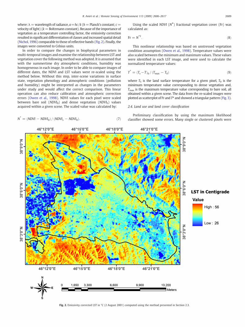
where:λ=wavelength of radiance, a=hc/k (h=Planck's constant; c=velocity of light) (k=Boltzmann constant). Because of the importance ofvegetation as a temperature controlling factor, the emissivity correctionresulted in significant differentiationof classes and increased spatial detail(Nichol, 1996) comparable to those of reflective bands (Fig. 2). Finally, theimages were converted to Celsius units.

In order to compare the changes in biophysical parameters inmulti-temporal images and examine the relationship between LST andvegetation cover the followingmethodwas adopted. It is assumed thatwith the summertime dry atmospheric conditions, humidity washomogeneous in each image. In order to be able to compare images ofdifferent dates, the NDVI and LST values were re-scaled using themethod below. Without this step, inter-scene variations in surfacestate, vegetation phenology and atmospheric conditions (pollutionand humidity) might be interpreted as changes in the parametersunder study and would affect the correct comparison. This linearoperation can also reduce calibration and atmospheric correctionerrors (Owen et al., 1998). NDVI values for each pixel were scaledbetween bare soil (NDVI0) and dense vegetation (NDVIS) valuesacquired within a given scene. The scaled value was calculated by:

N⁎ = NDVI − NDVI0ð Þ= NDVIs − NDVI0ð Þ: ð7Þ

Fig. 2. Emissivity corrected LST in °C (2 August 2001) co

Using the scaled NDVI (N⁎) fractional vegetation cover (Fr) wascalculated as:

Fr = N⁎2: ð8Þ

This nonlinear relationship was based on unstressed vegetationcondition assumption (Owen et al., 1998). Temperature values werealso scaled between theminimum andmaximum values. These valueswere identified in each LST image, and were used to calculate thenormalized temperature values:

T⁎ = Ts−Tð Þ0 = Tmax − T0ð Þ ð9Þ

where TS is the land surface temperature for a given pixel, T0 is theminimum temperature value corresponding to dense vegetation and,Tmax is the maximum temperature value corresponding to bare soil, allobtained within a given scene. The data from the re-scaled images wereplotted as scatterplot of Fr andT⁎ and showed a triangular pattern (Fig. 3).

2.4. Land use and land cover classification

Preliminary classification by using the maximum likelihoodclassifier showed some errors. Many single or clustered pixels were

mputed using the method presented in Section 2.3.

Fig. 3. Scatter plot of normalized surface radiant temperature (T⁎) vs. fractionalvegetation cover (Fr) from the Landsat 7 image with overlaid target LULC classes, 2August 2001. Fr and T⁎ values were calculated according to the Eqs. (7)–(9). The initialrange of Fr and T⁎ (between 0 and 1) was re-scaled to (0–255) due to disk space andprocessing considerations. The plus signs represent the average value of Fr and T⁎forthe LULC class mentioned on the graph. The surrounding ellipses delineate 1 standarddeviation level of Fr and T⁎ around the mean value showing their variation for eachLULC class.

2610 R. Amiri et al. / Remote Sensing of Environment 113 (2009) 2606–2617

labeled as urban classes in non-urban mountains and urban areaswere not correctly classified. Therefore, in order to eliminate thisproblem, a principal components analysis was used to reduce thepossible influence of correlations among the image bands. In addition,data of texture measured by the variance (Haralick et al., 1973) andelevation (Strahler et al., 1978) were also used as additional bands.Application of this method in the classification resulted in accuracy ofabout 70% in three datasets. A divergence matrix was used to examinethe separability of training areas and verify those areas to be used inthe classification. For the purpose of accuracy assessment, a confusionmatrix was calculated.

By using the LULC classification and surface temperature data,statistical details of each class including the average, maximum andminimum of variance were extracted (Fig. 4). Three separate thermalgroups became clear by examining the average values. Water class inall three images was about 5–9° cooler than the other classes. Thisdifferencewas due to heat transfer capability of water and the transferof energy as latent heat. The second thermal class (medium

Fig. 4. Bar chart of the surface temperature per LULC class in °C (18 August 1998).

temperature class) included green spaces and cultivation classes.This group showed a 4–5° difference with the hottest group. Thecooling mechanism of vegetation was visible as an ‘urban cool island’in hot urban areas. Built-up land use classes (residential, commercialand roads) along with bare land class formed the third group, whichdisplayed a high temperature due to the lack of evaporative coolingmechanism and low heat transfer capacity.

The range of values of temperature in each class can be related tothe heterogeneity of each class. Cultivation class showed a high rangevalue due to sub-pixel mixing of surface components such asvegetation and dry, bare soil and differences in their thermalproperties. For a more detailed study, separation of this class intoless general classes may be useful. On the other hand, the residentialclass, which mostly consisted of impervious surfaces (e.g. asphalt),showed a low range value which was an indicator of the homoge-neous construction materials and patterns used in the study area.

2.5. Temporal trajectory

The trajectory analysis was carried out in the TVX space for LULCclasses. For this purpose, based on the image classification results, thechange imagewasproduced for 1989–1998period. In the change image,areas with residential change destination were extracted (Fig. 5). Thechanges of interest were those from bare land, green space, andcultivation to residential. The change image was overlaid on the Fr andT⁎ images and the mean values of these parameters were extractedand plotted for the starting point (1989) and the end point (1998)and plotted in the TVX space. Fig. 5 shows these changes and the resultsof pixel trajectory.

3. Results

3.1. Analysis of the LST–vegetation fraction space

The TVX space was formed by plotting the parameter images in anFr vs. T⁎ scatterplot (Fig. 4). The overall distribution of the pixelsinside the space depicted the typical triangular shape observed byother authors (Lambin & Ehrlich, 1996; Owen et al., 1998; Carlson &Arthur, 2000). Three vertexes of the triangle governed the shape ofthe triangle reflecting the physical conditions of the area. The upper-left corner corresponded to the pixels representing cool conditions(high Fr and hence low T⁎) and lower-right corner was formed bypixels suffering hot conditions (low Fr, high T⁎). Fig. 4 demonstrates aclear ‘warm edge’ defined by the right side of the pixel envelope. Thewell-known inverse relationship between vegetation indices and LSToccurred in the direction of warm edge along the points where a

Fig. 5. Change trajectory in the TVX space for the long-term (1989–1998) period (30June 1989–18 August 1998). The vectors show magnitude of change associated withLULC change from green space, cultivation and barren pixels to urbanized pixels.

2611R. Amiri et al. / Remote Sensing of Environment 113 (2009) 2606–2617

decrease in Fr caused an increase in T⁎. Themajority of the pixels weredistributed in this diagonal direction, mainly based on the averagetranspiration value inside the pixels. However, the third (lower-left)corner which resulted in the triangular distribution had low T⁎despite the low Fr, implying that the cooling mechanism for thesepixels was mainly evaporation instead of transpiration. Edges of thetriangle represent the transition between the two extreme points,without being influenced by the third point. The length and the slopeof the edge imply different transition types and could result indifferent triangles. The space between vertexes and edges was amixed space (in contrast to the pure vertices), in which the proportionof existing extreme conditions inside a pixel determined the relativelocation of the pixel. The shape suggested that a full range of differentconditions existed in the study area. However, the concentration ofthe pixels and tendency of the peak values to lower Fr and higher T⁎showed that hot conditions were dominant in the study area. Themost frequent values were located between (0.63<T⁎<0.67) and(0.04<Fr<0.08), which corresponded with the dominant urban andbare land classes (Fig. 4).

To inspect the relationship between the distribution of T⁎ and Frvalues and the target LULC (residential, cultivation, green space, waterand bare soils) pixels, spectral characteristics of these classes wereextracted. The (+) sign shows the average value, with a surroundingellipse depicting 1 SD level of T⁎ and Fr for a given class (Fig. 4). Threedistinctive clusters of pixels belonging to different LULC types areapparent, which almost correspond to the vertexes of the triangle. Thelocation of a cluster of pixels belonging to a certain LULC type in thespace was related to different cooling mechanisms. Vegetated(cultivated areas, parks and fruit-tree plantations) pixels wereconcentrated in the upper-left corner and represented cool thermalconditions. This cluster consisted of two LULC types, which largelyoverlapped and shared common characteristics. A noteworthy pointwas the position of their average value inside the other class, whichshowed the difficulty of their separation in this space. The green-spacepixels (0.3<Fr<0.63) and (0.23<T⁎<0.35) mainly corresponded totwomajor sub-classes; fruit-tree plantations surrounding the city (andsome patches remaining inside the city) and ornamental trees inrecreational centers and public parks. The green-space class showedthe highest Fr variation with relatively low T⁎ variations, whichshowed itself in vertical orientation of the ellipse (Fig. 4). The diverseFr of this class was due to a different plantation architecture ofrecreational parks and fruit trees; the former occupied the upper partsof the ellipse while the latter occupied the lower parts. In the case ofthe recreational parks, trees, shrubs and grasses represented a multi-level greening and resulted in the exposure of green and cool substratewhere the trees were not dense and, therefore, occupying cool andgreen (i.e. upper) parts of the ellipse. In contrast, the lower part of theellipse was related to fruit-tree orchards (in some cases functioning asrecreational centers as well) exposing a dry, tree shadowed andrelatively hot substrate because the surface vegetationwas removed tosavewater consumedbyweeds. The exposed hot substrate of the fruit-tree class raised the aggregate surface temperature inside a pixelsharply as the trees became sparse, but sub-pixel shading mitigatedthis effect. The slope of this ellipse could be attributed to the inverserelationship between Fr and surface temperature. The cultivated pixelswere generally warmer than the green-space pixels because theyconsisted of less dense surface coverage. They also exhibited lessvegetation fraction variations (0.23<Fr<0.53) while showing aslightly higher temperature variation (0.25<T⁎<0.39). These pixelsweremainly located in thewestern fringe of the city. The considerableFr variability for this class could be attributed to the properties ofdifferent types of agricultural products cultivated and some unculti-vated patches covered with weeds. This wide range of Fr resulted inrelatively large temperature variability.

The second cluster of pixels occupied the lower-right cornerdemonstrating hot conditions. The two classes in this cluster (urban

and bare land) overlap to some extent but less than the first cluster. Thelocationof this cluster near to the peak value of distribution implied thatthe majority of pixels were those largely affected by urbanization orbelonged to a bare natural background. Small variation of Fr(00.2<Fr<0.11) showed that the green component inside these pixelsof this clusterwasnot very significant. Thiswasdue to the overall designof the city and the sparse vegetation of natural landscape. These twoclasses demonstrated homogeneous pixels and showed low tempera-ture variation due to a uniform landscape. Brick and concrete were themajor constructionmaterials, but asphalt surfacesweremore evident asthey covered most of the roads and rooftops. The sensor did not viewvertical surfaces due to the high altitude of the satellite and relativelylow height of the buildings. This condition also made the shadowingeffect insignificant in creating variability in T⁎. The urban class wasexpected to showhigher variability due to different stages and phases ofurbandevelopmentwhen it gradually expanded to green areas inside oraround the city. However, because the urbanization in these areasoccurred at the expense of irrigated green space and started byremoving the green space, semi-developed and under developmenturbanized pixels exposed bare soil, which shared similar characteristicswith urbanized pixels, and variability remained low. The temperaturevariation of bare grounds couldbeattributed to hillside shadowing. Verysparse vegetation, except for the spots where water was found, madeevapotranspiration an insignificant factor in cooling the surfacetemperature. Bare pixels were also found inside the city in pre-development pixels where vegetation cover was left without irrigation.

A few pixels associated with an artificial water body inside arecreational center in the southwestern part of the city, and wet landsbelonging mainly to the cultivation class formed the third corner ofthe triangle. High thermal capacity, and transfer of energy throughlatent heat allowed the water pixels to maintain low temperaturedespite the lack of Fr. Due to the circulation of water, the water bodywas expected to represent the most homogeneous class in terms of itsthermal variability. In fact, the water body showed relatively highvariability, which could be related to the contribution of surroundinghotter pixels especially in the edges of the water body.

The position of a cluster of pixels belonging to a certain LULC classmay be related to the human manipulation in the natural landscapeleading to different physical conditions. The semi-arid landscape ofthe area belonged to the hot conditions. The cool conditions wereachieved by planting vegetation, mainly along the lines of traditionaldesign on this hot natural background. Hot conditions were the resultof new development, through which new materials changed thesurface energy budget. The implication of this issue on design practicecould be either to use large classes of vegetated surfaces such as largeparks, or to increase green component inside each pixel to decreaseaggregate surface temperature. Based on the observations in the TVXspace, it seems that the latter seemsmore practical, which would shiftthe urban class away from bare land towards better conditions. Theplanning recommendations are only based on the analysis of thebroad LULC classes. It should be considered that there are severalother factors other than the amount of green component that canaffect the success of planning projects. For example, as mentionedbefore different architecture of the green class could result in differentsurface temperature patterns.

3.2. Temporal dynamics of the LST–vegetation fraction space

3.2.1. Temporal trajectoryChanges in biophysical conditions in each pixel under urbanization

could be traced in the Fr/T⁎ space in multi-temporal studies. Theapproach used here has some differences to the methods used byothers in similar studies, as we used LULC classes to assess the effect ofcertain types of LULC alteration, instead of geographic subsets, tocompare different development styles, as used by Carlson and Arthur(2000) and Owen et al. (1998).

2612 R. Amiri et al. / Remote Sensing of Environment 113 (2009) 2606–2617

In order to illustrate the thermal effects of certain types of LULCchange the pixel trajectory was performed. The trajectory exhibited amigration of pixels from cool and green to hot and bare conditions dueto urbanization between 1989 and 1998 (Fig. 5). The most frequentchanges were in the green-space class. These areas showed a notableincrease in surface temperature (ΔT⁎=0.27) with a decrease in Fr.The bare land class experienced the smallest changes because it was inthe similar thermal cluster as the built-up class. A noteworthy point isthe general migration trend of pixels undergoing urbanization fromcool to hot conditions. This trend was due to large vegetation losscaused by the replacement of fruit-tree plantation and green spaceswith impervious urbanized pixels. This conversion affected green-space class (i.e. orchards, fruit-tree sites and ornamental trees)substantially because it followed a large path in the space and facedconsiderable alteration in the surface climate conditions (Fig. 5).These areas were mostly located in once fringe areas of the city, andwere later changed to residential areas at the expense of cooling trees.The second class showing significant change was agriculture (Fig. 5).This class was affected by urbanization mainly in the western parts ofthe city (Fig. 6). Change path from bare land to urbanization was theabundant type of change (Fig. 6), while its change path in the TVXspace was less significant compared to green space and cultivationclasses (Fig. 5). As previously observed by Owen et al. (1998) andCarlson and Arthur (2000), pixels undergoing urbanization con-verged, and tended to concentrate in the lower right (hot condition)corner, and in the last stages of development, they becameindistinguishable as they completely lose their initial characteristics(Fig. 5). In this semi-arid region, the latest steps occurred very quicklyas the vegetation cover was maintained by irrigation and quicklychanged to natural bare lands after being abandoned.

Fig. 6. Change map for the 1989–1998 period (30 June 1989–18 August 1998). The change

3.2.2. Uncertainty in the TVX space dynamicsAs observed previously, urbanization stimulated pixel migration in

the form of vectors in the TVX space (Fig. 5). Generally, the length ofchange vector can be interpreted as the magnitude of the change.However, in fact, in addition to information about real surface alterations,these change vectors included some components of noise resulting fromnatural variations such as differences in illumination, atmospheric andsurface conditions due to different image acquisition times. Therefore, itcan be concluded that the vectors in Fig. 5 were composed of signal andnoise. In order to address the uncertainty included in the assessment ofthe urbanization effect, the noise component should be estimated. Thiswas carried out here by identifying the areas that did not undergo anyLULC changes and then these No-Change areas were used as controlpoints to assess the uncertainty involved. Ideally, if the vectorswere onlybeing controlled by LULC changes, it would be expected that themagnitude of the change vector for the No-Change areas to be equal tozero, but in reality, above-mentioned noise factors could affect the pixelsand result in values above zero. Ourfirst premisewas that themagnitudeof the changevector in theNo-Changeareaswasdue to factors other thanthe changes in LULC type (noise component). The second premise wasthe assumption that the inter-scene variation (noise factor) affects bothChange andNo-Change classes of certain LULC type by the same amount.Therefore, the amount of noise can be extracted from No-change classesand be used to separate noise component from change vector. These twopremises were the basis for adopting the following methodology. Inaddition,wehypothesized that thenoise effect is nothomogeneousbut isclass-dependant.

By using LULC classificationmaps and excluding cloud coverage areas,change maps of target change types were produced for the 1989–98 and1998–2001 periods (Figs. 6 and 7). From the change maps, unchanged

map highlights the pixels changed from barren, green space and agriculture to urban.

Fig. 7. Change map for the 1998–2001 period (18 August 1998–2 August 2001). The change map highlights the pixels changed from barren, green space and agriculture to urban.

2613R. Amiri et al. / Remote Sensing of Environment 113 (2009) 2606–2617

areas for bare land, agriculture, and green space for the two periods wereidentified as the change from these classes tourbanwere addressed in thetrajectory analysis. From the No-Change areas in 1989, 1998 and 2001images, average values of Fr and T⁎ for bare land, agriculture and green-space target classeswere extracted separately. Owen et al. (1998) used anaverage value of all unchanged pixels as the control point. In anotherstudy, Carlson and Arthur (2000) used the average value of the wholeimages as the control point in theTVXspace.Here,weusedaveragevaluesfor each individual classes involved in the analysis. Using the averagevalues of Fr and T⁎ for the starting and end point of the two periods(1989–1998 and1998–2001) a change vectorwas computed for eachNo-change class. The magnitude of these change vectors computed for eachNo-Change type (barren–barren, agricultural–agricultural and greenspace–green space) were regarded as the threshold values for separationof Change fromNo-Change for a particular class. A change vectorwas alsocomputed for each change class using the average values of Fr and T⁎. The

Table 1The statistics for the changes to urban land use between 1989–1998 period.

LULC class Magnitude ofchange vectora

Population SD(individual vectors)

1989 1998

Barren Barren 20.30b 12.80Barren Urban 28.93 16.19Green space Green space 56.47b 26.06Green space Urban 79.27 37.03Agriculture Agriculture 72.02b 36.94Agriculture Urban 78.40 46.77

a The magnitude of change vectors was calculated using the beginning and endvalues of Fr and T⁎ averaged inside LULC classes.

b These values were used as the threshold values in the uncertainty analysis.

threshold and change values are shown in Table 1 for 1989–1998 periodand in Table 2 for 1998–2001 period. The magnitude of the thresholdvectors for No-Change classes in Table 1 were less than the magnitude ofthe average change vector for change classes implying relatively lowuncertainty in this long-term period.

In contrast, according to Table 2, the magnitude of the thresholdvector computed for the three No-Change classes (barren, urban andgreen space) exceeds themagnitude of the average vector of the changeclass (barren–urban, agricultural–urban, and green space–urban) forthe 1998–2001 short-term period. This means that the majority of thepixels in these changed areas probably did not undergo significantchanges but were considered as changed by the trajectory analysis.

To demonstrate the uncertainty involved in the estimation of theeffects of the target LULC changes on temperature and greennessusing the trajectory for each pixel, a change vector was computed foreach pixel (Figs. 8 and 9) and used in the following analysis. Standard

Table 2The statistics for the changes to urban land use between 1998–2001 period.

LULC class Magnitude of thechange vectora

Population SD(individual vectors)

1998 2001

Barren Barren 25.01b 12.53Barren Urban 18.24 8.51Green space Green space 35.15b 21.42Green space Urban 34.32 19.34Agriculture Agriculture 47.99b 33.32Agriculture Urban 34.50 24.45

a The magnitude of change vectors was calculated using the beginning and endvalues of Fr and T⁎ averaged inside LULC classes.

b These values were used as the threshold values in the uncertainty analysis.

Fig. 8. Change magnitude map for the long-term (1989–1998) period (30 June 1989–18 August 1998). The change vectors were computed for each pixel based on their initial (1989)and final (1998) values of Fr and T⁎ in the TVX space.

Fig. 9. Change magnitude map for the short-term (1998–2001) period (18 August 1998–2 August 2001). The change vectors were computed for each pixel based on their initial(1998) and final (2001) values of Fr and T⁎ in the TVX space.

2614 R. Amiri et al. / Remote Sensing of Environment 113 (2009) 2606–2617

2615R. Amiri et al. / Remote Sensing of Environment 113 (2009) 2606–2617

deviation of the change vectors for all Change and No-Change classeswas computed using the change vector images and is shown inTables 1 and 2. The SD values for the 1989–1998 period showed largedispersion of vector magnitudes, which could be related to theuncertainty involved. In contrast, the SD values of the 1989–98 periodshowed little variation possibly due to the shorter period of the

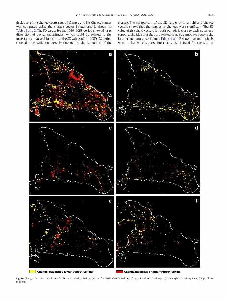
Fig. 10. Changed and unchanged areas for the 1989–1998 period (a, c, d) and for 1998–2001to urban.

change. The comparison of the SD values of threshold and changevectors shows that the long-term changes were significant. The SDvalue of threshold vectors for both periods is close to each other andsupports the idea that they are related to noise component due to theinter-scene natural variations. Tables 1 and 2 show that more pixelswere probably considered incorrectly as changed for the shorter

period (b, d, f). a, b) Bare land to urban; c, d) Green space to urban; and e, f) Agriculture

2616 R. Amiri et al. / Remote Sensing of Environment 113 (2009) 2606–2617

period of 1998–2001. It could be concluded from these results that theLULC changes depicted more significant effects for the long-term(1989–1998) period as compared to the short-term (1998–2001)period in the TVX space. The majority of the short-term changes couldbe due to natural variations, which may be attributed to vegetationphenology, different growth seasons, farming style and imageacquisition times.

Fig. 10 shows the uncertainty analysis of the TVX for the bothperiods by applying the threshold values. These images wereproduced by applying the threshold values from Tables 1 and 2 tothe change vectors for changes from bare land, green space andagriculture to urban classes addressed in the TVX space. The changevector magnitudes for the pixel positions less than the mentionedthreshold values for each class were labeled as No-Change in theimage space. Fig. 10 shows the areas with real change areas, as well asno-change areas, which due to uncertainty were considered aschanged areas. In some cases, the results showed that the majorityof the changes were really the effect of the noise component (e.g. 10band 10f). The examination of the images suggests that the uncertaintywas dependant on the LULC change type. For example, the changefrom bare land to urban LULC class involved more uncertainty thanthe other change types probably because they belonged to the samecluster and shared similar characteristics (Fig. 10a). The results implythat although an effort had been made to reduce the naturalvariability of the images and to increase comparability by means ofnormalization, there was still some uncertainty involved in the resultsand therefore all the changes could not be considered as real changes.There is a need to consider the effect of the uncertainty involved in theinterpretation of the results. The class-dependant nature of theuncertainty prompts for the need to address this issue for individualclasses. The results also imply that using an average value of thewholescene as the control point, as used in other studies, was not especiallyefficient in the study area. In addition, the second method ofestablishing the control point by averaging a certain class (e.g.agriculture) could not fully address the uncertainty of all class becausethe uncertainty showed a class-dependant nature.

4. Discussion and conclusions

In this paper, we have examined the spatial and temporaldynamics of LST in relation to LULC change in the TVX space byusing Landsat thermal IR and reflective data. Results showed that, ifapplied over relatively long periods, the adopted methodology mightbe applied to detect and monitor urban expansion and to trace thechanges in biophysical parameters such as NDVI and LST due to LULCchanges.

The construction of TVX space by normalizing the land surfacetemperature and vegetation index data provided comparabilitybetween temperature and vegetation datasets of different dates inmulti-temporal studies of the urban environment. The TVX space isuseful in providing a view of the relationship between LST, NDVI, andLULC classes. This space is also useful in monitoring changes in theseparameters and their interplay, as observed in pixel migration. Themagnitude and the direction of the movement are defined by the typeof change.

The analysis of the distribution of pixels in the TVX space showedthat dominant environmental conditions in the study area were hotand dry. This was observed by the association between thedistribution peak and the urbanized and barren pixels in hot–drycorner of the TVX space. Traditional human surface alteration createdthe cool–green edge by irrigated plantations inside the old city and itsperipherals and cool–wet edge by creating water bodies. This createddifferent surface climatic conditions, which resulted in the typicaltriangular distribution in this semi-arid environment. Recent devel-opments have changed these conditions by vast LULC changes,alterations in surface conditions and introduction of new materials.

In order to study these effects, a temporal analysis of the TVX spacewas carried out.

The temporal analysis of the TVX space showed that urbanizationresulted in the migration of pixels from cool to hot surface conditions,which is consistent with the observations by other authors (e.g., Owenet al., 1998; Carlson and Arthur, 2000). The extent of pixel migrationimplied the effect of urbanization in deterioration of environmentalquality in the form of changes in surface thermal conditions in theurban areas. The larger path, followed by the green-space pixels in theTVX space as they changed to urbanized pixels, showed that LULCchange from green space to urban caused the largest change in surfacetemperature conditions. Our results showed that in the late stages ofurbanization, affected pixels tended to converge and entirely losetheir initial characteristics in the TVX space. In contrast with Carlsonand Arthur (2000), this study employed a different approach in thetrajectory analysis by using original pixel size instead of aggregatedpixels. In addition, we used LULC classes instead of geographicalsubsets as the unit of analysis.

These modifications in the methodology allowed us to investigatethe effect of specific LULC change type on LST and to assess theuncertainty in the TVX space. The analysis of the uncertainty involvedin the temporal analysis showed that the method used to create anormalized TVX space did not remove the effect of inter-scenevariability. There were a certain number of unchanged pixelsmistakenly regarded as changed pixels. Our results showed that theamount of uncertainty was class-dependent. This finding suggestedthat the selection of an average of Fr and T⁎ for the whole scene ascontrol point could not fully remove the inter-scene variability. Inaddition, the selection of an un-altered patch of land as control pointswas not very effective as well due to the same class-dependent natureof uncertainty in the space. Themethod developed here can be used toremove uncertainty by selection of multiple control points from eachLULC classes. The next step in the analysis of uncertainty could be theuse of spectral mixture analysis to assess the effect of differentcompositions of LULC inside the pixels in the migration of pixels andthe uncertainty involved. It seems that spectral mixture analysis couldbe promising in gaining better insight to the mixed TVX space and itsinternal composition and by providing information on changes insurface climatic conditions (e.g., Weng & Lu, 2009).

The comparison of long-term changes against short-term changesalso had implications for this research. The noise component showedmore or less comparable effects on both periods. This supports theassumption in our method to consider the magnitude of no-changevectors as the noise component to separate it from the change vector.On the other hand, it showed that the noise component should beaddressed for both long-term and short-term changes. The impor-tance of this issue becomes more critical for the short-term period asthemajority of the observed change could be due to the effect of noise.This allows us to separate the real change component from the noisecomponent instead of regarding the whole change as insignificant forthe short-term period.

A possible application of the TVX space and the analysis carried outhere could be the assessment of the consequences of current andfuture LULC changes associated with urbanization on the surfacethermal environment of a city. In the case of the Tabriz urban area, theplanned or unplanned changes resulted in the alteration of the coolersurface condition established by traditional designs to hotter ones.This trend was observed by the diagonal migration of the pixels to thehotter corner of the triangular envelope inside the TVX space. Theinitial condition of migrated pixels was observed as the amount of Frand type of LULC and associated surface temperature in the TVX space.This observation has the potential to assist informed LULC planningdecisions to control changes in surface characteristics in order tomodify surface climate by establishing the conditions close to initialones for each pixel. According to Fig. 5, vegetation could serve as agood remedy for the adverse warming surfaces, which is embraced by

2617R. Amiri et al. / Remote Sensing of Environment 113 (2009) 2606–2617

the traditional urban designs. The increase in the fraction of vegetatedsurface inside a pixel could stop the current migration trend andstimulate the migration of the pixels in the opposite direction in theTVX space. Nevertheless, in case of the green-space classes, it wasobserved that the variations in the structure and design of the greenspace could result in slightly different surface thermal conditions. Themulti-level design of the recreational parks created cooler surfacesthan the orchards. In addition, the expansion of the city in barrenlands could cause less surface temperature alterations as theurbanized and barren pixels showed very close characteristics in theTVX space.

References

Artis, D. A., & Carnahan, W. H. (1982). Survey of emissivity variability in thermographyof urban areas. Remote Sensing of Environment, 12, 313−329.

Carlson, T. N. (2007). An overview of the so-called “Triangle Method” for estimatingsurface evapotranspiration and soil moisture from satellite imagery. Sensors, 7,1612−1629.

Carlson, T. N., & Arthur, S. T. (2000). The impact of land use— land cover changes due tourbanization on surface microclimate and hydrology: A satellite perspective. Globaland Planetary Change, 25, 49−65.

Carlson, T. N., & Sanchez-Azofeifa, G. A. (1999). Satellite remote sensing of land usechanges in and around San José, Costa Rica. Remote Sensing of Environment, 70(3),247−256.

Carlson, T. N., Gillies, R. R., & Perry, E. M. (1994). A method to make use of thermalinfrared temperature and NDVI measurements to infer surface water content andfractional vegetation cover. Remote Sensing Reviews, 9, 161−173.

Chen, X. L., Zhao, H. M., Li, P. X., & Yin, Z. Y. (2006). Remote sensing image-basedanalysis of the relationship between urban heat island and land use/cover changes.Remote Sensing of Environment, 104(2), 133−146.

Dousset, B., & Gourmelon, F. (2003). Satellite multi-sensor data analysis of urbansurface temperature and land cover. ISPRS Journal of Photogrammetry and RemoteSensing, 58, 43−54.

Eastman, R. J. (1999). Idrisi guide to GIS and image processing. Clark University.Gallo, K. P., & Tarpley, J. D. (1996). The comparison of vegetation index and surface

temperature composites for urban heat island analysis. International Journal ofRemote sensing, 17, 3071−3076.

Gillies, R. R., Carlson, T. N., Cui, J., Kustas, W. P., & Humes, K. S. (1997). A verification ofthe ‘triangle’ method for obtaining surface soil water content and energy fluxesfrom remote measurements of the normalized difference vegetation index (NDVI)and surface temperature. International Journal of Remote Sensing, 18, 3145−3166.

Goward, S. N., Xue, Y., & Czajkowski, K. P. (2002). Evaluating land surface moistureconditions from the remotely sensed temperature/vegetation index measure-ments: An exploration with the simplified biosphere model. Remote Sensing ofEnvironment, 79, 225−242.

Haralick, R., Shanmugan, K., & Dinstein, I. (1973). Textural features for imageclassification. IEEE Transactions on Systems, Man and Cybernetics, 3, 610−621.

Iranian Census Center (2007). Iranian cities population.Jiang, L., & Islam, S. (2001). Estimation of surface evaporation map over southern Great

Plains using remote sensing data. Water Resources Research, 37(2), 329−340.Jimenes-Munoz, J. C., & Sobrino, J. A. (2003). A generalized single-channel method for

retrieving land surface temperature from remote sensing data. Journal ofGeophysical Research, 108. doi:10.1029/2003JD003480

Kustas, W. P., Norman, J. M., Anderson, M. C., & French, A. N. (2003). Estimating subpixelsurface temperatures and energy fluxes from the vegetation index-radiometrictemperature relationship. Remote sensing of Environment, 85, 429−440.

Lambin, F. F., & Ehrlich, D. (1996). The surface temperature–vegetation index space forland use and land cover change analysis. International Journal of Remote Sensing, 17,463−487.

Landsat 7 science data user handbook. Available online: http://landsathandbook.gsfc.nasa.gov/handbook.html. Last accessed July 15, 2009.

Malaret, E., Bartolocci, L. A., Lozano, D. F., Anuta, P. E., &McGillem, C. P. (1985). Landsat 4and Landsat 5 thematic mapper data quality analysis. Photogrammetric Engineeringand Remote Sensing, 51, 1407−1416.

Moran, M. S., Clarke, T. R., Inoue, Y., & Vidal, A. (1994). Estimating crop water deficitusing the relation between surface–air temperature and spectral vegetation index.Remote Sensing of Environment, 49, 246−263.

Nemani, R. R., & Running, S. W. (1989). Estimation of Regional Surface Resistance toEvapotranspiration from NDVI and Thermal-IR AVHRR Data. Journal of AppliedMeteorology, 28, 276−284.

Nichol, J. E. (1994). A GIS-based approach to microclimate monitoring in Singapore'shigh-rise housing estates. Photogrammetric Engineering and Remote Sensing, 60,1225−1232.

Nichol, J. E. (1996). High-resolution surface temperature patterns related to urbanmorphology in a tropical city: A satellite-based study. Journal of AppliedMeteorology, 35, 135−146.

Nichol, J. E. (2005). Remote sensing of urban heat islands by day and night. Photo-grammetric Engineering and Remote Sensing, 71, 613−623.

Nishida, K., Nemani, R. R., Glassy, J. M., & Running, S. W. (2003). Development of anevapotranspiration index from Aqua/MODIS for monitoring surface moisturestatus. IEEE Transactions on Geoscience and Remote Sensing, 41(2), 493−501.

Owen, T. W., Carlson, T. N., & Gillies, R. R. (1998). Assessment of satellite remotely-sensed land cover parameters in quantitatively describing the climatic effect ofurbanization. International Journal of Remote sensing, 19, 1663−1681.

Pongracz, R., Bartholy, J., & Dezso, Z. (2006). Remotely sensed thermal informationapplied to urban climate analysis. Advance in Space Research, 37, 2191−2196.

Price, J. C. (1990). Using spatial context in satellite data to infer regional scaleevapotranspiration. IEEE Transactions on Geoscience and Remote Sensing, 28,940−948.

Qin, Z., Karnielli, A., & Berliner, P. (2001). A mono-window algorithm for retrieving alndsurface temperature from Landsat TM data and its application to the Israel–Egyptborder region. International Journal of Remote Sensing, 22(18), 3719−3746.

Quattrochi, D. A., & Luvall, J. C. (2004). Thermal remote sensing in land surface processes.CRC Press 440 pp.

Rao, P. K. (1972). Remote sensing of urban heat islands from an environmental satellite.Bulletin of the American Meteorological Society, 53, 647−648.

Ridd, M. K. (1995). Exploring a V–I–S _vegetation–impervious surface–soil. model forurban ecosystem analysis through remote sensing: Comparative anatomy for cities.International Journal of Remote Sensing, 16, 2165−2185.

Sobrino, J. A., Jimenez-Munoz, J. C., & Paolini, L. (2004). Land surface temperatureretrieval from Landsat TM 5. Remote Sensing of Environment, 90, 434−440.

Sandholt, I., Rasmussen, K., & Andersen, J. (2002). A simple interpretation of the surfacetemperature/vegetation index space for assessment of surface moisture status.Remote Sensing of Environment, 79, 213−224.

Smith, R. C. G., & Choudhury, B. J. (1991). Analysis of normalized difference and surfacetemperature observations over southeastern Australia. International Journal ofRemote Sensing, 12(10), 2021−2044.

Strahler, A. H., Logan, T. L., & Bryant, N. A. (1978). Improving forest cover classificationfrom Landsat by incorporating topographic information. 12th InternationalSymposium on Remote Sensing of Environment, Manila, Philippines (pp. 927−942).

Streutker, D. R. (2003). Satellite-measured growth of the urban heat island of Houston,TX. Remote Sensing of Environment, 85, 282−289.

Voogt, J. A., & Oke, T. R. (2003). Thermal remote sensing of urban climate. RemoteSensing of Environment, 86, 370−384.

Weng, Q. (2001). A remote sensing-GIS evaluation of urban expansion and its impactson surface temperature in the Zhujiang delta, China. International Journal of RemoteSensing, 22, 1999−2014.

Weng, Q. (2009). Thermal infrared remote sensing for urban climate and environ-mental studies: Methods, applications, and trends. ISPRS Journal of Photogrammetryand Remote Sensing, 64(4), 335−344.

Weng, Q., & Lu, D. (2009). Landscape as a continuum: An examination of the urbanlandscape structures and dynamics of Indianapolis city, 1991–2000. InternationalJournal of Remote Sensing, 30, 2547−2577.

Weng, Q., Lu, D., & Schubring, J. (2004). Estimation of land surface temperature–vegetation abundance relationship for urban heat island studies. Remote sensing ofEnvironment, 89, 467−483.