spatial query languages - wordpress.com · 2008-07-05 · “runall” 2002/5/29 page 52 chapter 3...

“runall”2002/5/29page 52

�

�

�

�

�

�

�

�

C H A P T E R 3

Spatial Query Languages

3.1 STANDARD DATABASE QUERY LANGUAGES

3.2 RA

3.3 BASIC SQL PRIMER

3.4 EXTENDING SQL FOR SPATIAL DATA

3.5 EXAMPLE QUERIES THAT EMPHASIZE SPATIAL ASPECTS

3.6 TRENDS: OBJECT-RELATIONAL SQL

3.7 SUMMARY

3.8 APPENDIX: STATE PARK DATABASE

A query language, the principal means of interaction with the database, is a core re-quirement of a DBMS. A popular commercial query language for relational databasemanagement systems (RDBMS) is SQL. It is partly based on the formal query language,relational algebra (RA) and it is easy to use, intuitive, and versatile. Because SDBMSsare an example of an extensible DBMS and deal with both spatial and nonspatial data,it is natural to seek for an extension of SQL to incorporate spatial data.

As shown in the previous chapter, the relational model has limitations in effectivelyhandling spatial data. Spatial data is “complex,” involving a melange of polygons, lines,and points, and the relational model is geared for dealing with simple data types such asintegers, strings, dates, and so forth.

Constructs from object-oriented programming, such as user-defined types and dataand functional inheritance, have found immediate applications in the modeling of complexdata. The widespread use of the relational model and SQL for applications involvingsimple datatypes combined with the functionality of the object-oriented model has led tothe birth of a new “hybrid” paradigm for database management systems, the OR-DBMS.

A corollary to this newfound interest in OR-DBMS is the desire to extend SQLwith object functionality. This effort has materialized into a new OR-DBMS standard forSQL:SQL3. Because we are dealing with spatial data, we examine the spatial extensionsand libraries for SQL3.

A unique feature of spatial data is that the “natural” medium of interaction withthe user is visual rather than textual. Hence any spatial query language should supporta sophisticated graphical-visual component. Having said that, we focus here on the non-graphical spatial extensions of SQL. In Section 3.1, we introduce the World database,which will form the basis of all query examples in the chapter. Sections 3.2 and 3.3 pro-vide a brief overview of RA and SQL, respectively. Section 3.4 is devoted to a discussionon the spatial requirements for extending SQL. We also introduce the OGIS standard for

52


�

�

�

�

�

�

�

�

Section 3.1 Standard Database Query Languages 53

extending SQL for geospatial data. In Section 3.5, we show how common spatial queriescan be posed in OGIS extended SQL. In Section 3.6, we introduce SQL3 and Oracle8’simplementation of a subset of SQL3.

3.1 STANDARD DATABASE QUERY LANGUAGES

Users interact with the data embedded in a DBMS using a query language. Unliketraditional programming languages, database query languages are relatively easy to learnand use. In this section we describe two such query languages. The first, RA, is themore formal of the two and typically not implemented in commercial databases. Theimportance of RA lies in the fact that it forms the core of SQL, the most popular andwidely implemented database query language.

3.1.1 World Database

We introduce RA and SQL with the help of an example database. We introduce a newexample database here to provide some diversity in examples and exercises. The World

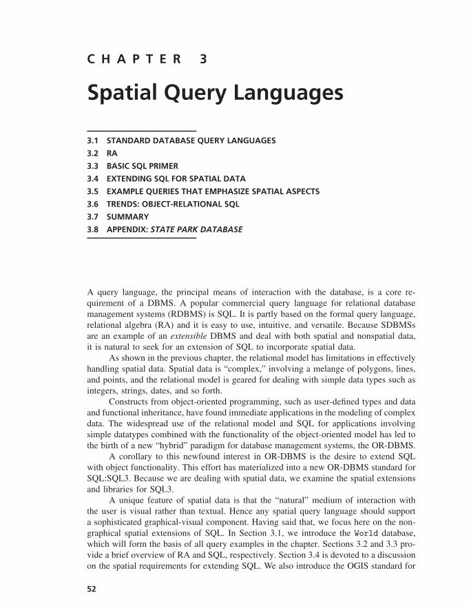
database consists of three entities: Country, City, and River. The pictogram-enhancedER diagram of the database and the example tables are shown in Figure 3.1 and Table 3.1,respectively. The schema of the database is shown below. Note that an underlined at-tribute is a primary key. For example, Name is a primary key in Country table, Citytable, and River table.

Country(Name: varchar(35), Cont: varchar(35), Pop: integer,

GDP:Integer, Life-Exp: integer, Shape:char(13))City(Name: varchar(35), Country: varchar(35), Pop: integer,

Capital:char(1), Shape:char(9))River(Name: varchar(35), Origin: varchar(35), Length: integer,

Shape:char(13))

POPULATION

CAPITAL

ORIGINATESCOUNTRY RIVERCITY

NAME

CAPITAL-OF

NAME

POPULATION

LIFE-EXP

NAMELENGTH

CONTINENT

GDP

FIGURE 3.1. The ER diagram of the World database.


�

�

�

�

�

�

�

�

54 Chapter 3 Spatial Query Languages

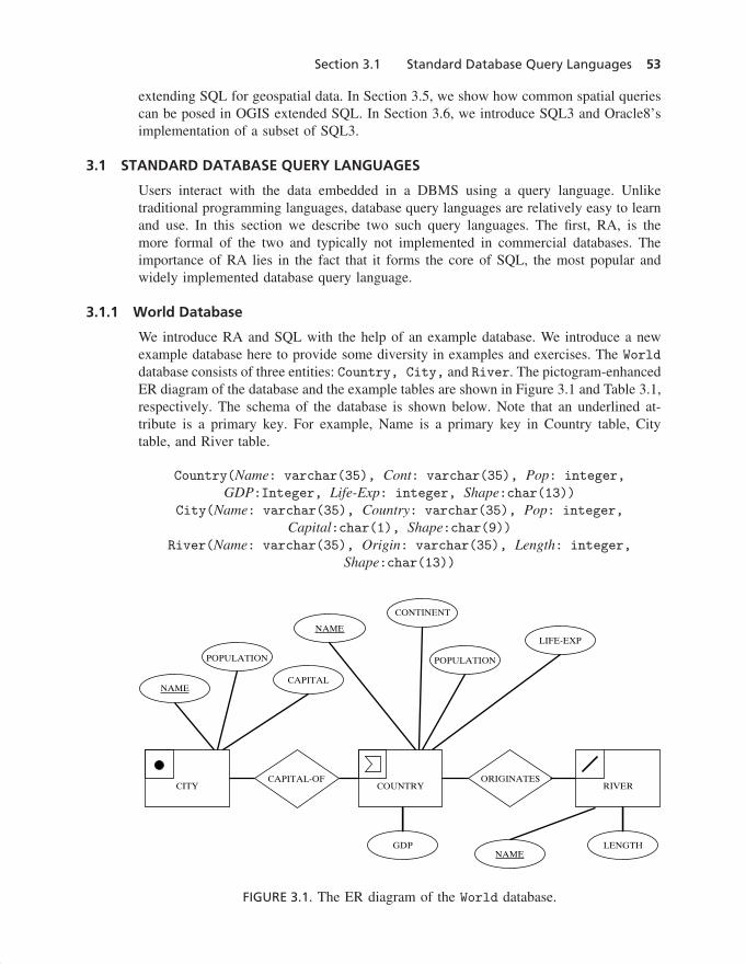
TABLE 3.1: The Tables of the World Database with Sample Records

COUNTRY Name Cont Pop (millions) GDP (billions) Life-Exp ShapeCanada NAM 30.1 658.0 77.08 Polygonid-1Mexico NAM 107.5 694.3 69.36 Polygonid-2Brazil SAM 183.3 1004.0 65.60 Polygonid-3Cuba NAM 11.7 16.9 75.95 Polygonid-4USA NAM 270.0 8003.0 75.75 Polygonid-5

Argentina SAM 36.3 348.2 70.75 Polygonid-6

(a) Country

CITY Name Country Pop (millions) Capital ShapeHavana Cuba 2.1 Y Pointid-1

Washington, D.C. USA 3.2 Y Pointid-2Monterrey Mexico 2.0 N Pointid-3

Toronto Canada 3.4 N Pointid-4Brasilia Brazil 1.5 Y Pointid-5Rosario Argentina 1.1 N Pointid-6Ottawa Canada 0.8 Y Pointid-7

Mexico City Mexico 14.1 Y Pointid-8Buenos Aires Argentina 10.75 Y Pointid-9

(b) City

RIVER Name Origin Length (kilometers) ShapeRio Parana Brazil 2600 LineStringid-1

St. Lawrence USA 1200 LineStringid-2Rio Grande USA 3000 LineStringid-3Mississippi USA 6000 LineStringid-4

(c) River

The Country entity has six attributes. The Name of the country and the continent(Cont) it belongs to are character strings of maximum length thirty-five. The population(Pop) and the gross domestic product (GDP) are integer types. The GDP is the totalvalue of goods and services produced in a country in one fiscal year. Life-Exp attributerepresents the life expectancy in years (rounded to the nearest integer) for residents ofa country. The Shape attribute needs some explanation. The geometry of a country isrepresented in the Shape column of Table 3.1. In relational databases, where the datatypesare limited, the Shape attribute is a foreign key to a shape table. In an object-relational orobject-oriented database, the Shape attribute will be a polygon abstract datatype (ADT).Because, for the moment, our aim is to introduce basic RA and SQL, we will not querythe Shape attribute until Section 3.4.

The City relation has five attributes: Name, Country, Pop, Capital, and Shape. TheCountry attribute is a foreign key into the Country table. Capital is a fixed charactertype of length one; a city is a capital of a country, or it is not. The Shape attribute is aforeign key into a point shape table. As for the Country relation, we will not query theShape column before learning about OGIS data types for SQL3.

The four attributes of the River relation are Name, Origin, Length, and Shape. TheOrigin attribute is a foreign key into the Country relation and specifies the country where


�

�

�

�

�

�

�

�

Section 3.2 RA 55

the river originates. The Shape attribute is a foreign key into a line string shape table.To determine the country of origin of a river, the geometric information specified in theShape attribute is not sufficient. The overloading of name across tables can be resolvedby a qualifying attribute with tables using a dot notation table.attribute. County.Name,city.Name, and river.Name uniquely identify the Name attribute inside different tables.We also need information about the direction of the river flow. In Chapter 7 we discussquerying spatial networks where directional information is important.

3.2 RA

RA is a formal query language associated with the relational model. An algebra is amathematical structure consisting of two distinct sets of elements, (�a,�o). �a is the setof operands and �o is the set of operations. An algebra must satisfy many axioms, butthe most crucial is that the result of an operation on an operand must remain in �a . Asimple example of an algebra is the set of integers. The operands are the integers, andthe operations are addition and multiplication. In Chapter 8 we discuss other kinds ofalgebra associated with raster and image objects.

In RA there is only one type of operand and six basic operations. The operand is arelation (table), and the six operations are select, project, union, cross-product, difference,and intersection. We now introduce some of the basic operations in detail.

3.2.1 The Select and Project Operations

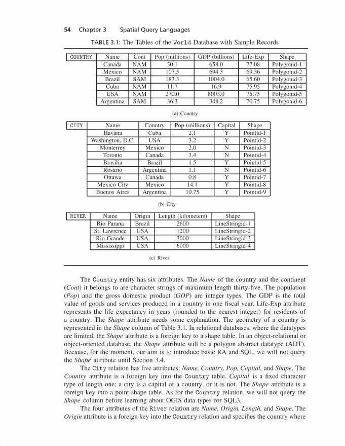
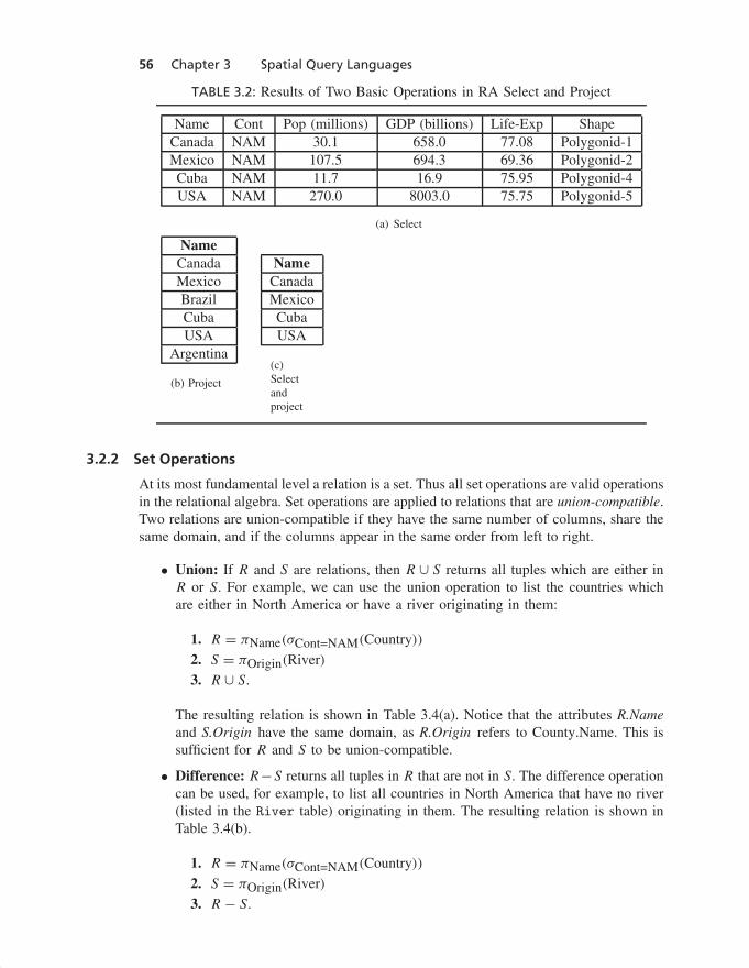
To manipulate data in a single relation, RA provides two operations: select and project.The select operation retrieves a subset of rows of the relational table, and the projectoperation extracts a subset of the columns. For example, to list all the countries in theCountry table which are in North-America (NAM), we use the following relationalalgebra expression:

σcont=NAM(Country).

The result of this operation is shown in Table 3.2(a). The rows retrieved by theselect operation σ are specified by the comparison selection operator, which in thisexample is cont=‘North-America’. The schema of the input relation is not altered by theselect operator. The formal syntax of the select operation is

σ<selection operator >(Relation).

Subsets of columns for all rows in a relation are extracted by applying the projectoperation, π . For example, to retrieve the names of all countries listed in the Country

table, we use the following expression:

πName(Country).

The formal syntax of the project operation is

π< list of attributes >(Relation)

We can combine the select and the project operations. The following expressionyields the names of countries in North America. See Table 3.2(c) for the result.

πName(σCont=NAM(Country))


�

�

�

�

�

�

�

�


TABLE 3.2: Results of Two Basic Operations in RA Select and Project

Name Cont Pop (millions) GDP (billions) Life-Exp ShapeCanada NAM 30.1 658.0 77.08 Polygonid-1Mexico NAM 107.5 694.3 69.36 Polygonid-2Cuba NAM 11.7 16.9 75.95 Polygonid-4USA NAM 270.0 8003.0 75.75 Polygonid-5

(a) Select

NameCanadaMexicoBrazilCubaUSA

Argentina

(b) Project

NameCanadaMexicoCubaUSA

(c)Selectandproject

3.2.2 Set Operations

At its most fundamental level a relation is a set. Thus all set operations are valid operationsin the relational algebra. Set operations are applied to relations that are union-compatible.Two relations are union-compatible if they have the same number of columns, share thesame domain, and if the columns appear in the same order from left to right.

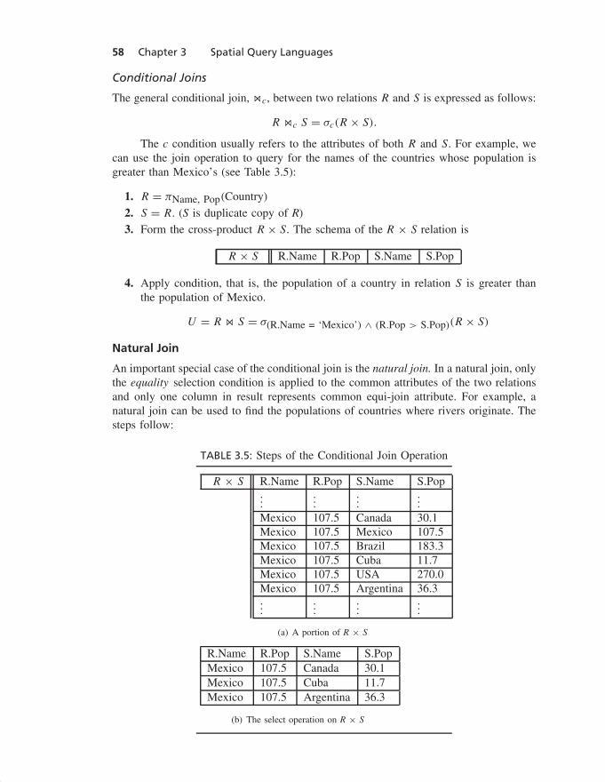
• Union: If R and S are relations, then R ∪ S returns all tuples which are either inR or S. For example, we can use the union operation to list the countries whichare either in North America or have a river originating in them:

1. R = πName(σCont=NAM(Country))

2. S = πOrigin(River)

3. R ∪ S.

The resulting relation is shown in Table 3.4(a). Notice that the attributes R.Nameand S.Origin have the same domain, as R.Origin refers to County.Name. This issufficient for R and S to be union-compatible.

• Difference: R−S returns all tuples in R that are not in S. The difference operationcan be used, for example, to list all countries in North America that have no river(listed in the River table) originating in them. The resulting relation is shown inTable 3.4(b).

1. R = πName(σCont=NAM(Country))

2. S = πOrigin(River)

3. R − S.


�

�

�

�

�

�

�

�

Section 3.2 RA 57

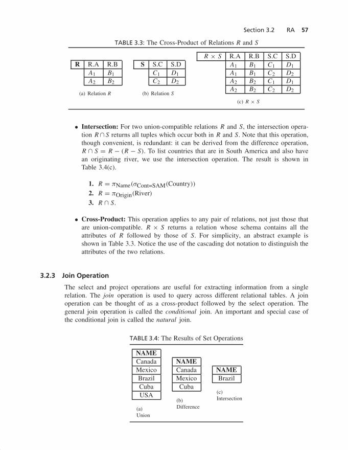
TABLE 3.3: The Cross-Product of Relations R and S

R R.A R.BA1 B1A2 B2

(a) Relation R

S S.C S.DC1 D1C2 D2

(b) Relation S

R × S R.A R.B S.C S.DA1 B1 C1 D1A1 B1 C2 D2A2 B2 C1 D1A2 B2 C2 D2

(c) R × S

• Intersection: For two union-compatible relations R and S, the intersection opera-tion R∩S returns all tuples which occur both in R and S. Note that this operation,though convenient, is redundant: it can be derived from the difference operation,R ∩ S = R − (R − S). To list countries that are in South America and also havean originating river, we use the intersection operation. The result is shown inTable 3.4(c).

1. R = πName(σCont=SAM(Country))

2. R = πOrigin(River)

3. R ∩ S.

• Cross-Product: This operation applies to any pair of relations, not just those thatare union-compatible. R × S returns a relation whose schema contains all theattributes of R followed by those of S. For simplicity, an abstract example isshown in Table 3.3. Notice the use of the cascading dot notation to distinguish theattributes of the two relations.

3.2.3 Join Operation

The select and project operations are useful for extracting information from a singlerelation. The join operation is used to query across different relational tables. A joinoperation can be thought of as a cross-product followed by the select operation. Thegeneral join operation is called the conditional join. An important and special case ofthe conditional join is called the natural join.

TABLE 3.4: The Results of Set Operations

NAMECanadaMexicoBrazilCubaUSA

(a)Union

NAMECanadaMexicoCuba

(b)Difference

NAMEBrazil

(c)Intersection


�

�

�

�

�

�

�

�


Conditional Joins

The general conditional join, ��c, between two relations R and S is expressed as follows:

R ��c S = σc(R × S).

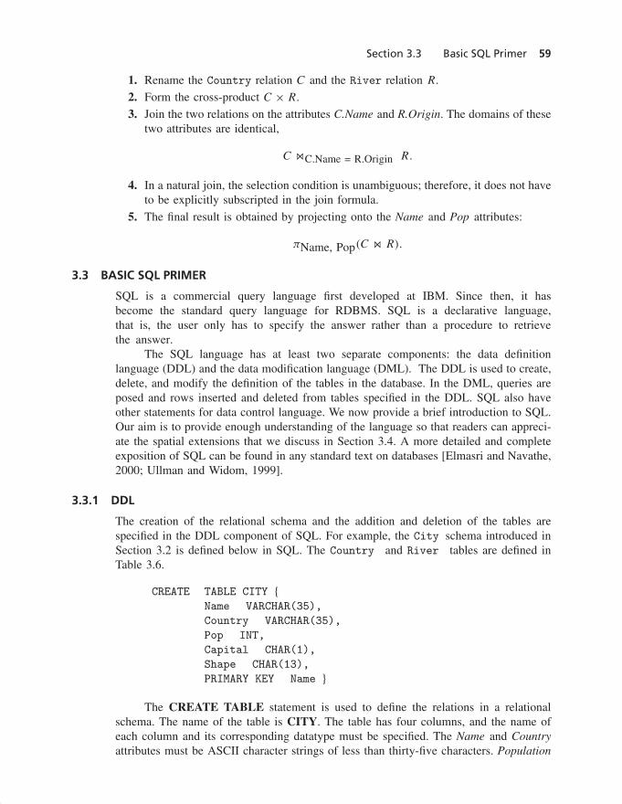
The c condition usually refers to the attributes of both R and S. For example, wecan use the join operation to query for the names of the countries whose population isgreater than Mexico’s (see Table 3.5):

1. R = πName, Pop(Country)

2. S = R. (S is duplicate copy of R)

3. Form the cross-product R × S. The schema of the R × S relation is

R × S R.Name R.Pop S.Name S.Pop

4. Apply condition, that is, the population of a country in relation S is greater thanthe population of Mexico.

U = R �� S = σ(R.Name = ‘Mexico’) ∧ (R.Pop > S.Pop)(R × S)

Natural Join

An important special case of the conditional join is the natural join. In a natural join, onlythe equality selection condition is applied to the common attributes of the two relationsand only one column in result represents common equi-join attribute. For example, anatural join can be used to find the populations of countries where rivers originate. Thesteps follow:

TABLE 3.5: Steps of the Conditional Join Operation

R × S R.Name R.Pop S.Name S.Pop...

......

...

Mexico 107.5 Canada 30.1Mexico 107.5 Mexico 107.5Mexico 107.5 Brazil 183.3Mexico 107.5 Cuba 11.7Mexico 107.5 USA 270.0Mexico 107.5 Argentina 36.3...

......

...

(a) A portion of R × S

R.Name R.Pop S.Name S.PopMexico 107.5 Canada 30.1Mexico 107.5 Cuba 11.7Mexico 107.5 Argentina 36.3

(b) The select operation on R × S


�

�

�

�

�

�

�

�

Section 3.3 Basic SQL Primer 59

1. Rename the Country relation C and the River relation R.

2. Form the cross-product C × R.

3. Join the two relations on the attributes C.Name and R.Origin. The domains of thesetwo attributes are identical,

C ��C.Name = R.Origin R.

4. In a natural join, the selection condition is unambiguous; therefore, it does not haveto be explicitly subscripted in the join formula.

5. The final result is obtained by projecting onto the Name and Pop attributes:

πName, Pop(C �� R).

3.3 BASIC SQL PRIMER

SQL is a commercial query language first developed at IBM. Since then, it hasbecome the standard query language for RDBMS. SQL is a declarative language,that is, the user only has to specify the answer rather than a procedure to retrievethe answer.

The SQL language has at least two separate components: the data definitionlanguage (DDL) and the data modification language (DML). The DDL is used to create,delete, and modify the definition of the tables in the database. In the DML, queries areposed and rows inserted and deleted from tables specified in the DDL. SQL also haveother statements for data control language. We now provide a brief introduction to SQL.Our aim is to provide enough understanding of the language so that readers can appreci-ate the spatial extensions that we discuss in Section 3.4. A more detailed and completeexposition of SQL can be found in any standard text on databases [Elmasri and Navathe,2000; Ullman and Widom, 1999].

3.3.1 DDL

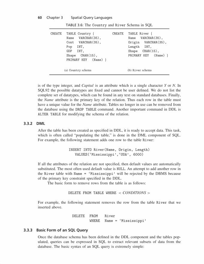
The creation of the relational schema and the addition and deletion of the tables arespecified in the DDL component of SQL. For example, the City schema introduced inSection 3.2 is defined below in SQL. The Country and River tables are defined inTable 3.6.

CREATE TABLE CITY {Name VARCHAR(35),

Country VARCHAR(35),

Pop INT,

Capital CHAR(1),

Shape CHAR(13),

PRIMARY KEY Name }

The CREATE TABLE statement is used to define the relations in a relationalschema. The name of the table is CITY. The table has four columns, and the name ofeach column and its corresponding datatype must be specified. The Name and Countryattributes must be ASCII character strings of less than thirty-five characters. Population


�

�

�

�

�

�

�

�


TABLE 3.6: The Country and River Schema in SQL

CREATE TABLE Country {Name VARCHAR(35),

Cont VARCHAR(35),

Pop INT,

GDP INT,

Shape CHAR(15),

PRIMARY KEY (Name) }

(a) Country schema

CREATE TABLE River {Name VARCHAR(35),

Origin VARCHAR(35),

Length INT,

Shape CHAR(15),

PRIMARY KEY (Name) }

(b) River schema

is of the type integer, and Capital is an attribute which is a single character Y or N. InSQL92 the possible datatypes are fixed and cannot be user defined. We do not list thecomplete set of datatypes, which can be found in any text on standard databases. Finally,the Name attribute is the primary key of the relation. Thus each row in the table musthave a unique value for the Name attribute. Tables no longer in use can be removed fromthe database using the DROP TABLE command. Another important command in DDL isALTER TABLE for modifying the schema of the relation.

3.3.2 DML

After the table has been created as specified in DDL, it is ready to accept data. This task,which is often called “populating the table,” is done in the DML component of SQL.For example, the following statement adds one row to the table River:

INSERT INTO River(Name, Origin, Length)

VALUES(‘Mississippi’,‘USA’, 6000)

If all the attributes of the relation are not specified, then default values are automaticallysubstituted. The most often used default value is NULL. An attempt to add another row inthe River table with Name = ‘Mississippi’ will be rejected by the DBMS becauseof the primary key constraint specified in the DDL.

The basic form to remove rows from the table is as follows:

DELETE FROM TABLE WHERE < CONDITIONS >

For example, the following statement removes the row from the table River that weinserted above.

DELETE FROM River

WHERE Name = ‘Mississippi’

3.3.3 Basic Form of an SQL Query

Once the database schema has been defined in the DDL component and the tables pop-ulated, queries can be expressed in SQL to extract relevant subsets of data from thedatabase. The basic syntax of an SQL query is extremely simple:


�

�

�

�

�

�

�

�


SELECT column-namesFROM relationsWHERE tuple-constraint

This form is equivalent to the RA expression consisting of π , σ , and ��. SQLSELECT statement has more clauses related to aggregation (e.g., GROUP BY, HAVING),ordering results (e.g., ORDER BY), and so forth. In addition, SQL allows the formulationof nested queries. We illustrate these with a set of examples.

3.3.4 Example Queries in SQL

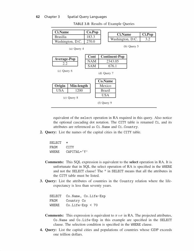
We now give examples of how to pose different types of queries in SQL. Our purpose isto give a flavor of the versatility and power of SELECT statement. All the tables queriedare from the WORLD example introduced in Section 3.1.1. The results of the differentqueries can be found in Tables 3.7 and 3.8.

1. Query: List all the cities and the country they belong to in the CITY table.

SELECT Ci.Name, Ci.Country

FROM CITY Ci

Comments: The SQL expression is equivalent to the project operation in RA.The WHERE clause is missing in the SQL expression because there is no

TABLE 3.7: Tables from the Select, Project, and Selectand Project Operations

Name Country Pop(millions) Capital ShapeHavana Cuba 2.1 Y Point

Washington, D.C. USA 3.2 Y PointBrasilia Brazil 1.5 Y PointOttawa Canada 0.8 Y Point

Mexico City Mexico 14.1 Y PointBuenos Aires Argentina 10.75 Y Point

(a) Query 2 Select

Name CountryHavana Cuba

Washington, D.C. USAMonterrey Mexico

Toronto CanadaBrasilia BrazilRosario ArgentinaOttawa Canada

Mexico City MexicoBuenos Aires Argentina

(b) Query 1 Project

Name Life-expMexico 69.36Brazil 65.60

(c) Query 3: Select andproject


�

�

�

�

�

�

�

�


TABLE 3.8: Results of Example Queries

Ci.Name Co.PopBrasilia 183.3Washington, D.C. 270.0

(a) Query 4

Ci.Name Ci.PopWashington, D.C. 3.2

(b) Query 5

Average-Pop2.2

(c) Query 6

Cont Continent-PopNAM 2343.05SAM 676.1

(d) Query 7

Origin Min-lengthUSA 1200

(e) Query 8

Co.NameMexicoBrazilUSA

(f) Query 9

equivalent of the select operation in RA required in this query. Also noticethe optional cascading dot notation. The CITY table is renamed Ci, and itsattributes are referenced as Ci.Name and Ci.Country.

2. Query: List the names of the capital cities in the CITY table.

SELECT *

FROM CITY

WHERE CAPITAL=‘Y’

Comments: This SQL expression is equivalent to the select operation in RA. It isunfortunate that in SQL the select operation of RA is specified in the WHERE

and not the SELECT clause! The * in SELECT means that all the attributes inthe CITY table must be listed.

3. Query: List the attributes of countries in the Country relation where the life-expectancy is less than seventy years.

SELECT Co.Name, Co.Life-Exp

FROM Country Co

WHERE Co.Life-Exp < 70

Comments: This expression is equivalent to π ◦σ in RA. The projected attributes,Co.Name and Co.Life-Exp in this example are specified in the SELECT

clause. The selection condition is specified in the WHERE clause.

4. Query: List the capital cities and populations of countries whose GDP exceedsone trillion dollars.


�

�

�

�

�

�

�

�


SELECT Ci.Name, Co.Pop

FROM City Ci, Country Co

WHERE Ci.Country = Co.Name AND

Co.GDP > 1000.0 AND

Ci.Capital= ‘Y’

Comments: This is an implicit way of expressing the join operation. SQL2 andSQL3 also support an explicit JOIN operation. In this case the two tablesCity and Country are matched on their common attributes Ci.country andCo.name. Furthermore, two selection conditions are specified separately onthe City and Country table. Notice how the cascading dot notation alleviatedthe potential confusion that might have arisen as a result of the attribute namesin the two relations.

5. Query: What is the name and population of the capital city in the country wherethe St. Lawrence River originates?

SELECT Ci.Name, Ci.Pop

FROM City Ci, Country Co, River R

WHERE R.Origin = Co.Name AND

Co.Name = Ci.Country AND

R.Name = ‘St. Lawrence’ AND

Ci.Capital= ‘Y’

Comments: This query involves a join among three tables. The River and Country

tables are joined on the attributes Origin and Name. The Country and theCity tables are joined on the attributes Name and Country. There are twoselection conditions on the River and the City tables respectively.

6. Query: What is the average population of the noncapital cities listed in the City

table?

SELECT AVG(Ci.Pop)

FROM City Ci

WHERE Ci.Capital= ‘N’

Comments: The AVG (Average) is an example of an aggregate operation. Theseoperations are not available in RA. Besides AVG, other aggregate operationsare COUNT, MAX, MIN, and SUM. The aggregate operations expand the func-tionality of SQL because they allow computations to be performed on theretrieved data.

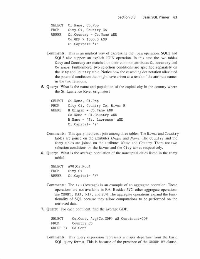
7. Query: For each continent, find the average GDP.

SELECT Co.Cont, Avg(Co.GDP) AS Continent-GDP

FROM Country Co

GROUP BY Co.Cont

Comments: This query expression represents a major departure from the basicSQL query format. This is because of the presence of the GROUP BY clause.


�

�

�

�

�

�

�

�


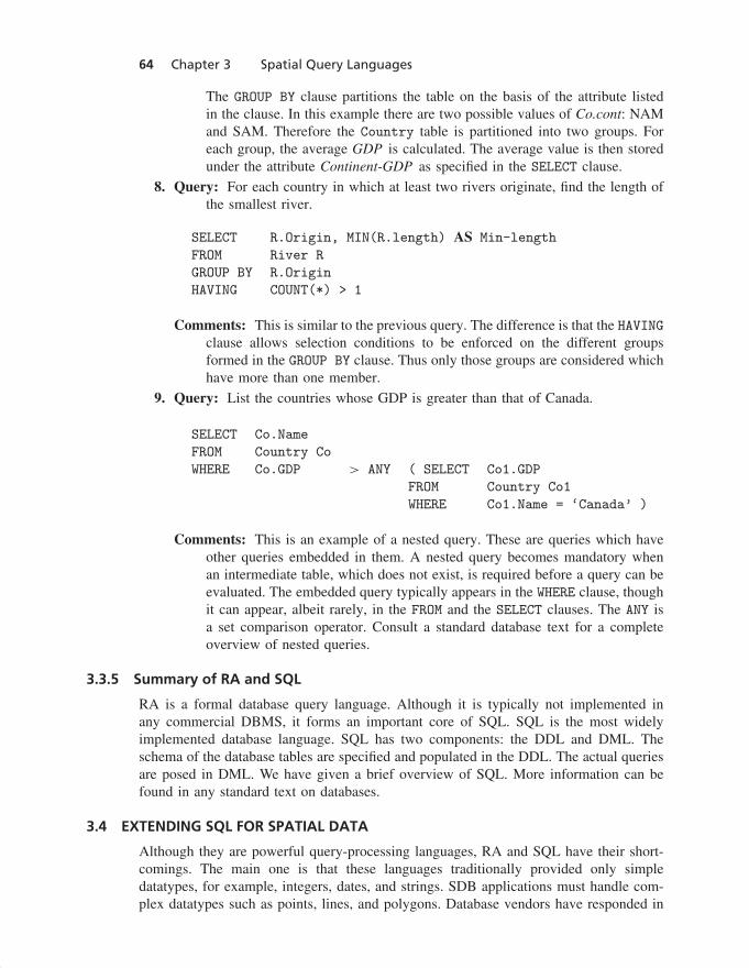
The GROUP BY clause partitions the table on the basis of the attribute listedin the clause. In this example there are two possible values of Co.cont: NAMand SAM. Therefore the Country table is partitioned into two groups. Foreach group, the average GDP is calculated. The average value is then storedunder the attribute Continent-GDP as specified in the SELECT clause.

8. Query: For each country in which at least two rivers originate, find the length ofthe smallest river.

SELECT R.Origin, MIN(R.length) AS Min-length

FROM River R

GROUP BY R.Origin

HAVING COUNT(*) > 1

Comments: This is similar to the previous query. The difference is that the HAVINGclause allows selection conditions to be enforced on the different groupsformed in the GROUP BY clause. Thus only those groups are considered whichhave more than one member.

9. Query: List the countries whose GDP is greater than that of Canada.

SELECT Co.Name

FROM Country Co

WHERE Co.GDP > ANY ( SELECT Co1.GDP

FROM Country Co1

WHERE Co1.Name = ‘Canada’ )

Comments: This is an example of a nested query. These are queries which haveother queries embedded in them. A nested query becomes mandatory whenan intermediate table, which does not exist, is required before a query can beevaluated. The embedded query typically appears in the WHERE clause, thoughit can appear, albeit rarely, in the FROM and the SELECT clauses. The ANY isa set comparison operator. Consult a standard database text for a completeoverview of nested queries.

3.3.5 Summary of RA and SQL

RA is a formal database query language. Although it is typically not implemented inany commercial DBMS, it forms an important core of SQL. SQL is the most widelyimplemented database language. SQL has two components: the DDL and DML. Theschema of the database tables are specified and populated in the DDL. The actual queriesare posed in DML. We have given a brief overview of SQL. More information can befound in any standard text on databases.

3.4 EXTENDING SQL FOR SPATIAL DATA

Although they are powerful query-processing languages, RA and SQL have their short-comings. The main one is that these languages traditionally provided only simpledatatypes, for example, integers, dates, and strings. SDB applications must handle com-plex datatypes such as points, lines, and polygons. Database vendors have responded in


�

�

�

�

�

�

�

�

Section 3.4 Extending SQL for Spatial Data 65

two ways: They have either used blobs to store spatial information, or they have createda hybrid system in which spatial attributes are stored in operating-system files via a GIS.SQL cannot process data stored as blobs, and it is the responsibility of the applicationtechniques to handle data in blob form [Stonebraker and Moore, 1997]. This solution isneither efficient nor aesthetic because the data depends on the host-language applicationcode. In a hybrid system, spatial attributes are stored in a separate operating-system fileand thus are unable to take advantage of traditional database services such as querylanguage, concurrency control, and indexing support.

Object-oriented systems have had a major influence on expanding the capabilities ofDBMS to support spatial (complex) objects. The program to extend a relational databasewith object-oriented features falls under the general framework of OR-DBMS. The keyfeature of OR-DBMS is that it supports a version of SQL, SQL3/SQL99, which supportsthe notion of user-defined types (as in Java or C++). Our goal is to study SQL3/SQL99enough so that we can use it as a tool to manipulate and retrieve spatial data.

The principle demand of spatial SQL is to provide a higher abstraction of spatialdata by incorporating concepts closer to our perception of space [Egenhofer, 1994]. Thisis accomplished by incorporating the object-oriented concept of user-defined ADTs. AnADT is a user-defined type and its associated functions. For example, if we have landparcels stored as polygons in a database, then a useful ADT may be a combination ofthe type polygon and some associated function (method), say, adjacent. The adjacent

function may be applied to land parcels to determine if they share a common bound-ary. The term abstract is used because the end user need not know the implementationdetails of the associated functions. All end users need to know is the interface, that is,the available functions and the data types for the input parameters and output results.

3.4.1 The OGIS Standard for Extending SQL

The OGIS consortium was formed by major software vendors to formulate an industrywide standard related to GIS interoperability. The OGIS spatial data model can be em-bedded in a variety of programming languages, for example, C, Java, SQL, and so on.We focus on SQL embedding in this section.

The OGIS is based on a geometry data model shown in Figure 2.2. Recall thatthe data model consists of a base-class, GEOMETRY, which is noninstantiable (i.e., objectscannot be defined as instances of GEOMETRY), but specifies a spatial reference systemapplicable to all its subclasses. The four major subclasses derived from the GEOMETRY

superclass are Point, Curve Surface and GeometryCollection. Associated witheach class is a set of operations that acts on instances of the classes. A subset of importantoperations and their definitions are listed in Table 3.9.

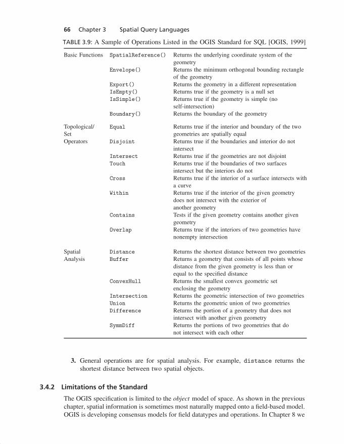
The operations specified in the OGIS standard fall into three categories:

1. Basic operations apply to all geometry datatypes. For example, SpatialReferencereturns the underlying coordinate system where the geometry of the object was de-fined. Examples of common reference systems include the well-known latitude andlongitude system and the often-used Universal Traversal Mercator (UTM).

2. Operations test for topological relationships between spatial objects. For example,overlap tests whether the interior (see Chapter 2) of two objects has a nonemptyset intersection.


�

�

�

�

�

�

�

�


TABLE 3.9: A Sample of Operations Listed in the OGIS Standard for SQL [OGIS, 1999]

Basic Functions SpatialReference() Returns the underlying coordinate system of thegeometry

Envelope() Returns the minimum orthogonal bounding rectangleof the geometry

Export() Returns the geometry in a different representationIsEmpty() Returns true if the geometry is a null setIsSimple() Returns true if the geometry is simple (no

self-intersection)Boundary() Returns the boundary of the geometry

Topological/ Equal Returns true if the interior and boundary of the twoSet geometries are spatially equalOperators Disjoint Returns true if the boundaries and interior do not

intersectIntersect Returns true if the geometries are not disjointTouch Returns true if the boundaries of two surfaces

intersect but the interiors do notCross Returns true if the interior of a surface intersects with

a curveWithin Returns true if the interior of the given geometry

does not intersect with the exterior ofanother geometry

Contains Tests if the given geometry contains another givengeometry

Overlap Returns true if the interiors of two geometries havenonempty intersection

Spatial Distance Returns the shortest distance between two geometriesAnalysis Buffer Returns a geometry that consists of all points whose

distance from the given geometry is less than orequal to the specified distance

ConvexHull Returns the smallest convex geometric setenclosing the geometry

Intersection Returns the geometric intersection of two geometriesUnion Returns the geometric union of two geometriesDifference Returns the portion of a geometry that does not

intersect with another given geometrySymmDiff Returns the portions of two geometries that do

not intersect with each other

3. General operations are for spatial analysis. For example, distance returns theshortest distance between two spatial objects.

3.4.2 Limitations of the Standard

The OGIS specification is limited to the object model of space. As shown in the previouschapter, spatial information is sometimes most naturally mapped onto a field-based model.OGIS is developing consensus models for field datatypes and operations. In Chapter 8 we


�

�

�

�

�

�

�

�

Section 3.5 Example Queries that Emphasize Spatial Aspects 67

introduce some relevant operations for the field-based model which may be incorporatedinto a future OGIS standard.

Even within the object model, the OGIS operations are limited for simpleSELECT-PROJECT-JOIN queries. Support for spatial aggregate queries with the GROUP

BY and HAVING clauses does pose problems (see Exercise 4). Finally, the focus inthe OGIS standard is exclusively on basic topological and metric spatial relationships.Support for a whole class of metric operations, namely, those based on the directionpredicate (e.g., north, south, left, front), is missing. It also does not support dynamic,shape-based, and visibility-based operations discussed in Section 2.1.5.

3.5 EXAMPLE QUERIES THAT EMPHASIZE SPATIAL ASPECTS

Using the OGIS datatypes and operations, we formulate SQL queries in the World

database which highlight the spatial relationships between the three entities: Country,City, and River. We first redefine the relational schema, assuming that the OGISdatatypes and operations are available in SQL. Revised schema is shown in Table 3.10.

1. Query: Find the names of all countries which are neighbors of the United States(USA) in the Country table.

SELECT C1.Name AS "Neighbors of USA"

FROM Country C1, Country C2

WHERE Touch(C1.Shape, C2.Shape) = 1 AND

C2.Name = ‘USA’

Comments: The Touch predicate checks if any two geometric objects are adja-cent to each other without overlapping. It is a useful operation to determineneighboring geometric objects. The Touch operation is one of the eight topo-logical predicates specified in the OGIS standard. One of the nice properties

TABLE 3.10: Basic Tables

CREATE TABLE Country(

Name varchar(30),

Cont varchar(30),

Pop Integer,

GDP Number,

Shape Polygon);

(a)

CREATE TABLE River(

Name varchar(30),

Origin varchar(30),

Length Number,

Shape LineString);

(b)

CREATE TABLE City (

Name varchar(30),

Country varchar(30),

Pop integer,

Shape Point );

(c)


�

�

�

�

�

�

�

�


of topological operations is that they are invariant under many geometrictransformations. In particular the choice of the coordinate system for theWorld database will not affect the results of topological operations.Topological operations apply to many different combinations of geometrictypes. Therefore, in an ideal situation these operations should be defined inan “overloaded” fashion. Unfortunately, many object-relational DBMSs donot support object-oriented notions of class inheritance and operation over-loading. Thus, for all practical purposes these operations may be definedindividually for each combination of applicable geometric types.

2. Query: For all the rivers listed in the River table, find the countries throughwhich they pass.

SELECT R.Name C.Name

FROM River R, Country C

WHERE Cross(R.Shape, C.Shape) = 1

Comments: The Cross is also a topological predicate. It is most often used tocheck for the intersection between a LineString and Polygon objects, asin this example, or a pair of LineString objects.

3. Query: Which city listed in the City table is closest to each river listed in theRiver table?

SELECT C1.Name, R1.Name

FROM City C1, River R1

WHERE Distance (C1.Shape, R1.Shape) <

ALL (SELECT Distance(C2.Shape, R1.Shape)

FROM City C2

WHERE C1.Name <> C2.Name

)

Comments: The Distance is a real-valued binary operation. It is being usedonce in the WHERE clause and again in the SELECT clause of the subquery.The Distance function is defined for any combination of geometric objects.

4. Query: The St. Lawrence River can supply water to cities that are within 300 km.List the cities that can use water from the St. Lawrence.

SELECT Ci.Name

FROM City Ci, River R

WHERE Overlap(Ci.Shape, Buffer(R.Shape,300)) = 1 AND

R.Name = ‘St. Lawrence’

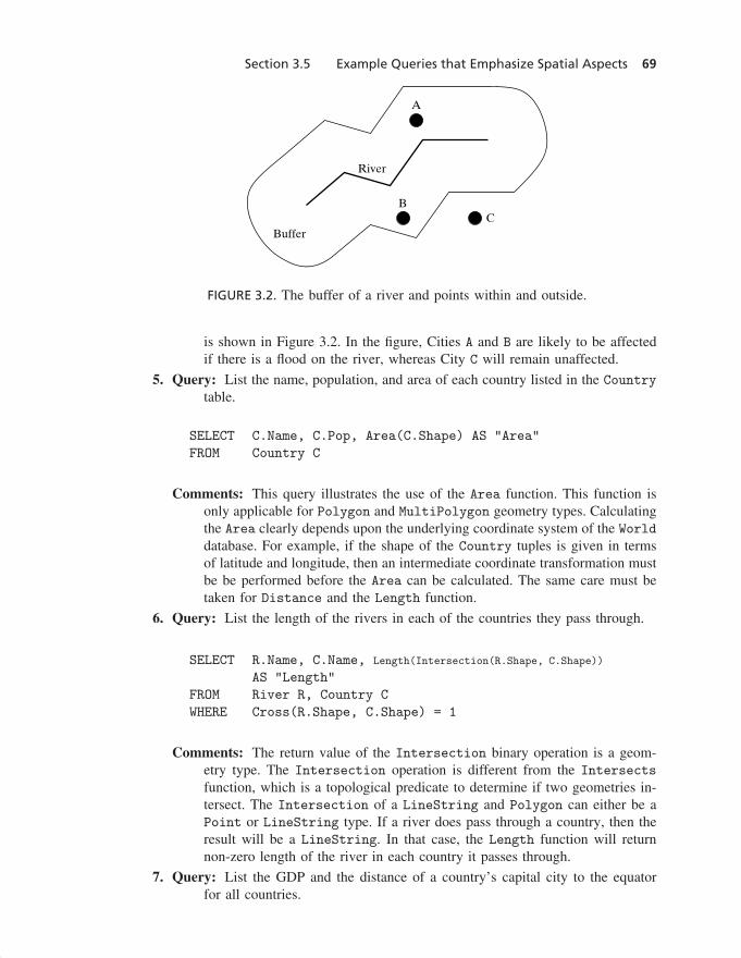
Comments: The Buffer of a geometric object is a geometric region centered atthe object whose size is determined by a parameter in the Buffer operation.In the example the query dictates the size of the buffer region. The bufferoperation is used in many GIS applications, including floodplain managementand urban and rural zoning laws. A graphical depiction of the buffer operation


�

�

�

�

�

�

�

�

Section 3.5 Example Queries that Emphasize Spatial Aspects 69

River

Buffer

A

BC

FIGURE 3.2. The buffer of a river and points within and outside.

is shown in Figure 3.2. In the figure, Cities A and B are likely to be affectedif there is a flood on the river, whereas City C will remain unaffected.

5. Query: List the name, population, and area of each country listed in the Country

table.

SELECT C.Name, C.Pop, Area(C.Shape) AS "Area"

FROM Country C

Comments: This query illustrates the use of the Area function. This function isonly applicable for Polygon and MultiPolygon geometry types. Calculatingthe Area clearly depends upon the underlying coordinate system of the Worlddatabase. For example, if the shape of the Country tuples is given in termsof latitude and longitude, then an intermediate coordinate transformation mustbe be performed before the Area can be calculated. The same care must betaken for Distance and the Length function.

6. Query: List the length of the rivers in each of the countries they pass through.

SELECT R.Name, C.Name, Length(Intersection(R.Shape, C.Shape))

AS "Length"

FROM River R, Country C

WHERE Cross(R.Shape, C.Shape) = 1

Comments: The return value of the Intersection binary operation is a geom-etry type. The Intersection operation is different from the Intersects

function, which is a topological predicate to determine if two geometries in-tersect. The Intersection of a LineString and Polygon can either be aPoint or LineString type. If a river does pass through a country, then theresult will be a LineString. In that case, the Length function will returnnon-zero length of the river in each country it passes through.

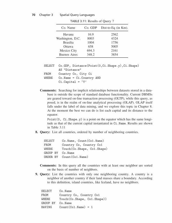
7. Query: List the GDP and the distance of a country’s capital city to the equatorfor all countries.


�

�

�

�

�

�

�

�


TABLE 3.11: Results of Query 7

Co. Name Co. GDP Dist-to-Eq (in Km).

Havana 16.9 2562Washington, D.C. 8003 4324

Brasilia 1004 1756Ottawa 658 5005

Mexico City 694.3 2161Buenos Aires 348.2 3854

SELECT Co.GDP, Distance(Point(0,Ci.Shape.y),Ci.Shape)

AS "Distance"

FROM Country Co, City Ci

WHERE Co.Name = Ci.Country AND

Ci.Capital = ‘Y’

Comments: Searching for implicit relationships between datasets stored in a data-base is outside the scope of standard database functionality. Current DBMSsare geared toward on-line transaction processing (OLTP), while this query, asposed, is in the realm of on-line analytical processing (OLAP). OLAP itselffalls under the label of data mining, and we explore this topic in Chapter 8.At the moment the best we can do is list each capital and its distance to theequator.

Point(0, Ci.Shape.y) is a point on the equator which has the same longi-tude as that of the current capital instantiated in Ci.Name. Results are shownin Table 3.11

8. Query: List all countries, ordered by number of neighboring countries.

SELECT Co.Name, Count(Co1.Name)

FROM Country Co, Country Co1

WHERE Touch(Co.Shape, Co1.Shape)

GROUP BY Co.Name

ORDER BY Count(Co1.Name)

Comments: In this query all the countries with at least one neighbor are sortedon the basis of number of neighbors.

9. Query: List the countries with only one neighboring country. A country is aneighbor of another country if their land masses share a boundary. Accordingto this definition, island countries, like Iceland, have no neighbors.

SELECT Co.Name


WHERE Touch(Co.Shape, Co1.Shape))

GROUP BY Co.Name

HAVING Count(Co1.Name) = 1


�

�

�

�

�

�

�

�

Section 3.6 Trends: Object-Relational SQL 71

SELECT Co.Name

FROM Country Co

WHERE Co.Name IN

(SELECT Co.Name



GROUP BY Co.Name

HAVING Count(*) = 1)

Comments: Here we have a nested query in the FROM clause. The result of thequery within the FROM clause is a table consisting of pairs of countries whichare neighbors. The GROUP BY clause partitions the new table on the basis ofthe names of the countries. Finally the HAVING clause forces the selection tobe paired to those countries that have only one neighbor. The HAVING clauseplays a role similar to the WHERE clause with the exception that it must includesuch aggregate functions as count, sum, max, and min.

10. Query: Which country has the maximum number of neighbors?

CREATE VIEW Neighbor AS

SELECT Co.Name, Count(Co1.Name) AS num neighbors



GROUP BY Co.Name

SELECT Co.Name, num neighbors

FROM Neighbor

WHERE num neighbor = (SELECT Max(num neighbors)

FROM Neighbor)

Comments: This query demonstrates the use of views in simplifying complexqueries. First query (view) computes the number of neighbors for each coun-try. This view creates a virtual table which can be used as a normal tablein subsequent queries. The second query selects the country with the largestnumber of neighbors from the Neighbor view.

3.6 TRENDS: OBJECT-RELATIONAL SQL

The OGIS standard specifies the datatypes and their associated operations which areconsidered essential for spatial applications such as GIS. For example, for the Point

datatype an important operation is Distance, which computes the distance between twopoints. The length operation is not a semantically correct operation on a Point datatype.This is similar to the argument that the concatenation operation makes more sense forCharacter datatype than for, say, the Integer type.

In relational databases the set of datatypes is fixed. In object-relational and object-oriented databases, this limitation has been relaxed, and there is built in support foruser-defined datatypes. Even though this feature is clearly an advantage, especiallywhen dealing with nontraditional database applications such as GIS, the burden of


�

�

�

�

�

�

�

�


constructing syntactically and semantically correct datatypes is now on the databaseapplication developer. To share some of the burden, commercial database vendors haveintroduced application-specific “packages” which provide a seamless interface to thedatabase user. For example, Oracle markets a GIS specific package called the Spatial

Data Cartridge.SQL3/SQL99, the proposed SQL standard for OR-DBMS allows user-defined

datatypes within the overall framework of a relational database. Two features of theSQL3 standard that may be beneficial for defining user-defined spatial datatypes aredescribed below.

3.6.1 A Glance at SQL3

The SQL3/SQL99 proposes two major extensions to SQL2/SQL92, the current acceptedSQL draft.

1. ADT: An ADT can be defined using a CREATE TYPE statement. Like classes inobject-oriented technology, an ADT consists of attributes and member functions toaccess the values of the attributes. Member functions can potentially modify thevalue of the attributes in the datatype and thus can also change the database state.

An ADT can appear as a column type in a relational schema. To access the valuethat the ADT encapsulates, a member function specified in the CREATE TYPE mustbe used. For example, the following script creates a type Point with the definitionof one member function Distance:

CREATE TYPE Point (

x NUMBER,

y NUMBER,

FUNCTION Distance(:u Point,:v Point)

RETURNS NUMBER

);

The colons before u and v signify that these are local variables.

2. Row Type: A row type is a type for a relation. A row type specifies the schemaof a relation. For example the following statement creates a row type Point.

CREATE ROW TYPE Point (

x NUMBER,

y NUMBER );

We can now create a table that instantiates the row type. For example:

CREATE TABLE Pointtable of TYPE Point;

In this text we emphasize the use of ADT instead of row type. This is because the ADTas a column type naturally harmonizes the definition of an OR-DBMS as an extendedrelational database.


�

�

�

�

�

�

�

�

Section 3.6 Trends: Object-Relational SQL 73

3.6.2 Object-Relational Schema

Oracle8 is an OR-DBMS introduced by the Oracle Corporation. Similar products areavailable from other database companies, for example, IBM. OR-DBMS implements apart of the SQL3 Standard. The ADT is called the “object type” in this system.

Below we describe how the three basic spatial datatypes: Point, LineString,

and Polygon are constructed in Oracle8.

CREATE TYPE Point AS OBJECT (

x NUMBER,

y NUMBER,

MEMBER FUNCTION Distance(P2 IN Point) RETURN NUMBER,

PRAGMA RESTRICT REFERENCES(Distance, WNDS));

The Point type has two attributes, x and y, and one member function, Distance.PRAGMA alludes to the fact that the Distance function will not modify the state of thedatabase: WNDS (Write No Database State). Of course in the OGIS standard many otheroperations related to the Point type are specified, but for simplicity we have shown onlyone. After its creation the Point type can be used in a relation as an attribute type. Forexample, the schema of the relation City can be defined as follows:

CREATE TABLE City (

Name varchar(30),

Country varchar(35),

Pop int,

Capital char(1),

Shape Point );

Once the relation schema has been defined, the table can be populated in the usualway. For example, the following statement adds information related to Brasilia, thecapital of Brazil, into the database

INSERT INTO CITY(‘̄Brasilia’, ‘Brazil’, 1.5, ‘Y’,

Point(-55.4,-23.2));

The construction of the LineString datatype is slightly more involved than thatof the Point type. We begin by creating an intermediate type, LineType:

CREATE TYPE LineType AS VARRAY(500) OF Point;

Thus LineType is a variable array of Point datatype with a maximum length of 500.Type specific member functions cannot be defined if the type is defined as a Varray.Therefore we create another type LineString

CREATE TYPE LineString AS OBJECT (

Num of Points INT,

Geometry LineType,

MEMBER FUNCTION Length(SELF IN) RETURN NUMBER,

PRAGMA RESTRICT REFERENCES(Length, WNDS));


�

�

�

�

�

�

�

�


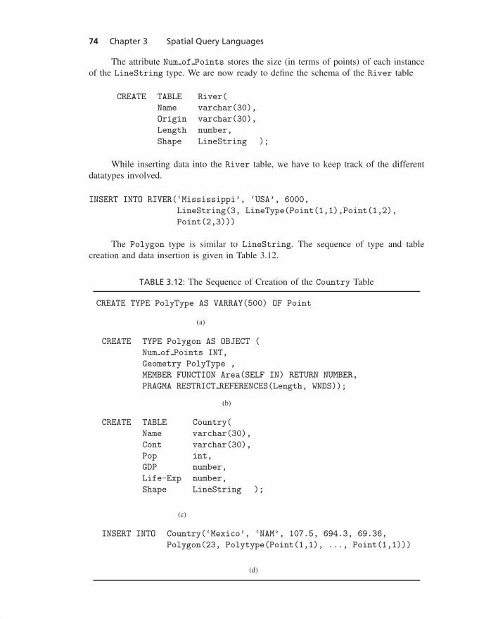
The attribute Num of Points stores the size (in terms of points) of each instanceof the LineString type. We are now ready to define the schema of the River table

CREATE TABLE River(

Name varchar(30),

Origin varchar(30),

Length number,

Shape LineString );

While inserting data into the River table, we have to keep track of the differentdatatypes involved.

INSERT INTO RIVER(‘Mississippi’, ‘USA’, 6000,

LineString(3, LineType(Point(1,1),Point(1,2),

Point(2,3)))

The Polygon type is similar to LineString. The sequence of type and tablecreation and data insertion is given in Table 3.12.

TABLE 3.12: The Sequence of Creation of the Country Table

CREATE TYPE PolyType AS VARRAY(500) OF Point

(a)

CREATE TYPE Polygon AS OBJECT (

Num of Points INT,

Geometry PolyType ,

MEMBER FUNCTION Area(SELF IN) RETURN NUMBER,

PRAGMA RESTRICT REFERENCES(Length, WNDS));

(b)

CREATE TABLE Country(

Name varchar(30),

Cont varchar(30),

Pop int,

GDP number,

Life-Exp number,

Shape LineString );

(c)

INSERT INTO Country(‘Mexico’, ‘NAM’, 107.5, 694.3, 69.36,

Polygon(23, Polytype(Point(1,1), ..., Point(1,1)))

(d)


�

�

�

�

�

�

�

�

Section 3.7 Summary 75

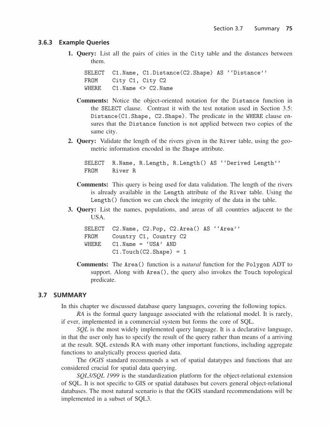
3.6.3 Example Queries

1. Query: List all the pairs of cities in the City table and the distances betweenthem.

SELECT C1.Name, C1.Distance(C2.Shape) AS ‘‘Distance’’

FROM City C1, City C2

WHERE C1.Name <> C2.Name

Comments: Notice the object-oriented notation for the Distance function inthe SELECT clause. Contrast it with the test notation used in Section 3.5:Distance(C1.Shape, C2.Shape). The predicate in the WHERE clause en-sures that the Distance function is not applied between two copies of thesame city.

2. Query: Validate the length of the rivers given in the River table, using the geo-metric information encoded in the Shape attribute.

SELECT R.Name, R.Length, R.Length() AS ‘‘Derived Length’’

FROM River R

Comments: This query is being used for data validation. The length of the riversis already available in the Length attribute of the River table. Using theLength() function we can check the integrity of the data in the table.

3. Query: List the names, populations, and areas of all countries adjacent to theUSA.

SELECT C2.Name, C2.Pop, C2.Area() AS ‘‘Area’’

FROM Country C1, Country C2

WHERE C1.Name = ‘USA’ AND

C1.Touch(C2.Shape) = 1

Comments: The Area() function is a natural function for the Polygon ADT tosupport. Along with Area(), the query also invokes the Touch topologicalpredicate.

3.7 SUMMARY

In this chapter we discussed database query languages, covering the following topics.RA is the formal query language associated with the relational model. It is rarely,

if ever, implemented in a commercial system but forms the core of SQL.SQL is the most widely implemented query language. It is a declarative language,

in that the user only has to specify the result of the query rather than means of a arrivingat the result. SQL extends RA with many other important functions, including aggregatefunctions to analytically process queried data.

The OGIS standard recommends a set of spatial datatypes and functions that areconsidered crucial for spatial data querying.

SQL3/SQL 1999 is the standardization platform for the object-relational extensionof SQL. It is not specific to GIS or spatial databases but covers general object-relationaldatabases. The most natural scenario is that the OGIS standard recommendations will beimplemented in a subset of SQL3.


�

�

�

�

�

�

�

�


BIBLIOGRAPHIC NOTES

3.1, 3.2, 3.3 A complete exposition of relational algebra and SQL can be found in any introductorytext in databases, including [Elmasri and Navathe, 2000; Ramakrishnan, 1998; Ullmanand Widom, 1999].

3.4, 3.5 Extensions of SQL for spatial applications are explored in [Egenhofer, 1994]. TheOGIS document [OpenGIS, 1998] is an attempt to harmonize the different spatialextensions of SQL. For an example of query languages in supporting spatial dataanalysis, see [Lin and Huang, 2001].

3.6 SQL 1999/SQL3 is the adopted standard for the object-relational extension of SQL.Subsets of the standard have already been implemented in commercial products,including Oracle’s Oracle8 and IBM’s DB2.

EXERCISES

For all queries in Exercises 1 and 2 refer to Table 3.1.

1. Express the following queries in relational algebra.(a) Find all countries whose GDP is greater than $500 billion but less than $1 trillion.(b) List the life expectancy in countries that have rivers originating in them.(c) Find all cities that are either in South America or whose population is less than

two million.(d) List all cities which are not in South America.

2. Express in SQL the queries listed in Exercise 1.3. Express the following queries in SQL.

(a) Count the number of countries whose population is less than 100 million.(b) Find the country in North America with the smallest GDP. Do not use the MIN

function. Hint: nested query.(c) List all countries that are in North America or whose capital cities have a popu-

lation of less than 5 million.(d) Find the country with the second highest GDP.

4. The Reclassify (see Section 2.1.5) is an aggregate function that combines spatialgeometries on the basis of nonspatial attributes. It creates new objects from the existingones, generally by removing the internal boundaries of the adjacent polygons whosechosen attribute is same. Can we express the Reclassify operation using OGISoperations and SQL92 with spatial datatypes? Explain.

5. Discuss the geometry data model of Figure 2.2. Given that on a “world” scale, citiesare represented as point datatypes, what datatype should be used to represent thecountries of the world. Note: Singapore, the Vatican, and Monaco are countries. Whatare the implementation implications for the spatial functions recommended by theOGIS standard.

6. [Egenhofer, 1994] proposes a list of requirements for extending SQL for spatial appli-cations. The requirements are shown below. Which of these the recommendations havebeen accepted in the OGIS SQL standard? Discuss possible reasons for postponingthe others.

7. The OGIS standard includes a set of topological spatial predicates. How should thestandard be extended to include directional predicates such as East, North,North-East, and so forth. Note that the directional predicates may be fuzzy: “Wheredoes North-East end and East begin?”

8. This exercise surveys the dimension-extended nine-intersection model: DE-9IM. TheDE-9IM extends Egenhofer’s nine-intersection model introduced in Chapter 2. The


�

�

�

�

�

�

�

�

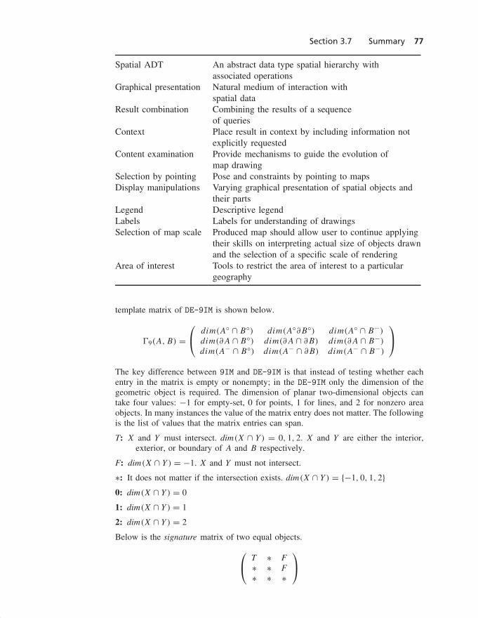
Section 3.7 Summary 77

Spatial ADT An abstract data type spatial hierarchy withassociated operations

Graphical presentation Natural medium of interaction withspatial data

Result combination Combining the results of a sequenceof queries

Context Place result in context by including information notexplicitly requested

Content examination Provide mechanisms to guide the evolution ofmap drawing

Selection by pointing Pose and constraints by pointing to mapsDisplay manipulations Varying graphical presentation of spatial objects and

their partsLegend Descriptive legendLabels Labels for understanding of drawingsSelection of map scale Produced map should allow user to continue applying

their skills on interpreting actual size of objects drawnand the selection of a specific scale of rendering

Area of interest Tools to restrict the area of interest to a particulargeography

template matrix of DE-9IM is shown below.

�9(A,B) =

dim(A◦ ∩ B◦) dim(A◦∂B◦) dim(A◦ ∩ B−)dim(∂A ∩ B◦) dim(∂A ∩ ∂B) dim(∂A ∩ B−)dim(A− ∩ B◦) dim(A− ∩ ∂B) dim(A− ∩ B−)

The key difference between 9IM and DE-9IM is that instead of testing whether eachentry in the matrix is empty or nonempty; in the DE-9IM only the dimension of thegeometric object is required. The dimension of planar two-dimensional objects cantake four values: −1 for empty-set, 0 for points, 1 for lines, and 2 for nonzero areaobjects. In many instances the value of the matrix entry does not matter. The followingis the list of values that the matrix entries can span.

T: X and Y must intersect. dim(X ∩ Y ) = 0, 1, 2. X and Y are either the interior,exterior, or boundary of A and B respectively.

F: dim(X ∩ Y ) = −1. X and Y must not intersect.

∗: It does not matter if the intersection exists. dim(X ∩ Y ) = {−1, 0, 1, 2}0: dim(X ∩ Y ) = 0

1: dim(X ∩ Y ) = 1

2: dim(X ∩ Y ) = 2

Below is the signature matrix of two equal objects.

T ∗ F

∗ ∗ F

∗ ∗ ∗


�

�

�

�

�

�

�

�


(a) What is the signature matrix (matrices) of the touch and cross topologicaloperations? Note that the signature matrix depends on the combination of thedatatypes. The signature matrix of a point/point combination is different fromthat of a multipolygon/multipolygon combination.

(b) What operation (and combination of datatypes) does the following signature ma-trix represent?

1 ∗ T

∗ ∗ F

T ∗ ∗

(c) Consider the sample figures shown Figure 3.3. What are signature matrices in9IM and DE-9IM. Is DE-9IM superior to 9IM? Discuss.

9. Express the following queries in SQL, using the OGIS extended datatype and functions.(a) List all cities in the City table which are within five thousand miles of Wash-

ington, D.C.(b) What is the length of Rio Paranas in Argentina and Brazil?(c) Do Argentina and Brazil share a border?(d) List the countries that lie completely south of the equator.

10. Given the schema:

RIVER(NAME:char, FLOOD-PLAIN:polygon, GEOMETRY:linstring)ROAD(ID:char, NAME:char, TYPE:char, GEOMETRY:linstring)

FOREST(NAME:char, GEOMETRY:polygon)LAND-PARCELS(ID:integer, GEOMETRY:polygon, county:char)

Transform the following queries into SQL using the OGIS specified datatypes andoperations.(a) Name all the rivers that cross Itasca State Forest.(b) Name all the tar roads that intersect Francis Forest.(c) All roads with stretches within the floodplain of the river Montana are susceptible

to flooding. Identify all these roads.(d) No urban development is allowed within two miles of the Red River and five

miles of the Big Tree State Park. Identify the landparcels and the county they arein that cannot be developed.

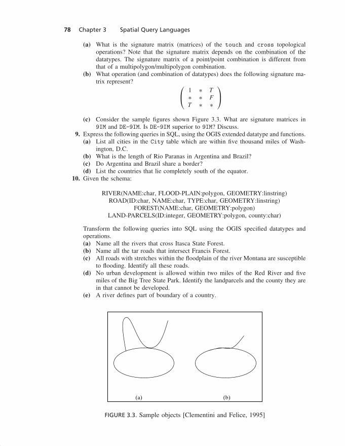
(e) A river defines part of boundary of a country.

(b)(a)

FIGURE 3.3. Sample objects [Clementini and Felice, 1995]


�

�

�

�

�

�

�

�

Section 3.8 Appendix: State Park Database 79

11. Study the compiler tools such as YACC (Yet Another Compiler Compiler). Develop asyntax scheme to generate SQL3 data definition statements from an Entity RelationshipDiagram (ERD) annotated with pictograms.

12. How would one model the following spatial relationships using 9-intersection modelor OGIS topological operations?(a) A river (LineString) originates in a country (Polygon)(b) A country (e.g., Vatican city) is completely surrounded by another (e.g., Italy)

country(c) A river (e.g., Missouri) falls into another (e.g., Mississippi) river(d) Forest stands partition a forest

13. Review the example RA queries provided for state park database in Appendix. WriteSQL expressions for each RA query.

14. Redraw the ER diagram provided in Figure 3.4 using pictograms. How will one rep-resent Fishing-Opener and Distance attributes in the new ER diagram. Generate tablesby translating the resulting ER diagram using SQL3/OGIS constructs.

15. Consider the table-designs in Figure 1.3 and 1.4. Describe SQL queries to computespatial properties (e.g. area, perimeter) of census blocks using each representation.Which representation lead to simple queries?

16. Revisit the Java program in Section 2.1.6. Design Java programs to carry out thespatial queries listed in Section 3.6.3. Compare and contrast querying spatial datasetusing Java with querying using SQL3/OGIS.

17. Define user defined data types for geometry aggregation data types in OGIS usingSQL3.

18. Revisit relational schema for state park example in Section 2.2.3. Outline SQL DMLstatements to create relevant tables using OGIS spatial data type.

19. Consider shape-based queries, for example, list countries shaped like ladies boot or listsquarish census blocks. Propose extensions to SQL3/OGIS to support such queries.

20. Consider visibility-based queries, for example, list objects visible (not occluded) froma vista-point and viewer orientation. Propose a set of data types and operations forextending SQL3/OGIS to support such queries.

3.8 APPENDIX: STATE PARK DATABASE

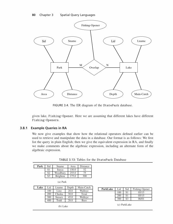
The State Park database consists of two entities: Park and Lake. The attributes ofthese two entities and their relationships are shown in Figure 3.4. The ER diagram ismapped into the relational schema shown below. The entities and their relationships arematerialized in Table 3.13.

StatePark(Sid: integer, Sname: string, Area: float, Distance: float)

Lake(Lid: integer, Lname: string, Depth: float, Main-Catch: string)

ParkLake(Lid: integer, Sid: integer, Fishing-Opener: date)

The above schema represents three entities: StatePark, Lake, and ParkLake.StatePark represents all the state parks in Minnesota, and its attributes are a uniquenational identity number, Sid; the name of the park, Sname; its area in sq. km., Area;and the distance of the park from Minneapolis, Distance. The Lake entity also has aunique id, Lid, a name, Lname; the average depth of the lake, Depth; and the primaryfish in the lake, Main-catch. The ParkLake entity is used to integrate queries acrossthe two entities StatePark and Lake. ParkLake identifies the lakes that are in the stateparks. Its attributes are Lid, Sid, and the date the fishing season commences on the


�

�

�

�

�

�

�

�


OverlapM N

Fishing-Opener

Sid Sname

Area Distance

Park

Lid Lname

Depth Main-Catch

Lake

FIGURE 3.4. The ER diagram of the StatePark database.

given lake, Fishing-Opener. Here we are assuming that different lakes have differentFishing-Openers.

3.8.1 Example Queries in RA

We now give examples that show how the relational operators defined earlier can beused to retrieve and manipulate the data in a database. Our format is as follows: We firstlist the query in plain English; then we give the equivalent expression in RA, and finallywe make comments about the algebraic expression, including an alternate form of thealgebraic expression.

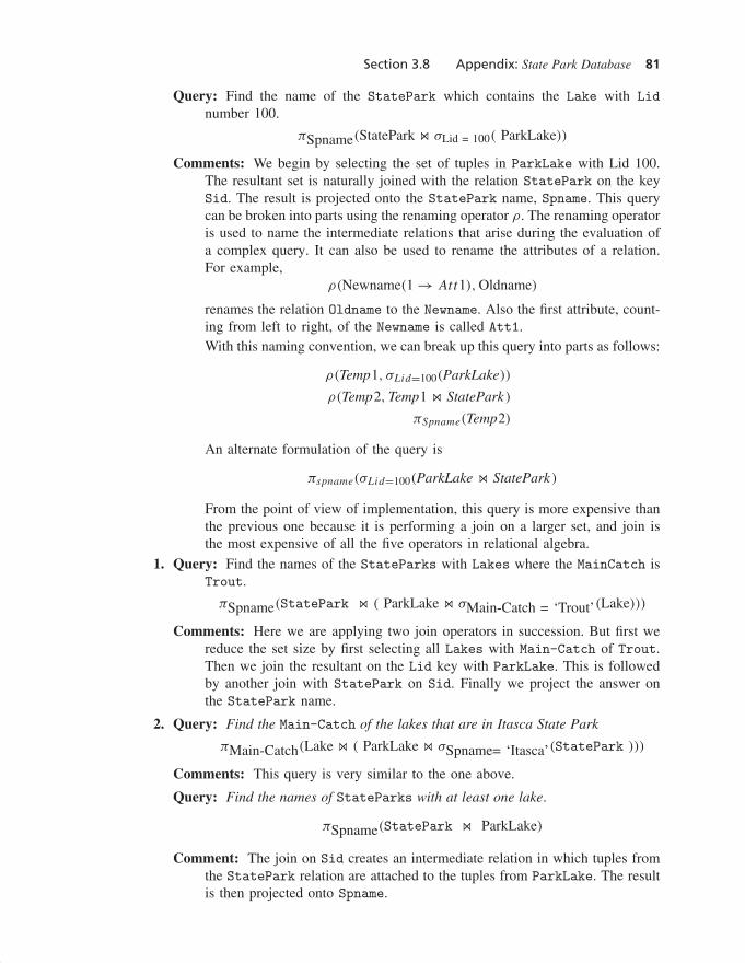
TABLE 3.13: Tables for the StatePark Database

Park Sid Sname Area DistanceS1 Itasca 150.0 52S2 Woodbury 255.0 75S3 Brighton 175.0 300

(a) Park

Lake Lid Lname Depth Main-Catch100 Lino 20.0 Walleye200 Chaska 30.0 Trout300 Sussex 45.0 Walleye400 Todd 28.0 Bass

(b) Lake

ParkLake Lid Sid Fishing-Opener100 S1 05/15200 S1 05/15300 S3 06/01

(c) ParkLake


�

�

�

�

�

�

�

�

Section 3.8 Appendix: State Park Database 81

Query: Find the name of the StatePark which contains the Lake with Lid

number 100.

πSpname(StatePark �� σLid = 100( ParkLake))

Comments: We begin by selecting the set of tuples in ParkLake with Lid 100.The resultant set is naturally joined with the relation StatePark on the keySid. The result is projected onto the StatePark name, Spname. This querycan be broken into parts using the renaming operator ρ. The renaming operatoris used to name the intermediate relations that arise during the evaluation ofa complex query. It can also be used to rename the attributes of a relation.For example,

ρ(Newname(1 → Att1),Oldname)

renames the relation Oldname to the Newname. Also the first attribute, count-ing from left to right, of the Newname is called Att1.With this naming convention, we can break up this query into parts as follows:

ρ(Temp1, σLid=100(ParkLake))

ρ(Temp2, Temp1 �� StatePark)

πSpname(Temp2)

An alternate formulation of the query is

πspname(σLid=100(ParkLake �� StatePark)

From the point of view of implementation, this query is more expensive thanthe previous one because it is performing a join on a larger set, and join isthe most expensive of all the five operators in relational algebra.

1. Query: Find the names of the StateParks with Lakes where the MainCatch isTrout.

πSpname(StatePark �� ( ParkLake �� σMain-Catch = ‘Trout’(Lake)))

Comments: Here we are applying two join operators in succession. But first wereduce the set size by first selecting all Lakes with Main-Catch of Trout.Then we join the resultant on the Lid key with ParkLake. This is followedby another join with StatePark on Sid. Finally we project the answer onthe StatePark name.

2. Query: Find the Main-Catch of the lakes that are in Itasca State Park

πMain-Catch(Lake �� ( ParkLake �� σSpname= ‘Itasca’(StatePark )))

Comments: This query is very similar to the one above.

Query: Find the names of StateParks with at least one lake.

πSpname(StatePark �� ParkLake)

Comment: The join on Sid creates an intermediate relation in which tuples fromthe StatePark relation are attached to the tuples from ParkLake. The resultis then projected onto Spname.


�

�

�

�

�

�

�

�


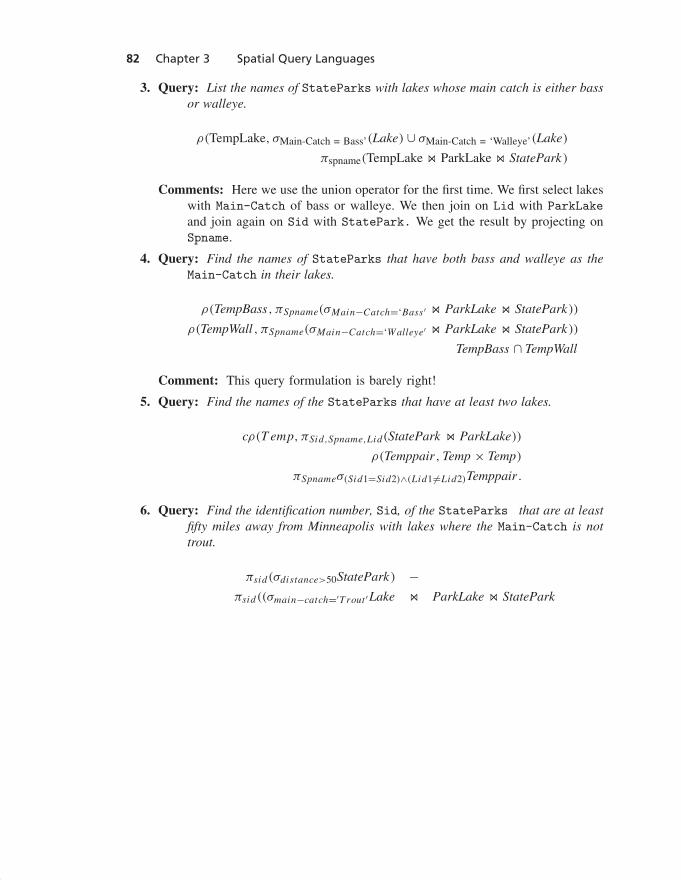
3. Query: List the names of StateParks with lakes whose main catch is either bassor walleye.

ρ(TempLake, σMain-Catch = Bass’(Lake) ∪ σMain-Catch = ‘Walleye’(Lake)

πspname(TempLake �� ParkLake �� StatePark)

Comments: Here we use the union operator for the first time. We first select lakeswith Main-Catch of bass or walleye. We then join on Lid with ParkLake

and join again on Sid with StatePark. We get the result by projecting onSpname.

4. Query: Find the names of StateParks that have both bass and walleye as theMain-Catch in their lakes.

ρ(TempBass, πSpname(σMain−Catch=‘Bass′ �� ParkLake �� StatePark))

ρ(TempWall , πSpname(σMain−Catch=‘Walleye′ �� ParkLake �� StatePark))

TempBass ∩ TempWall

Comment: This query formulation is barely right!

5. Query: Find the names of the StateParks that have at least two lakes.

cρ(T emp, πSid,Spname,Lid(StatePark �� ParkLake))

ρ(Temppair, Temp × Temp)

πSpnameσ(Sid1=Sid2)∧(Lid1�=Lid2)Temppair .

6. Query: Find the identification number, Sid, of the StateParks that are at leastfifty miles away from Minneapolis with lakes where the Main-Catch is nottrout.

πsid(σdistance>50StatePark) −πsid((σmain−catch=′T rout ′Lake �� ParkLake �� StatePark

spatial query languages - wordpress.com · 2008-07-05 · “runall” 2002/5/29 page 52 chapter 3...

Documents